Universidade do MinhoEscola de EngenhariaDepartamento de Informatica

Fabio Esteves Sousa

AuTGen-C: a platform for automatic test datageneration using CBMC

October 2015

Universidade do MinhoEscola de EngenhariaDepartamento de Informatica

Fabio Esteves Sousa

AuTGen-C: a platform for automatic test datageneration using CBMC

Master dissertationMaster Degree in Computing Engineering

Dissertation supervised byMaria Joao Gomes FradeClaudio Belo Lourenco

October 2015

Acknowledgements

I would like to thank everyone who supported me at this stage. Especially to my supervisors,Maria Joao Frade and Claudio Belo Lourenco, for all the effort and time dedicated.

A B S T R AC T

The importance of good test cases is universally recognized and so is the high costs associated to their

manual generation.

Software testing via coverage analysis is the most popular and used technique for software verifi-

cation in industry but remains one of the most expensive tasks in the software development life cycle,

since manual generation is often involved.

Mechanised verification techniques can have a role in the automated test generation, reducing the

costs of the generation process and producing good quality tests. An example of this is the use of

bounded model checkers of software for this purpose, having as flagship the CBMC tool for ANSI-C

code. In Angeletti et al. papers [1, 2] it is described how CBMC was used as an automatic test data

generator for coverage analysis of safety-critical software in an industrial setting. The motivation for

this dissertation was to explore, implement, and extend the ideas presented in those works and to build

an open-source tool for test data generation based on CBMC.

We have designed and implemented the AuTGen-C tool, a platform for the automatic generation of

set of tests for C programs with high level of coverage (always trying to reach 100%), totally based

on the CBMC tool.

A new technique was devised for instrumenting the code based on the introduction of fresh-variables

that allows for a greater control over the process of test generation, and allows us to perform the cov-

erage analysis based on the responses obtained from CBMC. Thereby, we avoid the use of an external

tool to check the level of coverage achieved. Based on this technique, we have developed two dif-

ferent methodologies: the fresh-variable methodology for single location, which generates each test

having as target a specific location of the code; and the fresh-variable methodology for multi-locations,

which generates each test having as target a set of locations in the code. For the application of the later

methodology we previously construct sets of locations that potentially can be reached in a single run

of the program (i.e., that belong to some path). The motivation behind this ideia is to try to achieve

the same coverage level with smaller test sets.

The methodologies implemented in the AuTGen-C tool are for the decision coverage criterion, but

the same approach can be used for different criteria. In this dissertation we also discuss how those

methodologies could be adapted to condition coverage and condition/decision coverage criteria.

The AuTGen-C tool is available and ready to be used. We experimentally evaluated the effective-

ness of the AuTGen-C tool by running it over several case studies including the popular open-source

application grep. These preliminary experiments were very encouraging.

i

R E S U M O

O teste de software baseado na analise de cobertura do codigo e uma tecnica muito utilizada para a

verificacao de software na industria, mas continua a ser um dos processos mais caros do seu desen-

volvimento visto que a geracao de bons casos de teste e por vezes um processo manual.

As tecnicas de verificacao automatica de software podem ter um papel na automatizacao do pro-

cesso de geracao de testes de qualidade, reduzindo muito os custos associados a sua producao. Um ex-

emplo disso e a utilizacao para este fim de software bounded model checkers (de onde se destaca a fer-

ramenta CBMC para verificacao de codigo C). Angeletti et al. descrevem em [1, 2] uma aplicacao com

elevado sucesso do CBMC na geracao automatica de testes com alta taxa de cobertura, no contexto

industrial do sistema europeu de controlo de linhas ferroviarias. A motivacao para esta dissertacao foi

explorar, implementar e extender as ideias apresentadas nesses trabalhos, e construir uma ferramenta

(de codigo aberto) para geracao automatica de testes baseada no CBMC.

No ambito deste projecto desenvolvemos a ferramenta AuTGen-C, uma plataforma para a geracao

automatica de testes, para programas C, com um nıvel muito elevado de cobertura (tentando sempre

atingir 100%), totalmente baseado na ferramenta CBMC. Desenvolvemos uma nova tecnica de in-

strumentar o codigo, com base na introducao de variaveis novas, que nos permite um maior controle

sobre o processo de geracao de testes e nos possibilita fazer a analise de cobertura com base nas re-

spostas obtidas do CBMC, evitando assim a utilizacao de uma ferramenta externa. Com base nesta

tecnica, desenvolvemos duas metodologias diferentes para a geracao de testes: uma metodologia que

se foca num unico local do codigo de cada vez que se gera um teste; e uma outra metodologia que

tem como alvo um conjunto de locais do codigo que sao previamente calculados de forma a que ten-

ham potencial para serem cobertos por um unico teste. A motivacao para esta segunda metodologia e

tentar alcancar um elevado nıvel de cobertura com um conjunto mais reduzido de testes. Discutem-se

tambem como estas metodologias podem ser aplicadas para outros criterios de cobertura. Por fim

e feita uma avaliacao experimental da ferramenta AuTGen-C aplicando-a a varios casos de estudo

incluindo a popular aplicacao grep. Os resultados que obtivemos foram bastante encorajadores.

ii

C O N T E N T S

Contents iii

1 I N T RO D U C T I O N 1

1.1 Motivation 1

1.2 Contributions 3

1.3 Document Structure 4

2 B AC K G RO U N D 5

2.1 An Overview in Software Testing 5

2.1.1 Software Testing Over Time 5

2.1.2 Levels of Software Testing 6

2.2 Code Coverage 7

2.2.1 Statement Coverage 8

2.2.2 Decision Coverage or Branch Coverage 9

2.2.3 Condition Coverage 10

2.2.4 Decision/Condition coverage 10

2.2.5 Modified Condition / Decision Coverage 11

2.2.6 Multiple Condition Coverage 12

3 T E S T DATA G E N E R AT I O N U S I N G B O U N D E D M O D E L C H E C K I N G 13

3.1 Software Bounded Model Checking 14

3.1.1 Inserting Specific Properties 14

3.1.2 The Bounded Model Checking Technique 15

3.1.3 Checking for Property Violation 18

3.2 Test Data Generation using Bounded Model Checking 19

3.2.1 Test Data Generation 19

3.2.2 Improving Test Data Generation 24

4 O U R A P P RO AC H F O R T E S T DATA G E N E R AT I O N U S I N G C B M C 27

4.1 Signalling Locations 28

4.1.1 The Token Technique 28

4.1.2 The Fresh-Variable Technique 29

4.2 Methodologies 30

4.2.1 The Token Methodology 31

4.2.2 The Fresh-Variable Methodology for Single Location 32

4.2.3 The Fresh-Variable Methodology for Multi-Locations 33

4.3 Extending to Other Code Coverage Criteria 37

iii

Contents

4.3.1 Condition Coverage 37

4.3.2 Condition/Decision Coverage 40

5 AuTGen-C T O O L 42

5.1 Architecture and Implementation Choices 42

5.1.1 Tools, Language and Libraries 42

5.1.2 Architecture and Source Code Structure 43

5.2 Pre-Instrumentation 45

5.3 Instrumentation Process for Decision Coverage 47

5.4 Set of Locations Sets Generation 50

5.5 Test Generation and Test Vector Extraction Processes 52

5.5.1 CBMC Interaction and Test Construction 52

5.5.2 CBMC Limitations 54

5.6 The Unit Used 54

5.7 Tool Guide 55

6 E VA L UAT I O N A N D C O N C L U S I O N S 57

6.1 Tool Evaluation 57

6.2 Global Analysis 62

6.3 Conclusion 63

6.4 Future Work 64

iv

L I S T O F F I G U R E S

Figure 1 Foo function 8

Figure 2 Control flow graph of the function in Figure 1 8

Figure 3 Code example with no decision 10

Figure 4 Code example with no decision 10

Figure 5 Conjunctions 11

Figure 6 Disjunctions 11

Figure 7 Code example with assert statement with if statement 14

Figure 8 Code example with assumption statement with if statement 15

Figure 9 Normalization to a subset of instructions 15

Figure 10 An automatic instrumentation. Array bounds for i and max. Overflow in

variable i. 16

Figure 11 In the left, the code to be unwind. In the right, the code with unwind assump-

tion. In the center, the code with unwind assertion. The loops are unwound

with a bound of 2. 16

Figure 12 An unwinding assertion transformation from Figure 10 17

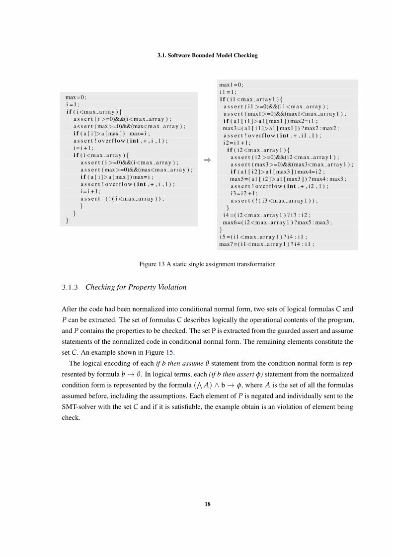
Figure 13 A static single assignment transformation 18

Figure 14 An normalized code in conditional normal form 19

Figure 15 Extracted formulas from normalized code in conditional normal form 19

Figure 16 Test coverage generation process. 20

Figure 17 Provide non-deterministic input to a function called fut 21

Figure 18 Code exemple of #ifdef macro 21

Figure 19 A fragment of a trace form the CBMC command output. The example target

ASSERT 1 form the function in Figure 20 22

Figure 20 Left side is the function before instrumentation step with comments in the

location needed to obtain test (for the reader best understanding). Right side

the function after pass the instrumentation step. 23

Figure 21 Test coverage generation process. 24

Figure 22 Peace of code to be use as a example 25

Figure 23 Transformed code from Figure 22 26

Figure 24 Example of a #ifdef macro 28

Figure 25 A code fragment of Maxmin6varKO function with variable technique 30

Figure 26 Piece of code where Maxmin6varKO is called with necessary annotation to

generate a test 30

v

List of Figures

Figure 27 Test case generation following the token methodology 31

Figure 28 The algorithm relative to the test generation step for the fresh-variable method-

ology for a single location 33

Figure 29 The algorithm relative to the test generation step for the fresh-variable method-

ology for a multi-locations 35

Figure 30 Bubble sort function 36

Figure 31 An sketch of idea to check condition in a decision 38

Figure 32 The outcome form the token technique applied to a if statement for condition

coverage. 38

Figure 33 The outcome form the fresh-variable technique applied to an if command for

condition coverage. 39

Figure 34 The outcome form the fresh-variable technique applied to an if command for

condition/decision coverage. 40

Figure 35 The outcome form the token technique applied to a if command for condi-

tion/decision coverage 41

Figure 36 Tool architecture 43

Figure 37 Structure of the tool filesystem 45

Figure 38 Part of program emphasizing non-deterministic initialization 46

Figure 39 Part of program emphasizing an alternative initialization method 46

Figure 40 Part of program emphasizing an alternative initialization method 46

Figure 41 Part of program emphasizing an alternative initialization method 47

Figure 42 Annotation type definition 48

Figure 43 The auxiliary variable type definition 49

Figure 44 Annotations pretty print 49

Figure 45 Statements pretty print 50

Figure 46 The commands in the reduced abstract syntax tree 51

Figure 47 The trap function instrumented using the fresh-variable technique 51

Figure 48 XML assignment 53

Figure 49 Test vectors file 54

Figure 50 The function dependencies 55

vi

L I S T O F TA B L E S

Table 1 The bubble sort evaluation results 58

Table 2 The maxmin6var evaluation results 59

Table 3 The cars evaluation results 60

Table 4 The grep evaluation results 61

vii

1

I N T RO D U C T I O N

1.1 MOTIVATION

Nowadays it is increasingly important to ensure quality in the produced software. Defects in software

result in high costs and operational inefficiencies. Software testing is the technique embraced by the

software industry to certify and ensure quality in software products. Fifty percent of the development

time and between thirty four up to fifty percent of the total costs are related to software testing. These

percentages have not changed along the years [17], which indicate us that there is some progress that

can be made.

Failures due to software defects may have serious consequences. An emblematic case with serious

consequences was the multiple failures in the automated baggage system due to software errors at

Denver International Airport [12]. The software errors in the system had initially delayed the airport

inauguration by 16 months and after eleven years of unreliable service, the automated baggage handler

had to be pluged-out and converted into a traditional service using manual carts and tugs with human

drivers.

What happened at Denver International Airport is not an isolated case. A report presented by Tassey

[24] in 2002 indicates that national annual costs due to inadequate software testing was estimated to

range from $22.2 to $59.5 billion only in the United States of America. Among the contributing fac-

tors are under-budget test resources, inadequate methods, tight schedules, poor requirements design,

low level testing, poor test management, unskilled/untrained testers and inadequate use of automated

testing tools.

High costs in software production normally comes from defects that are discovered in later stages

of software development. Several studies [19, 20, 22] reported the costs associated to the repair of

software escalates enormously from phase to phase. Reasons that can justify such behaviours are

related to defects that propagate through the software life cycle resulting in an expensive and time-

consuming redesign which by itself creates new defects.

Certification and quality is crucial when the topic is critical software. A software system is consid-

ered critical if it may cause severe injury to human lives or occupational illness, and/or major damage

to facilities, systems, or hardware [21]. A common regulatory feature of all safety-critical software

standards is that software must demonstrate, through rigorous testing and documentation that it is well

1

1.1. Motivation

designed and operates safely. Testing of safety-critical software includes code coverage and analysis

to insure that all program instructions are tested. This requirement substantially increases the costs

associated to testing task since it often involves the manual generation of tests.

Testing has been the primary way that software is checked for correctness. However testing requires

substantial resources and can rarely check all possible execution scenarios. Tests are usually created

based on the most likely usage of the software or on intuition where a bug may lie. This often results

in undetected errors. Another way to guarantee the correctness of software is by using program veri-

fication techniques. There are different approaches to program verification. The deductive approach

is based on the use of a program logic and the design-by-contract principle, and it allows for express-

ing properties using a rich specification language. However deductive verification lacks automation -

tools for deductive verification requires a lot of human intervention and working with them is a very

specialised job and may require a lot of effort.

Another approach to program verification is based on model checking and abstraction techniques.

Model checking of software, which typically allows only for simpler properties, expressed as asser-

tions in the code, but is fully automated. The fundamental idea is to create a model from the source

program, and then, given a property, to check if it holds in that model. However, such an approach

has a main downside: state space explosion. Existential abstraction [8] and bounded model check-

ing [5] are two approaches that can be used to overcome this limitation. The former is a conservative

technique: it introduces false positives (false warnings), sacrificing completeness, while the latter tech-

nique only checks execution paths with size up to a fixed (user-provided) bound, sacrificing soundness.

The false positives introduced by abstraction techniques must be manually filtered from the real bugs

and can become an overwhelming task. The soundness of the bounded model checking technique can

be regained by conservatively introducing special “unwinding” assertions to check that longer execu-

tion paths cannot occur during execution of the program, but the general idea is that only a partial

exploration of the state space is performed.

Despite the enormous improvements in verification tools in the last decade, their use in the verifica-

tion of software with some complexity may have high costs. This fact has made verification accessible

to only the most safe-critical software and not to most commercial software.

The importance of good test cases is universally recognized and so is the high cost of generating

them by hand. Mechanized verification techniques can have a role in the automated generation of

tests. In the recent years, testing and verification have come close together.

An example of this is the use of bounded model checkers of software, having as flagship the CBMC

tool [7] for ANSI-C code. The key idea of bounded model checking of software is to encode bounded

behaviours of the program that enjoy some given property as a logical formula whose models, if any,

describe execution paths leading to a violation of the property. The properties to be established are

assertions on the program state, included in the program through the use of assert statements. For

every execution of the program, whenever a statement assert φ is met, the assertion φ must be

satisfied by the current state, otherwise we say that the state violates the assertion φ. The verification

2

1.2. Contributions

technique assumes that a satisfiability-based tool is used to find models corresponding to property

violations.

This technique can be very helpful in finding inputs that make the program execute some improvable

path where a bug may be hidden. These kind of bugs are rarely discovered by pure directed testing

algorithms. Rather than demonstrating program correctness, the focus of this technique is finding bugs

in real-world programs. The ability to express properties as assertions, and to return an assignment to

input variables falsifying the property make bounded model checking of software particularly tailored

to automatic test data generation.

In Angeletti et al. [2] it is described how CBMC has been used for coverage analysis of safety-

critical software in an industrial setting. In particular, they experimented CBMC on a subset of the

modules of the European Train Control System (ETCS) of the European Rail Traffic Management

System (ERTMS) source code, an industrial system for the control of the traffic railway. The method-

ology they proposed was applied to the ERTMS/ETCS, with thousands of lines, obtaining a set of

tests that covers 100% of the code coverage, requested by the CENELEC EN50128 guidelines for

software development of safety critical systems.

In another paper [1] Angeletti et al. present a new methodology for the automatic test data gen-

eration based on the use of CBMC, with the aim of improving the quality of the test set generated,

in the sense of avoiding the production of redundant tests i.e. the test generation of tests that do not

contribute to reach the property of 100% of code coverage. Indeed, these redundant tests are useless

from the perspective of the coverage, and they are not easy to detect and to remove a posteriori, and,

if maintained, imply additional costs during the verification process.

The tools described in the Angeletti et al. papers are not available for public usage. The motivation

for this dissertation was to explore, implement, and extend the ideas presented in those papers and to

build an open-source tool for test data generation based on CBMC.

1.2 CONTRIBUTIONS

The main contribution of this dissertation is the design and implementation of the AuTGen-C tool,

a platform for the automated test data generation for C programs with a very high level of coverage

(100% if possible), totally based in the CBMC tool. The AuTGen-C tool is open source, and can be

obtained in https://bitbucket.org/Esteves/autgen-c.

We began by implementing the technique described in [2] but without using an external tool for

the coverage analysis step (as it is done in the original work), because we did not find a freeware tool

suiting our purpose. Without having the tools to do the coverage analysis, the only way to guarantee

that we reach the highest level of code coverage with the generated tests is by having a high degree of

redundancy - a test is generated for each location.

To overcome this difficulty we invented a new technique based on the introduction of fresh variables

to signalise the various points in the code required to be reached by the code coverage criterion. This

3

1.3. Document Structure

technique, in addition to allow greater control over the process of test generation, allows us to perform

the coverage analysis based on the responses obtained from CBMC, thereby avoiding the use of an

external analysis tool.

Based on this technique, we have developed two different methodologies: the fresh-variable method-

ology for single location which generates tests having as target a specific location of the code, and the

fresh-variable methodology for multi-locations which generates tests having as target a set of locations

in the code. For the application of the later methodology we previously construct sets of locations that

potentially can be reached in a single run of the program. The motivation behind this idea is to try to

achieve the same coverage level with a smaller set of tests.

The methodologies implemented in the AuTGen-C tool are for the decision coverage criterion, but

the same approach can be used for other coverage criteria. In this dissertation we also discuss how

those methodologies could be adapted to condition coverage and condition/decision coverage criteria.

1.3 DOCUMENT STRUCTURE

The rest of the dissertation is organized as follows. Chapter 2 gives an overview of software testing

and describes precisely the different criteria of code coverage.

Chapter 3 is devoted to bounded model checking of software and its use in automatic test data

generation. The first part of the chapter describes the necessary transformations to perform bounded

model checking of software, detailing all the steps involved in the extraction of a logical model from

a program. In the second part we descrive the ideas presented in [1, 2] for the automatic test data

generation based on the use of CBMC.

Chapter 4 is devoted to the description of the techniques and methodologies developed by us and

implemented in the AuTGen-C tool. We describe two different techniques for signalling locations in

the code: the first one following the ideias described in Chapter 3 and then a new technique that we

designed to overcome the problems found in the first. Based on those techniques, we then explain the

three methodologies developed for decision coverage. Finally, we discuss how the condition coverage

and condition/decision coverage criteria could also be achieved.

Chapter 5 focuses on the implementation of the AuTGen-C tool. We present the architecture of

the tool and its implementation details. We discuss the design choices, how we have implemented

the key topics described in the previous chapters, the challenges founded and the solutions for those

challenges. We end the chapter with a mini-tutorial about the tool usage.

Chapter 6 is devoted to the evaluation of the AuTGen-C tool, and to present some conclusions

about the work developed. We perform an empirical study comparing the different methodologies im-

plemented in the tool using several case studies. We analyse the results obtained and the performance

of the tool, and then we conclude and point out some directions for future work.

4

2

BAC K G RO U N D

In this chapter we give an overview of software testing and some basic concepts that we use throughout

this document. We focus on description of the different code coverage criteria and its advantages and

disadvantages.

2.1 AN OVERVIEW IN SOFTWARE TESTING

Software testing scope and goals changed over the time. Initially it started as a debugging method to

reveal errors and evolved into guarantee the quality in the software being test. Nowadays, software

testing is a vast area containing a large number of techniques and several criteria to categorize them.

2.1.1 Software Testing Over Time

Throughout time software testing was looked upon different perspectives. Gelperin and Hetzel in

[9] classified and delimited different periods of software testing by scope and goals over time. Until

1956 there was no clear difference between testing and debugging: it was the debug-oriented period.

1957-1978 is classified as the demonstration-oriented period, where “make sure the program runs” and

“make sure the program solves the problem” defined the software testing process. 1979-1982 is named

destruction-oriented period, where testing was understood as “the process of executing a program with

the intent of finding errors”. 1983-1987 is called the evaluation-oriented period, characterised by the

introduction of methodologies (such as analysis, reviews and test activities) during all the software

development cycle to provide product evaluation. In 1988 we entered in the prevention-oriented

period, where the testing process is more professional and aims not only the detection and prevention

of faults but also that software satisfies its requirements. In [9] the authors highlight the creation and

use of methodologies that define the software testing tasks to take place parallel to the development

of the code.

Gelperin and Hetzel was published [9] in 1988 and it is our opinion that the last period defined

by them as already passed. Nowadays, software testing is seen as “The process of revealing defects

in the code with the ultimate goal of establishing that the software has attained a specified degree of

quality”[11].

5

2.1. An Overview in Software Testing

2.1.2 Levels of Software Testing

Nowadays, software testing is seen as part of software development and it is divided in different levels.

The most common levels are unit, integration, system and acceptance. Each level has its own purpose

and they are performed in sequence. Automated test data generators can be generate from unit level

to system level, but they normally are more used in the unit level for scalability reasons.

Unit Testing

Unit testing is a level of software testing process where individual units are tested. The purpose of

unit tests is to validate that each unit performs as designed. In other words, if they are fit for use.

Even though a unit is considered to be the smallest testable part, in the test generation community,

when it comes to define this part there is not a common opinion. For some it could be a simple function

but for others it could be a set of functions or even the whole module.

Integration Testing

Integration testing is a level of software testing process with the objective to identifies problems that

occur when units are combined. In other words, units that had already been tested are now combined

as one component and then is tested the interface between them. The integration testing proceeds the

unit testing.

There is two different approach when applying the integration test. The top-down and the bottom-

up. Also exists some references to a third one, the umbrella approach.

- Top-down: “The top-down approach to integration testing requires the highest-level modules

be test and integrated first. This allows high-level logic and data flow to be tested early in the

process and it tends to minimize the need for drivers. However, the need for stubs complicates

test management and low-level utilities are tested relatively late in the development cycle. An-

other disadvantage of top-down integration testing is its poor support for early release of limited

functionality.”[16]

- Bottom-up: “The bottom-up approach requires the lowest-level units be tested and integrated

first. These units are frequently referred to as utility modules. By using this approach, utility

modules are tested early in the development process and the need for stubs is minimized. The

downside, however, is that the need for drivers complicates test management and high-level

logic and data flow are tested late. Like the top-down approach, the bottom-up approach also

provides poor support for early release of limited functionality.”[16]

- Umbrella: “The umbrella approach requires testing along functional data and control-flow paths.

First, the inputs for functions are integrated in the bottom-up pattern discussed above. The out-

puts for each function are then integrated in the top-down manner. The primary advantage of

6

2.2. Code Coverage

this approach is the degree of support for early release of limited functionality. It also helps

minimize the need for stubs and drivers. The potential weaknesses of this approach are signif-

icant, however, in that it can be less systematic than the other two approaches, leading to the

need for more regression testing.”[16]

System Testing

System testing is the level of software testing process where the behaviour of whole system/product

is tested, to verify the system meets the specification and its purpose. It is is carried out by specialists

testers or independent testers and should investigate both functional and non-functional requirements

of the testing.

Acceptance Testing

Acceptance Testing is a level of the software testing process where a system has met the requirement

specifications, and now will be the tested for acceptability. The main purpose of this test is to evaluate

the system’s compliance with the business requirements and verify if it has met the required criteria

for delivery to end users. This should be fulfilled by elements that are not the coders of the software.

The acceptance testing can be divided in two major steps normally referenced as alpha testing and

beta testing.

- Alpha Testing: The Alpha testing is when the acceptability are realized by the programmer with

direct knowledge of the code but not involve in their development. The primary objective in

this phase is the validation tests realized by the coder team.

- Beta Testing: The Beta testing is when the acceptability are realized by the customer side, It

involves testing by a external group formed by customers or possible future users who use the

system at their own locations and provide feedback. This append before the system is released

to customers.

2.2 CODE COVERAGE

Code coverage is a measure for describing the degree to which the source code of a program is tested

by a set suite. It is a quality assurance metric which determines how exhaustively a set of tests

exercises a given program.

The coverage criteria establish the rules a test suite needs to satisfy. The percentage of code ex-

ercised by a test suite is measured according to such criteria. There are many different criteria such

as: statement coverage, decision coverage, condition coverage, multiple condition coverage, condi-

tion/decision coverage and modified condition/decision coverage, among others. Next we will give a

description of such code coverage criteria.

7

2.2. Code Coverage

void foo(int A,int B,int X) {if(A>1 && B==0) {X=X/A;

}if(A==2 || X>1) {X=X+1;

}}

Figure 1 Foo function

Figure 2 Control flow graph of the function in Figure 1

2.2.1 Statement Coverage

Statement Coverage criterion states that one must write enough tests so that every state-

ment in the program must be executed at least once.

Consider the function in Figure 1 and its control flow graph in Figure 2. If we want to generate

the necessary set of tests to achieve statement coverage for the code presented in Figure 1, the test

vectorA = 2, B = 0, X = 3 is the only test necessary to achieve this criterion. The execution of this

test passes throughout all the statements and follows the path ace in graph in Figure 2.

Considerations when applying this criterion

This criterion is consider rather weak and generally useless[17]. Considering the previous example,

the path abd where X is kept unchanged will never be executed. The reason why this happens is

because there exist no statement throughout the path abd, so if there is any error it would go unnoticed.

8

2.2. Code Coverage

2.2.2 Decision Coverage or Branch Coverage

Decision Coverage criterion states that every decision in the program must take all possi-

ble outcomes at least once, and every entry and exit point in the program has been invoked

at least once.

To achieve full decision coverage for the code in Figure 1, it is enough to generate a set of tests for

the paths (ace, abd) or for the paths (acd, abe) from Figure 2. In both cases the paths pass throughout

all decisions in the program obtaining true and false outcome.

Considerations when applying this criterion

Although decision coverage criterion is considered a stronger criterion than statement coverage crite-

rion, it is viewed as rather weak. It exists a probability of 50 percent that the path where variable X is

unchanged, the abd path, will not be considered.

Consideration when defined this criterion

There is no clear consensus in the testing community when it comes to define decision or branch

coverage. In the following paragraphs we present different definitions for decision or branch coverage.

The authors of [17] initially described this coverage criterion as “Must be written enough test cases

that each decision has a true and a false outcome at least once”, however, the authors rewrites the

definition after comparing it with the statement coverage. The authors affirms that decision coverage

is superior to statement coverage and, therefore, the decision coverage must also contemplate the cases

coverage by the statement coverage criterion. The new definition provided by the authors to decision

coverage is “Decision coverage requires that each decision have a true and a false outcome, and that

each statement be executed at least once.” or “An alternative and easier way of expressing it is each

decision has a true and a false outcome, and that each point of entry be invoked at least once.”

Other definition for the decision coverage is presented by Kelly J. et al. [15] which defines decision

coverage criterion as “Every decision in the program has taken all possible outcomes at least once and

every point of entry and exit in the program has been invoked at least once.”.

Also Naik and Tripathy [18] defines differently the decision coverage criterion. Citing the author

(that uses the term branch coverage instead of decision coverage), derision coverage criterion is “Se-

lecting program paths in such a manner that certain branches (i.e., outgoing edges of nodes) of a

control flow graph are covered by the execution of those paths. Complete branch coverage means

selecting some paths such that their execution causes all the branches to be covered”.

If we had only defined the decision coverage as “Every decision in the program has taken all pos-

sible outcomes at least once”, it would exist examples of code where no tests would produced. For

instance, the code shown in Figure 3 does not have any decision, therefore, no tests would be gener-

ated. Requiring also that every entry point in the program be invoke at least once solves this problem.

9

2.2. Code Coverage

void foo(int A,int B,int X) {A=A+1;B=A;

}

Figure 3 Code example with no decision

Another solution would be require that every exit point in the program be invoke at least once. More-

over, it would also allows to identify some cases of dead code. For instance, in the program of Figure 4,

the code after the return A statement would be identified as dead code.

int foo(int A,int B,int X) {...return A;A=A+1;B=A;return B;

}

Figure 4 Code example with no decision

The C language do not allows functions with multi-entry points. Thereby, the criterion “Every

decision in the program has taken all possible outcomes at least once and every exit point in the

program has been invoked at least once” is enough to achieve the same paths as the criterion “Every

decision in the program has taken all possible outcomes at least once and every point of entry and exit

in the program has been invoked at least once”.

2.2.3 Condition Coverage

The condition coverage criterion states that each condition in a decision must take all

possible outcomes at least once and every entry and exit in the program must be least

once.

Considering the code listed in Figure 1 the minimum number of tests needed to achieve this code

coverage criterion is only two. Using only this two tests {(A = 2,B = 0,X = 2),(A = 1,B = 1,X = 1)}

is possible to reach 100% of condition coverage. Note that in the present example, for both tests, the

first decision is always true and the second decision is always false.

2.2.4 Decision/Condition coverage

The decision/condition coverage criterion requires that each condition in a decision takes

on all possible outcomes at least once, each decision takes on all possible outcomes at

least once, and each entry point and exit point is invoked at least once.

10

2.2. Code Coverage

To completely achieve decision/condition coverage for the code in Figure 1 the set of tests { (A =

2, B = 0, X = 4), (A = −1, B = −1, X = −1) } is enough. All condition are evaluated to true and to false,

and the decisions are also evaluated to true and to false.

This criterion is a merge of decision coverage and condition coverage. The objective is to overcome

some limitations found in both criteria.

2.2.5 Modified Condition / Decision Coverage

The modified condition/decision coverage criterion states that every entry and exit point in

the program has to be invoked at least once, every condition in a decision in the program

has to take take all possible outcomes at least once, and each condition in a decision has

to be shown to independently affect that decision’s outcome.

The criterion improves the condition/decision coverage by requiring that each condition indepen-

dently affect the outcome of the decision. The application of this criteria to the code in Figure 1 could

be achieved with the following tests{(A = 2, B = 0, X = 2), (A = 1, B = 1, X = 1), (A = 0, B = 0, X = 2)}.

Considerations when applying this criterion

The generation of tests according to modified condition/decision coverage is more complex compara-

tively to condition/decision coverage. In the following lines we describe in detail how to generate the

necessary tests to this criterion.

if (A && B && C) {...

}

Figure 5 Conjunctions

if (A || B || C) {...

}

Figure 6 Disjunctions

The decisions formed by an and operator or by an or operator are generated differently. A condition

is shown to independently affect a decision outcome by varying just its value while keeping fixed the

value of all the others conditions.

Following the nature of and operator, to ensure a condition is independently affecting the decisions

outcome, the condition must be set to false and all the remaining conditions set to true. So the set

of tests necessary to achieve the modified condition in Figure 5 is the set of tests {(A = False, B =

True, C = True), (A = True, B = False, C = True), (A = True, B = True, C = False)}. But to achieve the

modify condition/decision coverage it is also needed to add the test (A = True, B = True, C = True) to

obtain all possible decision outcomes.

Relative to the or operator, to ensure a condition is independently affecting the decisions outcome,

the condition must be set to true and all the remaining conditions set to false. So the set of tests

11

2.2. Code Coverage

necessary to achieve the modified condition in the code in Figure 6 is the set {(A = True, B = False, C =

False), (A = False, B = True, C = False), (A = False, B = False, C = True)}. But to achieve the modify

condition/decision coverage it is also needed to add the test (A = False, B = False, C = False) to obtain

all possible decision outcomes.

2.2.6 Multiple Condition Coverage

The multiple condition coverage criterion states one must write a sufficient number of

test cases to invoke all possible combinations of condition outcomes in each decision, and

all points of entry to the program, at least once.

In other words, for a decision with n inputs the multiple condition coverage requires 2n tests.

12

3

T E S T DATA G E N E R AT I O N U S I N G B O U N D E D M O D E L C H E C K I N G

Model checking is a verification technique that explores all possible system states a in brute-force

manner. In this way, it can be shown that a given model satisfies certain properties [3]. When ap-

plied to software, model checking can be defined as an analysis algorithm that proves properties over

program executions [13]. One of the disadvantages of this technique is the exponential growth in the

number of states. Such is due to several factors, such as the number of variables or their representa-

tion size, which makes models too large for the current available resources. In an attempt to avoid

the growth in the number of states a new technique called bounded model checking was introduced in

1999.

Bounded model checking was introduced in Biere et al. [5] for LTL (Linear temporal logic) through

propositional decision procedures. Linear temporal logic is modal temporal logic widely used at

the time to prove properties about programs since it allows to write formulas about the future of

paths. Later this technique was extended to software. First developments in software bounded model

checking initiated around the year 2004 and published in Clarke et al. [6, 7]. Clarke et al. presented

in [7] the first bounded model checker targeting exclusively ANSI-C programs where properties to be

verified were established through assertions and assumptions on the program as special statements.

In a simple way, bounded model checking is the same as model checking but the model being

checked is bounded. In software bounded model checking, the model is the software and the bound is

established by unwinding the loops a finite number of times. The bounded model is then transformed

into propositional formulas which are used to prove the validity of the properties that we want to

prove. The correctness obtained when applying this technique is ”partial” in the sense that the model

being verified is not the original one, but only a part of it. This technique only checks executions

with length up to a fixed (user-provided) bound, sacrificing soundness. However ”total” correctness is

possible to achieve if we considered a bound that captures all possible execution behaviours. This can

be consider as a disadvantage due to the general unsoundness of the approach, but on the other hand

can be consider a advantage in finding counterexamples for the properties we want to check. For this

reasons bounded model checking is often used as a bug finder.

Bounded model checking of software has also been applied in the field of automated test generation.

In [2], Angeletti et al. reported a methodology to automatically generate coverage tests to ANSI-C

13

3.1. Software Bounded Model Checking

programs with high degree of coverage. In other paper [1], the same authors present a different

strategy to automatic generate tests and overcome some issues from the previous technique.

In the following sections is discuss in greater detail the bounded model checking of software tech-

nique and its use in the field of automated test generation.

3.1 SOFTWARE BOUNDED MODEL CHECKING

The bounded model checking technique as been largely used in detecting underflow and overflow,

pointer safety, memory leaks, array bounds among others. This section is dedicated to explain the

work-flow of software bounded model checking. In the following subsections we explain how users

can insert their own properties, what should be expected from bounded model checking and how

properties are verified. All the following subsections are based on [3, 5, 6, 7].

3.1.1 Inserting Specific Properties

Bounded model checking tools are fully automatic. They provide safe properties automatically, but

users may annotate the code with properties they want to check. Manual annotations of properties

normally are used for for debugging purposes or to check functional properties. In this dissertation

we will use specific properties to obtain specific counterexamples which are then used as test to reach a

certain coverage criteria. This specifications are normally introduced through statements in the source

code, that are ignored by the compiler.

The standard annotations in bounded model checking of software are assert and assume.

i f ( A | | B ) {a s s e r t (A== t r u e ) ;. . .

}

Figure 7 Code example with assert statement with if statement

The properties we want to verify and expect to always be true are included through the use of assert

statements. For every execution of the program, whenever a statement assertp is met, the property pmust be satisfied by the current state, otherwise we say that the p was violated. When a violation is

found a counterexample is returned to the user. Generally when a bounded model checker finds an

assertion violation, it immediately returns the counterexample and ignores forward assertions. Such

action derives from the nature of SAT solvers. An example of the use of this mechanism is Figure 7

where it is checked if the condition A is always true using the property “A == true”.

The annotation assume p, where p is a property, is used when the user wants to impose that only

the executions satisfying p, at that location, are considered during the verification. In other words,

whenever an assume p is annotated in the code, one wants to restrict the model being verified.

14

3.1. Software Bounded Model Checking

assume (A | |B == t r u e ) ;i f ( A | | B ) {

. . .}

Figure 8 Code example with assumption statement with if statement

An example in the use of this mechanism is Figure 8, where the model was restricted to traces

passing through the true branch of the if condition, at that point, by using “A||B == true” property.

Is import to note that assumptions affect the evaluation of the assertions that occurs after them,

in the sense that an assertion is implied by all previous assumptions. That can lead to a model so

restricted that there are not any trace to be test and every assert will be vacuously true.

3.1.2 The Bounded Model Checking Technique

The Bounded Model Checking technique is divided into several steps. Their main goal is to transform

a program into logical propositions to be checked by a SAT solver.

First, it is applied a process of simplification and transformation of the original program. That

includes the elimination of directives(#de f ine, #include, #i f de f ine, etc..) and side-effects( i++,- -i,

etc...) but also, if intended, the normalization of the program into a subset of the target programming

language. An example of transformation process is show in Figure 9.

f o r ( i =0 ; i <= max ;i ++) {

x=5+(++ j ) ;. . .

}

⇒

i =0 ;whi le ( i <= max ) {

j = j +1 ;x=5+ j ;. . .i = i +1 ;

}

Figure 9 Normalization to a subset of instructions

Secondly, an automatic instrumentation process might be applied to the code. This step is op-

tional. The user may want to check only its own properties. The properties automatically inserted are

normally related to safely violations, such as overflow/underflow, array out of bounds, null pointers,

dereferences, divisions by zero, among others. An example of automatic instrumentation is repre-

sented in Figure 10, where safety properties, related to array out bounds, are introduced in order to

check if the values of i and max always lie in the array bounds. Also safety properties related to over-

flow are inserted to check if the operation i + 1 does not cause an overflow. The predicate !over f lowis used because the encoding of this property might be different depending on the variable type, the

minimum and maximum values are different, and the back-end solver.

15

3.1. Software Bounded Model Checking

max =0;i =1 ;whi le ( i<m a x a r r a y ) {

i f ( a [ i ]>a [ max ] ) max= i ;i = i +1 ;}

⇒

max =0;i =1 ;whi le ( i<m a x a r r a y ) {

a s s e r t ( i >=0 && ( i<m a x a r r a y ) ;a s s e r t ( max>=0 && ( max<m a x a r r a y ) ;i f ( a [ i ]>a [ max ] ) max= i ;a s s e r t ( ! o v e r f l o w ( i n t , + , i , 1 ) ;i = i +1 ;

}

Figure 10 An automatic instrumentation.Array bounds for i and max. Overflow in variable i.

The next step is crucial. Then the programming is unwound a k number of times. The unwind-

ing number k might be inferred automatically, when possible, or else, specified by the user. Loop

constructs, function calls and backwards goto statements are the elements that are unwound.

Loop constructs can be expressed as while statements so all loop constructs are transformed into

while statements, if not already a while statement, and unwound by duplicating the loop body k times.

See Figure 11.

whi le ( b ) {l o o p b o d y ;

}

i f ( b ) {l o o p b o d y ;i f ( b ) {

l o o p b o d y ;a s s e r t ( ! b ) ;

}}

i f ( b ) {l o o p b o d y ;i f ( b ) {

l o o p b o d y ;assume ( b ) ;}

}

Figure 11 In the left, the code to be unwind. In the right, the code with unwind assumption.In the center, the code with unwind assertion.

The loops are unwound with a bound of 2.

Each copy is guarded using an if statement that uses the same condition as the loop statement. Such

is for the case that the loop requires less than k iterations. After the last copy, an annotation with the

negation of the loop condition is added. According to the annotation used, assertion or assumption, is

called unwinding assertion or unwinding assumption. The unwinding assertion is used to know if kbound is actually large enough for any possible execution. If it is not large enough the loop assertion

will fail. An alternative to the unwinding assertion is the use of unwinding assumption. When the

unwinding assumption is used, then every path that requires more then k iterations will not be taken

into account. An example of unwinding a loop twice is shown in Figure 12 and in this case was used

an unwinding assertion.

Backwards goto statements are unwound in a manner similar to while loops. Function calls state-

ments are replaced by the function body, variables are renamed to avoid conflicts between variables,

16

3.1. Software Bounded Model Checking

max =0;i =1 ;whi le ( i<m a x a r r a y ) {

a s s e r t ( i >=0 && ( i<m a x a r r a y ) ;a s s e r t ( max>=0 && ( max<

m a x a r r a y ) ;i f ( a [ i ]>a [ max ] ) max= i ;a s s e r t ( ! o v e r f l o w ( i n t , + , i , 1 ) ;i = i +1 ;

}

⇒

max =0;i =1 ;i f ( i<m a x a r r a y ) {

a s s e r t ( i >=0)&&(i<m a x a r r a y ) ;a s s e r t ( max>=0)&&(max<m a x a r r a y ) ;i f ( a [ i ]>a [ max ] ) max= i ;a s s e r t ! o v e r f l o w ( i n t , + , i , 1 ) ;i = i +1 ;i f ( i<m a x a r r a y ) {

a s s e r t ( i >=0)&&(i<m a x a r r a y ) ;a s s e r t ( max>=0)&&(max<m a x a r r a y ) ;i f ( a [ i ]>a [ max ] ) max= i ;a s s e r t ! o v e r f l o w ( i n t , + , i , 1 ) ;i = i +1 ;a s s e r t ( ! ( i<m a x a r r a y ) ) ;}

}}

Figure 12 An unwinding assertion transformation from Figure 10

and the return statement is replaced by an assignment, if it returns a value. Also if the function is

recursive then it is handled in similar way to while loops. It is linked k times and unwinding assertion

or unwinding assumption is used.

At this point, the program consists only of if statements, assignments, assertions, labels, and for-

ward goto statements. As logical variables are immutable (variables are assigned at most once). To

transform the program into logical formulas it is required that program variables to be also immutable.

To accomplish this, it is necessary to transform the program into a single assignment form. Exists two

different techniques to apply single assignment, the dynamic and static. The static single assignment

renames all variables so each variable is assigned exactly once. The dynamic single assignment com-

paratively to static single assignment do the same but reuse some variables in a way that for each trace

any variable is assigned at most one time.

The CBMC uses static single assignment, therefore, in this thesis we will restrict exclusively to this

form of single assignment. The single assignment form of the program shown in Figure 10 is shown

in Figure 13.

The next step is to normalize the program into conditional normal form. After apply it, the trans-

formed code consists only in a sequence of single-branch conditional statements of the form if b then

S, where S is an atomic statement. Nested if statements will be transformed in if structures in which

the condition of the if is the conjunction of the conditions of the nested ifs. The idea is that the branch-

ing structure of the program has now been flattened, so that every atomic statement is guarded by the

conjunction of the conditions in the execution path leading to it. An example is shown in Figure 14.

17

3.1. Software Bounded Model Checking

max =0;i =1 ;i f ( i<m a x a r r a y ) {

a s s e r t ( i >=0)&&(i<m a x a r r a y ) ;a s s e r t ( max>=0)&&(max<m a x a r r a y ) ;i f ( a [ i ]>a [ max ] ) max= i ;a s s e r t ! o v e r f l o w ( i n t , + , i , 1 ) ;i = i +1 ;i f ( i<m a x a r r a y ) {

a s s e r t ( i >=0)&&(i<m a x a r r a y ) ;a s s e r t ( max>=0)&&(max<m a x a r r a y ) ;i f ( a [ i ]>a [ max ] ) max= i ;a s s e r t ! o v e r f l o w ( i n t , + , i , 1 ) ;i = i +1 ;a s s e r t ( ! ( i<m a x a r r a y ) ) ;}

}}

⇒

max1 =0;i 1 =1;i f ( i1<max ar r ay1 ) {

a s s e r t ( i1 >=0)&&(i1<m a x a r r a y ) ;a s s e r t ( max1>=0)&&(max1<max ar r ay1 ) ;i f ( a1 [ i 1 ]>a1 [ max1 ] ) max2= i 1 ;max3 =( a1 [ i 1 ]>a1 [ max1 ] ) ?max2 : max2 ;a s s e r t ! o v e r f l o w ( i n t , + , i1 , 1 ) ;i 2 = i 1 +1;

i f ( i2<max ar r ay1 ) {a s s e r t ( i2 >=0)&&(i2<max ar r ay1 ) ;a s s e r t ( max3>=0)&&(max3<max ar r ay1 ) ;i f ( a1 [ i 2 ]>a1 [ max3 ] ) max4= i 2 ;max5 =( a1 [ i 2 ]>a1 [ max3 ] ) ?max4 : max3 ;a s s e r t ! o v e r f l o w ( i n t , + , i2 , 1 ) ;i 3 = i 2 +1;a s s e r t ( ! ( i3<max ar r ay1 ) ) ;}

i 4 =( i2<max ar r ay1 ) ? i 3 : i 2 ;max6 =( i2<max ar r ay1 ) ?max5 : max3 ;}i 5 =( i1<max ar r ay1 ) ? i 4 : i 1 ;max7 =( i1<max ar r ay1 ) ? i 4 : i 1 ;

Figure 13 A static single assignment transformation

3.1.3 Checking for Property Violation

After the code had been normalized into conditional normal form, two sets of logical formulas C and

P can be extracted. The set of formulas C describes logically the operational contents of the program,

and P contains the properties to be checked. The set P is extracted from the guarded assert and assume

statements of the normalized code in conditional normal form. The remaining elements constitute the

set C. An example shown in Figure 15.

The logical encoding of each if b then assume θ statement from the condition normal form is rep-

resented by formula b → θ. In logical terms, each (if b then assert φ) statement from the normalized

condition form is represented by the formula (∧

A) ∧ b→ φ, where A is the set of all the formulas

assumed before, including the assumptions. Each element of P is negated and individually sent to the

SMT-solver with the set C and if it is satisfiable, the example obtain is an violation of element being

check.

18

3.2. Test Data Generation using Bounded Model Checking

i f ( True ) max1 =0;i f ( True ) i 1 =1;i f ( i1<max ar r ay1 ) a s s e r t ( i1 >=0)&&(i1<m a x a r r a y ) ;i f ( i1<max ar r ay1 ) a s s e r t ( max1>=0)&&(max1<max ar r ay1 ) ;i f ( i1<max ar r ay1&&a1 [ i 1 ]>a1 [ max1 ] ) max2= i 1 ;i f ( i1<max ar r ay1 ) max3 =( a1 [ i 1 ]>a1 [ max1 ] ) ?max2 : max2 ;i f ( i1<max ar r ay1 ) a s s e r t ! o v e r f l o w ( i n t , + , i1 , 1 ) ;i f ( i1<max ar r ay1 ) i 2 = i 1 +1;i f ( i1<max ar r ay1&&i2<max ar r ay1 ) a s s e r t ( i2 >=0)&&(i2<max ar r ay1 ) ;i f ( i1<max ar r ay1&&i2<max ar r ay1 ) a s s e r t ( max3>=0)&&(max3<max ar r ay1 ) ;i f ( i1<max ar r ay1&&i2<max ar r ay1&&a1 [ i 2 ]>a1 [ max3 ] ) max4= i 2 ;i f ( i1<max ar r ay1&&i2<max ar r ay1 ) max5 =( a1 [ i 2 ]>a1 [ max3 ] ) ?max4 : max3 ;i f ( i1<max ar r ay1&&i2<max ar r ay1 ) a s s e r t ! o v e r f l o w ( i n t , + , i2 , 1 ) ;i f ( i1<max ar r ay1&&i2<max ar r ay1 ) i 3 = i 2 +1;i f ( i1<max ar r ay1&&i2<max ar r ay1&&i3<max ar r ay1 ) a s s e r t ( f a l s e ) ;i f ( i1<max ar r ay1 ) i 4 =( i2<max ar r ay1 ) ? i 3 : i 2 ;i f ( i1<max ar r ay1 ) max6 =( i2<max ar r ay1 ) ?max5 : max3 ;i f ( True ) i 5 =( i1<max ar r ay1 ) ? i 4 : i 1 ;i f ( True ) max7 =( i1<max ar r ay1 ) ? i 4 : i 1 ;

Figure 14 An normalized code in conditional normal form

i f ( True ) a s s e r t ( φ1 ) ;i f ( True ) x1=y1 ;i f ( True ) assume ( θ1 ) ;i f ( True ) a s s e r t ( φ2 ) ;i f ( True ) z1 =10;i f ( b ) x2=x1+y1 ;i f ( b ) a s s e r t ( φ3 ) ;i f ( ! b ) z2=x1 ;i f ( ! b ) a s s e r t ( φ4 ) ;i f ( True ) x3=b ?x2 : x1 ;i f ( True ) z3=b ?z2 : z1 ;i f ( True ) a s s e r t ( φ5 ) ;

C = {x1=y1, z1=10,b→ x2=x1+y1,¬b→ z2=x1,x3=b?x2 : x1,

z3 = b?z2 : z1}P = {φ1, θ1 → φ2, θ1 ∧ b→ φ3,

θ1 ∧ ¬b→ φ4, θ1 → φ5 }

Figure 15 Extracted formulas from normalized code in conditional normal form

3.2 TEST DATA GENERATION USING BOUNDED MODEL CHECKING

Bound model checking of software can be used for test generation. As far as we know, the most

relevant work in area was develop by Angeletti et al. [1, 2]. In the following subsections we describe

the techniques they present in that two papers.

3.2.1 Test Data Generation (by Angeletti et al. [2] )

Angeletti et al. present in [2] how to automatically generate tests using CBMC. The key idea is to

instrument the code with specific properties so when running the CBMC it will produce counter-

examples. The counterexamples produced are tests that allow to achieve a particular criteria coverage.

19

3.2. Test Data Generation using Bounded Model Checking

The target criteria coverage is decision coverage and authors divide the process in three main steps:

code instrumentation, test generation and coverage analysis.

Figure 16 Test coverage generation process.

Code Instrumentation

The code instrumentation step is responsible for instrumenting all the code. In this phase it is establish

the locations needed to achieve decision coverage and inserted the necessary statements to generate

tests later through the CBMC.

Considering f as the function target in the test generation, the requirements are:

1. The existence of a function main invoking f .

2. Each function called by f is completely defined.

3. Model possible user inputs to the f function.

4. Instrument the f function and the ones called by f with necessary asserts to obtain coverage.

The first requirement is due to CBMC to use the main function as a starting point. So for f function

to be checked by the CBMC it needs to be invoked by the main function. Also the main function body

will be used to insert others statements which will allow a correct use of CBMC.

To properly achieve code coverage, all functions depending from the function being coverage also

need to be defined. This fact is the reason of the second condition.

For the third point, when a variable is unsigned the compiler attribute the value 0. The CBMC

does the same. So it is necessary to model possible user inputs for the input variables from the target

function. Model user’s input to global variables are also necessary because global variables may affect

the functions workflow.

To model possible user inputs the authors used the non-deterministic choice functions from CBMC

to achieve it. The f input variables are initialised using the CBMC non-deterministic functions. An

important observation for the third item is that authors do not reference the necessity of initialise

global variables, although in there examples global variables are initialised in the same way as fargument variables. An example is Figure 17 where input variables(a) and global variables(max, g)

are initialised in a non-deterministic way to model possible user inputs.

20

3.2. Test Data Generation using Bounded Model Checking

i n t main ( i n t argc , char ∗ a rgv [ ] ){

max = NONDET INT ( ) ;g = NONDET INT ( ) ;i n t a = NONDET INT ( ) ;re turn f u t ( a ) ;

}

Figure 17 Provide non-deterministic input to a function called fut

In the fourth item, instrumentation of f function and the ones called by f , the task is to establish the

necessary locations to achieve decision coverage and insert, in that locations, the necessary properties

to produce a counterexample by the CBMC. The authors encapsulate the necessary properties with

the macro #ifdef, each one with different tokens, in order to be able to check later each assertion

individually through the CBMC. See the example in Figure 18 where is used as token Assert1. If it

was not encapsulated they would affect others assertions as explained in Section 3.1.1.

# i f d e f A s s e r t 1<p r o p e r t i e s >

# e n d i f

Figure 18 Code exemple of #ifdef macro

The less elaborate property that can be constructed to immediately return a counterexample is to

check a property that is a contradiction, always false. As presented in Section 3.1.1 such is achieved

using assert command and is used the property false which in C language translates into the value 0.

A global view of instrumentation transformation of a function is shown in Figure 20.

Test Generation

After code instrumentation the next step is test generation using the CBMC. The instrumented code,

from the previews step, is sent to the bounded model checker with the command:

cbmc -D i file-c -unwind k -no-unwinding-assertions

which allows to control the assertion being checked by selecting the corresponding token associated

as argument of -D option. Other options used are -no-unwinding-assertions which disables the un-

winding assertion, described in Section 3.1.2, to avoid retrieve violation relative to unwind and the

option -unwind that allows to choose the unwind bound. The command is run for all assertions. The

next step is coverage analysis where it is checked if full coverage was obtained.

The tests are obtained from the counterexample produced from running the CBMC command. A

part of CBMC output is shown in Figure 19. From the trace produced for the counterexample, the first

attribution to each of the input variables of the functions are extracted.

21

3.2. Test Data Generation using Bounded Model Checking

Counte rexample :S t a t e 16 f i l e funASSERTIf . c l i n e 47 f u n c t i o n main t h r e a d 0−−−−−−−−−−−−−−−−−−−−−−−−−−−−−−−−−−−−−−−−−−−−−−−−−−−−

max=1 (00000000000000000000000000000001)

S t a t e 18 f i l e funASSERTIf . c l i n e 48 f u n c t i o n main t h r e a d 0−−−−−−−−−−−−−−−−−−−−−−−−−−−−−−−−−−−−−−−−−−−−−−−−−−−−

g=0 (00000000000000000000000000000000)

S t a t e 23 f i l e funASSERTIf . c l i n e 50 f u n c t i o n main t h r e a d 0−−−−−−−−−−−−−−−−−−−−−−−−−−−−−−−−−−−−−−−−−−−−−−−−−−−−

f u t : : a=0 (00000000000000000000000000000000)

Figure 19 A fragment of a trace form the CBMC command output. The example target ASSERT 1 form thefunction in Figure 20

Coverage Analysis:

The next step is coverage analysis. In this stage the result obtained from the previous step is evaluated.

If not achieved full coverage, k is incremented and the test generation set is run again until it is

obtained full coverage or the maximum value set to k is reached. It is important to observe that when

full coverage is not reached all assertion are run again even if it was founded a test at any point. This

will increase computational time that could be avoid if the process of incrementation was individually

set for each assertion.

The process of checking if full coverage was achieved is realized in two steps. First it is verified

if all assertion did obtain a test. If not, the test obtained are sent to external coverage tool for a final

decision.

The interaction of all these tree main steps are represented as a diagram in Figure 16.

22

3.2. Test Data Generation using Bounded Model Checking

i n t f u t ( i n t a ) {/∗ ASSERT 1 ∗ /i n t r , i = 0 ;whi le ( i < max ) {

/∗ ASSERT 2 ∗ /g ++;i f ( i > 0) {

/∗ ASSERT 3 ∗ /a ++;i f ( a != 0) {

/∗ ASSERT 4 ∗ /r = r + ( g +2) / a ;

} e l s e { /∗ ASSERT 5 ∗ / }}e l s e {

/∗ ASSERT 6 ∗ /r = r +g+ i ;

}i ++;

}/∗ ASSERT 7 ∗ /r = r ∗2 ;re turn r ;

}

⇒

i n t f u t ( i n t a ) {# i f d e f ASSERT 1

a s s e r t ( 0 ) ;# e n d i fi n t r , i = 0 ;whi le ( i < max ) {

# i f d e f ASSERT 2a s s e r t ( 0 ) ;# e n d i fg ++;i f ( i > 0) {

# i f d e f ASSERT 3a s s e r t ( 0 ) ;# e n d i fa ++;i f ( a != 0) {

# i f d e f ASSERT 4a s s e r t ( 0 ) ;# e n d i fr = r + ( g +2) / a ;

} e l s e {# i f d e f ASSERT 5a s s e r t ( 0 ) ;# e n d i f

}}e l s e {

# i f d e f ASSERT 6a s s e r t ( 0 ) ;# e n d i fr = r +g+ i ;

}i ++;

}# i f d e f ASSERT 7a s s e r t ( 0 ) ;# e n d i fr = r ∗2 ;re turn r ;

}

Figure 20 Left side is the function before instrumentation step with comments in the location needed to obtaintest (for the reader best understanding). Right side the function after pass the instrumentation step.

23

3.2. Test Data Generation using Bounded Model Checking

3.2.2 Improving Test Data Generation (by Angeletti et al. [1])

Following the workflow from the paper [2], which is described in this dissertation in Section 3.2.1,

the authors realize the existence of redundant tests in its previous development. So the authors de-

velop a new technique to suppress the creation of redundant tests during the process of coverage test

generation, which is presented in [1].

This technique considers the control flow graph to avoid the generation of redundant tests and

targets decision coverage. Its key idea is to calculate an independent set of paths and then for each

path to generate a test using a bounded model checker, in this case the CBMC. The use of independent

set of paths will allow to avoid the creation of redundant tests.

All this steps will be detailed in the following lines. The process is divided in two steps: PathGen-

erator and ATGbyCBMC.

Figure 21 Test coverage generation process.

PathGenerator

The objective of PathGenerator is the construction of independent path set covering the 100% of the

branches in the control flow graph. A path is a sequence of branches with its respective code. A set of

paths is an independent path set if each path in the set contains at least one branch not covered by any

other path. After the paths been generated they are sent to ATGbyCBMC produce a test, if possible.

The generation of an independent path set, from all possible paths in a program, is not made at

once if we consider the possibility of the existence of infeasible paths. Initially a path is generated.

If the path is considered infeasible then a process to determinate the existence of infeasible branch is

initialized and any infeasible branch is tagged to be avoid in future path constructions. Otherwise, if

the path is feasible, the set of branch that still need coverage is updated . Only then is generated a new

path to reach the remaining branches is generated.

The PathGenerator step is not responsible to find out if a path is feasible or not. That responsibility

falls over ATGbyCBMC step. The construction of an independent path set is a cyclical relation be-

tween this two steps as illustrated in Figure 21. This cycle will run until all branches are coverage or

no longer exist more paths to explore.

24

3.2. Test Data Generation using Bounded Model Checking

ATGbyCBMC

The ATGbyCBMC is responsible for receiving a path and generate a test representing that path. The

way how the test is created is by using the original program and instrumenting it to produce a new one

that imposes that CBMC explores the path received. Only then, after the CBMC have returned (if so)

a trace containing the assignments to the input variables, a test is created which runs through the path

received.

The way a code is instrumented is complex and hard to explain. Essentially the code is unwound.

Then the pieces of code corresponding to the path are collected. The remaining code is removed and

the decision commands are replaced by assume annotations containing the property which enforces

the corresponding decision for the path. The decision commands, which were removed, contains

underlying properties that must be kept in the new program to work properly. So the authors use

assume annotations to ensure that properties from the decision commands are kept in the new program.

This transformation results in a program that only contains one path (without any decisions). Due

to the complexity of the transformation in the following lines we will use an example to explain step

by step this instrumentation process. Consider the piece of code in Figure 22:

i n t f unc ( i n t a , i n t b ) {

i f ( a>2) { a ++; }e l s e { a−−; }

i f ( b<2) { b ++; }e l s e { b−−; }

re turn a+b ;}

Figure 22 Peace of code to be use as a example

The first step in the transformation process is unwinding the code considering the bound establish.

For the code presented in Figure 22 no changes are need since there are no cycles.

The next step is to instrument the code, by changing it, to take the intended path. The code blocks

which would be executed by the decision commands are selected and removed all the others. The code

blocks are glued, respecting the path order, using an assume annotation. This annotations are replacing

the decisions commands and are necessary to enforce properties inherit from each decision command.

The property that is used, in the assume annotation, it is either the one used in decision command or

its negation depending on whether the path passes on its true or false branch. Considering that the

path received passes in the true branch in first decision and in the false branch in second decision, the

blocks that are selected are a ++ and b− − and the decisions properties that must to be ensured are

a > 2 and !(b > 2) in their respective position. The result is the Figure 23.

25

3.2. Test Data Generation using Bounded Model Checking

i n t f unc ( i n t a , i n t b ) {

assume ( a>2)a ++;

assume ( ! ( b<2) )b−−;

re turn a+b ;}

Figure 23 Transformed code from Figure 22

It is possible to observe the first ”if” was replaced by the assumption of its condition follow by the

code block of the ”true” branch, and the second ”if” was replaced by the assumption of negation of its

condition followed by the code block of the ”false” branch.

The ATGbyCBMC is not only responsible for instrumenting the code to be sent to CBMC but also

for constructing the test. After instrumenting the code for a path it is necessary to construct a main

function that calls the function earlier created and also to insert an assertion that evaluates to false

(in the end of the main function) in order to create a test. The main function is not only created for

theses two points. As it is described in the previous methodology in Section 3.2.1, the main must

model possible user inputs. This process, the main function creation, is the same as described in

Section 3.2.1 for the exception of the fourth item. For that reason we will not describe it here.

If it is the case the path crated is feasible, then a test is produced using the trace given by CBMC.

Otherwise the process of obtaining the unreachable branches is initialized in other to avoid them in

futures paths construction. This task is not described in detail by the authors, but can be easily done by

running the CBMC with the annotation assert(0) in the local where we want to check the reachability.

26

4

O U R A P P ROAC H F O R T E S T DATA G E N E R AT I O N U S I N G C B M C

This chapter is devoted to the description of the techniques and methodologies developed by us and

implemented in the tool. Let us first tell how this process took place. Our initial plan consisted in

the development of a tool described in the paper [2], which applies the decision coverage criteria, and

after it extend the tool to other code coverage criteria. But we ended by developing and implemented

three different methodologies, all applying the decision coverage criteria. Such action was driven by

the development of new technique to signalize locations for decision coverage.

Following our initial schedule to implement the methodology described in [2], we ended up imple-

menting it but with a subtle derivation because we did not find a freeware tool for coverage analysis.

We managed to overcome this problem by changing how the coverage achieved is calculated. Such

approach was the first methodology implemented in the tool, which we call token methodology.

An issue of the token methodology is that it always generates the same number of tests than the

number of locations we want to reach. So after implementing the first methodology we decided to

develop a new methodology to overcome this issue.

To develop a new methodology that generates a reduced number of tests, it is required to obtain the

locations that have been reached by previous tests. To do so, without the help of any external too, we

developed a new technique called the fresh-variable technique. This technique associates variables

to each location and are then used to force the bounded model checker to generate tests by reference

them in assert statements. After a test is generated, we check the value associated to each variable

which allows us to know which were the locations reached.

The second methodology developed consists in adapting the algorithmic ideas of the token method-

ology to fresh-variable technique. This new approach allowed us to overcome the issue present in

the token methodology of generating always the same number of tests than the number of locations

reached. We call it the fresh-variable methodology for single location.

Both methodologies developed so far have a common issue. The generated set of tests may contain

redundant tests. By redundant test we mean that it is possible to remove a test from the set of tests and

still reach the same locations. However the removal of redundant tests is NP-complete. It is a problem

reducible to the set cover problem [14], and therefore it means that there is no efficient solution.

The third methodology was developed with the intention of reducing to the maximum the number of

tests generated and thus also attempt to avoid the generation of redundant tests. This methodology is

27

4.1. Signalling Locations

also built upon the fresh-variable technique, but instead of targeting a single location, it targets multi-

locations, to allow us to have more control in the way we generate the tests. In our implementation

each one of this multi-locations are created from combining the locations found in each one of the

existing paths in the program. We call it the fresh-variable methodology for multi-locations.

Despite the differences between the three methodologies, they have some parts in common. The

methodologies are divided in three steps: code instrumentation, test generation and coverage anal-

ysis. This chapter begins by describing the different techniques to signalize locations used in code

instrumentation and only then presents the details of each methodology.

All the methodologies where developed for the decision coverage criteria, but the same approach

can be used to work with different coverage criteria. In Section 4.3 we discuss how the condition

coverage and condition/decision coverage criteria can be achieved.

4.1 SIGNALLING LOCATIONS

The signalling technique is the process of introducing instructions to force the bounded model checker

to generate a test that reaches a certain location. In this work we used two different techniques to

signalize locations. The first one originated from the methodology in [2] and it is used in the first

methodology. The second one originated from the necessity to overcome some flaws in the first

technique and was developed during this dissertation and applied in the second and third methodology.

From this point forward we reference the first technique as the token technique and the second

technique as the fresh-variable technique.

4.1.1 The Token Technique

The token technique is well described in Section 3.2.1 in the fourth item of code instrumentation and

for that reason we will not enter here in details. This technique inserts in each target location a token

associated with the macros #i f de f and #endi f containing an assert statement. This allows to select

a location and to force the bounded model checker to produce a test for it. An example is shown in

Figure 24.

# i f d e f A s s e r t 1a s s e r t ( 0 ) ;

# e n d i f

Figure 24 Example of a #ifdef macro

The properties inherent to this technique during the test generation are:

◦ There is no guarantee that the tests generated by the tool will eventually stop its execution.

◦ It cannot be determined which other locations were achieved during test generation.

28

4.1. Signalling Locations

◦ The traces generated by the bounded model checker may not, and most of the times it does not,

contains the representation of full path execution.

All these properties derive from the same fact: with this technique the bounded model checker only

considers the code execution up to the location we want to achieve. So the trace contains only a

part of a full path execution once the reaming part of the path was not evaluated. Therefore, there

is no guarantee that the tests generated will eventually stop, once the execution of the code after the

assertion may contain cycles that never reach to the stop condition or even multiple recursive function

calls in an infinity loop. Also we cannot be determined which other locations were achieved only by

reading the trace as only contains a part of a full path execution.

These facts can be overcome if after obtaining the test the locations achieved by running the test

would be calculated. Such could be done with coverage tool but would increase the computation time

of the all process greatly. So we aim a better solution.

4.1.2 The Fresh-Variable Technique

The fresh-variable technique was developed due to the necessity to know which are the locations

achieved by each test. It emerged during the development of the first methodology and it uses variables

to signalize locations allowing to retrieve all the locations reached during the test generation. The

locations reached by a test are obtained by reading the generated trace by the bounded model checker.

Technique description

To apply this technique we associate a new variable to each location and we make a unique assignment

to that variable. In Figure 25 we show a small example using the new variables location 1, location 2e location 3. For each location a different variable must be used. The new variable must be a global

and could not exist in the original program. Moreover, they must be initialized with a value different

to the value that is assigned to the variables in the locations.

In order to produce a test it is necessary to insert an assert annotation that will evaluate to false. To

select the locations we want to target we insert assume annotations, one for each location, before the

assert annotation. The proposition used in this assume annotations consists in an equation between

the variable associated to the location we want to target and the value that was previously assigned.

This assume annotations are interpreted by the bounded model checker as the value of the variable

associated to the location has to be the value assigned in the location when target function finish its

execution. As there is no more assignments to this variable besides the one made in the location being

target, the bounded model checker will be forced to produce a trace going through that location.

The assert annotation and the assume annotation must be insert in all exit points of the target

function or in a more efficient way, immediately after the function call. An example is illustrated

in Figure 26 where the target is a single location.

The properties inherent to the fresh-variable technique during the test generation are:

29

4.2. Methodologies

i n t l o c a t i o n 1 =0;i n t l o c a t i o n 2 =0;i n t l o c a t i o n 3 =0;. . .void maxmin6var ( i n t a , i n t b , i n t c , i n t d , i n t e , i n t f ) {

l o c a t i o n 1 =1;i n t max ;i n t min ;i f ( a > b && a > c && a > d && a > e && a > f ) {

l o c a t i o n 2 =1;max = a ;

i f ( b < c && b < d && b < e && b < f ) {l o c a t i o n 3 =1;min = b ;

}

Figure 25 A code fragment of maxmin6var function with variable technique

maxmin6var ( a , b , c , d , e , f ) ;assume ( l o c a t i o n 2 ==1) ;a s s e r t ( 0 ) ;

Figure 26 Piece of code where maxmin6var is called with necessary annotation to generate a test

◦ There is a guarantee that the tests generated by the tool will eventually stop its execution.

◦ The traces generated by the bounded model checker contains the representation of full path

execution.

◦ It is possible to determined all the locations achieved during the test case generation.

The execution of every test generated by this methodology eventually halt, because the statement

that generates the tests is inserted in the end of the target function. By placing the assert statements

at all exit points we force the bounded model checker to consider the full path and reach an exit point.

So the test generated will halt and also the trace returned describe all the computation. Therefore we

are able to know the locations reached by checking the value of each new variable that was associated

to a location.

4.2 METHODOLOGIES

Three different methodologies were developed. The first methodology uses the token technique and

the other two uses the fresh-variable technique. They were develop sequentially and comparatively

to with each other the second methodology attempts to reduce computational time and resolve redun-

dant tests issue when compared to the first methodology. The third methodology attempts to reduce

the number of tests although it may increase the computational time when compared to the second

methodology.

30

4.2. Methodologies

4.2.1 The Token Methodology

The following methodology was the first one being implemented and is a derivation from the method-

ology adaptation in [2]. Differences are related to the use of an external coverage tool, because we

did not find a suitable freeware tool. So we changed, as little as possible, the methodology to be able

to calculate the coverage achieved.

The initial steps are the same as in the paper. Only in the test generation step and in the coverage

analysis step changes were made. So in this section we will be only presenting and discussing these

changes.

Figure 27 Test case generation following the token methodology

Code Instrumentation

The code instrumentation step is exactly the same as in [2] and was discussed over Section 3.2.1. After

the code instrumentation is complete, the code is sent to CBMC to produce the necessary tests.

Test Generation

The test generation step in this methodology is very similar to the original one. In this step the only

changes made were in the workflow concerning the CBMC calls and in the bound incrementation.

In the original methodology the CBMC runs for all target locations with the same bound and only

then the coverage tool is executed to observe if full coverage is achieved. If it is not the case, the bound

is incremented and the process starts again. But in our methodology, each location run individually

with its own bound until a trace is generated or the bound reaches its maximum value. This change is

due to the process of assessing if full coverage was achieved. In Figure 27 this process is illustrated.

The tests are then created from the traces obtained from CBMC.

31

4.2. Methodologies

Coverage Analysis

The coverage analysis step is devoted to determine the percentage of code coverage achieved. The

only accurate information that we have is the minimum number of reached locations by the generated

test suite. Each test beyond the target location for which it was generated, it also reaches all the

locations that are in its execution trace. However, the token technique does not allow us to obtain this

information from the trace produced by the CBMC and we have no external tool to get it. Given these

constrains the only information we can give is the minimum percentage of decision coverage achieved

during the test generation, which is given by the formula Number o f Tests ObtainedNumber o f Locations To Achieve ∗ 100

4.2.2 The Fresh-Variable Methodology for Single Location

This was the second methodology implemented and puts into practice the fresh-variable technique. It

follows the ideas of the first methodology but changes the way how locations are signalized. This will

allow to reduce the generation of some redundant tests and possibly also reduce the execution time.

Code Instrumentation

The code instrumentation step follows it very similar to the one used in token methodology. The

only differences are that it applies the fresh-variable technique instead of the token technique and, as

describe in Section 4.1.2, also declares the global variables that will be used to signal the locations.

Test Generation

After code instrumentation, we have to generate the set of tests that allows to cover all the locations.

To do this, we start by selecting one location as a target for the current test generation attempt. The

file containing the necessary annotations to generate the test for that location is then produced. This

file is then sent to the CBMC and the bound is incremented until the CBMC produces a trace or

the maximum bound is reached. When CBMC finds a counter-example, we analyse the output trace

and check the locations that have been reached with that trace. With this information, we remove

the reached locations from the list of locations yet to be reach. Otherwise, if the CBMC cannot find

a counter-example the location is assumed unreachable. The test generation will run again until all

locations are reached or assumed unreachable. A pseudo code illustrating this work-flow is shown in

Figure 28.

For the sake of readability and modularity, the algorithm uses two auxiliary routines: select and

test. The purpose of the select routine is to select the next location to be targeted. Note that different

selection criteria can be implemented and that affects the result produced by the tool with respect to the

number of test cases generated and also the execution time of the tool. In the implementation of this

function, the heuristic we use was to select the location that is placed deeper in the code structure and

32

4.2. Methodologies

N o t a t i o n :F = S e t o f l o c a t i o n s which c a n n o t be r e a c h e dL = S e t o f l o c a t i o n s s t i l l t o be r e a c h e dN = Number o f l o c a t i o n sK = Minimum boundMAX = Maximum boundp = A l o c a t i o nok = Boolean r e s u l t o f f i n d i n g a t e s tl s = S e t o f l o c a t i o n s a l r e a d y r e a c h e dt = A t e s tT = S e t o f g e n e r a t e d t e s t s

Algo r i t hm :N = #LT = {}whi le ( L /= {} ){

p <− s e l e c t ( L )( ok , l s , t ) <− t e s t ( p , K,MAX)i f ( ! ok ) {

F <− F U {p}L <− L / {p}

} e l s e {L <− L / l sT <− T U { t }

}}

P e r c e n t a g e o f c o v e r a g e a c h i e v e d (1 − (# F / #N) ) ∗100

Figure 28 The algorithm relative to the test generation step forthe fresh-variable methodology for a single location

also in last part of the program. The test routine is the process of inserting the statements that establish

which location to target, calling the bounded model checker and bound incrementation process.

Coverage Analysis

From the test generation results the tests and the locations reached by the tests. To assess the per-

centage of coverage the formula Number o f Locations reachedNumber o f Locations to Achieve ∗ 100 is applied. Note that with this

methodology we access to all the information needed to calculate the coverage achieved and we do

not need a coverage tool.

4.2.3 The Fresh-Variable Methodology for Multi-Locations

The idea in the fresh-variable methodology for multi-locations is to consider the paths in order to

reduce the number of tests created. It is very similar to the previous methodology but instead of

targeting a single location it targets multi-location according to the paths in the program.

33

4.2. Methodologies

We expect that with this approach the number of tests produced can be lower than the ones produced

by the previous methodologies, maintaining the coverage level. We are aware that generating multi-

location has an additional computational cost that will affect the execution time of the tool. However

generating tests without containing redundant tests is an important issue that may well justify the lost

of performance.

Compared to what is done in [1], we have an advantage given by fresh-variable technique that

enables to search multi-paths with only one call by the CBMC. Although we can not confirm, as we

have no access to the tool, we can speculate the computational effort by our methodology is lower.

Code Instrumentation

The code instrumentation is exactly the same as in the previews methodology. The code is instru-

mented as in [2] changing only the function instrumentation phase where the fresh-variable technique

is used as explained before.

Test Generation

The test generation step starts by computing a set of locations sets within the initial bound. This set of

locations sets are the multi-locations. From this set of location sets it is selected the one containing the

larger number of locations not yet reached. Only then the necessary annotations to reach the locations

selected are inserted into the file created in the previous step.

The CBMC will then attempt to generate a trace. If the CBMC is successful, it is updated the list

of locations not yet discovered by removing the locations reached by the trace, but also the set of

locations sets(which is describe forward in this section). If not, the bound is incremented and a new

attempt is made. In the case of CBMC reach the maximal bound without generate a trace, the selected

set is removed from the set of sets.

After being attempted to generate a trace for the selected set a new set of locations is selected and

the process of attempting to generate a trace starts again until all the location are reached or there is

no more sets of locations to search.

The algorithm describing this phase is presented in Figure 29 it contains four auxiliary routines: test,

select, setOfSetsCreation and update. They were omitted in the sake of readability and modularity.

The test routine is the process of inserting the statements that establish which locations to target,

calling the bounded model checker and the bound incrementation process. The select routine purposes

is to select the next set of locations to be targeted. Note that the implementation of this routine will

influence the results obtained. The heuristic we implemented in the select routine chooses the set with

more locations not yet reached. The SetOfSetsCreation routine represents the generation process of

the sets of locations. Note also that the implementation of this routine will affect the tool performance.

Our implementation uses paths within the maximal bound to generate those sets. We describe this

process bellow. The update routine updates the sets of locations according to a set of locations reached.

The locations reached are removed from those sets.

34

4.2. Methodologies

N o t a t i o n :T = S e t o f t e s t sL = S e t o f l o c a t i o n s s t i l l t o be r e a c h e dN = Number o f l o c a t i o n sC = S e t o f s e t s o f l o c a t i o n s ( based on p a t h s )CFG = C o n t r o l f low graphK = Minimum boundMAX = Maximum boundp = a s e t o f l o c a t i o n sok = b o o l e a nl s = s e t o f l o c a t i o n st = t e s t

A lgo r i t hm :N = #LT = {}C <− s e t O f S e t s C r e a t i o n (CFG,K)whi le (C /= {} && L/= {} ){

p <− s e l e c t (C)( ok , l s , t ) <− t e s t ( p , K,MAX)i f ( ! ok ) C <− C \ {p}e l s e {

L <− L \ l sT <− T U { t }C <− u p d a t e (C , l s )

}}P e r c e n t a g e o f c o v e r a g e a c h i e v e d (#T /N∗100)

Figure 29 The algorithm relative to the test generation step forthe fresh-variable methodology for a multi-locations

Coverage Analysis

From the test generation results the tests and the locations reached by the tests. To assess the percent-

age of coverage achieved the formula Number o f Locations reachedNumber o f Locations to Achieve ∗ 100 is applied. Note that with this

methodology we have access to all the information needed to calculate the coverage achieved and we

do not need an external coverage tool.

The relation between paths and the sets of locations

The use of paths in test coverage generation is not new. An example is given in [1] paper which is also

described in this dissertation in Section 3.2.2. Our methodology can verify multiple paths that passes

in a set of locations with only one call to the CBMC, on contrary to what is done in [1]. Comparatively

to [1] it is an optimization in the paths search.

The idea is to use the paths as information on the construction of the sets of locations that are

feasible, in other words, the sets of locations that could be reach in a single run of the program (a

path). Of course we have no guarantee that the sets of locations produced in this process are doable,

35

4.2. Methodologies

because we do not analyse the guards in the decision points. That is the task of the bounded model

checker.

By targeting first the sets of locations with higher number of location, we expect to achieve a high

level of coverage with a small number of tests and without redundant tests.

In the following lines we describe the advantages in the use of locations sets in this methodology

and their construction is described in Section 5.4.

TA R G E T I N G M U LT I P L E PAT H S In the following lines it is explained how it is possible to targeted

multiple paths with only one set of locations. We will use a small function for illustrating the process.

On Figure 30 left side, we give the example of the bubble sort function and on the right side its control

flow graph which relates the blocks of code with the code lines.

1 void BubbleSor tV ( i n t t a b [ 1 6 ] ) {2 i n t i = 0 ;3 i n t j = 1 6 ;4 i n t aux = 0 ;5 i n t f i n i = 0 ;6 whi le ( f i n i == 0) {7 f i n i = 1 ;8 i = 1 ;9 whi le ( i < j ) {

10 i f ( t a b [ i −1] > t a b [ i ] ) {11 aux = t a b [ i −1];12 t a b [ i −1] = t a b [ i ] ;13 t a b [ i ] = aux ;14 f i n i = 0 ;15 }16 i = i + 1 ;17 }18 j = j − 1 ;19 }20 }

Figure 30 Bubble sort function

Observing the bubble sort function, we can at least enumerate the following paths: the paths

[i,a,b,d,b,c,e,f ], [i,a,b,c,e,a,b,c,e,f ] [i,a,b,c,e,a,d,c,e,f ], [i,a,b,d,e,a,b,c,e,f ]. All this paths can be tar-

geted through the set of locations {a,b,c,b,d,e,f,i} because the CBMC will try to generate a trace

containing a path that passes in all that locations.

The path selected, contained within the trace, is randomly select from the paths that contain the set

of location targeted. Such is not a disadvantage in code coverage generation as our objective is reach

all the location and not specific paths.

U P DAT I N G T H E S E T S O F L O C AT I O N S After a test has been created the sets of locations are updated.

The update removes from each set the locations reached by the test. Doing so, will reduce the car-

36

4.3. Extending to Other Code Coverage Criteria

dinality of those sets (even making them empty) and simultaneously will increase the probability of

being feasible.

To illustrate the process of updating the tests, consider the set of sets of locations as {{f,i},{a,e,f,i},{a,b,c,e,f,i},{a,b,d,e,f,i}} and the set of locations reached as {a,b,d,e,f,i}. The updating removes each

location reached from within each set. Moreover, all the resultant empty sets are also removed. In this

case the resulting set is {{c}}.By removing the locations from within a set, we are reducing the properties sent to the CBMC, and

therefore, reducing the cost of finding a path.

The resulting empty sets, from removing the locations from within a set, represents the sets which

are no longer interesting to target. Their elimination reduce the number of CBMC calls performed by

the methodology.

4.3 EXTENDING TO OTHER CODE COVERAGE CRITERIA

The methodologies we have presented so far were developed for the decison coverage criterion. How-

ever it is possible to extend these ideas to other criteria, based on the token technique and on the

fresh-variable technique. Here we discuss how test case generation for condition coverage and con-

dition/decision coverage could be done. For each of the criteria we will explain the approach based

on the token technique and the approach based on the fresh-variables technique. We will just outline

how things could be done. They were not completed finished and they require improvement for sure.

Naturally, they are not implemented in the tool.

To extend any of the methodologies describe in this chapter to a new code criteria the only dif-

ference is in the instrumentation step. The signalling technique has to be adapted to deal with the

corresponding coverage criteria. All the other steps remain the same as explained in the previous

sections.

4.3.1 Condition Coverage

For condition criterion we have to generate a test suit that each condition in every decision of the

program takes all possible outcomes at least once. This matter is well discussed in Section 2.2.3.

From algorithmic point of view, a simple approach is to insert if statements to check the one out-

come of the condition involved in the decision being test. The if statement must be insert in all branch

of the decision since we do not know what is the decision outcome.

An sketch of this idea can be found in Figure 31. This simple approach can be use in the construc-

tion of booth techniques.

37

4.3. Extending to Other Code Coverage Criteria

. . .i f (<Dec i s ion >)

{. . .

} e l s e. . .

}. . .

⇒

. . .i f (<Dec i s ion >) {

i f (<C o n d i t i o n >) {<Ac t i on t o mark>}i f (<C o n d i t i o n >) {<Ac t i on t o mark>}

. . .} e l s e {

i f (<C o n d i t i o n >) {<Ac t i on t o mark>}i f (<C o n d i t i o n >) {<Ac t i on t o mark>}

. . .}

. . .

Figure 31 An sketch of idea to check condition in a decision

Token Technique

Following the concepts that characterizes the token techniques, for all the decision points of the pro-

gram we need to insert a set of #i f de f macro containing a if statement for each condition of the

decision targeted. The false assert statement is insert in the body of the if statement to trigger the

trace creation. An example is shown in Figure 32.

i f (A | | B) {# i f d e f A s s e r t 1

i f (A! = 0 ) { a s s e r t ( 0 ) ;}# e n d i f# i f d e f A s s e r t 2

i f (A==0) { a s s e r t ( 0 ) ;}# e n d i f# i f d e f A s s e r t 3

i f (B! = 0 ) { a s s e r t ( 0 ) ;}# e n d i f# i f d e f A s s e r t 4

i f (B==0) { a s s e r t ( 0 ) ;}# e n d i f

} e l s e {# i f d e f A s s e r t 1

i f (A! = 0 ) { a s s e r t ( 0 ) ;}# e n d i f# i f d e f A s s e r t 2

i f (A==0) { a s s e r t ( 0 ) ;}# e n d i f# i f d e f A s s e r t 3

i f (B! = 0 ) { a s s e r t ( 0 ) ;}# e n d i f# i f d e f A s s e r t 4

i f (B==0) { a s s e r t ( 0 ) ;}# e n d i f

}

Figure 32 The outcome form the token technique applied to a if statement for condition coverage.

38

4.3. Extending to Other Code Coverage Criteria

Fresh-variable technique

Following the concepts that characterizes the fresh-variable techniques, we need to associate two

variables to each condition for all the decision points of the program. One variable to signalling the

fact of the condition to be true and the other variable to signalling the condition to be false. Then

we insert in each branch of the decision point a set of if statements, one for each possible outcome

of the condition involved, assigning to the corresponding new variable. As usual the new variables

are previously declared as global variables and initialised with the value 0. An example is shown in

Figure 33.

i f (A | | B) {i f (A! = 0 ) { l o c a t i o n 1 =1;}i f (A==0) { l o c a t i o n 2 =1;}i f (B! = 0 ) { l o c a t i o n 3 =1;}i f (B==0) { l o c a t i o n 4 =1;}

} e l s e {i f (A! = 0 ) { l o c a t i o n 1 =1;}i f (A==0) { l o c a t i o n 2 =1;}i f (B! = 0 ) { l o c a t i o n 3 =1;}i f (B==0) { l o c a t i o n 4 =1;}

}

Figure 33 The outcome form the fresh-variable technique applied to an if command for condition coverage.

Conditions containing commands with side-effects

The existence of commands with side affects with in a condition, such as ++ or - - must be taken in

account. By checking a condition that have one of this elements, we change the program state which

alters the function behaviour comparatively to the original one. The methods present do not resolve

this issue.

A tentative solution to this issue could be to introduce new variables for each condition and immedi-

ately before if command of the original program assign to those variables the result of the evaluation

o the associated condition. Then, in the if commands introduced to measure the condition coverage

criteria we should use as guards those variables. This way we can guarantee that the conditions are

evaluated just once. Yet a problem remains related to the shortcut evaluation of logical connectives.

To overcome this problem the assignment to the new variable that keep the result of the evaluation

of the conditions has to be done in a way that captures completely the shortcut semantics of the log-

ical connectives in C. This issues needs to be addressed carefully and that is why it has not yet been

implemented in the tool.

39

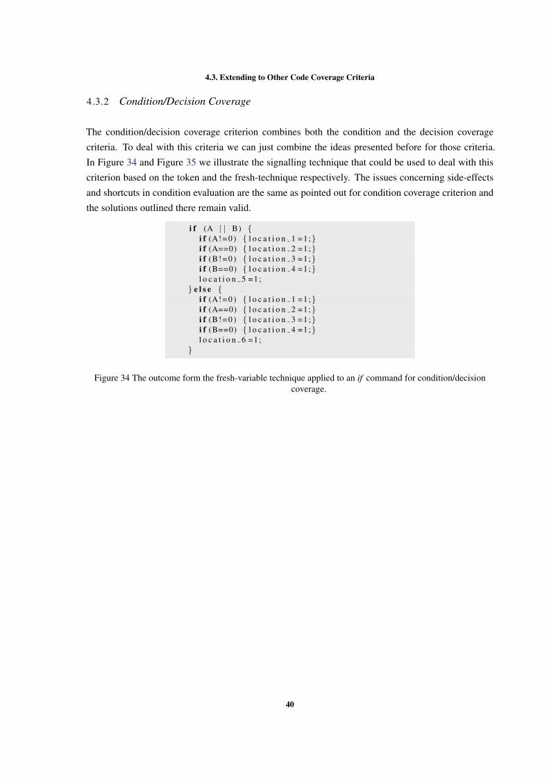
4.3. Extending to Other Code Coverage Criteria

4.3.2 Condition/Decision Coverage

The condition/decision coverage criterion combines both the condition and the decision coverage

criteria. To deal with this criteria we can just combine the ideas presented before for those criteria.

In Figure 34 and Figure 35 we illustrate the signalling technique that could be used to deal with this

criterion based on the token and the fresh-technique respectively. The issues concerning side-effects

and shortcuts in condition evaluation are the same as pointed out for condition coverage criterion and

the solutions outlined there remain valid.

i f (A | | B) {i f (A! = 0 ) { l o c a t i o n 1 =1;}i f (A==0) { l o c a t i o n 2 =1;}i f (B! = 0 ) { l o c a t i o n 3 =1;}i f (B==0) { l o c a t i o n 4 =1;}l o c a t i o n 5 =1;

} e l s e {i f (A! = 0 ) { l o c a t i o n 1 =1;}i f (A==0) { l o c a t i o n 2 =1;}i f (B! = 0 ) { l o c a t i o n 3 =1;}i f (B==0) { l o c a t i o n 4 =1;}l o c a t i o n 6 =1;

}

Figure 34 The outcome form the fresh-variable technique applied to an if command for condition/decisioncoverage.

40

4.3. Extending to Other Code Coverage Criteria

i f (A | | B) {

# i f d e f A s s e r t 1i f (A! = 0 ) { a s s e r t ( 0 ) ;}

# e n d i f# i f d e f A s s e r t 2

i f (A==0) { a s s e r t ( 0 ) ;}# e n d i f# i f d e f A s s e r t 3

i f (B! = 0 ) { a s s e r t ( 0 ) ;}# e n d i f# i f d e f A s s e r t 4

i f (B==0) { a s s e r t ( 0 ) ;}# e n d i f# i f d e f A s s e r t 5

a s s e r t ( 0 ) ;# e n d i f

} e l s e {# i f d e f A s s e r t 1

i f (A! = 0 ) { a s s e r t ( 0 ) ;}# e n d i f# i f d e f A s s e r t 2

i f (A==0) { a s s e r t ( 0 ) ;}# e n d i f# i f d e f A s s e r t 3

i f (B! = 0 ) { a s s e r t ( 0 ) ;}# e n d i f# i f d e f A s s e r t 4

i f (B==0) { a s s e r t ( 0 ) ;}# e n d i f# i f d e f A s s e r t 6

a s s e r t ( 0 ) ;# e n d i f

}

Figure 35 The outcome form the token technique applied to a if command for condition/decision coverage

41

5

A u T G e n - C T O O L

AuTGen-C was the name given to the code coverage tool developed in the context of this thesis. This

tool applies the methodologies described in Chapter 4 to programs written in ANSI-C. In this chapter

we present AuTGen-C as well as the challenges we encountered during its development. In particular,

we discuss the design choices, how we have implemented the key topics described in the previous

chapters, the challenges founded and the solution for those challenges.

Even before we started the implementation itself, an important decision had to be made. The choice

of the programming language to be used in the tool implementation. This choice must contemplate

the challenges that may appear. One relevant criterion is that the language chosen offers a parser for

the input programs to which we intend to generate tests. if this not the case a parser must be developed

from scratch, which might delay the tool development duo to the complexity of the input language.

Depending on the methodology selected, the tool executes differently. The tool is divided in differ-

ent process, each one with its own task. They are presented in Section 5.1 and debated in the follow

section. Also in a tool such as ours is essential to debate and define the concept of unit implemented

by us and introduce how can be use the tool we developed in Section 5.6 and Section 5.7 respectively.

5.1 ARCHITECTURE AND IMPLEMENTATION CHOICES

In this section we focus on the architecture of the tool. We start by discussing the chosen implementa-

tion language and the chosen libraries. We finish the section presenting the tool architecture.

5.1.1 Tools, Language and Libraries

Haskell was the programming language selected to implement the tool. Haskell1 is a purely functional

programming language with polymorphic and a monadic system. Some of its features include pattern

matching, list comprehensions and modularity. Its programming paradigm is ideal for parsing and

instrumenting abstract syntax trees which are strong topics in this dissertation. Comparatively to

others functional programming languages such as OCaml2 our programming experience using Haskell

1 http://www.haskell.org2 https://ocaml.org/

42

5.1. Architecture and Implementation Choices

was a decisive fact in the selection. Moreover, the language is supported by a big community and a

large diversity of libraries, which include libraries for parsing and manipulating C program language.

After choosing the programming language, we had to select libraries to help us develop our tool.

First of all, we had to select a parser for C programs. Here, due to the lack of alternatives we have

chose Language.C3. Such a library allows us to parse C programs and to instrument them as described

in Section 5.3. Another important library used during the development process was Text.XML.HXT4,

which allows us to parse the XML document returned by the bounded model checker.

The CBMC was the chosen bounded model checker. Our choice was influenced by investigation

developed in [2] and our experience using it. Moreover, the CBMC is one of the most used bounded

model checkers for C code programs and also contains a large diversity of documentation. Initially

we started by using CBMC 4.0. However, as CBMC was updated, we also updated our tool to be

able to interact with the most recent release of CBMC. Currently we are supporting CBMC 5.0 which

includes many improvements relatively to the initial version.

The operating system used during development was Ubuntu 12.04 LTS running on 1.8Ghz dual

core processor machine with 4GB of RAM memory.

5.1.2 Architecture and Source Code Structure

Let us now describe how the tool is implemented. The tool architecture is composed by different

components. All methodologies have in common the pre-instrumentation and test vector extraction as

is shown in Figure 36. In the figure it is also possible to observe that the coverage analysis is also the

same for all methodologies.

Figure 36 Tool architecture

3 https://hackage.haskell.org/package/language-c4 http://hackage.haskell.org/package/hxt

43

5.1. Architecture and Implementation Choices

The organisation of the code is shown in Figure 37. The main function is declared in the Main.hs

file and starts by interpreting the input options followed by the test generation itself.

Apart from the Main.hs, the main directory also contains Opts.hs, Automation.hs and Configura-

tions.hs files and some directories. All these files contains auxiliary functions which are called by

the Main.hs file. The Opts.hs file contains all the subroutines responsible for interpreting the input

options. The Configurations.hs contains the parametrizable values accessed over the several phases.

Finally, the Automation.hs file contains the auxiliary function that initializes test generation itself.

The code instrumentation is the first process executed by the tool. This step is divided in the pre-

instrumentation process and the signalling technique application process.

All the functions related to the pre-instrumentation are in PreImplementation directory. This di-

rectory contains the automation process responsible for the non-deterministic attributions, variable

declarations and initialization, function declaration and for extracting information from the code that

will be used in the following steps.

Depending on which methodology is being applied, one of the two signalling techniques is used. All

the functions related to the application of one of this techniques are in Instrumentation directory. The

Instrumentation/Coverage/StatementDecisionCoverageToken.hs, is related to the token technique and

the Instrumentation/Coverage/StatementDecisionCoverage.hs to the fresh-variable technique. Both

are called by Instrumentation/Automation.hs that contains automations responsible for applying the

coverage.

After the locations are marked in the code the test generation procedure follows. In the case of

fresh variable methodology for multi-locations the sets of locations are created, and only then the test

generation procedure starts. All the functions related to the sets of locations generation are in the

PathSet directory.

The test generation procedure includes the process of storing the generated tests, establish which

still need to be reached, manage the bound incrementation and calling the CBMC. All function related

to this procedure are in the the TestGeneration directory and each methodology have its own automa-

tion. The TestGeneration/Token/Automation1.hs file contains the function for the automation related

to the token methodology. The TestGeneration/Variables/Automation2.hs and TestGeneration/Vari-

ables/Automation3.hs files contain the function for the automation related to the variable methodol-

ogy. It is also during this process that the necessary information for calculating the level of coverage

is obtained.

Upon the conclusion of test generation procedure, the traces produced still need to be transformed

into test vectors. The functions responsible for transforming the traces in to test vectors are in the

TestGeneration/TraceParse.hs and XML/XmlCBMC.hs files.

Two other directories, not yet referred, are the Pretty and Types. They contains function related to

types transformation and types declarations required by other components.

44

5.2. Pre-Instrumentation

AuTGen-C Files

Main.hsOpt.hsAutomation.hsConfigurations.hsInstrumentation/

Automation.hsCoverage/

StatementDecisionCoverage.hsStatementDecisionCoverageToken.hs

PathSet/Convert.hsPathSetCreation.hs

PreInstrumentation/Automation.hsExternalFunctionDeclaration.hs

FunctionDependencies.hsFunctionVars.hsGlobalVars.hsStatementsAssiments.hsStatementsDeclarations.hsStatements.hsStatementsUtill.hsUtil.hsVariables/

LocationVars.hsPretty/

Pretty.hsTest.hs

Types/Annotations.hs

AST.hsCGF.hsEqUtil.hsOption.hsPaths.hs

TestGeneration/TraceParse.hsToken/

Automation1.hsVariables/

Automation2.hsAutomation3.hsStatements.hsTest.hs

XML/XmlCBMC.hs

Figure 37 Structure of the tool filesystem

5.2 PRE-INSTRUMENTATION

The first process shown in the tool architecture(Figure 36) is the pre-instrumentation. However, for

this process to be possible the tool has first to perform some standard tasks, such as, for instance, parse

the input program and interpret the user input options (command line flags). We omit a description

about these implementation details because they are standard tasks performed by any regular tool.

Nonetheless, it is important to note that after these tasks are performed one obtains an AST with the

input program and another structure with the selected options.

One of options that the user has to specify is the name of the target function (as well as the file name)

to be used as entry point for the generated tests. The arguments of this function must be modelled in

a way that the test vectors generated contains possible user inputs, as explained in Section 3.2.1.

The principal idea of the pre-instrumentation is exactly to model the arguments of the target func-

tion. A new main function is created whose purpose is to call the target function with the modelled

arguments. For each argument, we analyse its type and assign to it an arbitrary value. In CBMC

this can be done by assigning to a certain variable the result of an external function whose return type

matches the variable type. Predefined external functions exist in CBMC (such as the int nondet_int

();) and those do not have to be declared. If the assignment x = nondet_int(); takes place, CBMC

will consider that x has an arbitrary value. As an example see how variable show_help is assigned in

Figure 38.

If a predefined external function is not provided by CBMC, it can just be declared. This is particeu-

larly useful for user defined structures. Figure 38 shows the declaration of an external function that

returns a struct stat. This function is then used to assign an arbitrary value to variable out_stat.

45

5.2. Pre-Instrumentation

e x t er n s t r u c t s t a t n o n d e t s t r u c t s t a t ( ) ;

i n t main ( ) {i n t show he lp ;s t r u c t s t a t o u t s t a t ;o u t s t a t = n o n d e t s t r u c t s t a t ( ) ;show he lp = n o n d e t i n t ( ) ;

. . .

Figure 38 Part of program emphasizing non-deterministic initialization

L I M I TAT I O N I N T H E M E T H O D The method described previously has some limitations due to the way

CBMC presents counter-examples. For variables declared as pointers, CBMC only shows the address

of that pointer and not the content in that address. Certainly a content value was taken into account

during the model checking process which might have been crucial for detecting the counter-example

generated. Unfortunately, CBMC does not shows it in the returned counter-example. Consider the

example in Figure 39. If CBMC returns a counter-example the value of *aux will not be visible.

i n t f ( i n t ∗x ) {. . .

}

e x t er n i n t ∗ n o n d e t i n t p o i n t e r ( ) ;

i n t main ( ) {i n t ∗ a r g = n o n d e t i n t p o i n t e r ( ) ;f ( a r g ) ;

}

Figure 39 Part of program emphasizing an alternative initialization method

We try to resolve this issue using auxiliary variables. For the example in Figure 39, we would

declare a new variable int aux = *arg; to capture the value *arg as shown in Figure 40.

i n t f ( i n t ∗x ) {. . .

}

e x t er n i n t ∗ n o n d e t i n t p o i n t e r ( ) ;

i n t main ( ) {i n t ∗ a r g = n o n d e t i n t p o i n t e r ( ) ;i n t aux = ∗ a r g ;f ( a r g ) ;

}

Figure 40 Part of program emphasizing an alternative initialization method

46

5.3. Instrumentation Process for Decision Coverage

This alternative initialisation method would result if pointer only pointed to “simple” types, such as

int and char. A “complex type” is for example arrays. A variable of the type int* may point to a array

of type int. For the example in Figure 40 if the function expected an array only the first position of

the array would be recovered.

Once this alternative initialization method, for some cases, only retrieves part of the crucial infor-

mation necessary to create a test, the test created may not be lead to the program execution as intended.

Moreover, the tests created will probably introduce redundancy and reduce the percentage of coverage

achieved.

In attempt of retrieve the full information was try auxiliary variables of array type with fixed size,

once the CBMC can show correctly the values in arrays with fixed size. The example in Figure 41

is shown the aux variable as an array of size 3. Even with this change we continue with same issue.

The size use in the auxiliary array variable is not enough to retrieve the position 6, which is a crucial

for the test generation. This solution to work requires to know the correct size to be use in the aux

variable.

i n t f ( i n t ∗x ) {i f ( x [6] >3)

. . .}

e x t er n i n t ∗ n o n d e t i n t p o i n t e r ( ) ;

i n t main ( ) {i n t ∗ a r g = n o n d e t i n t p o i n t e r ( ) ;i n t aux [ 3 ] = ∗ a r g ;f ( a r g ) ;

}

Figure 41 Part of program emphasizing an alternative initialization method

As solution was not found, none of this alternatives was implemented. Also research over this topic

lead us to the information that pointer allocation and other related features are under development by

CBMC developers and is expected news over this topics in the next CBMC releases.

5.3 INSTRUMENTATION PROCESS FOR DECISION COVERAGE

Before the test generation process, the target code is instrumented for the decision criterion. The

notion of decision coverage in our tool is as follows: every decision in the program has taken all

possible outcomes at least once and every point of entry has been invoked at least once (note that

some authors defend a stronger criterion as discussed in Section 2.2.2, every point of exit must also be

invoked at least once). During this process the locations are identified and the annotations are inserted

with the corresponding signalling technique to the methodology in use. The instrumentation process

47

5.3. Instrumentation Process for Decision Coverage

starts by receiving an abstract syntax tree generated by pre-instrumented process as explained in the

previous section.

The tool has first to calculate function dependencies, according the user choice. For that, we iterate

over the abstract syntax tree and for each function call and we keep track of its dependencies.

The abstract syntax tree generated by the Language.C library does not consider directives. We

only can speculate that the reason of such a behaviour is related to the process used by the library. It

starts by invoking an external C preprocessor, which removes all directives, and only then parses the

resulting program.

In order to instrument the code using the token methodology we had to develop a solution to support

the #ifdef directive. Two possible solutions emerged. The first option was to change the abstracted

syntax tree data type and create the element corresponding to directive #ifdef.

The other option, that we ended up using, consisted in using a functionality given by the library.

The abstract syntax tree structure is created in such a way that every element in it can carry an auxiliary

parameter. The only restriction is that all auxiliary parameters must have the same type.

For both alternatives, the pretty printer component from the Language.C library would have to be

modified. Nevertheless, if the first option would have been used, we would also have to be changed

the structure provided by the library. Besides that using the second option facilitated the development

of other tasks.

The Data Supporting the Annotations

The data supporting the annotations is defined in Figure 42. The type shown contains the elements

related to the annotations used to apply both signalling techniques.

data Annotation =IFDef Int [Annotation]

| Assume Expression| Assert Expression| Label Int

Figure 42 Annotation type definition

An Annotation instance can be created by using one of four constructors. The #ifdef directive can

be created by the IFDef constructor. Its parameters are an identifier (Int) to the location in question

and a list of annotations ([Annotation]). The list of Annotation correspond to the annotations to be

inserted in the #ifdef body. The standard annotations from bounded model checkers, assume and

assert statements, can be created by the Assume and the Assert constructors. Both have as parameter

a C language expression (Expression). The Label annotation is used by fresh-variables methodologies

and represents the attribution to the variable associated to that location. Its contains a parameter

(Int) that is the identifier of the location. It is used to create the assignmentused in the fresh-variable

technique.

48

5.3. Instrumentation Process for Decision Coverage

The introduction of annotations in the abstract syntax tree

The process of inserting the required annotation for both signalling techniques only differ in the an-

notations that are inserted. This process starts by receiving the abstract syntax tree from the pre-

instrumentation process and then changes its auxiliary parameters to receive the annotations. It is also

applied some simplifications, for instance do while loops are transformed into while loops, required

by both signalling techniques.

type AuxiliaryParameter = ([Annotation],[Annotation])

Figure 43 The auxiliary variable type definition

The auxiliary parameters type used is shown in Figure 43. The AuxiliaryParameter contains two

fields, each one containing a list of Annotation. This two fields divide the annotations that must be

inserted in true and false outcome of a condition statement. The type used in the fields may be con-

sidered excessive because there exists simple types to represent the auxiliary parameter. Nonetheless,

we aimed to keep it as general as possible thinking already in the instrumentation for other coverage

criteria. For the fields that do not contain any annotation is used the empty list.

The AuxiliaryParameter instances which receive annotations are the ones which are appended to

statements related to decisions, for instance if and while statements. Depending on the signalling

technique being used is inserted the different annotations. For the token technique it is inserted the

IFDef annotation with a assert statement with the false expression (IFDef i [Assert 0]). For the fresh-

variable technique it is inserted the annotation correspondent to the variable assignment (Label i). In

both cases the i element is the location identifier.

The pretty print

When the abstracted syntax tree is pretty printed, the elements from the Annotation type must be also

printed. Each Annotation element is printed as shown in Figure 44. The e and i are the arguments

used in there construction. Also it is use the name DEFINE_ as the macro’s name in the #IFDef and

the name cc_loc_ as variables name in the variables Label.

c c l o c i = 1 ;

(a) Label

a s s e r t ( e ) ;

(b) Assert

CPROVER assume ( e ) ;

(c) Assume

# i f d e f DEFINE i/∗ A n n o t a t i o n s

p r e t t y p r i n t ∗ /# e n d i f

(d) IFDef

Figure 44 Annotations pretty print

49

5.4. Set of Locations Sets Generation

sw i t ch ( i ){case 1 :c c l o c 2 =1;case 2 :c c l o c 3 =1;

i = 0 ;d e f a u l t :c c l o c 4 =1;}

i f ( i >0){c c l o c 5 =1;

i ++;}e l s e{c c l o c 6 =1;

i−−;}

whi le ( i < 0){c c l o c 5 =1;

i ++;}c c l o c 6 =1;

Figure 45 Statements pretty print

The annotations inserted in the auxiliary parameters are placed in beginning of the corresponding

sequence of statements. In Figure 45 is shown on the left had side the example of pretty printing

an switch statement, on the middle the pretty printing of an if statement and on the right the pretty

printing of a while loop.

5.4 SET OF LOCATIONS SETS GENERATION

The set of sets generation is a process that only occurs when the fresh-variable methodology is used

for multi-locations. After the code is instrumented accordingly to the previous section, the resulting

abstract syntax tree is used to generate possible execution paths that are transformed in set of sets to

be used by the fresh-variable methodology for multi-locations.

Since the bounded model checking only checks executions within the established bound, only ex-

ecution paths within the establish bound are considered in the construction of the set of sets. The

generation of sets from execution paths outside of the established bound would be a waste of compu-

tational time as the bounded model checker cannot generate traces containing those paths.

The process of creating the set of locations starts by creating a new data structure that captures

exclusively the control flow of the initial program. Such a data structure is shown in Figure 46 and is

used to agile the set construction process. Note that at this point we know that our target program is

syntactically well constructed.

The ReducedTree a data type show in Figure 46 is the new data structure used to capture the control

flow of the initial program. For each function in the initial program a ReducedTree is constructed.

The ReducedTree a is a list of elements of data type Command a, which corresponds to a sequence of

statements from a function in the initial program.

The Command data type can be created using different constructors. The constructor C is used

when a function call is met. The constructor R, B and Cont is used whenever a return, break, or

continue statement is encountered respectively. When an assignment inserted by the instrumentation

process in the fresh-variable technique is met, the Id constructor is used. For switch statements we

use the Switch constructor and for each case we use the Case constructor. Finally for the if, and

50

5.4. Set of Locations Sets Generation

data ReducedTree a = [ Command a ]data Command a =

C name| R| B| Cont| Id a| Swi tch [ Command a ]| Case [ Command a ]| I f ( [ Command a ] , [ Command a ] )| Loop ( [ Command a ] , [ Command a ] )

Figure 46 The commands in the reduced abstract syntax tree

while statement, the If and Loop constructors are respectively used. Note that the Switch and Case

constructors have also one argument used to capture their content. The same applies to the If and

Loop, but in these cases, both have two arguments: one for the case in which the condition is true and

another for the case in which the condition is false.

/* The cc_loc_* are thevariables signalizing thelocations */

int trap(int a){cc_loc_1 =1;while (a < 6){cc_loc_2 =1;if (a % 2){cc_loc_3 =1;a++;

} else {cc_loc_4 =1;a = a + 2;

}}cc_loc_5 =1;return a;

}

Figure 47 The trap function instrumented using the fresh-variable technique

An example of a ReducedTree instance corresponding to the code shown in Figure 47 is [Id 1,Loop

([Id 5],[Id 2,If ([Id 3],[Id 4])]),R]. Note that the assignments represented in the program

as a++ and a = a + 2 are not captured in this new representation, but the special assignments (which

in reality are just auxiliary parameters in the AST) are captured.

To transform a ReducedTree into to set of locations sets, for each instance of the ReducedTree.

From there, the process goes backwards until the first element in the list. To evaluate the last element,

an empty set is received corresponding to the possible execution paths from that point onwards. The

51

5.5. Test Generation and Test Vector Extraction Processes

result of evaluating the last element is propagated to the evaluation of the previous. The process

follows like this until the first element.

Note also that some instances of the ReducedTree can have arguments. Those will originate differ-

ent set of locations. For instance, the evaluation of an the command If ([Id 1],[Id 2]) will result

in the following set: {{1},{2}}. If instead we have another location before the if, such as [Id 3,

If ([Id 1],[Id 2])] the result of the If command will be propagated backwards, resulting in the

following set: {{3,1},{3,2}}.

A special case of this evaluation is the Loop constructor. In this case, one must consider the result

of multiple iterations. For that we start by creating a set of locations corresponding to the loop body,

and after that we apply the cartesian product as many times as the chosen bounded (this is the same

value given to the BMC tool).

Other constructors with special semantics is the R, B and Cont. Note that the R constructors corre-

sponds to the return statement. That means that whenever an R instance appears the execution of that

function must stop, and therefore all subsequent executions paths must be ignored. The B constructor

represents the break statement and therefore, the subsequent commands in the same scope must be

ignore, making the execution continue in the next scope. Finally the Cont constructor, corresponding

to the continue statement has only to ignore the subsequent commands in the current execution. Note

that these constructors must be evaluated first, in order to capture the described behaviour.

Another command requires special attention is the goto statement. This command is not supported

in the current version of the tool. Such could be implemented by having a set of locations associated

to each label. This way, each time a goto label_1; is found we combine the current set with the set

associated to the label_1.

The set of locations obtained from this procedure are then used by the fresh-variable methodology

for multi-locations as explained in Section 4.2.3.

5.5 TEST GENERATION AND TEST VECTOR EXTRACTION PROCESSES

As explained previously, for the generation of set of tests we use CBMC. In this section we describe

how to interact with CBMC to perform bounded model checking of software to the instrumented file.

Moreover, we also describe how to interpret the results given by CBMC to create a set of tests.

5.5.1 CBMC Interaction and Test Construction

The interaction between our tool and the CBMC tool is done through system calls. Every time the

tool needs to perform bounded model checking to an instrumented program and produce a test case

we print the program to a file and invoke CBMC through a system call. The CBMC outputs the result

to the standard output which is then interpreted by our tool.

52

5.5. Test Generation and Test Vector Extraction Processes

The performed system call has the following format: cbmc -D <macro> <file-name> --unwind

<number> --no-unwinding-assertions --xml-ui, where the option -D <macro> is only used when

the token methodology is being used (more details are given in Section 3.2.1). The option --xml-ui is

used for CBMC to use a XML file as output. Such facilitates the interpretation of results and creation

of tests.

We use the Text.XML.HXT library to parse the CBMC output file. Such a file includes a trace that

leads to an assertion violation. In our case, such a trace, represents exactly an execution going through

the locations we specified. In simplified terms, a trace corresponds to the evolution of the variables

along the execution of the program. Figure 48 shows part of a trace. In particular it shows the result

of an assignment to variable cc_loc_3 (an auxiliar variable introduced in the pre-instrumentation

process). From the XML element it is possible to extract different information, such as, for instance,

the type of the variable, the file and the line in which it appears, and the value that is assigned to the

variable.

<a s s i g n m e n t a s s i g n m e n t t y p e =” s t a t e ” base name =” c c l o c 3 ”d i s p l a y n a m e =” c c l o c 3 ” h i dd en =” f a l s e ” i d e n t i f i e r =” c c l o c 3 ” mode=”C”s t e p n r =”72” t h r e a d =”0”>< l o c a t i o n f i l e =” I n s t r u m e n t e d C o d e . c ” f u n c t i o n =” f ” l i n e =”15”/><type>i n t </ type>< f u l l l h s >c c l o c 3 </ f u l l l h s >< f u l l l h s v a l u e >1</ f u l l l h s v a l u e ><va lue >1</ va lue><v a l u e e x p r e s s i o n >

< i n t e g e r b i n a r y =”00000000000000000000000000000001” c t y p e =” i n t ”wid th =”32”>1</ i n t e g e r >

</ v a l u e e x p r e s s i o n ></ a s s i gnmen t>

Figure 48 XML assignment

The require information to be extracted, from each trace, may change depending on the method-

ology in use. Something that is common to all techniques is the initial values of the function input

arguments. Those are going to be used in the generated test. Moreover, it is important to extract the

locations that were reached with the current execution. All this information is easily accessible in the

XML file. It consists mainly in reading the carry by the variables. The reached locations are identified

by observing whether the variable associated to a location was attributed or not. The values attributed

to the arguments of the target function are obtained by filtering all the attributions in the main function

and the selecting the ones used to call the target function.

The reached locations are identified by observing whether the variable associated to a location was

attributed or not. The values attributed to the arguments of the target function are obtained by filtering

all the attributions in the main function and the selecting the ones used to call the target function.

With the information extracted from the traces produced by CBMC we produce the set of tests

which are then stored in a file. Figure 49 shows an example of such a file. Each line represents a test

53

5.6. The Unit Used

input case, and within each line we have the values that are assigned to each variable. More concretely

each line is composed by the argument type, name and the value it takes on that test.

1 i n t i 257702809 , i n t j 0 , i n t k −257702802;2 i n t i −634666905 , i n t j 1281384480 , i n t k 1254105088;3 i n t i −760495001 , i n t j −760495001 , i n t k −1901164487;4 i n t i 671420665 , i n t j 134545163 , i n t k 671420665;5 i n t i 761215897 , i n t j −1387703479 , i n t k −1387703479;6 i n t i 1512386809 , i n t j 1512386809 , i n t k 1512386809;7 i n t i −770980761 , i n t j −2025477607 , i n t k −1531138496;8 i n t i −729562009 , i n t j 1077944352 , i n t k 1077944352;

Figure 49 Test vectors file

5.5.2 CBMC Limitations

When using CBMC as an auxiliary tool for generating tests, we are fronted with some limitations. In

our point of view, the tool should allow for the user to verify only the inserted properties. Unfortu-

nately this is not possible and CBMC always inserts some properties to be later verified. This behavior

can lead to the generation of counter-example traces that are not related to test generation process, but

else to the violation of CBMC inserted assertions.

An alternative we had to consider in order to avoid the properties inserted by CBMC was to use the

command line flag --property N. The behavior of this flag is that CBMC will only take verify the

property number N. Note that a value is assigned to each property by CBMC, and therefore, we must

make sure that we are checking the correct property.

The value associated by CBMC to the assert responsible to trigger the trace generation when use the

fresh-variable technique is always the same. However, this behaviour, by the CBMC, is not observed

when use the token technique.

5.6 THE UNIT USED

To allow the tool to adapt to the criterion that an user may have as unit, we developed three criteria

from which the user may choose. The first one will cover the target function and all the function

that may be executed from the target function. The second criterion only covers the target function.

And the third criterion covers the target function and the functions indicated by the user. This three

alternatives were named as dependency unit, single unit and selected unit respectively.

Consider the example, shown in Figure 50, where the function A calls the functions B and C, and

the function C calls D. If the function a was selected as target function, for the first alternative the

locations from A, B, C and D would be taken in consideration. For the second alternative only the

54

5.7. Tool Guide

Figure 50 The function dependencies

function A would be consider and for the third alternative A and the ones indicated by the user would

be consider.

5.7 TOOL GUIDE

In this section we present a tutorial about the tool usage. We cover different ways of invoking the tool,

by showing the command flags that must be provided to it. Moreover, we show how to use different

methodologies and different units.

A S I M P L E C A L L

AuTGen-C -t <function-name> <file-name>

This is the simplest way of invoking the tool. The option -t follow by the function name is used to

indicate the target function. By default, this command will apply the fresh-variable methodology for

single location with a initial bound of one and a maximum bound of five. The unit us by default is the

dependency unit.

E S TA B L I S H T H E I N I T I A L A N D M A X I M U M B O U N D

AuTGen-C -t <function-name> <file-name> -s <number> -m<number>

The command line flags -s and -m can be used to indicate respectively the minimum and maximum

bound.

T H E U N I T T Y P E S E L E C T I O N

AuTGen-C -t <function-name> <file-name> --uDepend

AuTGen-C -t <function-name> <file-name> --uSingle

AuTGen-C -t <function-name> <file-name> --uSelect -f<function-name>

To select the kind of unit the user is interested to cover, the command line flags --uDepend, --

uSingle and --uSelect can be used. When the first is used, the dependency unit is used. When the

second is used, the single unit is used and finally, when the last is used the user can provide the

functions to be covered as parameters through the flag -- f , one for each function the user wants to

add.

55

5.7. Tool Guide

T H E M E T H O D O L O G Y S E L E C T I O N

AuTGen-C -t <function-name> <file-name> --decision token

AuTGen-C -t <function-name> <file-name> --decision single

AuTGen-C -t <function-name> <file-name> --decision multi

To select the methodology to be used, the --decision command flag can be used, together with a

parameter: token for the token methodology; single for the fresh-variable methodology with single

location; multi for the fresh-variable methodology with multi location.

OT H E R O P T I O N S

AuTGen-C -t <function-name> <file-name> -v

AuTGen-C -t <function-name> <file-name> -h

Finally, as usual, the command line flags -v and -h can be used to show respectively the version of

the tool and some helpful information.

56

6

E VA L UAT I O N A N D C O N C L U S I O N S

In this section we evaluate our tool, and provide an overview of its capabilities. Moreover, we perform

an empirical study comparing the different methodologies using different case studies. We start by

presenting the results obtained by running our tool, using different methodologies, with different

algorithms and then we make a global analysis of the tool. We finish this chapter and this dissertation

with some conclusions and some ideas for future work.

6.1 TOOL EVALUATION

The first two case studies were previously used to validate LocFaults tool [4] and are available from

http://www.i3s.unice.fr/˜bekkouch/Benchs_Mohammed.html. The first case study is a C imple-

mentation of the famous bubble sort ordering algorithm and the second, which we will call maxmin6,

is an implementation of an algorithm that calculates the maximum and the minimum value of six

variables.

The third case study, called cars, was previously used as a benchmark in [10] and is available

from https://bitbucket.org/vhaslab/benchmarks/src/4978b4b15bb2/dagger/ORIGINAL/. Fi-

nally the last case study we consider is the grep utility version 2.21 from unix system, whose source

code is available from ftp://ftp.gnu.org/gnu/grep/.

Each one of this case studies was selected because they contribute to different aspects of the evalua-

tion. The bubble sort function contains two nested loops, the maxmin6var function contains no loops,

the cars function contains non-deterministic functions that determines the outcome of decisions and

the grep utility is a large real world application (contains more than 2000 lines of code) and therefore

allows us to observe how the tool scales.

For each case study, we run our tool multiple times changing only the lower and upper bound.

Moreover, for each bound interval, we run it with the different methodologies. The tables containing

the results are divided into groups and each group contains the different methodologies with the same

bound interval and unit used.

With respect to the columns, we present the following information:

- Methodology: the methodology in use;

57

6.1. Tool Evaluation

- Computation Time / CPU Time: total time, and time omitting the CBMC computation time;

- Number of locations to reach: total number of locations;

- Code coverage: percentage of code that has been reached;

- Number of tests: number of generated tests;

- Missed locations: the locations that were not reached by any test;

- Infeasible set of locations: number of set of locations that have been generated and tried but

were infeasible.

Bubble Sort

BubbleSort

Boundrange Methodology

ComputationTime / CPU

Time

Number oflocations to reach

Percentageof coverage

reached

Number oftests

Missedlocations

Infeasible setof locations

searched

[min

:1m

ax:1

] Token 2s / 0.54s 7 71% 5 [2,4]

Fresh-VariableSingle location

2s / 0.03s 7 0% 0 all

Fresh-VariableMulti-location

1s / 0.02s 7 0% 0 all 4

[min

:9m

ax:9

] Token 4s / 0.70s 7 71% 5 [2,4]

Fresh-VariableSingle location

3s / 0.14s 7 0% 0 all

Fresh-VariableMulti-location

1s / 0.09s 7 0% 0 all 5

[min

:16

max

:16] Token 6s / 2.18s 7 100% 7 none

Fresh-VariableSingle location

2s / 1.12s 7 100% 1 none

Fresh-VariableMulti-locations

2s / 1.23s 7 100% 1 none 0

[min

:1m

ax:1

6] Token 14s / 2.48s 7 100% 7 none

Fresh-VariableSingle location

7s / 1.38s 7 100% 1 none

Fresh-VariableMulti-locations

7s / 1.47s 7 100% 1 none 0

Table 1 The bubble sort evaluation results

This case study consists of a bubble sort algorithm implemented for arrays with 16 elements. Note

that for a lower and upper bound of one the token methodology is already able to reach 71% of

decision coverage, failed only to coverage two tests. However, for the other methodologies, tests are

not generated.

When we set the upper bound to 16, all methodologies are able to generate tests which reach 100%

of decision coverage. Nonetheless in this case, we can observe that when using the methodologies

58

6.1. Tool Evaluation

based on the fresh-variable technique only one test is generated and the token methodology generates

seven tests. Taken in account the case study, we can affirm that six of seven tests generate by token

methodology are redundant.

With respect to the execution time, the token methodology is always slower. It is with initial and

maximum bound of sixteen that the disparity in execution time of the methodologies is greater. We

can also observe a scale in execution time when used the initial bound of one and max bound of

sixteen comparatively to the use of initial and maximum bound of sixteen.

With respect to the execution time, the token methodology is always slower. Note in particular the

high values in the case in which the lower bound is 1 and the upper bound is 16. This will make

that our tool will first try to cover all locations with a bound 1 when calling CBMC, and then if some

location is still not reach with the produced tests, it will increase the bound until all locations are

reached or it reaches the bound 16. This case studies requires a minimum bound of 16 to cover all

locations, therefore, it is more efficient if one starts to consider the minimum bound of 16.

Maximum and minimum of six variables

Maxmin6var

Boundrange Methodology

ComputationTime / CPU

Time

Number oflocations to reach

Percentageof coverage

reached

Number oftests

Missedlocations

Infeasible setof locations

searched

[min

:1m

ax:1

] Token 16s / 2.12s 59 100% 59 none

Fresh-VariableSingle location

12s / 2.68s 59 100% 30 none

Fresh-VariableMulti-location

12s / 2.68 59 100% 30 none 0

Table 2 The maxmin6var evaluation results

As expected, since this case is absent from loops, all three methodologies reached 100% of code

coverage only with lower and upper bound of one. The token methodology generates fifty nine tests

and the methodologies based on the fresh-variable technique generate only thirty tests.

Even if we try to increment the lower and upper bound, the number of generated tests and the time

spent will be exactly the same, because our tool will stop as long as all locations are reached and in

terms of CBMC it has no difference because do no exist loops.

59

6.1. Tool Evaluation

Cars

Cars

Boundrange Methodology

ComputationTime / CPU

Time

Number oflocations to reach

Percentageof coverage

reached

Number oftests

Missedlocations

Infeasible setof locations

searched

[min

:1m

ax:1

] Token 7s / 0.75s 26 88% 23 [19,22,25]

Fresh-VariableSingle location

4s / 0.48s 26 77% 8[

17, 19, 21,22, 23, 25

]Fresh-VariableMulti-location

3s / 0.48 26 77% 8[

17, 19, 21,22, 23, 25

]5

[min

:2m

ax:2

] Token 8s / 0.75s 26 88% 23 [19,22,25]

Fresh-VariableSingle location

5s / 0.57s 26 88% 9 [19,22,25]

Fresh-VariableMulti-location

6s / 0.61s 26 88% 9 [19,22,25] 8

[min

:10

max

:10] Token 9min / 0.8s 26 88% 23 [19,22,25]

Fresh-VariableSingle location

3min / 0.79s 26 88% 10 [19,22,25]

Fresh-VariableMulti-locations

7min / 0.83s 26 88% 9 [19,22,25] 12

[min

:1m

ax:1

0]

Token 12min /0.93s

26 88% 23 [19,22,25]

Fresh-VariableSingle location

6min / 0.76s 26 88% 9 [19,22,25]

Fresh-VariableMulti-locations

14min /1.31s

26 88% 9 [19,22,25] 12

Table 3 The cars evaluation results

The cars case study consists in a function relating three cars, more specifically, their positions and

velocities in different time intervals. In each interval the car position is updated depending on the

current speed and the velocity might be non deterministically updated.

As we can observe in Table 3, the token methodology performs better when using 1 as lower and

upper bound. It can reach 88% of decision coverage, while the other two methodologies reach only

77%.

With respect to the number of generated tests the token methodology is the less efficient. Twenty

three tests are generated as opposed to nine in the methodologies based on the fresh-variable tech-

niques for the same result in terms of coverage level.

In general, the methodology which is less time efficient is the token methodology. Something worth

to be mentioned is the performance by the fresh-variable methodology for single location when we

set the lower and upper bound to ten. It is twice as fast as the fresh-variable methodology for multiple

location and three times faster than the token methodology.

60

6.1. Tool Evaluation

Grep

GrepBoundrange /Unit

MethodologyComputationTime / CPU

Time

Number oflocations to reach

Percentageof coverage

reached

Number oftests

Missedlocations

Infeasible setof locations

searched

[min

:0m

ax:0

]Si

ngle

Uni

t Fresh-VariableSingle location

40mins /9.85s

59 79.66% 12 (12)1

Fresh-VariableMulti-location

30min /8.25s

59 55.93% 7 (26)1 32

[min

:1m

ax:1

]Si

ngle

Uni

t Fresh-VariableSingle location

43mins /9.99s

59 79.66% 12 (12)1

Fresh-VariableMulti-location

[min

:0m

ax:0

]D

epen

denc

yU

nit

Fresh-VariableSingle location

146mins /44.15s

306 68.62% 34 (96)1

Fresh-VariableMulti-location

37min /9.63s

306 27.77% 7 (221)1 32

[min

:1m

ax:1

]D

epen

denc

yU

nit

Fresh-VariableSingle location

146mins /44.28s

306 68.62% 34 (96)1

Fresh-VariableMulti-location

Table 4 The grep evaluation results

The grep utility is a unix command line tool that prints each line of a text that contains a certain

pattern. Its implementation has roughly 2500 lines of code.

To evaluate the grep utility, we had to gather all code into a single file - this is a current restriction of

our tool. Moreover, as we have explained inSection 5.5.2, due to CBMC restrictions we were not able

to test the token methodology and ended up testing only the methodologies based on the fresh-variable

technique. The first two groups of lines in Table 4 are assuming single unit when calculating the level

of coverage and the other two groups are assuming dependency unit - see discussion in Section 5.6.

The grep function in grep utility is being used as the target function.

From the Table 4, we can observe that the fresh-variable for multi-location methodology does not

scale even for the case in which loops are unwind only once. In the case of single unit the tool was still

able to generate the set of locations, but then it was unable to terminate the computation to generate

tests in less then 24 hours. In the case of dependency unit, the tool was unable to generate the set of

locations.

If one considers an isolated function to be the smallest unit in a system and if the fresh-variable for

single-location is used, the tool is able to reach almost 80% of decision coverage in the case of the

1 Number of locations that were not reached

61

6.2. Global Analysis

grep function (shown in the first line of the table). This value is kept even if the tool unwinds loops

once (shown in the second line of the table). In the case of fresh-variable for multi-location the tool is

only able to reach 55.3% of decision coverage if loops are not unwound.

When considering the dependency unit as the criterion, we are able to reach more 68% of decision

coverage even if loops are not unwound. This means that almost 69% all locations in the grep function

and in the functions that are invoked through function calls are reached. Nonetheless, when using the

fresh-variable for multi-location, the tool only covers 27.77% of the code.

6.2 GLOBAL ANALYSIS

In the previews section, we made some observations about the results obtained for each case study

separately. In this section we make a global analysis taking into account all the cases studies and

making some observations about the results we obtained.

The first thing worth of note is that the token methodology can reach higher levels of decision

coverage with smaller bounds than the methodologies based on the fresh-variable technique. The

explanation for this behaviour is that the execution traces produced by CBMC do not need to reach

the end of the program. On contrary, when using the methodologies based on the fresh-variable

technique, the produced traces need to reach the end of the program. See Section 4.1, where both

techniques are described. The bubble sort case study is excellent example as it requires at least 16

iteration so the CBMC be able to produce a trace using the fresh variable technique.

Besides the previous limitation, the methodologies based on the fresh-variable technique are more

time efficient and also produce less redundant tests. The case study that clearly shows this behaviour

is the bubble sort function - the methodologies based on the fresh-variable technique generate only

one test that reaches all locations. On the other side the token methodology produces as many tests

as the number of locations - seven in total. Nonetheless, the same behaviour is observed in the other

case studies.

For the first three case studies, when comparing the methodologies based on the fresh-variable

technique we cannot see much difference. Both methodologies generate slightly the same number

of tests in the same period of time. However, when looking at the fourth case study we can observe

that the fresh-variable for multi-location did not scale for long execution runs, as it is the case when

the tool unwinds loops once. Note also that when the technique is able to generate tests, those do

not reach the same level of coverage as the tests produced by the fresh-variable for single-location.

However, we should note that this is not a limitation of the methodology. Instead it is a limitation of

the current implementation because we are still not supporting goto statements. When creating set of

locations we just ignore the semantics of the goto statements.

62

6.3. Conclusion

6.3 CONCLUSION

The main contribution of this dissertation is the release of an automated test data generator for pro-

grams in C language using the software bounded model checker CBMC. Initially we aimed to extend

the methodology presented in Angeletti et al. [2], by generating tests to reach other coverage criteria

(the methodology presented in [2] only supports decision coverage). However, due to some setbacks,

we ended up focusing on improving the methodology to generate tests to reach decision coverage

and we only discuss how the condition coverage and condition/decision coverage criteria could be

implemented. We ended up with three different methodologies. Comparatively to the methodology in

presented [2], our methodologies do not relay on the use of code coverage analysis tools.

Initially, we tried to reproduce the methodology described by Angeletti et al. [2]. However, we

did not find a suitable external coverage analysis tool and ended up developing the so called token

methodology. This methodology differs from the original in some aspects. As opposed to the original

technique, our technique always generate as many tests as the number of locations to be reached. This

happens because the original technique depends on an external tool, and once the external tool signals

that all locations were reached the test generation process can stop. However, both this methodologies

obtains the same results (in time, tests, and coverage achieved) whenever the original methodology

has no need to call the external tool or whenever the token methodology has no need to increase the

bound.

The results produced by the token methodology did not satisfy us. The only way to improve the

results would be through knowledge of the locations achieved by each test. To solve such matter,

we developed a new technique to signalize the locations, which we end up calling the fresh-variable

technique. Based in this technique, we developed other two new methodologies, the fresh-variable for

single location and the fresh-variable for multi-locations, which were implemented in our tool.

Both methodologies based on the fresh-variable technique produce similar results and perform

significantly better than the token methodology in the cases that the considered bound allows for full

executions to be considered. Note that when using the fresh-variable technique only traces containing

a complete path of the target function are returned by CBMC. When using the signalling technique

from the token methodology, the execution traces do not necessarily need to reach the end of the

program. Also recall that the results obtained when the fresh-variable technique is applied are highly

dependent on the way that locations or set of locations are chosen. Implementing heuristics can

lead improvements on the number of generated tests and also on their redundancy. For instance, for

the fresh-variable methodology using single location, we used the heuristic that chooses the deeper

location in the program structure and also the one that is in the last part of the program. We observed

that if we changed the heuristic applied, for instance to select the location placed first in the code, the

number of generated tests increases and as consequence the number of redundant tests also increases.

The grep utility evaluation intended to test the tool capability and effectiveness in large and com-

plex applications source code. Unfortunately, due to CBMC restrictions, we were not able to use the

63

6.4. Future Work

token methodology and ended up using only the methodologies based on the fresh-variable technique.

Although we only used small bounds due to state space explosion, we managed to obtain high percent-

age of code coverage. For less complex code, the tool performed very well obtaining 100% of code

coverage code coverage for the exception of the cars function which failed to reach three location

we believe to be unreachable (actually CBMC failed to find execution traces reaching those locations

even when we set the bounds up to 200).

6.4 FUTURE WORK

We have developed the AuTGen-C tool which is available and ready to be used. The preliminary

experiments with our case studies were very encouraging, but there are still some features that can be

improved.

In the current version of the tool the fresh-variables methodology for multi-locations does not deal

with goto statements. We did not implement that for lack of time, but we do not anticipate major

difficulties in doing that.

Another feature to be implemented in a future version of the tool is the generation of tests for other

coverage criteria. We have addressed this topic in Chapter 4, concerning condition and condition/de-

cision coverage, but a more detailed study has to be done before the implementation.

Despite the success of the experiments with the case studies here described, further experiments

should be carried out with different kinds of C programs and with C programs of bigger dimension.

Moreover, we should also make a study comparing the AuTGen-C tool with other existing tools of

test data generation for C programs. The lessons learned from that study should guide other possible

improvements for the AuTGen-C platform.

Another line of work is to analyse the quality of the tests generated by the different methodolo-

gies implemented in the tool and to propose improvements to the algorithms in order to minimize

the number of tests generated without losing coverage. In particularly, we should investigate new

methodologies, based in the fresh-variable technique, with the aim of producing set of tests without

redundancy.

An interesting feature to be added to this tool is the automatic inference of the minimum bound to

achieve the required coverage level. This could be done through the use of heuristics such as those

reported in [23].

64

B I B L I O G R A P H Y

[1] Damiano Angeletti, Enrico Giunchiglia, Massimo Narizzano, Gabriele Palma, Alessandra

Puddu, and Salvatore Sabina. Improving the Automatic Test Generation process for Coverage

Analysis using CBMC. (December), 2009.

[2] Damiano Angeletti, Enrico Giunchiglia, Massimo Narizzano, Alessandra Puddu, and Salvatore

Sabina. Using bounded model checking for coverage analysis of safety-critical software in an

industrial setting. J. Autom. Reason., 2010.

[3] Christel Baier and Joost-Pieter Katoen. Principles of Model Checking (Representation and Mind

Series). The MIT Press, 2008.

[4] Mohammed Bekkouche. Exploration of the scalability of locfaults approach for error localiza-

tion with while-loops programs. 2015.

[5] Armin Biere, Alessandro Cimatti, Edmund Clarke, and Yunshan Zhu. Symbolic model checking

without BDDs, 1999.

[6] E. Clarke, D. Kroening, and K. Yorav. Behavioral consistency of C and Verilog programs us-

ing bounded model checking. Proceedings 2003. Design Automation Conference (IEEE Cat.

No.03CH37451), 2003.

[7] Edmund Clarke, Daniel Kroening, and Flavio Lerda. A Tool for Checking ANSI-C Programs.

Tools and Algorithms for the Construction and Analysis of Systems, 2004. ISSN 03029743.

[8] Edmund M. Clarke, Orna Grumberg, and David E. Long. Model checking and abstraction. ACM

Trans. Program. Lang. Syst., 1994.

[9] D. Gelperin and B. Hetzel. The growth of software testing. Communications of the ACM, June

1988.

[10] Bhargav S. Gulavani, Supratik Chakraborty, Aditya V. Nori, and Sriram K. Rajamani. Automat-

ically refining abstract interpretations. In Proceedings of the Theory and Practice of Software,

14th International Conference on Tools and Algorithms for the Construction and Analysis of

Systems, TACAS’08/ETAPS’08, 2008.

[11] D. Huizinga and A. Kolawa. Automated Defect Prevention: Best Practices in Software Manage-

ment. Wiley, 2007. ISBN 9780470165164.

65

Bibliography

[12] Daniel Jackson. Dependable software by design, 2006. URL http://www.cs.virginia.

edu/˜robins/Dependable_Software_by_Design.pdf.

[13] Ranjit Jhala and Rupak Majumdar. Software model checking. ACM Computing Surveys, 41,

2009.

[14] Richard M. Karp. Reducibility among combinatorial problems. In Raymond E. Miller and

James W. Thatcher, editors, Complexity of Computer Computations, The IBM Research Sym-

posia Series. Plenum Press, New York, 1972.

[15] Hayhurst Kelly J., Veerhusen Dan S., Chilenski John J., and Rierson Leanna K. A practical

tutorial on modified condition/decision coverage. Technical report, 2001.

[16] MSDN Microsoft Developer Network. Integration testing. URL http://msdn.microsoft.

com/en-us/library/aa292128%28v=vs.71%29.aspx.

[17] Glenford J. Myers, Corey Sandler, and Tom Badgett. The Art of Software Testing. John Wiley &

Sons, 2004.

[18] S. Naik and P. Tripathy. Software Testing and Quality Assurance: Theory and Practice. ISBN

9780470382837.

[19] Johanna Rothman. What does it cost to fix a defect? 2002. URL http://www.

stickyminds.com/article/what-does-it-cost-fix-defect.

[20] G. Michael Schneider, Johnny Martin, and W. T. Tsai. An experimental study of fault detection

in user requirements documents. ACM Trans. Softw. Eng. Methodol., pages 188–204, 1992.

[21] NASA TECHNICAL STANDARD. Facility System Safety Guidebook. Analysis, (January),

1998.

[22] Jonette M. Stecklein, Jim Dabney, Brandon Dick, Bill Haskins, Randy Lovell, and Gregory

Moroney. Error cost escalation through the project life cycle, 2004.

[23] Hitesh Tahbildar and Bichitra Kalita. Heuristic approach of automated test data generation for

program having array of different dimensions and loops with variable number of iteration. 2010.

[24] G. Tassey. The economic impacts of inadequate infrastructure for software testing, 2002. URL

http://www.nist.gov/director/planning/upload/report02-3.pdf.

66