F7a: Deformation and failure phenomena: Elasticity...
14
F7. Characteristic behavior of solids F7a: Deformation and failure phenomena: Elasticity, inelasticity, creep, fatigue. à Choice of constitutive model: Issues to be considered è Relevance ? Physical effect of interest (deform., life time ...) è Actual physical conditions ? Temperature dependence e.g. Enhanced creep in metals Reduced yield stress Increased material ductility Dependence on loading rate (strain rate): increased strength reduced ductility è Accuracy ? Application ? (building structure, microsystem component) è Computational aspects - complexity, reliability, costs Hand calculation, commercial code ? › Material behavior is essentially determined by material microstructure › Material behavior is represented by a constitutive model under given conditions - "a constitutive model is just a model". à The constitutive problem ü Different purposes and relevant models è Consider some concepts intuitively: elasticity, viscoelasticity, plasticity, viscoplasicity ... Elasticity (reversible, time independent) ex. Hooke’s law, hyperelasticity: Neo-Hooke, Money- Rivlin material: metals (small deformations), rubber
Transcript of F7a: Deformation and failure phenomena: Elasticity...

F7. Characteristic behavior of solids
F7a: Deformation and failure phenomena: Elasticity, inelasticity, creep, fatigue.
à Choice of constitutive model: Issues to be considered
è Relevance ?
Physical effect of interest (deform., life time ...)
è Actual physical conditions ?
Temperature dependence
e.g. Enhanced creep in metals Reduced yield stressIncreased material ductility
Dependence on loading rate (strain rate):
increased strengthreduced ductility
è Accuracy ?
Application ? (building structure, microsystem component)
è Computational aspects - complexity, reliability, costs
Hand calculation, commercial code ?
› Material behavior is essentially determined by material microstructure
› Material behavior is represented by a constitutive model under given conditions - "a constitutive model is just a model".
à The constitutive problem
ü Different purposes and relevant models
è Consider some concepts intuitively: elasticity, viscoelasticity, plasticity, viscoplasicity ...
Elasticity (reversible, time independent)�ex. Hooke’s law, hyperelasticity: Neo-Hooke, Money-Rivlin�material: metals (small deformations), rubber

Figure 1
Viscoelasticity (irreversible, time dependent)�ex. Maxwell, Kelvin, Norton�material: polymers, second-ary creep in metals�
Figure 2
è Structural analysis under working load: Linear elasticity
è Analysis of damped vibrations: Viscoelasticity
è Calculation of limit load: Perfect plasticity
è Accurate calculation of permanent deformation after monotonic cyclic loading: Hardening elasto-plasticity
è Analysis of stationary creep and relaxation: Perfect elastoviscoplasticity
è Prediction of lifetime in high-cycle-fatigue: Damage coupled to elastic deformations
è Prediction of lifetime in high-cycle-fatigue: Damage coupled to plastic deformations
è Prediction of lifetime in creep and creep fatigue: Damage coupled to viscoplastic deformations
è Prediction of stability of a preexisting crack: Linear elasticity (singular stress field determined from sharpcracks)
è Prediction of strain localization in shear bands and incipient material failure: Softening plasticity (ordamage coupled to plastic deformation)
ü Basic question
Some phenomena and models listed above will be considered in the course!
Questions that should posed in regard to different models are:
- Is the model relevant for the current physical problem?
- Does the model produce sufficiently accurate predictions for the given purpose ?
- Is it possible to implement a robust numerical algorithm to obtain a truly operational algorithm ?
2 Notes_F7.nb
ü Approaches to constitutive modeling
-Phenomenological approach (considered here!)
Macroscopic (phenomenological) modeling: �
Figure 3
- Micro-structural processes represented as mean values of internal variables like plastic strain, damage.
- Constitutive equations based on macroscopic experiments.
Continuum idealization of stress, strain, etc,Assumed homogeneous elementary testsNote ! microstructure processes represented by “internal” continuum variables
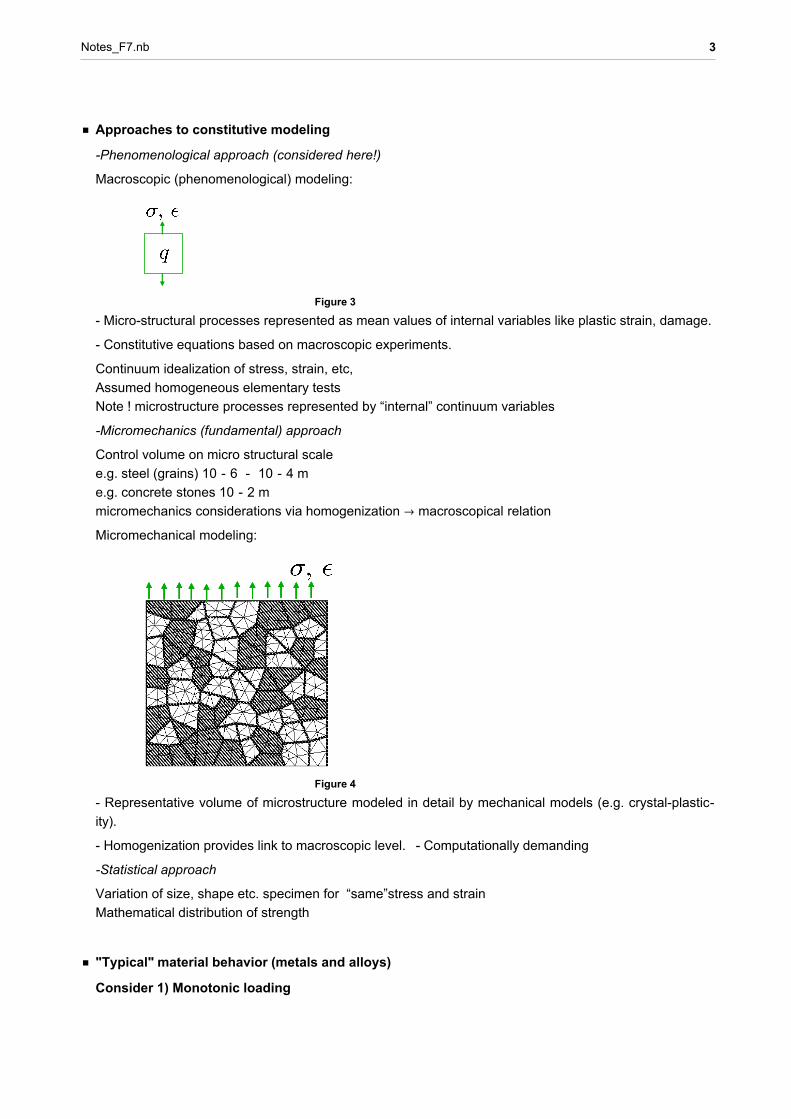
-Micromechanics (fundamental) approach
Control volume on micro structural scalee.g. steel (grains) 10-6 - 10-4 me.g. concrete stones 10-2 mmicromechanics considerations via homogenization Ø macroscopical relation
Micromechanical modeling:
Figure 4
- Representative volume of microstructure modeled in detail by mechanical models (e.g. crystal-plastic-ity).
- Homogenization provides link to macroscopic level.�- Computationally demanding
-Statistical approach
Variation of size, shape etc. specimen for “same”stress and strainMathematical distribution of strength
ü "Typical" material behavior (metals and alloys)
Consider 1) Monotonic loading
Notes_F7.nb 3

Creep and relaxation
- Temperature dependence- Identifiable stages with time fl
Strain rate dependence
- Static (slow) loading- Dynamic (rapid) loading fl “Higher stiffness and strength for larger loading rate”!!
Figure 5
Consider 2) Cyclic loading
Cyclic loading and High--Cycle--Fatigue (HCF)
- Elastic deformation (macroscopically) degradation of elasticity close to failure(Note! “weak” theoretical basis at present)
Cyclic loading and Low--Cycle--Fatigue (LCF)
Consider 1D test:
Figure 6
Response in loading-unloading
4 Notes_F7.nb

Figure 7
Response in loading-unloading-loading-unloading (cyclic behavior)
Figure 8
Test modes: εa = const. or σa = const.
- Plastic deformation in each cycle fl "hysteresis loops"
Isotropic hardening
Figure 9
Kinematic hardening
Notes_F7.nb 5

Figure 10
- Stages of fatigue process, stress control fl
fl Shakedown (=stabilized cyclic curve) or ratcheting behavior
Figure 11
ü Characteristics of material "fluidity"
Creep: ε ≠ 0 when σ = 0
Figure 12
Relaxation: σ ≠ 0 when ε = 0
6 Notes_F7.nb

Figure 13
Stages of creep process (pertinent to stress controlled process):
- Transient (primary) ε decreasing
- Stationary (secondary) ε ∽constant
- Creep failure (tertiary) ε Ø ¶ when t → tR
Figure 14
F7b. Linear viscoelasticity
Duggafrågor1) For a static uniaxial bar problem at isothermal (θ = const. ) conditions, state principle of energyconservation (first law of thermodynamics). On the basis of this relationship, derive the relation e = σ ε ,where e is the internal energy, for the considered bar problem.
Notes_F7.nb 7

2) For the same bar problem as in T3, state the dissipation inequality ≥ 0 . In this context, state theexpression for a stored elastic (or free) energy ψ@ε, κD in the case of the linear visco-elastic Maxwellmodel. Derive also the expression for the uniaxial stress σ and the micro-stress K in the dash-pot. Inaddition, show that the dissipation is positive for the (linear) evolution of the visco-plastic strain.
3) On the basis of the established visco-plastic model derive the model behavior during the step load-ings: Creep behavior: σ@tD = σ0 H@tD and relaxation behavior ε@tD = ε0 H@tD . Assume zero temper-ature change: θ = 0 ⇒ εi = αθ = 0
à Constitutive relations: Introduction to thermodynamic basis
ü Uniaxial bar problem
Assume: 1) Isothermal (θ = const.) process of uniaxial bar!2) Dissipative material: function of strain ∈ (observable) and internal (hidden) variable κ (repr. irreversible processes in microstructure)
Figure 15
ü Consider thermodynamic relations
a) Principle of energy conservation
E + K = W H+QLE = ‡
Le x = Internal energy
K =12 ‡
Lρ u2 x = Kinetic energy = 0 in static case!
W = ‡LU u x + @σ uDx=0
x=L = Mechanical workHQ = Heat supply not consideredLNote! for considered barHσ uL' = σ' u + σ u' = −U u + σ ε ⇒ U u = σ ε − Hσ uL' ⇒
∴ W = ‡LHσ ε − Hσ uL'L x + @σ uDx=0
x=L = ‡Lσ ε x ⇒
Energy equation for static case:
8 Notes_F7.nb

E = W ⇒ ∴ e = σ ε
Note!
e = ‡ε0
ε
σ ε = actual strain energy experienced by material
b) Dissipation (or entropy) inequality
Introduce stored elastic energy: ψ@ε, κD = Helmholtz free elastic energy.Assume strain energy: e = e@εDDef.: Consider dissipation from the inequality
‡L
x = ‡LHe − ψL x ≥ 0 ≥ 0 pointwise
Express entropy inequality; consider dissiplation
:= e − ψ = σ ε −∂ψ∂ε
ε −∂ψ∂κ
κ ≥ 0 ⇒
∴ ≥ 0 σ =∂ψ∂ε
and = K κ ≥ 0 with K = −∂ψ∂κ
ü Dissipative materials - classes
1) Non-dissipative elastic material: =def. 0 fl
ψ = ψ@εD ⇒ = K κ := 0 ⇒ K, κ irrelevant!
e.g. linear thermo-elasticity with
ψ@ε; θD =12 E HεeL2 =
12 E Hε − α θL2 ⇒ σ = E Hε − α θL
2) Viscous dissipative material: ≥ 0 such that K depends on state as
K = f@ε, κ, κDe.g. visco-elasticity or visco-plasticty
ψ@ε; θD =12 E Hε − κ − α θL2 ⇒ σ = E Hε − κ − α θL; K = −
∂ψ∂κ
= σ ⇒
K = σ = µ κ ⇒ =1µ
σ2 ≥ 0 OK!
3) Inviscid (rate-independent) dissipative material: ≥ 0 so that K depends
K = f@ε, κD ε
e.g. elasto-plasticity.
Note! rate-insensitivity; s=another time scale !
ε =dεdt =
dεds
dsdt =
dεds s ⇒ K =
dKds s = f@ε, κD
dεds s ⇒
K = f@ε, κD εdKds = f@ε, κD
dεds
Notes_F7.nb 9

à Prototype model of viscoelastic material - Maxwell model
ü Model definition
Reological model:
Figure 16
Free energy:
ψ@ε, κ; θD =12 E Hε − κ − α θL2 ⇒ σ = K = E Hε − κ − α θL ⇒ K = −
∂ψ∂κ
= σ
Dissipation
= K κ = 9Assume : κ =Kµ, K = σ= =
1µ
σ2 ≥ 0 OK!
fl Evolution of deformation in damper:
κ =1µ
σ, µ > 0 viscosity parameterNote, relaxation time t∗ (used instead of µ ):
t∗ =def. µE ⇒ κ =
1t∗
σE =
1t∗ εe
ü Model behavior for step loading
Assume zero temperature change: θ = 0 ⇒ εi = αθ = 0Creep behavior: σ@tD = σ0 H@tD
Figure 17
Consider evolution rule, t ≥ 0 :
10 Notes_F7.nb

κ =1µ
σ0 , IC : κ@0D = 0Introduce relaxation time: t∗ =def. µ
EEstablish soltution by direct integration as
κ =1µ
σ0 ⇒ κ@tD = C@1D +σ0µ
t = C@1D +σ0E
tt∗
Inititial condition:
κ@0D = 0 ⇒ C@1D = 0Establish solution
σ0 = E Hε − κ@tDL ⇒ ε =σ0 Ht + t∗L
E t∗ = ε0 I tt∗ + 1M
Note! Initially at t = 0 , we get ε@0D = ε0 = σ0E fl Only the spring is activated! (No deformation in
dash-pot)
0.5 1 1.5 2 time t
0.5
1
1.5
2
2.5
3ε@tD×
σ0EStep−loading: creep, increasing t∗
Analysis: Creep behavior: σ@tD = σ0 H@tDRelaxation behavior: strain driven step ε@tD = ε0 H@tD
Figure 18
Consider evolution rule for damper
κ =1µ
σ, t ≥ 0, κ@0D = 0
Notes_F7.nb 11

Establish solution as:
κ@tD =1µ
σ with σ → E Hε0 − κ@tDL ⇒ κ@tD → − tt∗ C@1D + ε0
Establish solution with intitial value κ@0D = 0 and µ → E t∗
κ@tD = H1 − − tt∗ L ε0
σ = E Hε0 − κ@tDL = E ε0 − tt∗
0.5 1 1.5 2 time t
0.2
0.4
0.6
0.8
1
ε@tD×Eε0Step−loading: relaxation, increasing t∗
Analysis: Relaxation behavior: strain driven step ε@tD = ε0 H@tDà Linear (generalized) standard model
Consider generalization in reological model
Figure 19
Free energy:
ψ@ε, κ; θD =12 ‚
α=1
N
Eα Hε − κα − αθL2 ⇒
σ = ‚α=1
N
Eα Hε − κα − αθL = E∞ Hε − αθL − ‚α=1
N
Eα κα with E∞ = ‚α=1
N
Eα
Evolution of deformation in damper:
12 Notes_F7.nb

κα =1µα
Kα, Kα = Eα Hε − κα − αθLDissipation
= ‚α=1
N
Kα κα = ‚α=1
N 1µα
Kα2 ≥ 0 OK!
ü Three parameter model: Linear solid model
Figure 20
Consider special case: α = 2 where
σ = E∞ Hε − αθL − E1 κ1
κ1 = κ =1µ
K, K = E1 Hε − αθ − κL, µ = E1 t∗
κ2 := 0Relaxation behavior fl strain driven step ε@tD = ε0 H@tDwith α θ := 0
κ =1µ
K with K → E1 Hε − κL ⇒ κ@tD = ε0 + − tt∗ C@1D
Initial condition κ@0D = 0 fl
κ@tD = ε0 I1 − − tt∗ M ⇒ σ = E∞ ε0 − E1 κ@tD =. .. = E∞ J 1 + I − t
t∗ − 1M E1E∞
N ε0Note! κ@0D = 0 fl
σ = E¯@tD ε0, E¯@tD = E∞ J 1 + I − tt∗ − 1M E1
E∞N
Note: Maxwell E2 → 0 , E1 = E∞ → E fl E¯@tD = E − tt∗ (cf. previous case)
Notes_F7.nb 13

Figure 21
2000 4000 6000 8000 10000time t
0.2
0.4
0.6
0.8
1
σ@tD×E∞ε0Relaxation: 3−parameter
ü Summary: Linear elasticity
Consider σ = E¯@tD ε0 as linear relation at given times t fl Isochrones
Figure 22
0.2 0.4 0.6 0.8 1ε0E∞
0.2
0.4
0.6
0.8
1σ@tD Isocrones : Solid behavior
Figure 23
0.2 0.4 0.6 0.8 1ε0E∞
0.2
0.4
0.6
0.8
1σ@tDIsocrones : Fluid behavior HMaxwellL
Remove@"`∗"D
14 Notes_F7.nb