f. - NASA · OF TIME AT CAPE KENNEDY, FLORIDA by Jltnzes R. Scoggim, M. M. Perzdepst, arid V, E....

f.

v- -#

N A S A C

R

AN INVESTIGATION OF SMALL-SCALE MOTIONS A N D THE FORECASTING OF W I N D PROFILES OVER SHORT PERIODS OF TIME AT CAPE KENNEDY, FLORIDA

by Jltnzes R. Scoggim, M . M . Perzdeps t , arid V, E.

Prepn red by TE-XAS A & M UNIVERSITY Cdlege Station, Texas

foz George C. Marshall Space Flight Center \ .' \-+.L:L-+ €:a i

N A T I O N A L A E R O N A U T I C S A N D S P A C E A D M I N I S T R A T I O N WASHINGTON, D. C. A P R I L 1970

https://ntrs.nasa.gov/search.jsp?R=19700014618 2018-10-06T07:07:31+00:00Z

TECH LIBRARY KAFB, NM

I . REPORT NO. & W O . 2. GOVERNMENT ACCESSION NO. 3. RECIPIENT'S CATALOG NO.

/NASA CR-1534 0. F L E AND S U B T I T L E

k# INVESTIGATION OF SMALL-SCALE MOTIONS AND THE FORECASTING * r S W O 5. REPORT DATE

IF WTM> PROFEES OVERS SHORT PERIODS O F TIME AT CAPE REmEDY, 6. PERFORMING ORGANIZATION CCoE

FLORIDA tL&LJR:-r: r*cuLp-d& . . - 3 " a _ . . 7. AUTHOR(S] d 8-PERFORMING ORGANIZATION REPORr R

James R. Scoggins, M. M. Pengrgas t , and. V. E. Moyer 3. PERFORMING ORGANIZATION NAME AND ADDRESS 1 0 . WORK UNIT NO.

dexas A & M Univ" -=4c=a 1 1 . CONTRACT OR GRANT NO,

NAS8-21257 &.u" 13. TYPE OF REPOR-; PERIOD COVEREC

2. SPONSORING AGENCY NAME AN0 ADDRESS Contractor Report NASA-George C. Marshall Space Flight Center Marshall Space Flight Center, Alabama 35812 1 4 . SPONSORING AGENCY CODE

I

15. SUPPLEMENTARY NOTES This work was performed for the .Aerospace Environment Division ot the Aero-Astrodynamics Laboratory, MSFC, with M r . William W. Vaughan as Contract Monitor.

hd5-i c ! + + B , ~ A - , c $ 16. ABSTRACT

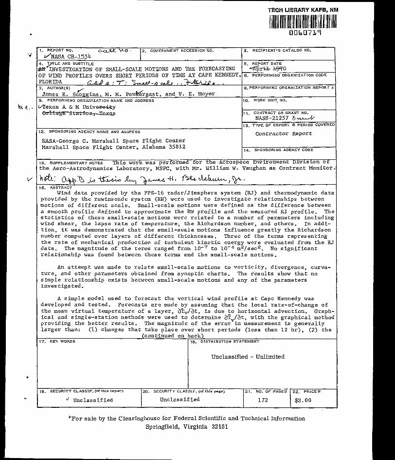
Wind data provided by the FPS-16 radar/Jimsphere system (RJ) and thermodynamic data provided by the rawinsonde system (RW) were used to inves t iga te re la t ionships between motions of different scale. Small-scale motions were defined as the difference between a smooth profile defined to approximate the RW p r o f i l e and the measured RJ prof i le . The statistics of these small-scale motions were re la ted to a number of parameters including wind shear , the lapse rate of temperature, the Richardson number, and others. In addi- t ion , i t was demonstrated that the small-scale motions influence greatly the Richardson number computed over layers of different thicknesses. Three of the terms represent ing the rate of mechanical production of turbulent kinetic energy were evaluated from the R J data. The magnitude of the terms ranged from t o 10" m2/sec2. No s ign i f i can t re la t ionship was found between these terms and the small-scale motions.

An attempt was made to relate small-scale motions to vorticity, divergence, curva- tu re , and other parameters obtained from synoptic charts. The r e su l t s show tha t no s imple re la t ionship exis ts between small-scale motions and any of the parameters invest igated.

A simple model used to fo recas t t he ve r t i ca l wind p r o f i l e a t Cape Kennedy was developed and tested. Forecasts are made by assuming that the local rate-of-change of the mean virtual temperature of a layer , aTv/at, is due 50 horizontal advection. Graph- i c a l and s ingle-s ta t ion methods were used to determine aTv/at, with the graphical method providing the bet ter resul ts . The magnitude of the e r ror in measurement is general ly l a rge r than: (1) changes that take place over short periods (less than 1 2 h r ) , (2) t he

(continued on back) 17. KEY WORDS 18. DISTRIBUTION STATEMENT

Unclassified - Unlimited

19. S E C U R I T Y C L A S S I F . p f this r e p a t ) 20. SECURITY CLAI:SIF. (of t h i s 21. NO. OF PAGE^' 22. PRICES

Unclassified Unclassified 172 $3.00

*For sale by the Clearinghouse for Federal Scientific and Technical Information Spr ingf ie ld , Vi rg in ia 32 151

magnitude of ageostrophic motions, and (3) the magnLtude of the e r ror expected because of vertical motion. It was found tha t t he model is no bet ter than pers is tence for per iods less than 9 hours. It does seem t h a t for per iods greater than 9 hours, the model could be useful.

c

Y

.

FOREWORD

This report i s composed of nine sect ions and two appendices.

The f i r s t seven sect ions deal wi th the s ta t is t ical p rope r t i e s of

t he small-scale or turbulent motions and relationships between these

motions and synoptic-scale parameters. Section V I 1 1 deals with the

problem of forecasting the wind profile over short periods of t i m e

a t Cape Kennedy from synoptic-scale data. It i s essent ia l ly inde-

pendent of Sections I - V I I , thus making i t poss ib le for the reader

to omit Sect ion V I 1 1 i f desired. Appendix B i s a Master's Thesis

prepared by Captain James H. Blackburn, Jr. Capt. Blackburn used

data provided by NASA i n t he p repa ra t ion of h i s t h e s i s . The research

conducted by Capt. Blackburn i s essent ia l ly independent o f , although

somewhat r e l a t ed t o , t he r e sea rch r epor t ed i n t h i s r epor t . H i s t hes i s

may be read independently of the remainder of the repor t a l though in

many respec ts i t complements the research reported i n Sections I - V I I .

iii

A

ACKNOWLEDGMENTS 7

The authors are indebted to a number of people who provided

a s s i s t a n c e i n t h e r e s e a r c h as w e l l a s the p repara t ion of th i s re-

por t . We apprec ia te s incere ly the work performed by Capt. Robert

Croft in preparat ion of computer programs. We are indebted t o t h e

NASA Contract Monitor, Mr. William W. Vaughan, who made many sug-

gest ions and comments regarding the research while i t was i n progress;

t o M r . Robert Henderson, Mrs. Carmelita Budge, and Miss Joyce Dal-

rymple fo r t he i r suppor t and u n t i r i n g e f f o r t s i n t h e a n a l y s i s of data,

and in t he p repa ra t ion o f t he f i na l r epor t , and ; t o Drs. W.S. McCully

and K.C. Brundidge f o r t h e i r a s s i s t a n c e i n t h e p r e p a r a t i o n o f

Section VIII.

r

.

Sect ion

TABLE OF CONTENTS

T i t l e

FOREWORD

ACKNOWLEDGMENTS

TABLE OF CONTENTS

LIST OF FIGURES

LIST OF TABLES

I. INTRUDUCTION

11. DATA

A. Source and E x t e n t

B. M a t c h i n g of RW and R J Prof i les

C. Prepara t ion of D a t a €or M a c h i n e Processing

111. DATA PROCESSING

A. C o m p u t a t i o n s Performed at Texas A&M

€3. C o m p u t a t i o n s P e r f o r m e d a t MSFC

I V . D E F I N I T I O N O F SMALL-SCALE MOTIONS

A.. S m o o t h i n g of Wind Profiles

B. S m o o t h i n g of Slant R a n g e

C. Relationships B e t w e e n S m a l l - S c a l e M o t i o n s D e f i n e d by the D i f f e r e n t M e t h o d s

V. THEORETICAL CONSIDERATIONS

A. The Energy Equation

B. The Richardson N u m b e r

V I . EVALUATION OF STRESS/SHEAR TENSOR I N TRE ENERGY EQUATION

Page

iii

iv

V

vii

X

1

8

8

10

10

12

12 13

16

V I 1 . RELATIONSHIPS BETWEEN SMALL- SCALE MOTIONS ASSOCIATED W I T H DETAILED WIND PROFILES AND SELECTED EETEOROLOGICAL PARAMETERS 22

V

Section Title

A,. Lapse Rate of Temperature

B. Vertical Wind Shear C. The Richardson Number D. Parameters Determined from Synoptic Charts

VIII. A SIMPLE METHOD FOR FORECASTING THE WIND PROFILE A. Introduction and Background of Problem B. Wind Measurement and Data

C. The Forecast Model

D. Discussion of Factors Related to the Forecast Model 1. Location of Data

2 . Forecasting Plean Virtual Temperature (FV)

3 . Vertical Motion 4. Ageostrophic Motion

or Thickness (Ah)

E. Use of the Model

IX. SUMMARY

REFERENCES

APPENDIX A

APPENDIX B

.. Page

22

24

24

41

56

56

6 2

64

9

68

68

70

78

83

87

94

98

A- 1

B- i

vi

Figure

LIST OF FIGURES

T i t l e Page

.

1.

2.

3.

4 .

5 .

6 .

7 .

8 .

9.

An example of smoothing of a measured p ro f i l e . Turbulent motions are defined as the d i f f e rence between the smooth and measured p r o f i l e s

Magnitude of t h e rate of mechanical production of tu rbulen t k ine t ic energy vs the magnitude of turbulent kinet ic energy, U ' V '

Magnitude of t h e rate of mechanical production of tu rbulen t k ine t ic energy vs the magnitude of turbulent kinet ic energy, U ' W '

Magnitude of the rate o f mechanical production of turbulent kinet ic energy vs the magnitude of turbulent kinet ic energy, v ' w '

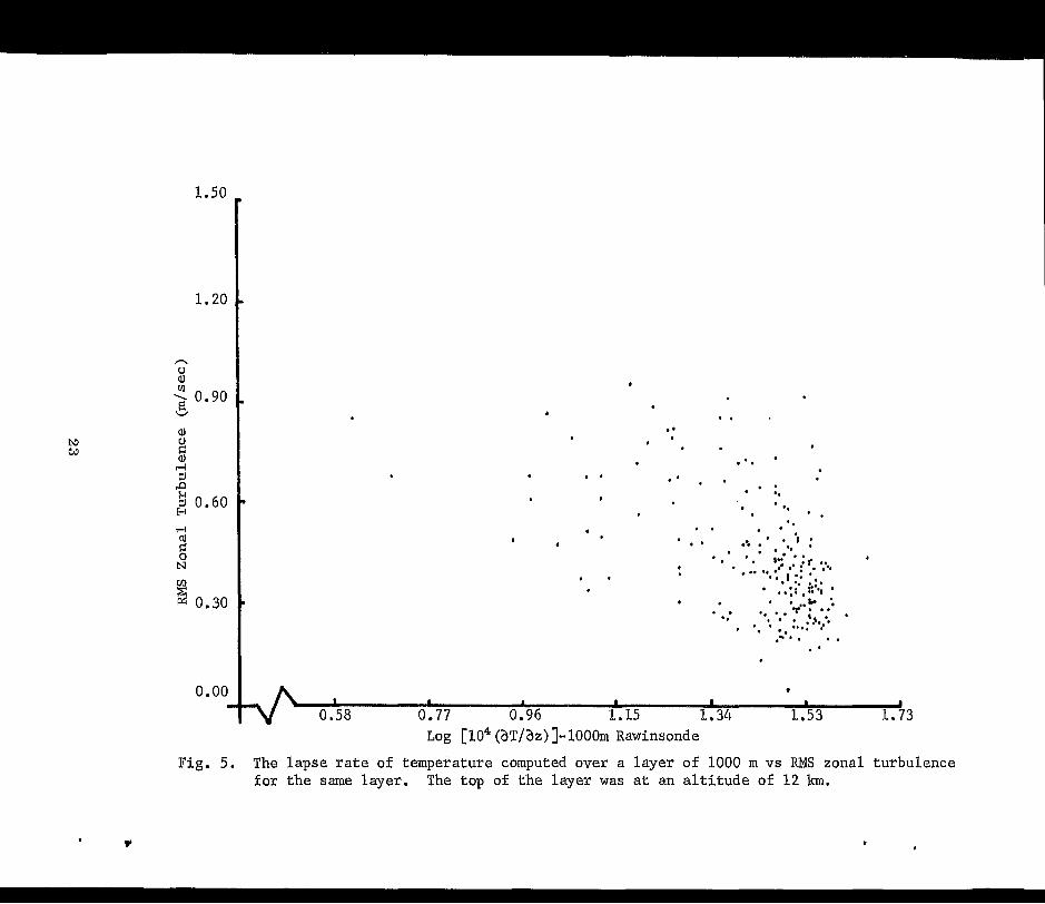
The lapse rate of temperature computed over a layer of LOO0 m vs RMS zonal tu rbulence for the same layer . The top of the layer w a s a t an a l t i t u d e o f 12 km

The vector vertical wind shear computed over a layer of 1000 m vs RMS zonal turbulence for the same layer . The top of t he l aye r w a s a t an a l t i t u d e o f 1 2 km

T h e Richardson number computed over a l aye r of 1000 m vs t h e RMS of the zonal tu rbulence for the same layer . The top of t h e l a y e r was a t an a l t i t u d e of 1 2 km. W winds and RW temperatures w e r e used i n t h e computations

The Richardson number computed over a layer of 500 m with R J winds vs the Richardson number computed over the same layer wi th RW winds. The top of the layer w a s a t a n a l t i t u d e of 1 2 km

The Richardson number computed from R J winds and RW temperatures vs the Richardson number computed from RW winds and temperatures. The computations w e r e performed over a layer of 1000 m wi th the top of the l aye r a t 1 2 km

9

19

20

21

23

25

30

37

38

vii

Figure

10.

11.

12.

13.

14.

15.

16.

17.

18.

19.

20.

Title

The Richardson number computed over a layer of 500 m vs the Richardson number computed over a layer of 2000 m. The top of each layer was at an altitude of 12 km. RJ winds and RW temperatures were used in the computations

The vector vertical wind shear computed over an altitude interval of 500 m vs wind shear over an altitude interval of 2000 m. RJ data were used in the computation and the top of each layer was at an altitude of 1 2 km

Synoptic naps for Case 1, April 5, 1966

Temporal cross sections of changes in wind speed (m/sec) (A,, B, and C) and RMS of small-scale motions (hundreths of m/sec) (D, E, and F) computed over 1 km for Case 1, April 5, 1966

Synoptic maps for Case 2, April 8 , 1966-

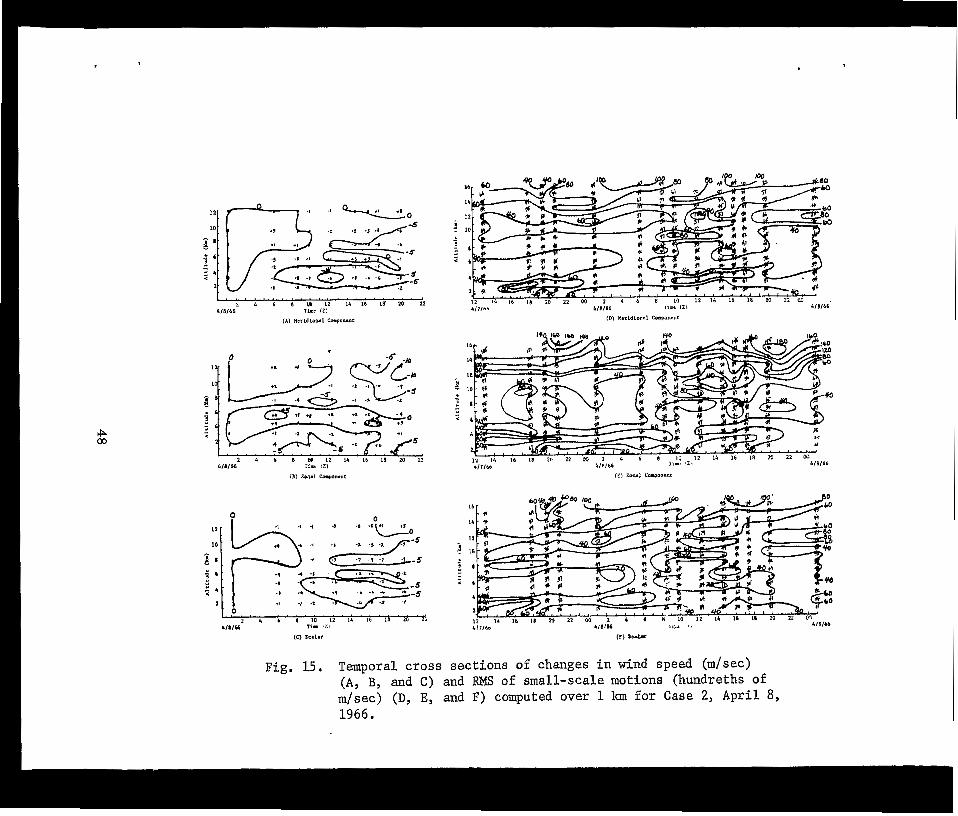
Temporal cross sections of changes i n wind speed (m/sec) (A, B, and D) and RMS of small-scale motions (hundreths of m/sec)(D, E, and F) computed over 1 km for Case 2, April. 8 , 1966

Synoptic maps for Case 3 , July 5, 1966

Temporal cross sections of changes in wind speed (m/sec)’(A, €5, and C) and RMS of small-scale motions (hundreths of m/sec) (D, E, and P) computed over 1 km for Case 3 , July 5, 1966

Synoptic maps for Case 4, September 11, 1966

Temporal cross sections of changes in wind speed (m/sec) (A, B, and C) and RMS of small-scale motions (hundreths of m/sec) (D, E, and F) computed over 1 km for Case 4 . , September 16, 1966

A map of rawinsonde stations in the Cape Kennedy area (circles) and locations of stations forming the desired 4-point grid (plus signs)

Page

39

40

43

44

46

48

50

5 1

5 2

53

69

viii

Figure T i t l e Page

21.

22.

23.

24.

ix

73

A comparison of the forecast change of thickness f o r t h e 700-500-mb and the 500-300-mb layer over a 12-hr period, and t h e measured change of thickness a t Jacksonvi l le , Miami, and Cape Kennedy. Points fa l l ing within the dashed l ines represent within measurable accuracy (2 28 m) an acceptable fo recas t

A comparison of the fo recas t and measured change in t he g rad ien t o f t h i ckness between Jacksonville and Miami over a 12-hr period for the 700-500-mb and 500-300-mb l aye r s . Po in t s f a l l i ng w i th in t he dashed lines represent within measurable accuracy (* 40 m) an acceptable forecast 76

Comparison of t he Rpls e r r o r i n wind fo recas t s by the advection of mean v i r tua l t empera ture o r th ickness wi th pers i s tence and climatology a t Cape Kennedy 89

Relative location of rawinsonde stations used t o compute wind fo recas t s fo r Oklahoma City 92

L

LIST OF TABLES w

Table T i t l e

1. Correlation coefficients between RMS values of small-scale motions defined by d i f f e r e n t methods

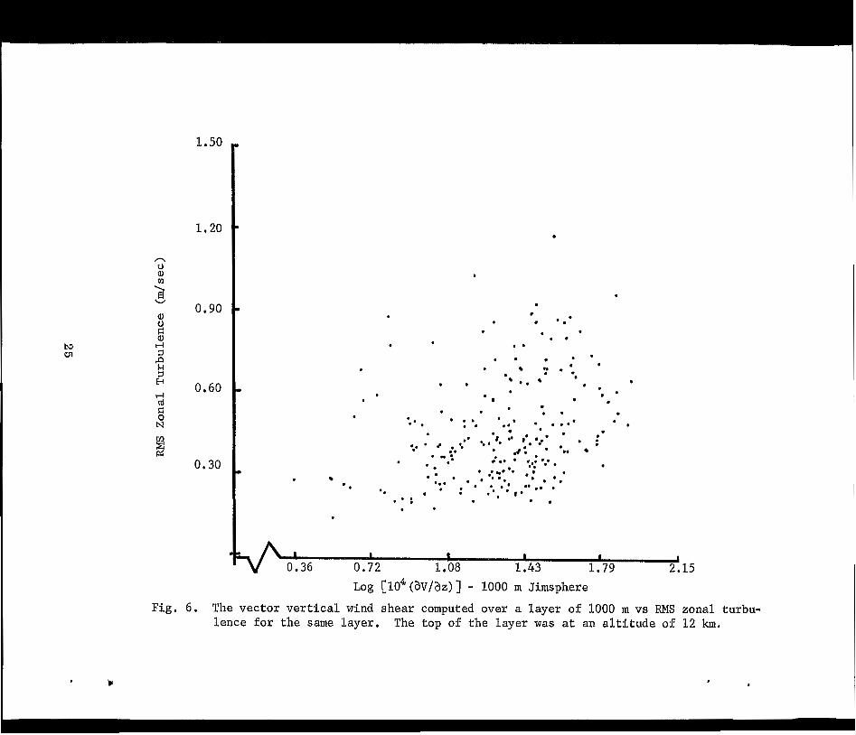
2. Empirical correlations between R i and CAT (taken from Reiter and Lester, 1967)

3. The relative frequency of balloon-measured turbulence versus Richardson number wi th the top of the l ayer a t 6 km. Computations were performed over a layer of 1000 m. Tota l number of da ta po in ts - 240

4 . The relat ive f requency of balloon-measured turbulence versus Richardson number with the top of t he l aye r a t 1 2 km. Computations were performed over a layer of 1000 m. Total number of data points - 225

5. The relat ive f requency of balloon-measured turbulence versus Richardson number wi th the top of the l ayer a t 16 km. Computations were performed over a layer of 1000 m. Tota l number of data points - 195

6. A est imate of the magnitude and d i rec t ion of v e r t i c a l motion based on the sign of i soba r i c advection of temperature and v o r t i c i t y

7. Relat ive magni tude of the effect of ver t ical motion a t Miami and Jacksonvi l le on the zonal wind speed a t Cape Kennedy

8. The RMS e r r o r s of fo recas t s of zonal wind speed a t Cape Kennedy categorized according to the ind ica to r s o f vert ical motion

Page

11

26

31

32

33

79

82

83

9. The RMS of t he d i f f e rence between the zonal wind computed from the geostrophic wind equation, and that obtained from R J d a t a a t Cape Kennedy, F lor ida 84

10. Comparison of t h e RMS er ror o f forecas ts usFng the s ing le - s t a t ion method and t h e RMS e r ror o f persistence for a period of 6 h r a t Oklahoma C i t y . The number of cases i s 65 91

X

I

I. INTRODUCTION

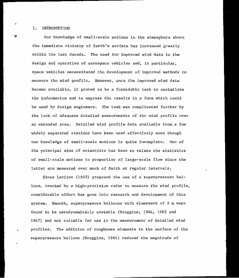
3 Our knowledge of small-scale motions i n t h e atmosphere above

the immediate vicini ty of Earth's sur face has increased grea t ly

wi th in the last decade. The need f o r improved wind d a t a i n t h e

design and operat ion of aerospace vehicles and, in par t icular ,

space vehicles necessitated the development of improved methods t o

measure the wind p ro f i l e . However, once the improved wind d a t a

became ava i lab le , i t proved t o b e a formidable task to assimilate

the information and t o e x p r e s s t h e r e s u l t s i n a form which could

be used by design engineers. The task was complicated further by

the lack of adequate detailed measurements of the wind p ro f i l e ove r

an extended area. Detailed wind p r o f i l e d a t a a v a i l a b l e from a f e w

widely separated stations have been used effectively even though

our knowledge of small-scale motions i s quite incomplete. One of

t he p r inc ipa l a i m s o f s c i en t i s t s has been t o relate t h e statist ics

of small-scale motions to p rope r t i e s of large-scale f low s ince the

lat ter are measured over much of Earth a t r egu la r i n t e rva l s .

Since Leviton (1962) proposed the use of a superpressure bal-

loon, tracked by a high-precis ion radar tb measure the wind p r o f i l e ,

cons ide rab le e f fo r t has gone in to r e sea rch and development of t h i s

system. Smooth, superpressure bal loons with diameters of 2 m w e r e

found t o be aerodynamically unstable (Scoggins, 1964, 1965 and

1967) and n o t s u i t a b l e f o r u s e i n t h e measurement: of d e t a i l e d wind

p ro f i l e s . The addition of roughness elements to the surface of t h e

superpressure balloon (Scoggins, 1964) reduced the magnitude of

- these aerodynamically-induced oscillations, and thereby provided a

spherical balloon which w a s aerodynamically stable. This balloon

configuration, now known as the "Jimsphere," has since been deter-

mined t o b e a s u i t a b l e wind sensor for most purposes (Eckstrom,

1965; Za r t a r i an and Thompson, 1968; Scoggins, 1967).

P

It has been shown (Eckstrom, 2. G.) that the response of the

Jimsphere i s adequate to measure wind shears over an a l t i tude in te r -

val of a few meters, and also that the remaining self-induced

motions are f i l t e r e d o u t by t h e data reduction program (Rogers and

Camnitz, 1965). Thus t h e RMS errors of approximately 0.6 m/sec

and less found by Scoggins (1967) and Susko and Vaughan (1968) were

due p r imar i ly t o e r ro r s i n r ada r da t a . A discussion of e r r o r s i n

t h e FPS-16 radar and the i r in f luence on the measurement of wind d a t a

i s presented i n a paper by Scoggins and Armendariz (1969). The

a l t i t u d e r e s o l u t i o n of t h e wind d a t a i s believed to be approximately

50 m although this s t i l l i s an unsett led question because of uncer-

t a i n t i e s i n spec i fy ing radar e r ror , ed i t ing the r a w radar data , and

processing the data . However, t h e wind p ro f i l e da t a ob ta ined by

t h i s method i s at least one order of magnitude more accurate than

those provided by the rawinsonde (RW)* system.

Sawyer (1961) performed a study of mesoscale motions associated

w i t h v e r t i c a l wind p r o f i l e s . From ba l loon da ta wi th a r e so lu t ion

Q RW and RJ w i l l be used for rawinsonde and FPS-16 radar/Jim- sphere, respectively.

2

- P considerably poorer than that provided by t h e FPS-16 radar/Jimsphere

(RJ) system, he observed features which w e r e p e r s i s t e n t and main-

ta ined the i r ident i ty over per iods o f severa l hours . Similar and

even smaller features have been observed on the detai led prof i les

provided by t h e R J system (Weinstein e t al., 1966; DeMandel and

Scoggins, 1967; and o the r s ) . While a sa t i s fac tory theory has no t

been developed to explain a l l of the observed features, some exh ib i t

the p roper t ies o f wave mot ions charac te r i s t ic o f iner t ia , shear -

grav i ty , g rav i ty , and other types of waves. Some of the h igh f re -

quency components whose character changes from observation to ob-

servat ion apparent ly are due t o turbulent motions.

The improved wind prof i le data have been used i n a number of

s t u d i e s r e l a t i n g t o t h e d e s i g n and operat ion of aerospace vehicles

(see, f o r example, Ryan e t al., 1967; Blackburn, 1968). Many of

these s tud ies dea l t wi th the in f luence o f smal l - sca le mot ions on

the vehic le , s ince they are important i n terms of the i r cont r ibu-

t i o n t o v e h i c l e r e s p o n s e and loads caused by t h e wind. Scoggins

and Vaughan (1964) discussed general aspects of the importance of

atmospheric motions of different scale i n t h e d e s i g n of space vehi-

cles. Vaughan (1968) described the use of the R J system i n moni-

t o r ing wind condi t ions p r ior to the launch of space vehic les a t

Cape Kennedy.

I n most s tud ie s r e l a t ing t o t he des ign and operation of aero- R

space vehicles, assumptions must be made regard ing the re la t ion-

ships between motions of different scale. The b a s i c d e s i g n c r i t e r i a -

3

,.

developed for the Saturn vehicle (Daniels, et al., 1966) employs a

number of assumptions regarding the relationships between quasi-

steady-state wind speed, wind shears over various intervals of alti-

tude, and gusts. The total response of the vehicle in terms of

control system requirements as well as structural loading is a

function of these relationships. For this reason this subject has

received considerable attention during recent years.

The primary purposes of this research were to investigate the

relationships between motions of different scale by use of data

provided by the RW and RJ systems, and to ascertain to what extent

the wind profile can be forecast over short periods of time at

Cape Kennedy. The results of this research are reported in the

following sections of this report.

9 11. DATA

A. Source and Extent

Wind p r o f i l e d a t a f r o g t h e RW and Rs systems were provided by

the Aerospace Environment Division, NASA Marshall-Space Flight

Center. The RW d a t a w e r e i n a form of computer output while the RJ

d a t a were on magnetic t a p e and microfilm. The period covered by

t h e d a t a w a s 1965 t o 1968; however, d a t a w e r e no t ava i l ab le fo r

each day and i n some cases no d a t a w e r e a v a i l a b l e f o r a number of

successive days.

The RW data consisting of pressure, temperature, humidity, and

wind d i r e c t i o n and speed were presented a t 250-m i n t e r v a l s from near

t he su r f ace t o t he lower s t ra tosphere . The R J data were presented

a t i n t e r v a l s o f 25 m f rom near the sur face to an a l t i tude of ap-

proximately 18 km, although some of these p rof i les t e rmina ted a t a

somewhat lower a l t i t u d e .

B. Matching of RW and RJ P r o f i l e s

Most of the RW runs w e r e made a t 00 o r 12Z on a r egu la r bas i s

and w e r e ava i lab le for each day. These data appear to be remarkably

cons is ten t wi th very f e w quest ionable points . A l s o a very small

percentage of these data were missing. The d e t a i l e d wind p r o f i l e

d a t a were no t measured on a s t r ic t schedule , a l though many of t h e

data corresponded to the 00 and 122 RW da ta . In addi t ion , there

w e r e a number o f p ro f i l e measurements made a t times between the .

RW p r o f i l e s as w e l l as approximately 20 sets of serial ascents

5

containing between 8 and 15 p r o f i l e measurements. I n t h e s e series Ft

of p rof i les there w a s a t i m e i n t e r v a l o f approximately 1 t o 2 hours

between successive profiles with one or more RW measurements made

during each series. Since thermodynamic d a t a must be obtained from

t h e RW runs fo r u se w i th t he de t a i l ed wind p r o f i l e s , measurements

made by t h e t:wo systems had t o b e matched. I f t h e t i m e i n t e r v a l

between the RW wind p r o f i l e and the R J wind p r o f i l e w a s 2 hours or

Less, they were considered to be a matched pair . There were ap-

proximately 300 matched pa i r s i n t he da t a , bu t because o f missing

p o i n t s i n e i t h e r t h e RW o r R J data, about 50 of the sets were not

used i n t h e a n a l y s i s . The remaining 250 sets of p r o f i l e s were

near ly complete over the a l t i tude of i n t e r e s t and were determined

to be reasonable by a v isua l inspec t ion .

C. Preparation of Data f o r Machine Processing

The RW data for the approximately 250 p r o f i l e s were key-

punched to permit machine processing. Data f o r each sounding

included altitude, pressure, temperature, humidity, wind d i r e c t i o n

and speed, and d a t e and t i m e . It w a s not necessary to key-punch

any of the R J wind p ro f i l e da t a s ince t hese were provided by NASA

on magnetic tape.

111. DATA PROCESSING

A. Computations Performed a t Texas A.&M

Computer programs were prepared at Texas ASLM t o d e f i n e small-

scale motions from the RJ wind p ro f i l e s , and t o compute the l apse

rate i n temperature, vertical wind shear, the Richardson number,

t h e Colson-Panofsky CAT. index, the statist ical propert ies of s m a l l -

scale motions, and numerous statist ical parameters descr ib ing the

charac te r i s t ics o f the smal l - sca le mot ions . In addi t ion , a special

program w a s requi red for the p repara t ion of a magnetic t a p e con-

t a in ing t he RW da ta .

B. Computations Performed a t MSFC

The or ig ina l radar da ta ob ta ined a t 0.1-sec intervals w e r e

processed a t t h e MSFC Computation Laboratory t o d e f i n e small-scale

motions as represented by var ia t ions in s lan t range . These compu-

t a t i o n s w e r e provided by MSFC s ince a computer program w a s i n

existence for performing the computations, and a l so s ince i t w a s

no t f ea s ib l e to provide the l a rge number of magnetic tapes required

to t r ansmi t t he da t a to Texas A&M. The r e s u l t s w e r e provided i n

the form of tabulated output as w e l l as i n g r a p h i c a l form. These

computations w e r e used in conjunction with those performed a t Texas

ASLM t o arrive a t a s u i t a b l e d e f i n i t i o n of small-scale motions (see

Sect ion IV) .

7

- I V . DEFINITION OF SMALL-SCALE MOTIONS 9

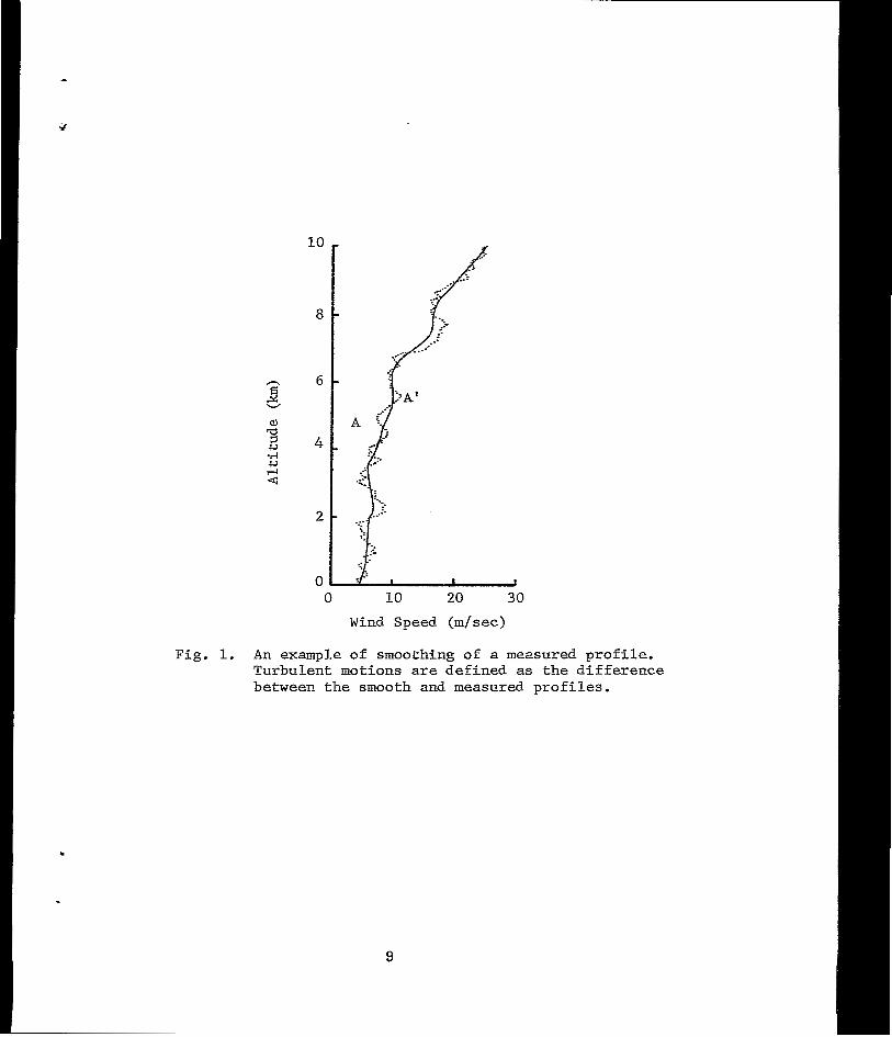
A. Smoothing of Wind P r o f i l e s

The R J wind p ro f i l e s con ta in much more de t a i l than those

provided by the RW method. The d e t a i l e d wind p ro f i l e s con ta in

wave lengths of approximately 100 m and longer and represent vari-

a t ions i n t he ho r i zon ta l wind f i e l d as a function of a l t i t u d e .

Small-scale motions were defined by use of a f i l t e r f u n c t i o n which,

when a p p l i e d t o t h e measured wind p ro f i l e , de f ines a smooth o r

average wind p r o f i l e which varies as a func t ion of a l t i tude . An

i l l u s t r a t i o n i s given i n Fig. 1. The smoothing weights and t h e

associated t ransfer funct ion are given by Scoggins (1967). This

f i l t e r func t ion p rov ides a smooth p ro f i l e con ta in ing wave lengths

of approximately 1000 m and longer. Thus the p ro f i l e o f t he d i f -

ferences between the smooth p r o f i l e and t h e measured p r o f i l e con-

tain wavelengths of approximately 1000 m and less. I n t h i s s t u d y

small-scale motion has been defined as the d i f f e rence between t h e

smoothed and measured wind p ro f i l e s . It i s apparent tha t the

propert ies of small-scale motions defined i n t h i s manner are a

funct ion of the data processing methods employed. For th i s r ea son

i t was deemed d e s i r a b l e t o d e f i n e t h e small-scale motions by a

second method and t b compare t h e r e s u l t s . This second method w i l l

now be discussed.

..

A

0 10 20 30

Wind Speed (m/sec)

Fig. 1. An example of smoothing of a measured p r o f i l e . Turbulent motions are defined as t he d i f f e rence between t h e smooth and measured p ro f i l e s .

9

B. Smoothing of S lan t Range P

From the procedure developed by Endlich and Davies (1967),

measurements of the s lan t range w e r e averaged over a 1-min period;

deviat ions from t h i s mean were used to represent small -scale motions.

Slant range was chosen as t he va r i ab le t o be smoothed because of

i t s accuracy and also because i t would be the best indicator of

small-scale motions of the balloon. From these data the magnitude

of the small-scale motions along the radar beam can be determined;

these would approximate c losely the horizontal component when the

elevat ion angle i s r e l a t i v e l y small. It seems a p p a r e n t t h a t i f

the data-reduction method employed t o compute the wind p r o f i l e s

smoothed so much that the small-scale motions were not adequately

represented, the small-scale motions defined by smoothing the wind

p r o f i l e s and by smoothing the slant-,range data would not show the

same propert ies . Since i t would be much more convenient to work

with the wind. prof i le data than with the s lant-range data , re la-

t ionships between small-scale data defined by the two methods were

invest igated.

C. Relationships Between Small-scale Motions Defined by t h e Different Methods

The RMS of the turbulent f luctuations (small-scale motions)*

w a s determined over layers of 250, 500, 1000, 2000, and 5000 rn for

I

Jc In this report "small-scale motions" and "turbulence" are used interchangeably. They are not necessar i ly synonymous but no d i s t i n c t i o n is made here.

10

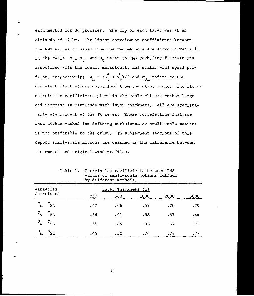
. each method f o r 8 4 pro f i l e s . The top of each layer was a t an

a l t i t u d e o f 1 2 km. The l inea r co r re l a t ion coe f f i c i en t s between ' 2

t h e RMS values obtained from t h e two methods a r e shown i n T a b l e 1.

I n t h e t a b l e cU, 0 and 0 r e f e r t o RMS tu rbu len t f l uc tua t ions V' v

associated with the zonal, meridional, and scalar wind speed pro-

f i l e s , r e s p e c t i v e l y ; 0 = (0 + ov)/2 and osL r e f e r s t o RMS

turbulent f luctuat ions determined from the s l an t r ange . The l i n e a r

co r re l a t ion coe f f i c i en t s g iven i n t he t ab l e all a r e r a t h e r l a r g e

and increase in magni tude with layer thickness . A l l a r e s t a t i s t i -

c a l l y s i g n i f i c a n t a t t h e 1% level. These cor re la t ions ind ica te

t h a t e i t h e r method for def in ing tu rbulence o r small-scale motions

is no t p re fe rab le t o t he o the r . I n subsequen t s ec t ions o f this

report small -scale motions are def ined as the difference between

t h e smooth and o r i g i n a l wind p ro f i l e s .

2 2

H U

Table 1. Correlat ion coeff ic ients between RMS values of small-scale motions defined by d i f f e r e n t methods.

Variables Layer Thickness (m) Correlated 25 0 5 00 1000 200 0 5000

0 0 u SL .47 .66 - 6 7 (. 70 .79

0 0 v SL .36 .44 .68 .67 .64

Q C T v SL .54 .65 .83 .67 .75

0 0 H SL .45 .50 .74 .74 .77

4

V. THEORETICAL CONSIDERATIONS

A. The Energy Equation

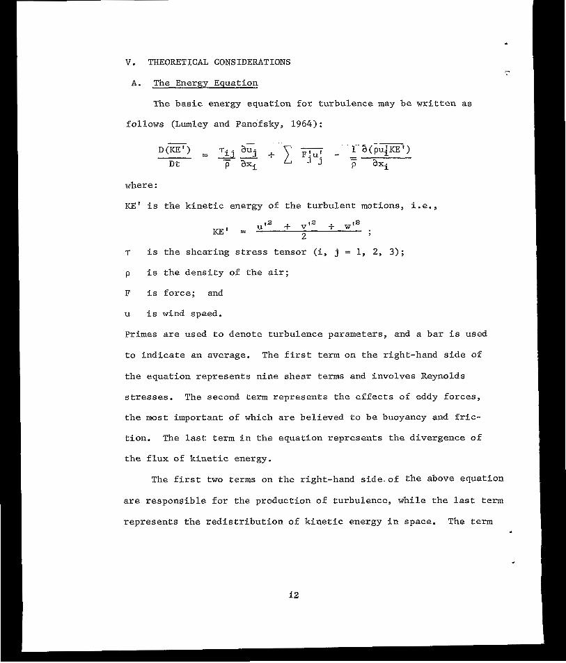
The basic energy equation for turbulence may be wr i t t en as

follows (Lumley and Panofsky, 1964):

where :

KE' i s the kinetic energy of the turbulent motions, i . e . ,

T i s the shear ing stress tensor (i, j = 1, 2, 3 ) ;

p i s the dens i ty o f the a i r ;

F i s force ; and

u i s wind speed.

P r i m e s are used to denote turbulence parameters, and a bar i s used

to indicate an average. The f i r s t t e r m on the r ight-hand side of

the equat ion represents nine shear terms and involves Reynolds

stresses. The second term represents the effects of eddy forces,

t he most important of which are bel ieved to be buoyancy and f r i c -

t ion . The l a s t t e r m i n the equation represents the divergence of

the f lux o f k ine t ic energy .

The f i r s t two terms on the r ight-hand side.of the above equation

are responsible for the production of turbulence, while the last term

represents the red is t r ibu t ion of k ine t ic energy in space . The term

12

involving shearing stresses and wind shears o f ten i s reduced t o

only one term involving stress along the mean wind and the v e r t i c a l

wind shear. The r eason fo r t h i s s imp l i f i ca t ion seems t o be t h a t

measurements near Earth's surface, where the frictional influence

i s grea t , show t h a t a l l o the r components of the shear ing stress

and wind shear are small i n comparison t o t h a t i n t h e downwind

d i r e c t i o n . I n a d d i t i o n , s u i t a b l e d a t a u s u a l l y are not ava i lab le

to permit evaluat ion of a l l t h e terms even i f they are important,

and invest igators tend to fol low precedent . In the f ree a tmosphere

away from the i n f luence of s u r f a c e f r i c t i o n , less i s known about

the magnitudes of the various terms i n t h e stress tensor, al though

a reasonable knowledge about t h e wind s h e a r s i n a l l t h r e e s p a t i a l

d i r e c t i o n s exists. For tuna te ly the wind p ro f i l e da t a p rov ided by

t h e RJ system can be used t o i n v e s t i g a t e the magnitude of several

terms.

B. The Richardson Number

A n investigation of the magnitude of the terms i n t h e energy

equation when app l i ed nea r Ea r th ' s su r f ace i nd ica t e t ha t , i n t he

shear t e r m , o n l y t h e v e r t i c a l wind shear i s of importance, and,

i n t h e eddy force term, only the buoyancy i s of importance. Richard-

son (see Sutton, 1953) defined a nondimensional number, which is

widely known as the Richardson number, as t h e r a t i o of buoyancy t o

wind shear . H e r a t i o n a l i z e d t h a t i n a laminar flow w h e r e turbu-

len t k ine t ic energy d id no t ex is t tu rbulence would begin when t h i s

13

nondimensional number became less than unity. Thus a limiting

value o€ unity for the Richardson number was believed to differen- P

tiate between tbrbulence and no turbulence. From the basic energy

equation for turbulence, it is evident that once turbulence is

present, the Richardson number should not be used in the same

sense as a turbulence criterion. In addition, as shown above,

other components of the term representing the rate of the produc-

tion of mechanical energy may be large in the free atmosphere,

thus casting doubt on the propriety of the Richardson number at

altitudes where surface influences are negligible.

The gradient Richardson number is given by

where :

g is gravity,

a?;/az is the existing lapse rate of temperature,

rd aVz/az is the vertical shear of the horizontal wind.

is the dry adiabatic lapse rate of temperature, and =r

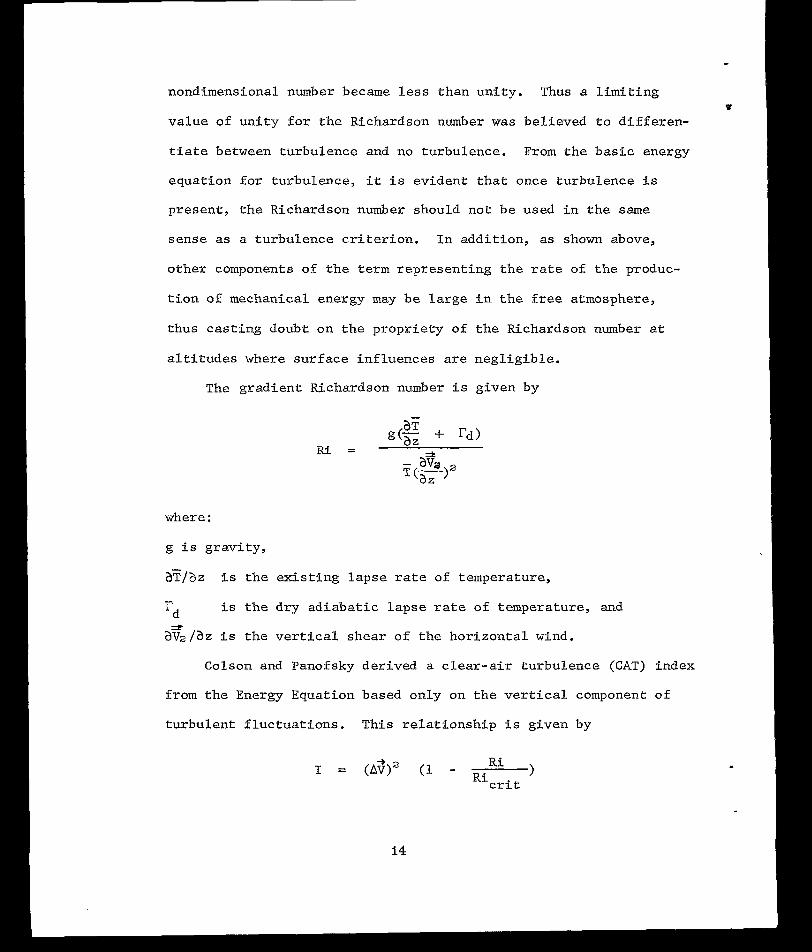
Colson and Panofsky derived a clear-air turbulence (CAT) index

from the Energy Equation based only on the vertical component of

turbulent fluctuations. This relationship is given by

1 = (A$)” (1 - 1 Ri Ricrit:

14

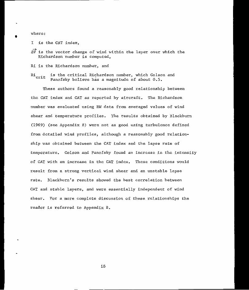
where :

I i s t h e CAT index,

AV i s the vector change of wind within the layer over which the +

Richardson number i s computed,

R i i s the Richardson number, and

Ricrit Panofsky believe has a magnitude of about 0.5. i s t h e c r i t i c a l R i c h a r d s o n number, which Colson and

mese authors found a reasonably good r e l a t ionsh ip between

t h e CAT index and CAT as reported by a i r c r a f t . The Richardson

number w a s evaluated using RW d a t a from averaged values of wind

shear and temperature prof i les . The resu l t s ob ta ined by Blackburn

(1969) (see Appendix B) w e r e not as good using turbulence defined

from de ta i l ed wind prof i les , a l though a reasonably good r e l a t ion -

sh ip w a s obtained between the CAT index and t h e lapse rate of

temperature. Colson and Panofsky found an i n c r e a s e i n t h e i n t e n s i t y

of CAT wi th an i nc rease i n t he CAT index. These condifsions would

r e s u l t f r o m a s t r o n g v e r t i c a l wind shear and an unstable lapse

rate. Blackburn 's resul ts showed the bes t co r re l a t ion between

CAT and s t ab le l aye r s , and were essent ia l ly independent of wind

shear. For a more complete discussion of these re l a t ionsh ips t he

reader i s r e fe r r ed to Appendix B.

15

V I . FIVALUATION OF STRESS/SHFAR TENSOR I N THE ENERGY EQUATION

The term involving the r a t e of mechanical production of

turbulence i n t h e e q u a t i o n on page 1 2 may b e w r i t t e n

which makes i t clear t h a t

r i j = -pu'u!. i J

The components o f t he stress tensor may b e i n t e r p r e t e d i n terms of

momentum t r anspor t which i s assumed to be p ropor t iona l to the mean

wind shear i n t h e a p p r o p r i a t e d i r e c t i o n . The j u s t i f i c a t i o n of t h i s

assumption i s t h a t t h e f l u x o f any quant i ty i s observed to be pro-

p o r t i o n a l t o t h e mean gradient of the quant i ty and i n a d i r e c t i o n

opposi te the mean gradient. Since i t i s observed that mean ver t ical

wind shears are much la rger than hor izonta l wind shears, even i n

the free atmosphere, i t appears permissible to express the shear

tensor as the sum of only th ree components which involve the verti-

c a l component of wind shear.

The covariances between fluctuations of t he u, v, and w wind

components, ufu!, can be evaluated from the detailed wind p r o f i l e

d a t a . I f i t i s assumed tha t t he dev ia t ions from the mean p r o f i l e ,

ui and u:, are composed of t rue wind f luc tua t ions and e r r o r , w e may

- 1 J

1

write

1 I ui = U i T + e i

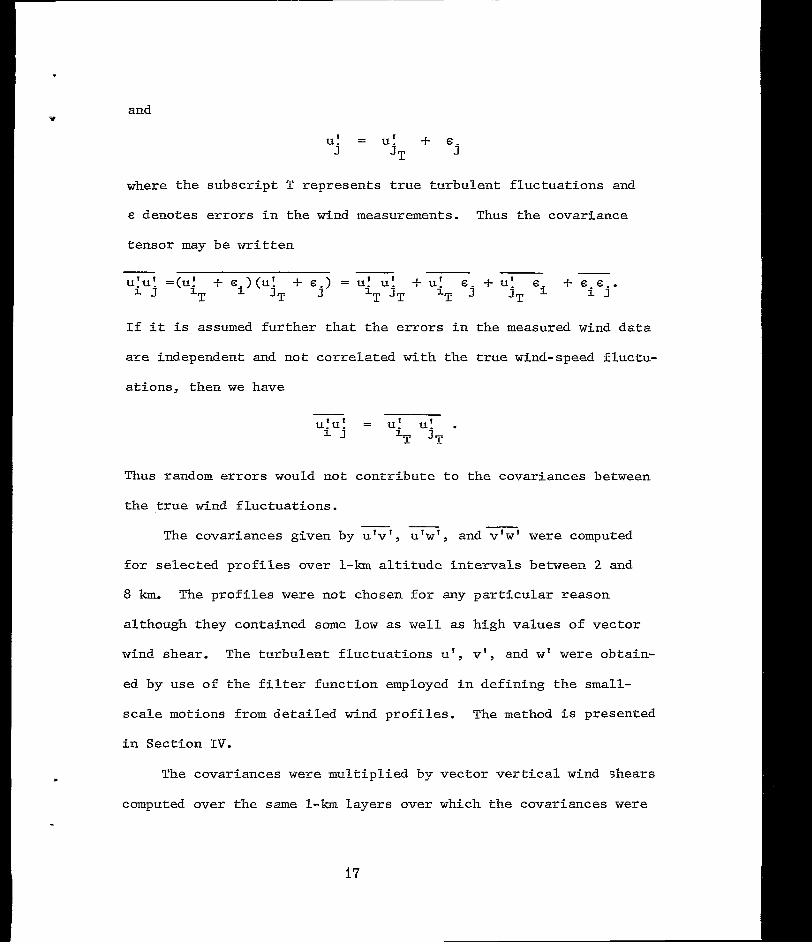
and

where the subsc r ip t T r ep resen t s t rue t u rbu len t f l uc tua t ions and

e deno tes e r ro r s i n t he wind measurements. Thus the covar iance

tensor may be wr i t ten

If it i s assumed f u r t h e r t h a t t h e e r r o r s i n t h e measured wind d a t a

are independent and not correlated w i t h the t r u e wind-speed fluctu-

a t ions, then we have

- ufu! = u! u' .

1 . J I T j T

the covariances between

-

Thus random e r r o r s would not cont r ibu te to

t h e t r u e wind f luc tua t ions .

The covariances given by u 'v ' , u'w', and v 'w ' w e r e computed

f o r se lec ted p rof i les over 1-km al t i tude in te rva ls be tween 2 and

8 km. The p r o f i l e s w e r e not chosen for any pa r t i cu la r r ea son

although they contained some low as w e l l as high values of vec tor

wind shear. The tu rbu len t f l uc tua t ions u', v ' , and w' w e r e obtain-

ed by u s e o f t h e f i l t e r f u n c t i o n employed i n d e f i n i n g t h e s m a l l -

scale motions from detailed wind p ro f i l e s . The method is presented

i n S e c t i o n I V .

"

The covariances w e r e mul t ip l ied by v e c t o r v e r t i c a l wind shears

computed over the same 1-km layers over which the covariances were

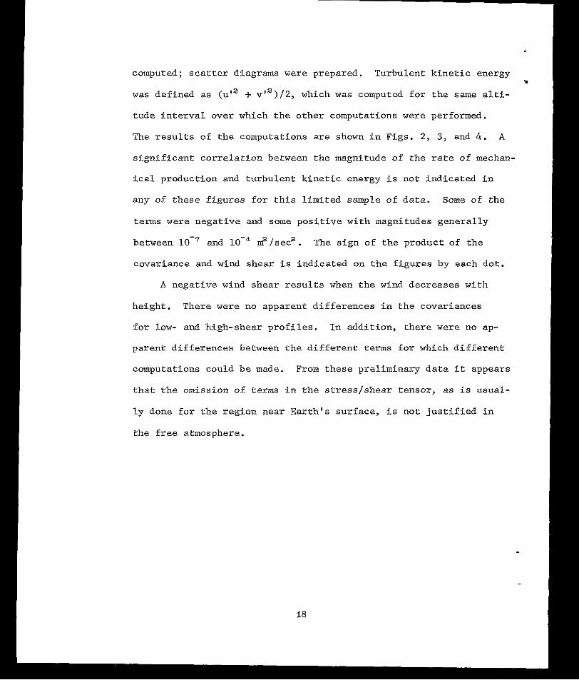
computed; scat ter d iagrams were prepared. Turbulent kinetic energy

w a s def ined as (u" f v t 2 ) / 2 , which was computed f o r t h e same al t i -

tude interval over which the other computations w e r e performed.

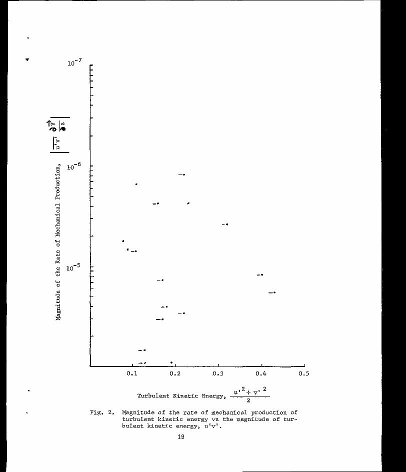
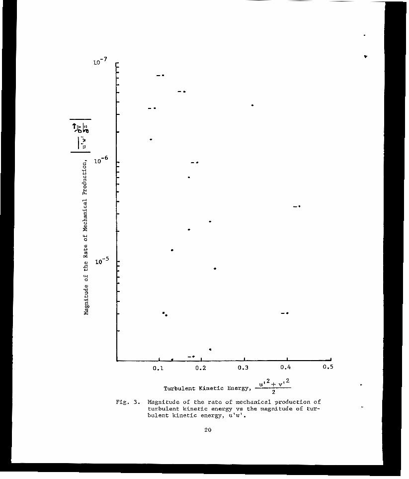
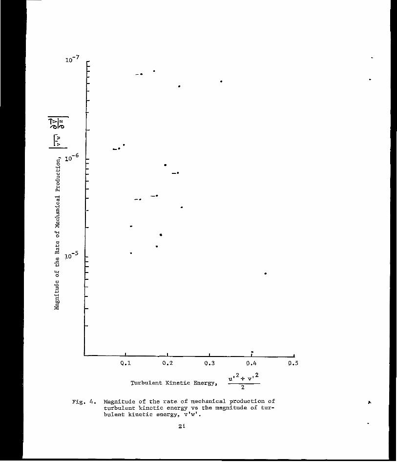
The results of the computations are shown i n F i g s . 2, 3, and 4 . A

s ign i f i can t co r re l a t ion between the magnitude of the rate of mechan-

ical production and turbulent kinet ic energy i s not ind ica ted in

any of these f igures €or th i s l imi ted sample of data . Some of the

terms w e r e negat ive and some posit ive with magnitudes generally

between and n-?/sec2. The sign of the product of the

covariance and wind shear i s indicated on the f i gu res by each dot.

A negative wind shea r r e su l t s when the wind decreases with

height. There were no apparent dif ferences i n the covariances

for low- and h igh-shear p rof i les . In addi t ion , there were no ap-

parent dif ferences between t h e d i f f e r e n t t e r m s €or which different

computations could be made. From these prel iminary data it appears

that the omission of terms in the s t ress jshear tensor , as is usual-

l y done for the region near Earth 's surface, i s n o t j u s t i f i e d i n

the free atmosphere.

-.

0

-. - * .

I 1 I I

0.1 0.2 0.3 0.4 0.5

U I 2 + v' 2 Turbulent Kinetic Energy, 2

Fig. 2. Magnitude of t he rate of mechanical production of t u rbu len t k ine t i c ene rgy vs the magnitude of t u r - bu len t k ine t ic energy , u 'v ' .

19

"

.

0

UJ + v' 2 Turbulent Kinetic Energy, 2

Fig. 3. Magnitude of the rate of mechanical production of turbulent kinetic energy vs the magnitude of turbulent kinetic energy, u'w'.

20

. ”

. s

.

Q.l 0.2 Q.3 0.4

2 a l l 2 + v’

Turbulent Kinet ic Energy, 2

Fig. 4 . Magnitude of t h e r a t e of mechanical production of tu rbulen t k ine t ic energy vs the magnitude of t u r - bu len t k ine t ic energy , v’w’.

21

0.5

I - V I I . RELATIONSHIPS BETWEEN SMALL-SCALE MOTIONS ASSOCIATED WITH DETAILED W I N D PROFILES AND SELECTED METEOROLOGICAL PARAMETERS

A . Lapse Rate of Temperature

Since the teams i n t h e Energy Equation involve wind shear and

l apse ra te of temperature, and since these parameters are included

i n t h e d e f i n i t i o n of the Richardson number, it i s log ica l t o cons i -

der these parameters as predictors o f turbulence. Various investi-

gators have obtained varying degrees of success.

The l apse rate of temperature computed from the RW da ta w a s

p lo t ted aga ins t the RMS turbulence values associated with the zonal

and mer2dional p rof i les for a l t i tude l ayers o f 250-, 500-, 1000-,

and 2000-m thickness with the top of each layer a t 6, 12, and 16 km.

These a l t i t u d e s were chosen to r ep resen t cond i t ions i n t he mid-

troposphere, i n t he t roposphe re nea r bu.t below the tropopause, and

i n t h e lower stratosphere. A scat ter diagram of aT/az versus RMS

zonal turbulence i s shown i n Fig. 5 f o r a n a l t i t u d e i n t e r v a l of

1000 m a t 12 km a l t i t u d e . Diagrams involving FQlS meridional turbu-

lence w e r e similar. There i s no apparent correlation between the

lapse r a t e of temperature and turbulence a t a l t i t u d e s of 6 and 1 6 km,

but there i s some suggestion of a s l i g h t c o r r e l a t i o n a t 12 km.

However, t h i s r e l a t i o n s h i p i s so poor t h a t i t may b e s t a t e d t h a t a

c o r r e l a t i o n between the l apse r a t e of temperature and turbulence

does not exist .

Q

22

h3 w

1.50

1.20

n 0 d)

2 0.90 W E

d) 0 d rl a,

1 P !-I

El rl a

=I 0.60

$ N

8 0.30

0.00

.

. . .

. #

. o

*

.

Fig. 5. The l apse r a t e of temperature computed over a layer of 1000 m vs RMS zonal turbulence for the same layer. The top of the layer was a t an a l t i t u d e of 1 2 km.

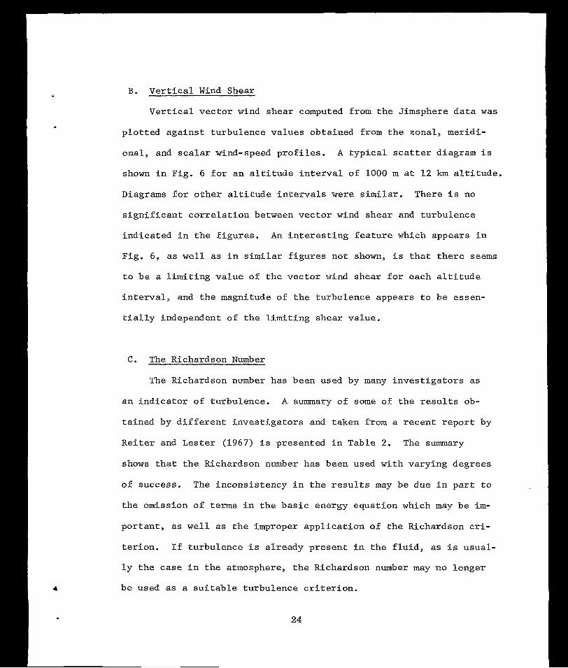
B. Ve r t i ca l Wind Shear

Vertical vector wind shear computed from the Jimsphere data w a s

p lot ted against turbulence values obtained from the zonal, meridi-

onal, and scalar wind-speed p r o f i l e s . A t y p i c a l scatter diagram i s

shown in F ig . 6 f o r a n a l t i t u d e i n t e r v a l o f 1000 m a t 1 2 km a l t i t u d e .

Diagrams f o r o t h e r a l t i t u d e i n t e r v a l s were similar. There i s no

s i g n i f i c a n t c o r r e l a t i o n between vector wind shear and turbulence

i n d i c a t e d i n the f igures . An i n t e r e s t i n g f e a t u r e which appears i n

Fig. 6, as w e l l as i n similar f igures no t shown, i s t h a t t h e r e seems

t o b e a l imi t ing va lue of the vec tor wind shear for each a l t i tude

i n t e r v a l , and the magnitude of the turbulence appears to be essen-

t i a l l y independent of the limiting shear value.

C. The Richardson Number

The Richardson number has been used by many inves t iga to r s as

an indicator of turbulence. A summary of some of t h e r e s u l t s ob-

tained by d i f f e r e n t i n v e s t i g a t o r s and taken from a recent report by

R e i t e r and Lester (1967) i s presented in Table 2. The summary

shows that the Richardson number has been used with varying degrees

of success. The i n c o n s i s t e n c y i n t h e r e s u l t s may be due i n p a r t t o

the omission of terms in t he bas i c ene rgy equa t ion which may be i m -

por tan t , as w e l l as t h e improper appl icat ion of the Richardson cri-

te r ion . I f tu rbulence i s a l r eady p re sen t i n t he f l u id , as i s usual-

l y t h e case i n t h e atmosphere, the Richardson number may no longer

be used as a su i tab le tu rbulence c r i te r ion .

24

n 0 al v1 \

v El

al 0 d aJ

rl a d 0 N

1.50

1.20

0.90

0.60

0.30

. *. *: . .. . .

. . . * * 7 . . . .

. . e . * . . B

. * .

*.

. . . .* . . * *..

.

Log [lo4 (aV/az> ] - 1000 m Jimsphere

lence for the same layer , The top of the layer was a t an a l t i t u d e of 1 2 km. Fig, 6 . The vec tor ver t ica l wind shear computed over a layer of 1000 m vs RMS zonal turbu-

. I

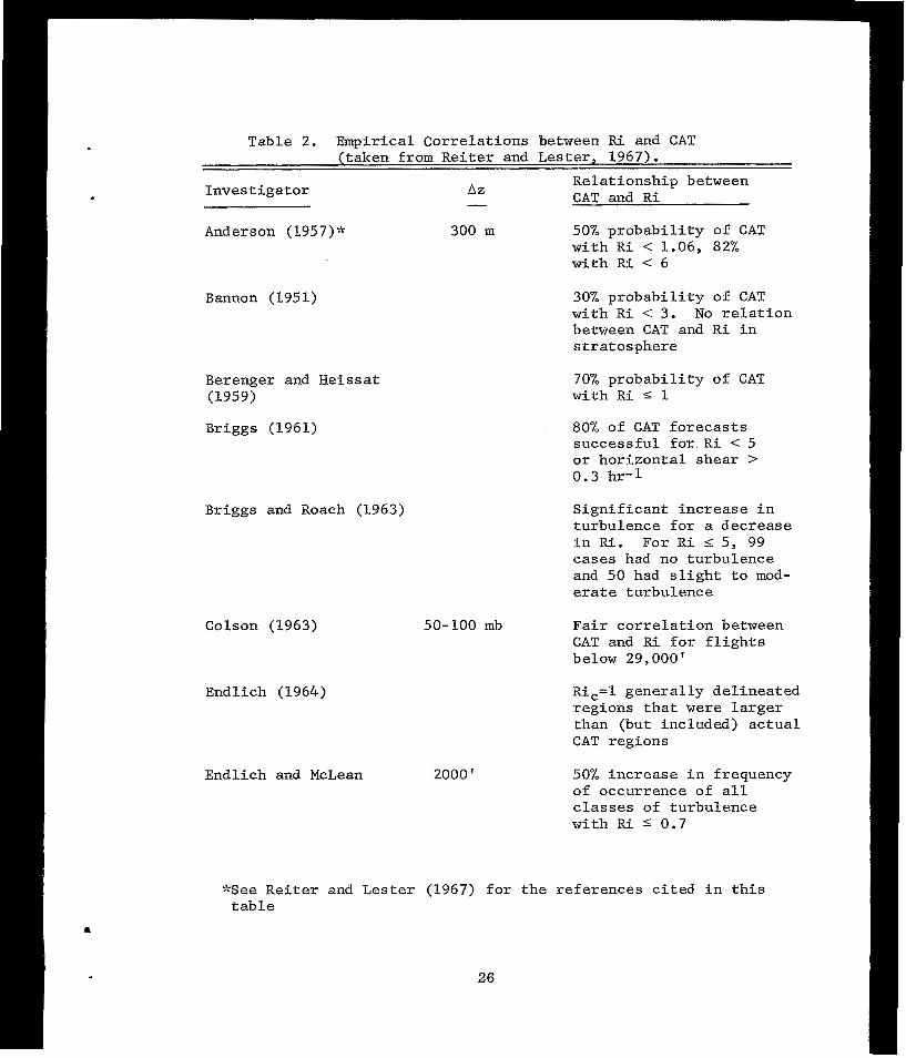
Table 2. Empirical Correlations between R i and CAT (taken from Reiter and Lester, 1967).

Relationship between Inves t iga to r A Z - CAT and R i

Anderson (1957)* 300 m 50% probabi l i ty o f CAT with R i < 1.06, 82% w i t h Ri 4 6

Bannon (1951)

Berenger and Heissat (1959)

Briggs (1961)

Briggs and Roach (1963)

Colson (1963)

Endlich (1964)

30% probabi l i ty o f CAT with R i < 3. No r e l a t i o n between CAT and R i i n s t ra tosphere

70% probabi l i ty o f CAT with Ri 5 1

80% of CAT fo recas t s successful for R i 4 5 or horizontal shear > 0.3 hr-1

S ign i f i can t i nc rease i n turbulence for a decrease i n R i . For R i I 5, 99 cases had no turbulence and 50 had s l i g h t t o moderate turbulence

50-100 mb F a i r c o r r e l a t i o n between CAT and Ri f o r f l i g h t s below 29,000'

R i c = l general ly del ineated reg ions tha t were l a rge r than (but included) actual CAT regions

Endlich and McLean 2000 ' 50% increase in f requency of occurrence of a l l classes of turbulence with R i 5 0.7

26

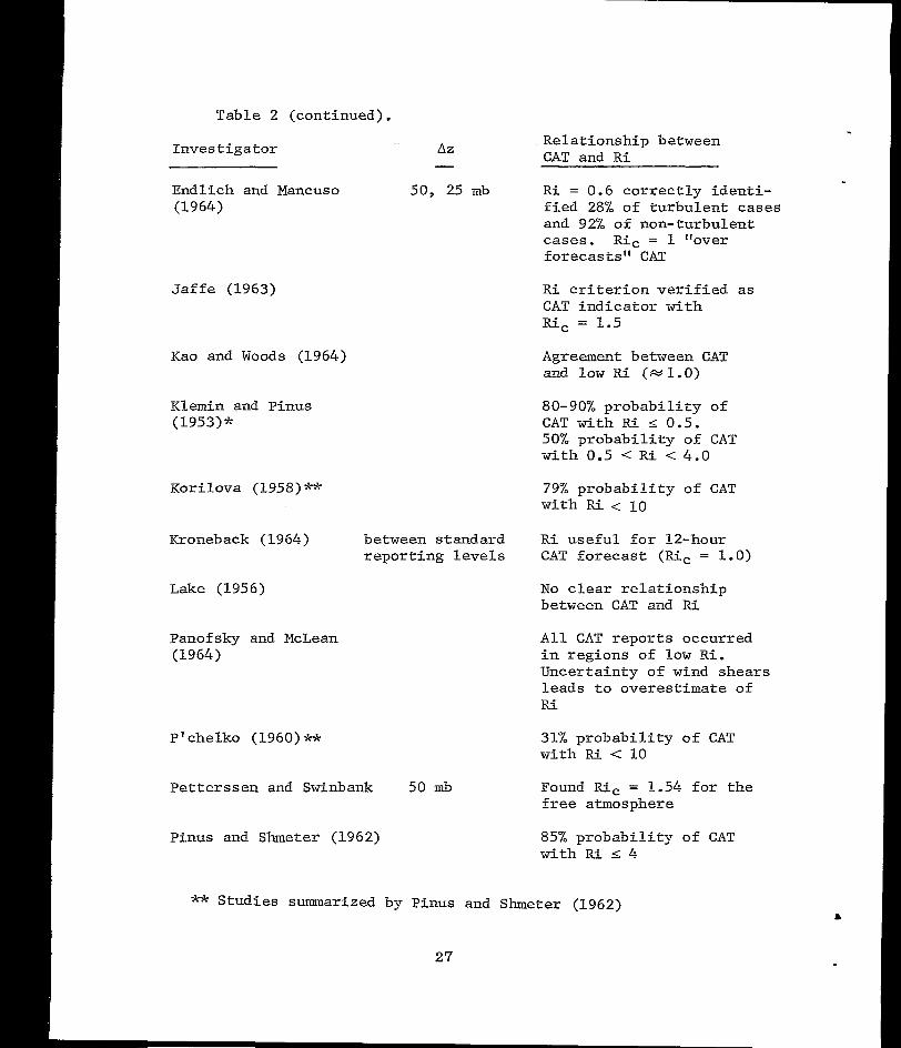
Table 2 (continued).

Inves t iga tor

Endlich and Mancuso (1964)

J a f f e (1963)

Kao and Woods (1964)

Klemin and Pinus (1953);;

Korilova (1958)**

Kroneback (1964)

Lake (1956)

Panofsky and McLean (1964)

P' chelko (1960) **

Relationship between CAT and R i

50, 25 mb R i = 0.6 co r rec t ly i den t i -

AZ -

f i e d 28% of turbulent cases and 92% of non-turbulent cases. R i c = 1 "over forecas ts" CAT

Ri c r i t e r i o n v e r i f i e d as CAT ind ica tor wi th R i c = 1.5

Agreement between CAT and l o w R i (-1.0)

80-90% probabi l i ty o f CAT with R i I 0.5. 50% probabi l i ty of CAT with 0.5 < Pci < 4.0

79% probabi l i ty o f CAT with R i < 10

between standard R i useful for 12-hour repor t ing levels CAT fo recas t (Ri, = 1.0)

N o c l ea r r e l a t ionsh ip between CAT and R i

A l l CAT reports occurred i n r e g i o n s of low R i . Uncertainty of wind shears leads to overestimate of R i

31% probabi l i ty o f CAT with Ri < 10

Pe t te rssen and Swinbank 50 mb Found Ric = 1.54 for t h e f r e e atmosphere

Pinus and Shmeter (1962) 85% probabi l i ty o f CAT with Ri 5 4

** Studies summarized by Pinus and Shmeter (1962) r

27

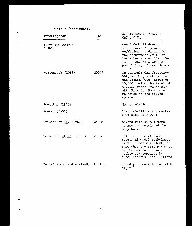
Table 2 (continued).

Investigator

Pinus and Shmeter (1965)

Rustenbeck (1963)

Scoggins ( 1 9 6 3 )

Scorer (1957)

2000 '

Stinson et al. (1964) 250 m "

Weinstein et al. (1966) 250 m

Zavarina and Yudin (1960) 1000 m

Relationship between CAT and Ri

Concluded: Ri does not give a necessary and sufficient .condition for the occurrence of turbulence but the smaller the value, the greater the probability of turbulence

In general; CAT frequency 64%, Ri s 5, although in the region 4000' above to 10,000' below the level of maximum winds 79% of CAT with Ri s 5. Poor correlation in the stratosphere

No correlation

CAT probability approaches 100% with Ri -S 0.01

Layers with Ri < 1 were common and persisted for many hours

Utilized Ri criterion (e.g. , Ri < 0.5 turbulent, Ri > 1.0 non-turbulent) to show that the strong shears can be maintained in a stable stratosphere by quasi-inertial oscillations

Found good correlation with Ric = 1

28

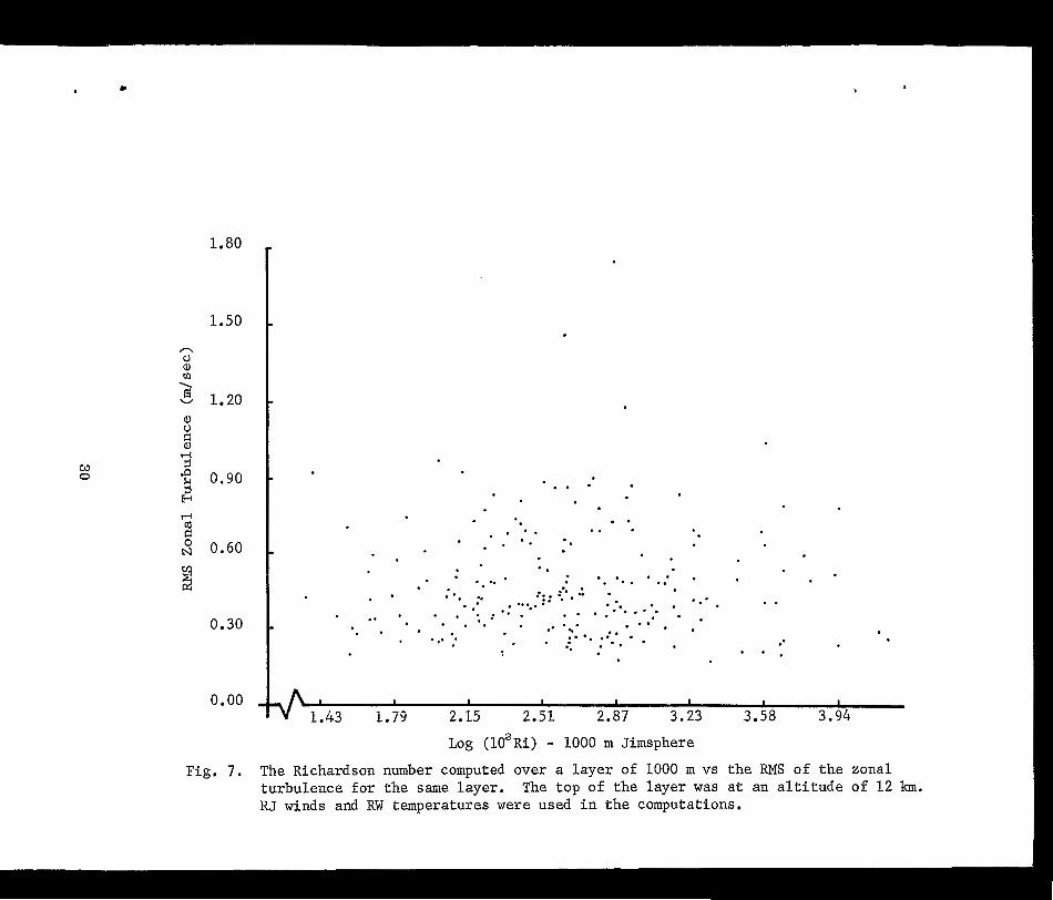
An inves t iga t ion w a s made of the re la t ionships between the

small-scale motions defined in Section IV and the Richardson number

( see a l so Appendix B). Computations were performed of the Richard-

son number and t h e RMS value of turbulence computed over layers of

var ious thicknesses with tops a t 6, 12, and 16 km. The Richardson

number plot ted against turbulence i s shown i n Fig. 7 f o r a se lec ted

case with the top of t he l aye r a t 12 km a l t i t u d e . The Richardson

number was computed over an a l t i tude in te rva l of 1000 m fo r t he ca se

shown. S i m i l a r r e s u l t s w e r e ob ta ined for o ther a l t i tude in te rva ls

and turbulence components. Even though the Richardson number has

been used widely as a c r i te r ion for tu rbulence , a cor re la t ion does

not ex i s t i n t he da t a cons ide red he re . A s po in ted ou t in Sec t ion V,

the Richardson number r e p r e s e n t s t h e r a t i o of only two t e r m s i n t h e

energy equation under the assumption that a l l o ther terms may be

neglected i n comparison. Results of the present investigation, as

w e l l as those summarized i n Table 2, suggest that th is assumption

may not be val id .

Relationships between CAT and the Richardson number o f t en are

in fe r r ed from t abu la r da t a r a the r t han scatter diagrams as presented

above. The relative frequency of balloon-measured turbulence ver-

sus the Richardson number, both computed over a l aye r 1000 m deep

and w i t h t o p s a t 6, 12, and 1 6 km, are shown i n Tables 3, 4, and 5.

29

0 0

1.80

1.50

1.20

0.90

0.60

0.30

0.00

Fig. 7.

. .

. .. .. . . . . .

. .

. .

I I I I I I I I

1.43 1.79 2.15 2.51 2.87 3.23 3.58 3.94

Log ( 102Ri) - 1000 m Jimsphere

The Richardson number computed over a layer of 1000 m vs the RMS of the zonal turbulence for the same layer, The top of the layer was a t an a l t i t ude of 12 km. RJ winds and RW temperatures were used i n t h e computations.

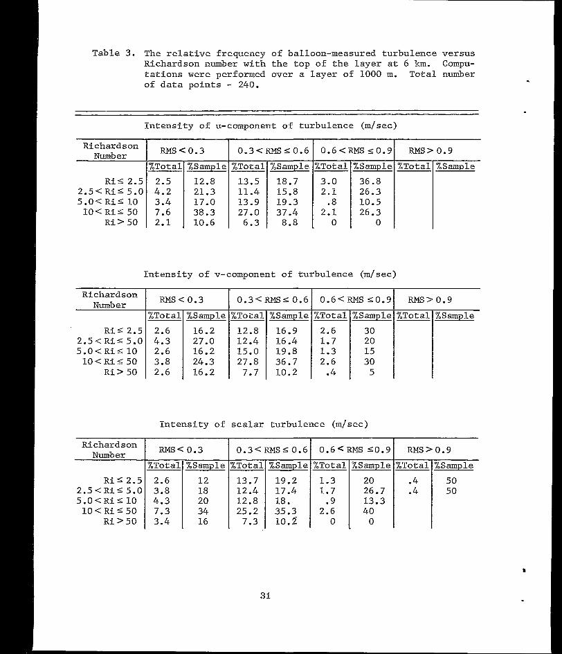
Table 3. The relative frequency of balloon-measured turbulence versus Richardson number w i t h t h e t o p o f t h e l a y e r a t 6 km. Compu- t a t i o n s w e r e performed over a layer of 1000 m, Total number of da ta po in ts - 240.

I n t e n s i t y of u-component of turbulence (m/sec)

Richardson Number

R i s 2.5 2 . 5 < R i r 5.0 5.0< R i r 10 IO< R i s 50

R i > 50

RMSc0.3

17.0 38.3

2.1 10.6

0.3<RMSs0.6 0.6<RMs 50 .9 RMS> 0.9

%Total %Sample %Total %Sample %Total %Sample

13.5 18.7 3.0 36.8 11.4 15.8 2.1 26.3 13.9 19.3 .8 10.5 27.0 37.4 2.1 26.3 6.3 8.8 , 0 0

In t ens i ty o f v-component of turbulence (m/sec)

Richardson Number RMS< 0.3 0.3<RMsS 0.6 0.6< RMS r 0 . 9 RNS> 0.9

%Total %Sample %Total %Sample %Total %Sample %Total %Sample

R i I 2.5 2.6 16.2 12.8 16.9 2.6 30 2 .5CRi55.0 4.3 27.0 12.4 16.4 1.7 20 5 . 0 < R i r 10 2.6 16.2 15.0 19.8 1.3 15

1 0 < R i 5 5 0 3 . 8 24.3 27.8 36.7 2.6 30 R i>50 2.6 16.2 7.7 10.2 .4 5

In t ens i ty o f scalar turbulence (m/sec)

Richardson Number RMs< 0.3 O.3<RMS5O0,6 0.6CRMS S0.9 RMs>O.9

%Total %Sample %Total %Sample %Total %Sample %Total %Sample

R i r 2 . 5 2.6 12 13.7 19.2 1.3 20 .4 50 2 . 5 < R i I 5.0 3.8 18 12.4 17.4 1.7 26.7 .4 50 5 . 0 c R i I 1 0 4.3 20 12.8 18. .9 13.3

l O < R i 5 5 0 7.3 34 25.2 35.3 2.6 40 R i>50 3.4 16 7.3 10.2 0 0

31

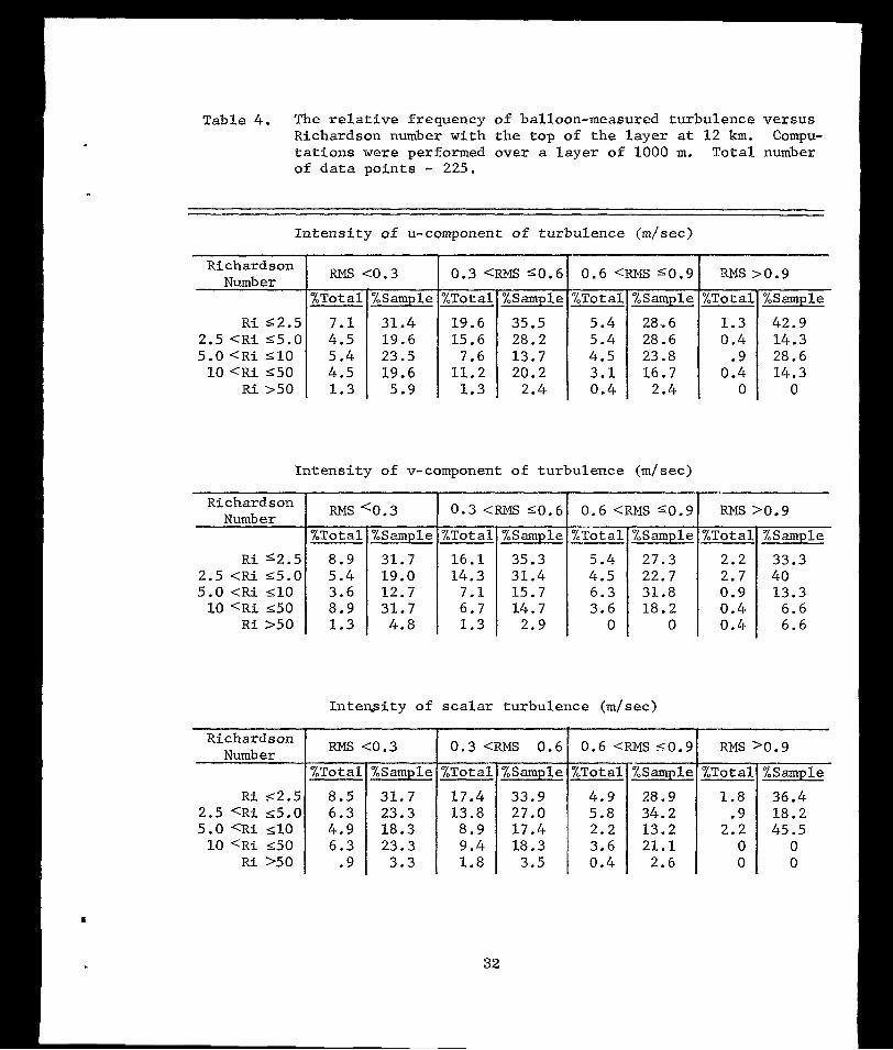
Table 4. The relat ive f requency of balloon-measured turbulence versus Richardson number wi th the top of the l ayer a t 1 2 km. Compu- t a t i o n s were performed over a layer of 1000 m. Total number of da t a po in t s - 225.

I n t e n s i t y of u-component of turbulence (m/sec)

Richard son Number

%Total

R i s 2 . 5 7 . 1 2.5 < R i 55.0 4 .5 5 .0 < R i 510 5 . 4

10 < R i s50 4 .5 Ri >50 1 .3

< :o .3 0.3 <RMS S0.6 0 .6 <

%Sample %Total %Sample %Total

31.4 19.6 35.5 5.4 19.6 15.6 28.2 5.4 23.5 7.6 13.7 4.5 19.6 11 .2 20.2 3.1

5.9 1.3 2.4 0 .4

23.8 16.7

2.4

I n t e n s i t y of v-component of turbulence (m/sec)

R i s2 .5 8 .9 2.5 < R i s 5 . 0 5 . 4 5.0 <Ri 210 3.6 10 < R i 550 8 .9

R i >50 1.3

%Sample %Total %Sample % T o z

31.7 16 .1 35.3 5 .4 19.0 14.3 31.4 4.5 12.7 7 .1 15.7 6.3 31.7 6.7 14.7 3.6

4 .8 1 .3 2 .9 0

Richardson Number RMS <0.3 0.3 <RMS 50 .6 0.6 <RMS sO.9 RMS >0,9

%Total %Sample

27.3 22.7 31.8 18.2

0

.0.9

%Sample

42.9 14.3 28.6 14.3

0

%Sample

33.3 40 13.3

6.6 6.6

In tens i ty o f sca la r tu rbulence (m/sec)

Ri ~ 2 . 5 8.5 2.5 <Ri 55.0 6 .3 5.0 <Ri 5 1 0 4 . 9

10 <Ri ~ 5 0 6.3 R i >50 .9

ZSample

31.7 23.3 18.3 23.3

3.3

pij %Total

17.4 13.8

8.9 9.4 1.8

33.9 4.9 27.0 5.8 17 .4 2 .2 18.3 3.6

3 .5 0 .4

28.9 1.8 34.2 .9 13.2 2.2 21.1 0

2.6 0

'/,Sample

36.4 18.2 45.5

0 0

32

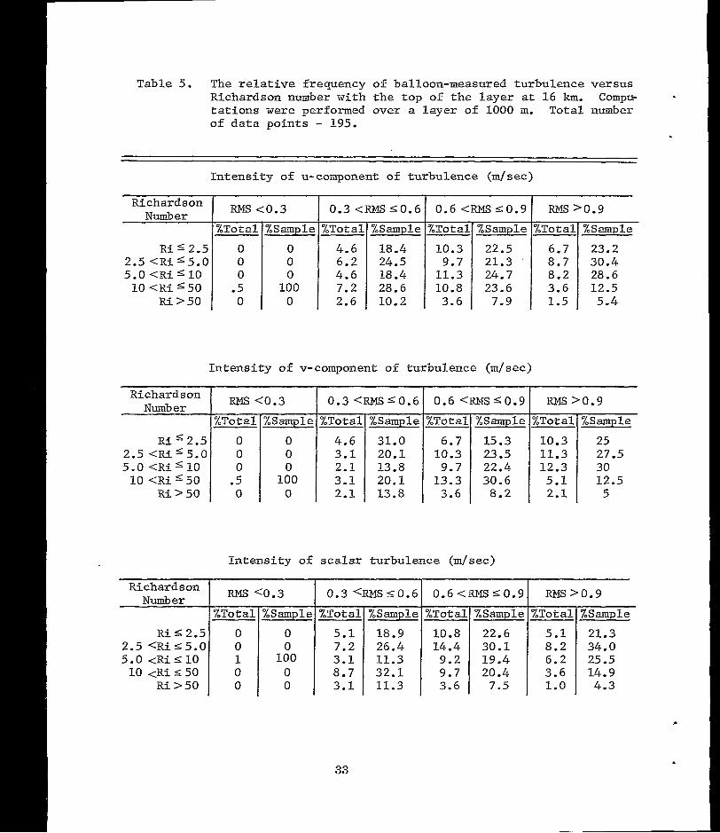
Table 5. The relative frequency of balloon-measured turbulence versus Richardson number wi th the top of t h e l a y e r a t 16 km. Compu- t a t i o n s w e r e performed over a layer of 1000 m. Tota l number of d a t a p o i n t s - 195.

I n t e n s i t y of u-component of turbulence (m/sec )

R i 5 2 . 5 0 2.5 < R i I 5 . 0 0 5.0 <Ris 10 0

1 0 < R i 5 5 0 .5 Ri > 50 0

Richardson Number RMS <o.3

%Total , %Sample

0 0 0

100 0

T 0.3 <RMS 50.6

28.6 10.2

T 0.6 "S 5 0 . 9

%Total

10.3 9.7

11.3 10.8 3.6

%Sample

22.5 21.3 24.7 23.6

7.9

I n t e n s i t y of v-component of turbulence (m/sec)

T RNS >0.9

5.4

Richardson Number RMS <0.3 0.3 <RMSS0.6 0.6 <RMS 50 .9 RMS >0.9

%Total'%Sample %Total %Sample %Total %Total %Sample %Sample R i s2 .5 0 0 4.6 31.0 6.7

12.3 30 22.4 5.0 < R i LO 0 0 2.1 13.8 9.7 11.3 27.5 23.5 2.5 <Ri 5.0 0 0 3.1 20.1 10.3 10.3 25 15.3

10 < R i 50 .5 100 3.1 20.1 13.3 30.6 5.1 12.5 R i > 50 0 0 2.1 13.8 3.6 8.2 2.1 5

I n t e n s i t y of scalar turbulence (m/sec)

Richardson Number RNS C0.3 0.3 <RMS 50 .6 0.6 <I% 5 0 . 9 RMS >0.9

%Total %Sample %Total %Sample %Total %Total %Sample %Sample R i 5 2.5 0 0 5.1 18.9 10.8

19.4 5.0 < R i I 10 1 100 3.1 11.3 9.2 8.2 34.0 30.1 2.5 K R i s 5 . 0 0 0 7.2 26.4 14.4 5.1 21.3 22.6

6.2 25.5 10 <Ri I 50 0 0 8.7 32.1 9.7 20.4 3.6 14.9

R i >50 0 0 3.1 11.3 3.6 7.5 1.0 4.3

c

33

Table 3 presents relationships between the frequency of occur-

rence of turbulence, magnitude of the turbulence, and the Richardson

number for turbulence associated with the zonal (u), meridional

(v), and scalar wind prof i les . Table 3 r e f e r s t o t h e l a y e r 5-6 km,

Table 4 t o t h e l a y e r 11-12 km, and Table 5 t o t h e l a y e r 15-16 km.

The 'I% Total" column g ives the percentage o f the to ta l number of

observations in each category, while the 11% Sample" column gives

the percentage of observat ions in each category of Richardson num-

be r fo r t he g iven i n t ens i ty of turbulence. Thus t h e sum of a l l

l r% Total" columns i n each cable should be loo%, as should the sum

of each Sample" column.

Based on data presented by Susko and Vaughan (9. s.) and Scog-

gins (1967), i t appears reasonable to assume t h a t RMS turbulent

f luc tua t ions wi th a magnitude less than 0.6 m / s e c are caused largely

by e r r o r s i n t h e measurement system. RMS values greater than 0 .6

m/sec would then i nd ica t e the presence of turbulence.

I n a study of clear a i r turbulence, Colson and Panofsky (OJ. &.I

present data which show t h a t CAT occurs between approximately 3 t o

18% of t he t i m e a t p re s su re a l t i t udes between 500 and 200 mb based

on a i r c r a f t d a t a . The percentage increases from 3 t o 18% with an

i n c r e a s e i n wind shear which would be equivalent to a d e c r e a s e i n

the Richardson number. This compares with the range of approxi-

mately 10-25% i n Tables 3 and.4 when the tu rbulence in tens i ty i s be-

tween 0.6 and 0.9 m/sec. At higher a l t i tudes (Table 5) the percen-

tages are considerably larger , suggest ing that errors may be l a rge r

34

o r t h e r e i s a greater frequency of the occurrence of turbulence.

Based on the appearance of the measured profiles, one i s l e d t o

suspec t tha t l a rger sys tem e r rors a re respons ib le €or the ind ica ted

l a r g e r t u r b u l e n c e i n t e n s i t i e s a t t h e h i g h e r a l t i t u d e s .

It cannot be s ta ted conclusively that turbulence can be detec-

t e d and i t s i n t e n s i t y measured by t h e R J system until simultaneous

and quant i ta t ive a i rc raf t o r o ther independent da ta a re ava i lab le .

However, t he above r e s u l t s , which agree so c losely with those

presented by Colson and Panofsky and based on a i r c ra f t da t a , sugges t

that turbulence can be detected by t h e system.

The lapse ra te of temperature and the ve r t i ca l shea r o f t he

hor izonta l wind are impor tan t parameters in the def in i t ion o f the

Richardson number. Temperature l a p s e r a t e i s not as c r i t i c a l a s

wind shear s ince i t en te r s t o t h e first power, whereas wind shear

e n t e r s t o t h e second power. In add i t ion , t he l apse r a t e o f temper-

a t u r e computed by f i n i t e d i f f e r e n c e s o v e r l a y e r s of d i f f e r e n t

thicknesses does not vary as much a s t h e v e r t i c a l wind shea? measured

over the same layers . Thus, the shape of the wind p r o f i l e and the

thickness of the layer over which the computations are performed

may p roduce l a rge va r i a t ions i n t he computed Richardson number.

For example, it i s p o s s i b l e f o r t h e wind shear to be l a rge over a

layer of 500 m and small over a layer of 2000 m wi th in the same

p r o f i l e and overlapping layers. The depth of the layer over which

the computations should be performed i s not known. Some aspects of

t h i s problem are presented below.

.

35

The influence of more accurate wind p r o f i l e d a t a i n computa-

t ions of the Richardson number i s i l l u s t r a t e d i n F i g . 8 where

Richardson numbers computed with RW and R J winds are compared. As

shown i n t h e f i g u r e , wind shear has an important influence on t h e

magnitude of the Richardson number. The dispers ion of the po in ts

i s due to the inf luence of small -scale motions present in the RJ

wind p r o f i l e s which are no t p re sen t i n t he RW wind prof i les . Fig. 9

i s similar t o Fig. 8 but with wind shears calculated over a layer

2000 m i n depth. The agreement i s much b e t t e r , as might be expec-

ted, since both systems measure wind shears over deep layers with

approximately the same accuracy. The influence of wind shears

measured over d i f f e r e n t a l t i t u d e i n t e r v a l s on the Richardson number

i s i l l u s t r a t e d i n F i g . 10, where Richardson numbers computed over

500 m are compared with those computed over a layer of 2000 m i n

depth. There i s very l i t t l e , i f any, c o r r e l a t i o n between t h e

Richardson number computed over the two l aye r s even though t h e

top of each layer w a s a t t he same a l t i t u d e .

Figure 11 demonstrates that wind shear measured over different

a l t i t u d e l a y e r s i s p r imar i ly r e spons ib l e fo r va r f a t ions i n t he

Richardson numbers computed over the var ious layers . The disper-

sion of points i n Figs. 10 and 11 i s la rge , ind ica t ing the poor

r e l a t ionsh ip between wind shears computed over d i f fe ren t l ayers .

36

4*30 I- I

. .

I I 1 1 1 I ,43 1.79 2.15 2.51 2.87 3.23 3.58

Log (l@Ri) - 500 Jimsphere

Fig. 8. The Richardson number computed over a layer of 500 m with RJ winds vs the Richardson number computed over the same layer with RW winds. The top of the layer was a t an a l t i t ude of 12 km.

,

L

0 0

0 0 00 w

bo 0 Ki

4.30

3.87

3.44

3.01

2.58

2.15

1.72

. . . .

. . . . a . . .

G

I I I

1.79 2.15 2.51 2.87 3.23 3.58 2.94 4.30

Log (l$Ri) - 2000 m Jimsphere

Fig. 9. The Richardson number computed from RJ winds and RW temperatures vs the Richardson number computed from RW winds and temperatures. The computations were performed over a layer of 1000 m with the top of the layer at 1 2 km.

D. Parameters Determined From Synoptic Charts

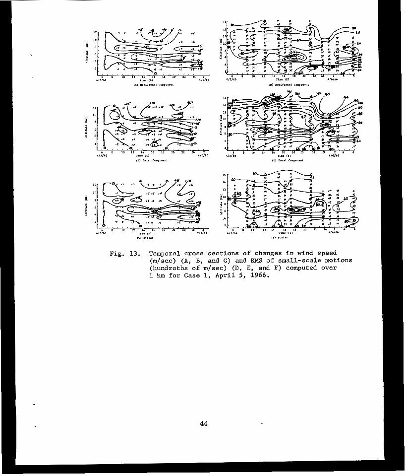
Temporal c ros s s ec t ions o f t he RMS value of turbulence deter-

mined ove r a l t i t ude i n t e rva l s of 1 km for the meridional , zonal ,

and scalar wind-speed p r o f i l e s , and changes i n the corresponding

wind speeds t o an a l t i t ude of 1 2 km were prepared. In addition,

synopt ic char ts w e r e prepared from RW d a t a f o r t h e 850-, 700-,

500-, 400-, 300-, and 200-mb levels wi th da t a measured at t i m e s

corresponding to the temporal cross sect ions. For ident i f icat ion

purposes these are cal led: C a s e 1 ( A p r i l 5, 1966); Case 2 ( A p r i l 8,

1966) ; C a s e 3 (July 5 , 1966), and; Case 4 (September 16, 1966).

The maps and cross sec t ions are shown i n F i g s . 12-19, which are

shown i n t h e s e c t i o n i n which each i s discussed.

The temporal cross sections of changes i n wind speed represent

the change tha t took p lace be tween the f i r s t p rof i le i n t h e series

and each p ro f i l e t he rea f t e r . The change that took place between

any two success ive p rof i les i s the d i f f e rence between the va lues

g iven fo r t he p ro f i l e s i n t he c ros s s ec t ion . C a r e must be exercised

in t he i n t e rp re t a t ion o f t hese f i gu res . Fo r example, t h e h o r i z o n t a l

g rad ien t o f the i so l ines p resented in the c ross sec t ions w i l l b e

g r e a t e s t when the change between successive profiles i s g rea t e s t ,

b u t i n t h e c a s e where the wind speed did not change with t i m e a t a

g i v e n a l t i t u d e , t h e i s o l i n e s will be horizontal . The temporal

c ross sec t ions represent ing the small-scale motions present an

ana lys i s o f the RMS value of the motions over 1-km a l t i t u d e i n t e r -

va l s fo r each p ro f i l e at t h e t i m e indicated. Thus l a rge ho r i zon ta l

41

gradien ts on these cross sect ions a lso represent a l a rge change i n

the p roper t ies of the small-scale motions with t i m e , and i n t h i s

respect may be i n t e rp re t ed i n a similar manner as the temporal

c ross sec t ions of changes i n t h e wind speed. This method of

presenta t ion w a s chosen because i t was e a s y t o v i s u a l i z e a l t i t u d e

reg ions wi th h igh pers i s tence in the wind speeds as w e l l as regions

where changes take place i n t h e observed intensity of small-scale

mot ions . In the in te rpre ta t ions o f the f igures i t should be kept

i n mind t h a t t h e changes of wind speed can be measured quite accu-

ra te ly wi th the RJ system but that RMS values of leas than ca. 0.6

m/sec in the small-scale motions cannot be detected with certainty.

Because o f the l a rge var ia t ions observed in the cases s tud ied , each

one w i l l be consldered separately.

Case 1 (Figs. 1 2 and 13). Strong cold advection is indicated

a t 122 below an a l t i t u d e of 400 mb, with weak cold advection a t

400, 300, and 200 mb. Twelve hours later, cold advection s t i l l

pers i s ted a t a l l levels from 300 mb and below, with warm advection

a t 200 mb. The wind backed wi th he ight a t bo th times as i t should

when cold advection i s occurring. When the winds back with height,

and i f t h e i n i t i a l wind is from t h e west, one might expect the zonal

component to decrease in magni tude with t i m e . This was not obser-

ved. Whether o r no t t he component wind speeds increased or decreased

apparently depended upon the increase o r decrease in the magni tude

of t he s ca l a r wind speed. This of course i s r e l a t e d t o t h e magni-

tude of the pressure gradient force which, in turn, is r e l a t e d t o

42

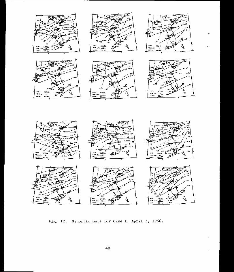
Fig. 12. Synoptic maps for C a s e 1, April 5, 1966.

43

12

LO

8

6

k

2

4 / 5 / 6 6 T l r (21 416166 (C) sc.1.r

Fig.' 13. Temporal cross sections of changes in wind speed (m/sec) (A, By and C) and RMS of small-scale motions (hundreths of m/sec) (D, E, and F) computed over 1 km f o r Case 1, A.pril 5, 1966.

44

the gradient of the mean vir tual temperature below t h e l e v e l i n

question. An examination of the indicated advective change i n

temperature compared w i t h the ac tua l change i n temperature for

Tampa revealed that the sign of the measured change was the same

as the s ign for the advect ive change but of a smaller magnitude.

Thus, i n t h i s c a s e t h e s l o p e of a given isobaric surface might

differ considerably from t h a t which would be calculated only on

the basis of advective change in temperature. The observed changes

i n t h e magnitude of the component wind speeds were as high as

13 m/sec over a period of 1 2 hours b u t general ly were between 2

and 6 m / s e c .

Case 2 (Figs. 14 and 15). In this case the advect ion of

temperature was not pronounced, however the observed changes be-

tween 00 and 122 w e r e g rea t e r t han i n Case l where the advective

change was much greater. There was cold advect ion in Case 2 below

400 mb and the winds w e r e observed t o back with height. But again

the behavior of the meridional and zonal components appeared to be

influenced by the magnitude of the vector wind and thus-did not

change i n a systematic manner. Between 00 and 122, t he l a rges t

changes w e r e observed below an a l t i t u d e of 5 Jan (about 500 mb) and

reached a magnitude for the meridional component of 11 m/sec.

Between 12 and OOZ t h e l a r g e s t changes occurred above an altitude

of 8 km where the zonal component decreased as much as 10 m/sec.

The changes observed i n Case 2 would not have been predicted on

45

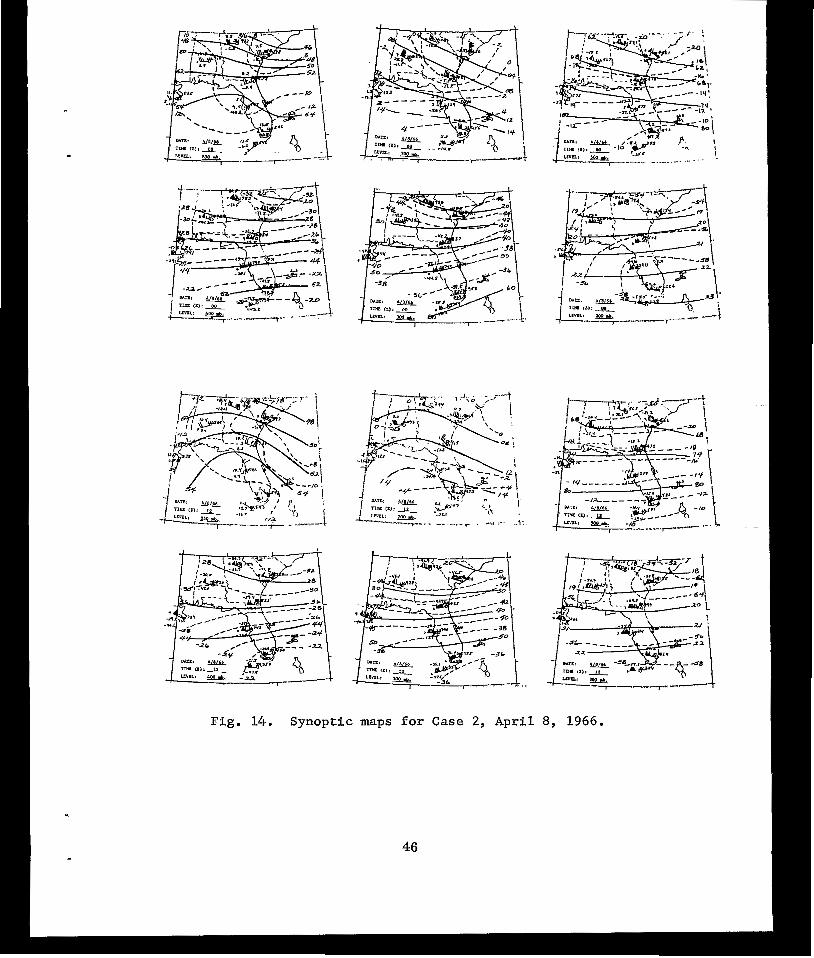
Fig. 14. Synoptic maps for Case 2, April 8, 1966.

46

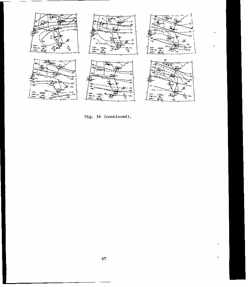
Fig. 14 (continued).

47

A11166 4 / 9 / 6 6

Fig. E. Temporal cross sections of changes in wind speed (m/sec) (A, B, and C) and RMS of small-scale motions (hundreths of m/sec) (D, E, and F) computed over 1 km for Case 2, April 8, 1966.

the basis of a change i n t h e mean virtual temperature of the air

column as indlcated by advection.

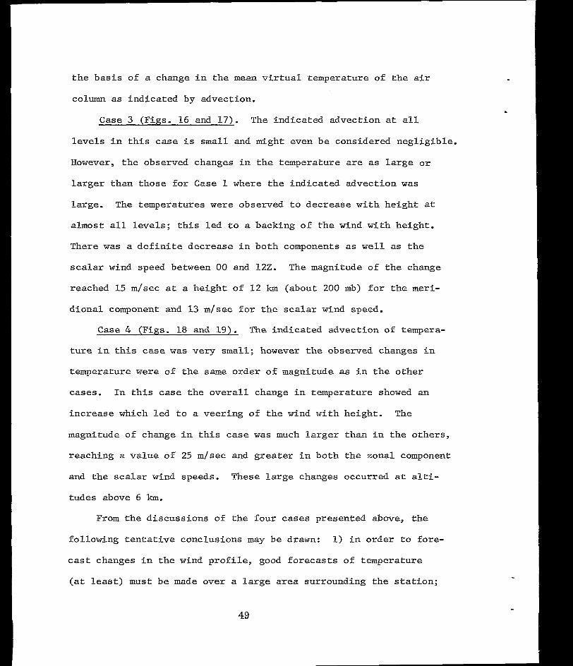
C a s e 3 (Figs. 16 and 17) . The indicated advect ion a t a l l

l e v e l s i n t h i s case i s s m a l l and might even be considered negligible.

However, the observed changes i n the temperature are as l a r g e o r

larger than those for C a s e 1 where the indicated advect ion w a s

large. The temperatures were observed to decrease with height a t

almost a l l Levels ; th is led t o a backing of the wind with height .

There was a d e f i n i t e d e c r e a s e i n b o t h components as w e l l as t h e

scalar wind speed between 00 and 12Z. The magnitude of the change

reached 15 m / s e c a t a height of 1 2 km (about 200 mb) f o r t h e m e r i -

d iona l component and 13 m / s e c f o r t h e scalar wind speed.

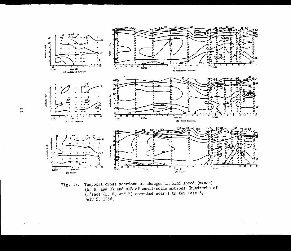
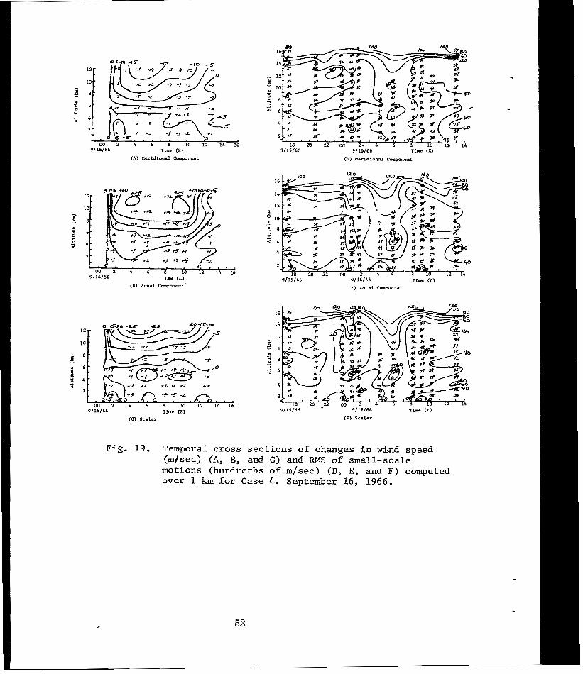
Case 4 (Figs. 18 and 19) . The indicated advect ion of tempera-

t u r e i n t h i s case w a s very s m a l l ; however the observed changes i n

temperature w e r e o f the same order o f magnitude as i n the o the r

cases. In t h i s case the overa l l change in t empera ture showed an

inc rease which led t o a veer ing of the wind with height . The

magnitude of change i n t h i s case w a s much l a rge r t han i n t he o the r s ,

reaching a value of 25 m/sec and g r e a t e r i n b o t h t h e z o n a l component

and the scalar wind speeds. These large changes occurred a t a l t i -

tudes above 6 'km. From the discussions of the four cases presented above, the

fol lowing tentat ive conclusions may be drawn: 1) i n o r d e r t o Eore-

cast changes i n t h e wind p r o f i l e , good fo recas t s of tempera ture

(at l e a s t ) must be made over a l a r g e area surrounding the s ta t ion;

49

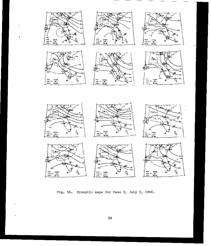
Fig. 16. Synoptic maps for Case 3, July 5, 1966.

50

::I

t On 6 111 20 22 00 713116 1/4/66

Fig. 18. Synoptic maps for Case 4 , September 16, 1966.

52

M) 2 4 6 8 10 12 14 16 9 / 1 6 / 6 6 Time (2) 9 16/66 Tire (2)

(C) Scalar

Li 16

Fig. 19. Temporal cross sections of changes in w i d speed (m/sec) (A, B, and C) and RMS of small-scale motions (hundreths of m/sec) (D, E, and F) computed over 1 Jan for Case 4 , September 16, 1966.

. 53

2) the cor rec t s ign of a change i n t h e wind d i r ec t ion i s determined

apparently by the sign of the observed change i n temperature; back-

ing of the winds i s associated with cold advection while veering

i s associated with warm advection, and; 3 ) t he magnitude of the

observed change in the temperature over per iods of 12 hours and

grea te r i s not given by advection. Advection of temperature over

shorter t ime periods and the inf luence of ver t ical motion on the

prediction of winds are t r e a t e d i n S e c t i o n V I I I .

An attempt w a s made to de te rmine the re la t ionships , i f any,

between the RMS values of the small-scale motions and 1) horizon-

t a l wind shear, 2) curvature of the f low (cyclonic or ant i -cyclonic) ,

3) advection of temperature, 4 ) loca t ion and in t ens i ty of the

j e t stream, 5) v o r t i c i t y , and 6 ) advect ion of vort ic i ty . The

f i r s t f o u r of these parameters w a s calculated from the 700-, 500-,

and 300-mb c h a r t s i n all cases and the last two parameters from

t h e 500-mb charts. Large values of hor izonta l wind shear in cases

of both cyclonic and ant i -cyclonic curvature were observed, as w e l l

as large negat ive and pos i t ive va lues of both temperature and vo r t i -

c i ty advect ion. The magnitude of the vort ic i ty a t 500 mb varied

between 4 and 8 x 10- sec with some values cyclonic and some

anti-cyclonic. While some o f the observed changes i n t he Rp4S

values of the small-scale motions were much larger than those ex-

pected from error, scatter diagrams did not reveal any systematic

relationships between the parameters investigated and the magni-

5 -1

54

tude of the turbulent deviat ions. It appears that the r e l a t ion -

sh ips between synoptic-scale parameters and small-scale motions

are so complex that i t i s n o t p o s s i b l e t o relate t h e two by con-

sidering simple parameters obtained from individual constant-

pressure char ts . A much more complicated approach i s required

which cons iders the in te rac t ion between var ious layers . Addi t ional

research i s required to e s t a b l i s h these re la t ionships .

55

V I I I . A SIMPLE METHOD FOR FORECASTING THE W I N D PROFILE

.A. Introduct ion and Background of Problem

Forecasts of detai led wind p r o f i l e s are of prime concern to

both meteorologists and engineers. Wind shear and turbulence are

important i n t h e d e s i g n and operation of space vehicles. Ryan,

Scoggins, and King ~~ (1967) invest igated the inf luence of small-scale

(vertical wavelengths less than 1000 m) wind shears on the design

of space vehicles. They demonstrated that small-scale wind shears

inf luence s ignif icant ly the control system as w e l l as the bending

moments experienced by the vehicle .

S p a t i a l and tempora l var ia t ions in small-scale winds are not

known accurately. Thus, when a space vehicle i s launched through

t h e ( p a r t i a l l y ) unknown wind f i e l d , a low r i s k must be accepted

t h a t t h e v e h i c l e w i l l be l o s t (Vaughan, 1968). This r i s k might be

r educed s ing i f i can t ly i f t he wind prof i le could be forecas t ac-

cura te ly .

In addi t ion to the impor tance o f wind p ro f i l e s i n t he des ign

and operation of space vehicles, consideration of them i s s i g n i f i -

c a n t i n many meteorological problems (Panofsky, 1956; Hess, 1959).

Vertical shears of the hor izonta l wind are r e l a t e d t o clear-alr

turbulence and are important i n exchange processes which relate

d i r ec t ly t o a tmosphe r i c d i f fus ion and t o t h e flux of quant i t ies

through the atmosphere (Lumley and Panofsky, 1964; Reiter, 1963).

In add i t ion , wind shear i s re la ted to the thermal s t ruc ture o f the

atmosphere which, i n t u r n , i s r e l a t e d t o many dynamical and thermo-

dynamical processes (PEtterssen, 1956). Thus wind shear i s an

impor tan t cons idera t ion in many p r a c t i c a l as w e l l as t h e o r e t i c a l

problems.

Most wind p r o f i l e s now a v a i l a b l e a r e "smooth" because the

small-scale f luc tua t ions have been f i l t e red ou t due to the smooth-

i ng i nhe ren t i n t he ca l cu la t ions o f t he RW wind data . ' A few

s t a t i o n s now have an RJ system which provides "detailed" profiles

w i th r e so lu t ion su f f i c i en t t o i nc lude t he small-scale motions

(wavelengths longer than about 100 m). Scoggins (1967) showed

t h a t t h e RJ d a t a are a t least an order of magni tude more accurate

than the wind data obtained by the RW system.

Small-scale features of a v e r t i c a l wind p ro f i l e , which may

amount t o a few meters per second or less, cannot be obtained from

the conventional RW da ta . The "detailed" wind p ro f i l e s , measured

by t h e RJ system, contain these features and are used for the veri-

f i c a t i o n of t he fo recas t s .

L i t t l e has been accomplished toward the development of a

method to forecas t wind prof i les over short per iods of t i m e . A t

'Circular 0, 1959; Manual of Winds-Aloft Observations, U. S. Government Pr in t ing Off ice , Washington, D. C . , 182 pp.

57

present the n - leve l baroc l in ic and primitive models used by the

National Meteorological Center (MMC) have a t most s i x t o n i n e

levels which could provide an abbreviated forecast of the wind

p r o f i l e . I n p a r t i c u l a r , i f a fo recas t of the wind p r o f i l e i s

des i r ed fo r a s t a t i o n on a rout ine bas i s , i t seems log ica l t ha t

a provision could be made i n t h e NMC program and a forecast pro-

vided. The wind p r o f i l e o b t a i n e d i n t h i s manner would be smooth

because the input data are smooth, and the models a l s o smooth the

p r o f i l e by f i l t e r i n g o u t small-scale motions such as gravi ty ,

iner t ia , and sound waves.

Hadeen (1966) formulated and t e s t e d a meteorological model

which used four g r id po in ts to forecas t the smooth wind p r o f i l e .

The model w a s based on horizontal advect ion of the geostrophic

wind shear, and input w a s r e s t r i c t e d t o wind data only.

A 12-hr forecast of t h e v e r t i c a l wind p r o f i l e a t a s t a t i o n

w a s made as fo l lows . F i r s t , a of the wind a t the 6-km

level, ca l led the base level , was obtained from WMC facsimile

cha r t s . Next, the v e r t i c a l s h e a r of the geostrophic wind was

fo recas t fo r t he 6 t o 7-km layer using the mean wind of t h i s l a y e r

t o advect the ver t ical shears of the geostrophic wind a t the g r id

points surrounding the s ta t ion, The wind fo recas t a t the 7-km

leve l then w a s obtained f rom the forecast of the ver t ical wind

shear €or the 6 t o 7-km l a y e r and the wind a t the 6-km leve l . I n

t h i s manner ( i .e . , by applying this procedure to successive 1-km

58

l ayers ) the wind both above and below the base level w a s calcu-

l a t e d .

The fo recas t winds a t the var ious l eve ls w e r e b u i l t from the

base l eve l and, for t es t purposes , the wind used f o r v e r i f i c a t i o n

w a s used a lso as input for the base level . Sat isfactory 12-hr

fo recas t s w e r e made after a one-fourth reduction of the advection

terms had been applied. The model i s very sens i t ive t o input

data , and when a "forecast" wind i s used €or the base level ,

r e s u l t s are qu i t e va r i ab le . Hadeen concluded that the model by

itself i s not adequate. H e recommended t h a t i n order t o fo recas t a

wind p ro f i l e accu ra t e ly , t he model should include meteorological

parameters other than the wind and should u t i l i z e a l a r g e r g r i d

network .

Endlich " e t a l . (1969) examined some p red ic t ion models which

provide short-range (12- and 24-hr) fo recas t s o f t he ve r t i ca l

wind p r o f i l e a t Cape Kennedy, F lor ida , To fo recas t t he smooth

wind p r o f i l e , a g r i d w a s used which covered the United States,

Mexico, and the Caribbean, with gr id points 2.5 deg apa r t ( in

t h e i r model i t w a s necessary to choose a g r i d l a r g e enough t o en-

compass a l l winds that could be advected to Cape Kennedy i n less

than 1 day under j et-s tream condi t ions) . An ob jec t ive ana lys i s

of the wind components a t each of the se lec ted l eve ls w a s done by

a computer and displayed on a cathode ray tube. From these ana-

lyses , the divergence, vor t ic i ty , and wind gradien ts were computed.

59

The forecas t was obtained by advection of the wind components,

v o r t i c i t y , and divergence, then at the end of each t i m e s tep, the

wind components were a d j u s t e d t o f i t t h e new f i e l d s of v o r t i c i t y

and divergence. This process was repeated for successive t i m e

s t eps un t i l t he des i r ed fo recas t was achieved.

In an attempt t o f i n d a technique that could be used to Eore-

cast the per turbat ions on the smooth prof i le , Endl ich e t al. &. - tit.) examined dev ia t ion p ro f i l e s and speed-difference prof i les

as computed from s e v e r a l s e t s of serial R J ascents . The deviat ion

p r o f i l e s were obtained by computing the differences between the

ind iv idua l p rof i les and the mean prof i le (average of speeds a t

each height of a l l p r o f i l e s i n t h e series); the speed-difference

p r o f i l e s w e r e obtained by computing the differences of wind speeds

between successive pairs of speed p r o f i l e s . The s e r i e s examined

indica ted tha t the fea tures on the devia t ion prof i les were random

and showed l i t t l e pers is tence. Features on the speed-difference

p r o f i l e s showed a l so , i n gene ra l , a lack of cont inui ty tha t would

be necessa ry fo r t he i r d i r ec t u t i l i za t ion i n a forecas t model.

Endlich e t a l . concluded from an analysis of the power spec-

t r a of the individual, mean, and devia t ion prof i les tha t no w e l l -

defined separation of the scales of motion existed in the series

examined. This lack of natural separation of the scales of motion

leads t o much d i f f i cu l ty i n fo recas t ing t hese minor but s ignif i -

cant per turbat ions on the smooth p r o f i l e .

60

Due to the l imited success of present methods t o f o r e c a s t ac-

cu ra t e ly t he wind p r o f i l e , t h e R J system i s used t o monitor wind

condi t ions pr ior to the launch of space vehicles a t Cape Kennedy

(Vaughan, 1968). This system provides detailed wind p r o f i l e s

(data are presented a t 25-m i n t e r v a l s of a l t i t u d e ) t o a n a l t i t u d e

of 18 h, as inpu t t o t he veh ic l e ' s f l i gh t s imu la t ion program i n

approximately 1 h r after launch of the Jimsphere. Thus, it i s

possible to have knowledge of t he winds a lof t before the l aunch

of the vehicle , but not a t t h e t i m e of the launch.

Changes i n speed and d i r e c t i o n as ind ica ted by successive

p r o f i l e s are very complex (Vaughan, OJ. G.; DeMandel and

Scoggins, 1967; Weinstein et al., 1965). Frequently, these devi-

a t ions about the mean wind p ro f i l e change r ap id ly i n a few hours

while a t o ther times (or l eve ls ) f luc tua t ions o f more than 5 m / s e c

can pe r s i s t fo r several hours (Weinstein e t al., OJ. G.). Thus,

over short per iods of t i m e , t h e small-scale fea tures assoc ia ted

with vertical wind p r o f i l e s may or may not be pers i s ten t .

The goa l o f t h i s r e sea rch w a s to deve lop a model &sing

input data obtained f rom rout ine synopt ic char ts and RW and R J

measurements) t h a t would provide forecasts of t h e vertical wind

p r o f i l e a t Cape Kennedy, Flor ida, and to de t e rmine t o what degree

of d e t a i l wind prof i les could be forecas t . The accuracy of short-

range forecasts (less than 12 hr) of zonal* wind speed between 2

and 12 km provided by t h e model w a s examined. . - .. ~

* E-W component of hor izonta l wind

61

B. Wind Measurements and Data

Most wind measurements throughout the United States are made

using the RW system. This system consists of a radio-direct ion

f inde r and an instrument package called a radiosonde attached to a

f ree- r i s ing ba l loon . Winds are measured by t racking the s ignal

transmitted from the radiosonde as i t i s c a r r i e d a l o f t by the bal-

loon. From changes in the posi t ions of the radiosonde, wind da ta

are obtained which represents an average over about 600 m of a l t i -

t ude ( fo r a l t i t udes between 2 and 12 Jan). Due to th i s averaging

in the computations, wind d e t a i l s o f a sho r t t i m e duration are l o s t

and a smooth wind p r o f i l e r e s u l t s . Approximate nns e r r o r s i n t h e

measurement of wind speed vary between 2 and 15 m/sec, depending

upon wind conditions and tracking geometry. The corresponding nns

e r r o r i n wind direction ranges between 5 and 20 deg.2

I n t h e RJ system, wind measurements a r e made by tracking a

superpressure sphere, called a Jimsphere, with the FPS- 16 radar.

A s the Jimsphere rises, i t s pos i t i on i s recorded a t i n t e r v a l s of

0 .1 s ec , from which wind data averaged over about 50 m i n a l t i t u d e

and presented a t 25 m i n t e r v a l s are obtained. The light-weight

and high-drag character is t ics of the Jimsphere, coupled with the

precision of the FPS-16 radar, provide an nns e r r o r i n wind speed

measurements of approximately 0.6 m/sec, and 1 deg o r less i n wind

AMR, 1963: Meteorological Handbook, Headquarters, A i r Force Missile Test Center , Patr ick AFB, Florida, 12 pp.

62

direction (Scoggins, OJ. g.) .

RW measurements for approximately 70 s t a t ions l oca t ed

throughout the United States are made a t 12-hr in te rva ls , a t 00

and 12 GMT. RJ measurements are taken a t only a f e w se l ec t ed

s ta t ions , the p r inc ipa l loea t ions be ing Vandenberg AFB, C a l i f . ,

Cape Kennedy, F la . , and White Sands Missile Range, New Mexico.

A t Cape Kennedy, R J measurements are made frequent ly a t 00 and

12 GMT, but more u s e f u l d a t a , i n t h e form of series of W measure-

ments, are ava i lab le . The t i m e interval between successive runs

varies usually between 1 and 2 h r and a series usual ly consis ts of

up to ten such runs.

Figure 1 shows a comparison between a vertical wind p r o f i l e

constructed from W d a t a and a prof i le s imula ted to represent the

RW da ta . Wind speed i s p lo t ted a long the absc issa and a l t i t u d e

along the ordinate. Rapid changes or deviations of wind speed with

height, such as from A to A ' , exist a t most a l t i t udes on t he R J pro-

f i l e . N o t i c e t h a t t h e s e f e a t u r e s are not observed on the corres-

ponding RW p r o f i l e . It i s easy to see t h a t many d i f f e rences ex i s t

between the two p r o f i l e s and the names "detai led" and "smooth"

descr ibe their appearance.

63

C. The Forecast Model

The equation of motion for the meridional’kcomponent of the

hor izonta l wind is given by

” dv d t - - f u - 980 [%]

a Y P where terms involvzng f r ic t ion and the curvature of the co-

ordinate system are omitted, and the subscr ipt p r e f e r s t o

constant pressure. This equation states tha t t he ho r i zon ta l

acceleration of the meridional component i s given by two terms,

the cor io l i s force ( - fu) and the p ressure g rad ien t force

(-98o(ah/ay) ). P

If the acce le ra t ion i s assumed t o be zero, then a balance

e x i s t s between the pressure gradient and co r io l i s fo rces . The

wind defined by such a balance i s cal led geostrophic and the

zonal component, u i s given by g’

S i n c e the acce le ra t ion term i n Eq. 1 i s normally small, Panofsky

(1956) has estimated that above the friction layer and away from

j e t streams, the geostrophic wind i s i n e r r o r from t h e t r u e wind

by approximately 10 per cent of i t s magnitude.

Di f fe ren t ia t ion o f Eq. 2 with respect to t i m e , gives

* N-S component of horizontal wind

64

which is a prognost ic equat ion for u . Thus, local changes of the

geostrophic wind may be obtained from changes i n t h e s l o p e o f t h e

constant-pressure surface. A similar equation may be wr i t t en

f o r t h e v component.

g

g A f requent ly used re la t ionship in meteorology i s t h e hypso-

metric equation given by

Ah = Rd Tv

980 I{$] (4 1

where :

Ah is the th ickness o f a layer def ined by two pressure surfaces , p and pt, where pt < p,

Rd is the gas cons tan t for d ry air, and

- Tv i s t h e mean v i r tua l t empera ture o f the l ayer .

Therefore , for a layer def ined by two constant-pressure surfaces,

the th ickness and mean vir tual temperature of the layer can be used

in te rchangeably s ince they d i f fe r on ly by a constant.

The height, h, of any pressure surface i s given by

h = ho + Ah (5 1

where h i s the height of the lower pressure surface (p) . Combining

Eqs. 3 and 5 gives

0

65

Subs t i tu t ion of Eq. 3 f o r t h e f i r s t term on the r ight-hand side

of Eq. 6 and changing the o rder o f .d i f fe ren t ia t ion o f the second

term gives

aU a U 2 = "3.2 "- - a t a t f aY

which i s the desired basic forecast equation.

This equat ion s ta tes that the ra te-of-change of the zonal

geostrophic wind a t the top of a layer i s given by the sum of

two terms. The f i r s t term i s the rate-on-change of the zonal

geostrophic wind a t t h e bottom o f the layer, and the second i s

a term involving the y-component of the gradient of the rate-

of-change of thickness of the l ayer . The l a s t t e r m also could

be wri t ten i n terms of the rate-of-change of the mean v i r t u a l

temperature of the layer by use of E q . 4.

I n sumnary, i n o rde r t o make a forecas t of t h e v e r t i c a l

p r o f i l e of the zonal wind, it i s necessary t o know the ra te -of -

change of the zonal wind a t the lower pressure surface (cal led

the base surface) and the gradient of the rate-of-change of

thickness (or r ) fo r t he l aye r above. The top of t h e f i r s t

layer becomes the base of the next layer .

V

I n t h i s study the atmosphere was separa ted in to f ive l ayers

defined by the 850-, 700-, 500-, 400-, 300-, and 200-mb surfaces.

The base surface w a s chosen to be 850 mb and the rate-of-change

of the zonal wind determined by in te rpola t ion of measured data .

The second term on the r igh t -hand s ide o f Eq. 7 was evaluated by

assuming tha t the loca l ra te -of -change o f thickness i s given by

horizontal advect ion s ince thickness or mean v i r tua l t empera ture

i s approximately conservative. The wind fo recas t fo r t he 700-mb

sur face then w a s obtained as the sum of the t w o t e r m s . By use

o f t h i s f o r e c a s t f o r t h e 700-mb sur face and the g rad ien t o f t he

rate-of-change of thickness between 700 and 500 mb, t h e wind a t

the 500-mb sur face w a s predicted. This procedure may be repeated

f o r as many layers as necessary to forecast the complete zonal

wind p ro f i l e .

Operationally, the base surface could be chosen to be a t

any a l t i t ude , t he on ly r e s t r i c t ion be ing t ha t the forecas t rate-

of-change of wind speed be accurate. For example, picking the base

sur face a t 500 mb, the forecast rate-of-change of wind speed could

be obtained froiCthe NMC barocl inic prognosis . Forecasts for the

o ther sur faces then are obtained by bui lding up and down from t h i s

base surface i n t h e m a n n e r described above.

67

D. Discussion of Factors Related t o the Forecas t Model

1. Location of Data. In o rde r t o test the model, a gr id net-

work made up o f R J and RW da ta would be desirable . In such a g r id ,

as depicted in Fig. 20 f o r the Cape Kennedy area , the cen t ra l po in t

would have measurements ava i l ab le from the R J systam a t 1-hr in te r -

va l s , and the ou te r g r id po in t s would have ava i l ab le measurements

taken with the conventional RW system. With such a gri.d network,

the RW da ta would provide the input f o r the forecas t and the RJ da ta

would be used for ver i f icat ion of the forecas t . The g r i d i n F i g . 20

shows the absolute minimum number of s ta t ions even 5.f s ing le - s t a t ion

techniques are employed to determine the local rate-oE-change oE

thickness. Obviously a more extensive grid network i s des i r ab le .

The fo recas t model i s to be used a t Cape Kennedy. This loca-

t ion , on the eas te rn shore of Florida, presents problems for calcu-

l a t i o n o f the gradient of q u a n t i t i e s , e s p e c i a l l y i n the east-west

direct ion. Figure 20 shows t h a t d a t a from Jacksonvi l le and M i a m i

would be a good approximation to data a t the northern and southern

gr id points . Therefore , changes in the north-south direct ion can

be obtained from available RW data , but east-west changes would

have to be obtained from computations made f r o m analyzed maps. I n

da t a are not avai lable over the Gulf of Mexico, so t h a t addi t ion ,

i t o f t e n

and Tampa

i s d i f f i c u l t to determine adv rec t i .on especial ly over M i a m i

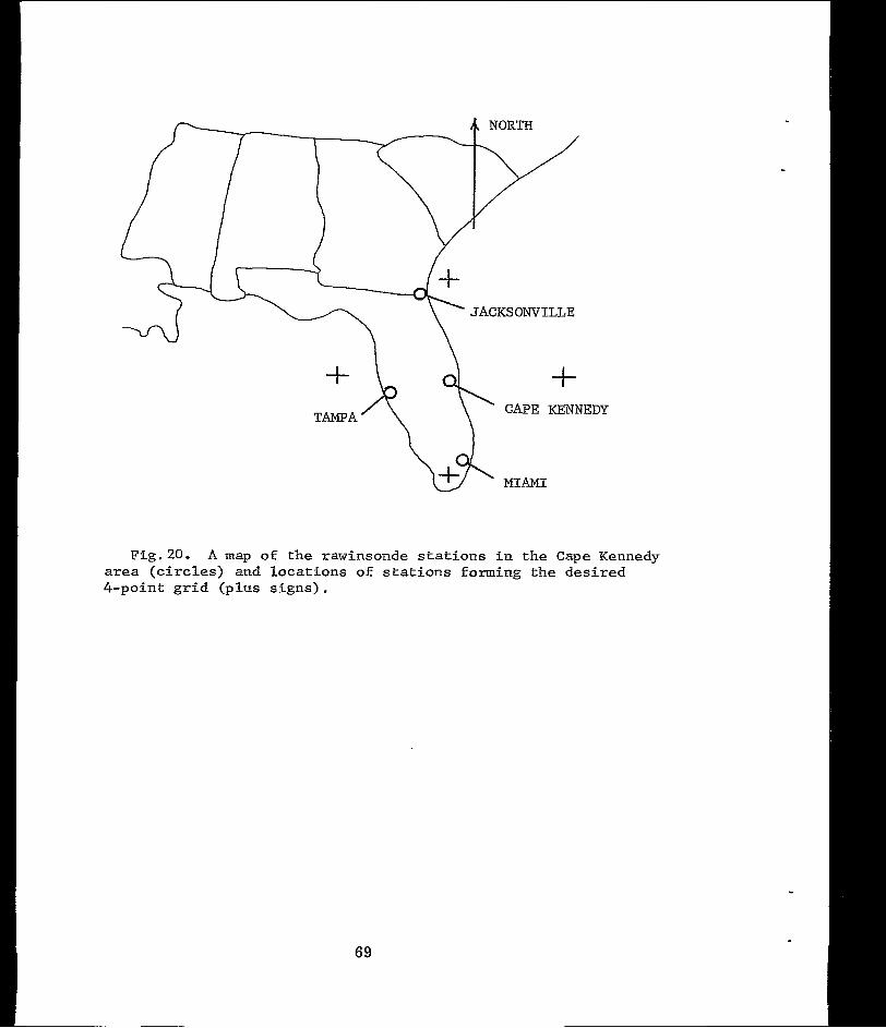
NORTH

MIAMI

Fig.20. A map of the rawinsonde s ta t ions in the Cape Kennedy area (circles) and loca t ions of s t a t i o n s forming the des i red 4-point grid (plus signs).

69

2. Forecasting Mean Virtual Temperature (Fv) or Thickness (Ah).

Equations 2 and 4 can be used to i l lustrate the importance of a

change in the gradient of the mean v i r tua l t empera ture (Tv) on the

geostrophic wind, Consider the case where the 1000-mb surface has

the same height over both Jacksonville and M i a m i . If the height of

the 700-mb surface at Jacksonvi l le i s 3100 m and Tv between the

1000- and 700-mb surfaces i s 4"C, and the corresponding values a t

M i a m i are 3125 m and 6"C, the zonal component of the geostrophic

wind would be approximately 6 m/sec. I f Tv a t Jacksonvi l le i s de-

creased by only 2OC, a very nominal change which could be realized

and the height of the 1000-mb surface remains unchanged, the re-

s u l t i n g change i n t h e h e i g h t o€ the 700-mb surface would be ap-

proximately 25 m. This increases the slope of the 700-mb surface

(also the magnitude of the pressure gradient force) by a fac tor o f

approximately 2 from i t s or ig ina l va lue and, hence, increases the

wind speed by the same f a c t o r , o r t o about 12 m/sec.

A change i n TV of t h i s magnitude easily could result from the

advection of temperature or from vert ical motion over a sho r t pe-

r iod of t i m e . If w e consider a ver t ica l ve loc i ty o f on ly l cm/sec

a t a l l a l t i t u d e s below the l eve l i n ques t ion and in the absence of

condensation, approximately a 2°C drop i n temperature would result:

due t o expansion over a period of 6 h r . Vertical motions of a few

centimeters per second over a la rge area are not uncommon, and thus

changes i n TV due t o vertical motion could resul t in a s i g n i f i c a n t

70

change in the geos t rophic wind over re la t ively short per iods of t i m e .

The t o t a l d e r i v a t i v e of Tv i n the x, y, p, t system may be

wr i t ten

The f i r s t t e r m on the right-hand side i s the local rate-of-change

of yv. The second term represents advection of where V i s the

average wind vector in the layer . The l a s t t e rm r ep resen t s ve r t i ca l

advection of 7 .

-f

V

V

A s noted by Panofsky (%. G.), i f T w e r e a conservative quan- -

V

t i t y , and ver t ical advect ion could be neglected, Eq. 8 becomes

which states that the local ra te-of-change of yv i s the r e su l t o f

advection of 7 . Normally, when there i s warm (cold) advection,

t h e a i r i s r i s i n g ( f a l l i n g ) and t h i s motion produces adiabatic

V

cooling (warming) and thus reduces the temperature change. Although

the error caused by neglecting vertical motion and changes i n

temperature fol lowing the a i r var ies in individual cases , the long-

term average i s tha t t he change i n r i s less than that expected

from advection alone (Panofsky, %. *.). V

The loca l t i m e rate-of-change of thickness as given by hori-

zontal advection only was invest igated. The isobaric advect ion of

thickness, -7. GP(Ah), i s numerically equal to -V a(Ah)/as, where

V i s t h e mean speed of the wind and a(Ah)/as i s the change of

thickness along the streamlines (Panofsky, %. G.). This re-

la t ionship w a s used to eva lua te t he i soba r i c advec t ion o f t h i ck -

ness from constant-pressure maps.

- -

NMC facsimile maps were re-analyzed as deemed appropriate and

used t o compute graphical ly the thickness pat terns and t h e mean

wind through and upstream from each s ta t ion. The mean wind speed,

V, f o r t h e s t a t i o n , w a s computed by averaging the wind speed both

along the s t reamline and between the two pressure surfaces. The

product of wind speed and the forecast period gives the approximate

dis tance t raveled by a parcel dur ing the forecast per iod. The fore-

c a s t of t he t h i ckness fo r t he s t a t ion i s made by reading the thick-

ness value from the analyzed map a t a point this dis tance upstream

along the contours.

-

The advection of thickness a t Cape Kennedy, Jacksonville, and

Miami between 500 and 700 mb, and between 500 and 300 mb, was com-

puted for a 12-hr period without respect to synopt ic condi t ions.

Figure21shows the resul ts of a comparison between the fo recas t

and measured change i n t h i c k n e s s f o r a l l t h r e e s t a t i o n s and fo r

both layers. The grouping of a l l t h e p o i n t s i n one f igure was

j u s t i f i ed because t he d i s t r ibu t ion of points for each s ta t ion and

layer showed no s ign i f i can t d i f f e rence from tha t of the composite.

The measured change i s plot ted a long the abscissa and the fo recas t

change along the ordinate. The so l id d iagonal l ine is where

72

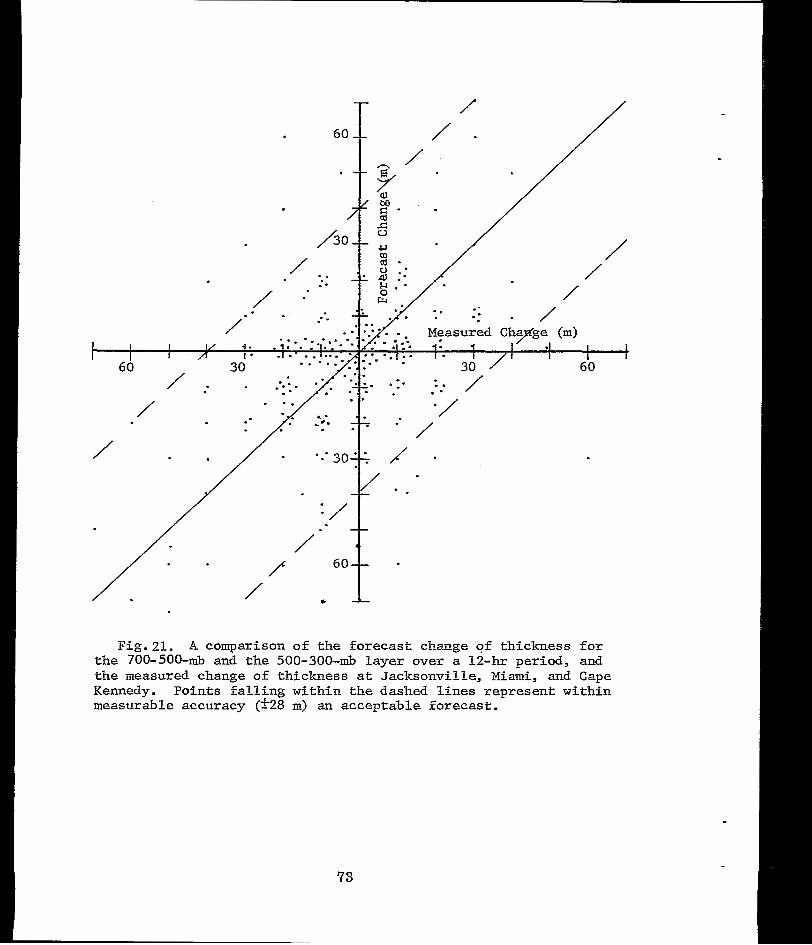
Fig.21. A comparison of the forecast change of thickness for the 700-5OGmb and the 500-300-mb layer over a 12-hr period, and the measured change of thickness at Jacksonville, Miami, and Cape Kennedy. Poin ts fa l l ing wi th in the dashed l ines represent wi th in measurable accuracy (-1.28 m) an acceptable forecast .

73

the points would f a l l i f a one-to-one relationship existed between

the measured and fo recas t change. For or ientat ion purposes , from

Eq. 4 a change of 60 m in th ickness of the 500- to 700-mb layer

corresponds to a 6°C change i n t h e TV. For the 500- t o 300-mb

layer , a change of 60 m in th ickness cor responds to a 4 ° C change

i n Tv.

Below 13 km, the RMS e r r o r i n p r e s s u r e measurements by the RW

system i s 1.50 mb.3 This means t h a t 67% of the measured da ta are

e i ther h igher o r lower than the true value by an amount equal t o o r

less than 1.50 mb. With t h i s i n mind, and using the hypsometric

r e l a t ionsh ip , we can ca lcu la te a corresponding RMS e r r o r of height

measurement. Since pressure decreases exponentially upwards from

the sur face , a 1.50-mb e r ro r i n p re s su re co r re sponds t o l a rge r

e r r o r s i n h e i g h t measurement a t t he h ighe r a l t i t udes . For example,

a t 700 mb i t is 18 m and a t 200 mb i t i s 48 m. For our purposes,

an average RMS e r r o r of 20 m was chosen and assumed t o apply a t

a l l l eve l s .

Since the thickness between two surfaces i s t h e d i f f e r e n c e i n

the i r he igh t s , t h i s t h i ckness va lue a l so has a c e r t a i n RMS e r r o r .

This RMS e r r o r of the thickness (0th) is r e l a t e d t o t h e EUG e r r o r

of the height of the upper surface (oU ) and the RMS e r r o r of the

AMR, 1963: Meteorological Handbook, Headquarters , A i r Force Missile Test Center , Patr ick AFB, Flor ida, 12 pp.

I - 74

lower surface (G,) by L

3 c)

5 t h = 4 5; f 5;

(Ueming, 1943). I f there are er rors o f 20 m a t each of t h e two

sur faces , the RMS e r r o r i n the th ickness would be about 28 m.

The dashed l ines in F ig .21 bracke t the RMS e r r o r in measurement

e 2 8 m) of thickness, so t h a t any p o i n t t h a t f a l l s w i t h i n these

limits represents an acceptable forecast . Of t h e 280 po in t s p lo t t ed

i n Fig. 21, 93% f a l l w i t h i n t h e s e l i m i t s .

As noted previously, the wind speed depends upon the gradien t

of the thickness and no t t he t h i ckness i t s e l f . The re fo re , fo recas t s

of the gradient of the thickness of a l aye r w e r e examined. A. mea-

s u r e of the gradient (north-south) of thickness i s obtained by

tak ing the d i f fe rence in the th ickness o f a l aye r between Jackson-

v i l l e and Miami, h e r e a f t e r r e f e r r e d t o as the "gradient".

O n the assumption that the local rate-of-change of thickness i s

a resu l t o f hor izonta l advec t ion a lone , the forecas t g rad ien ts w e r e

computed fo r bo th t he 500-700-mb and t h e 500-300-mb layers and t h e i r

measured and forecast changes compared. F igu re 22 i s a scatter dia-

gram of t h e r e s u l t s o f t h i s comparison. The measured change of t h e

grad ien t i s plot ted a long the abscissa and the forecast change of

the g rad ien t a long the o rd ina te . The diagonal lines i n t h e f i g u r e

have meanings similar to those i n Fig. 21. Equation 10 was used to

compute these l i m i t s us ing RMS e r ro r s ob ta ined fo r t he measurement

of thickness for Jacksonvi l le and Miami of 28 m, g iv ing for the RMS

7 5

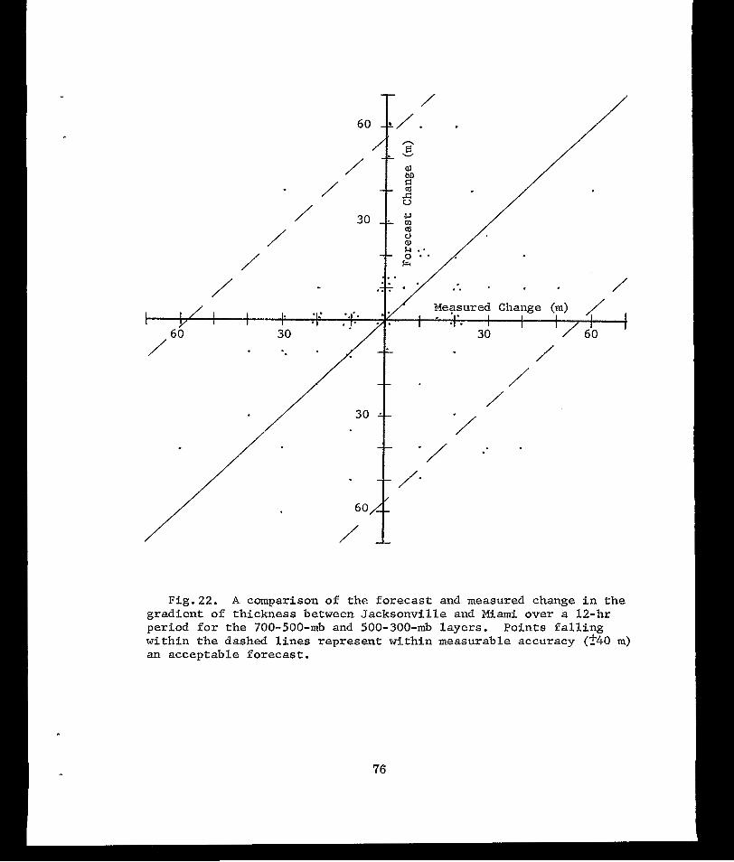
/ (d L)

/ / j.!, / /

.. /

I I I I I. . I . . * Y I I I

.I . I . I. I I I I I . . I I I I

Pleasured Change (m) / I

30 / 60

/ 4- / -

r n L'

Fig.22. A, comparison of the forecast and measured change i n t h e g rad ien t of thickness between Jacksonvi l le and Miami over a 12-hr p e r i o d f o r t h e 700-500-mb and 500-300-mb l a y e r s . P o i n t s f a l l i n g within the dashed l ines represent within measurable accuracy (240 m) an acceptab le forecas t .

76

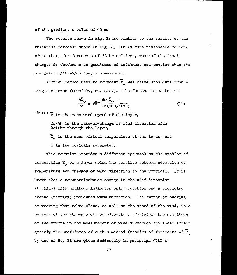
of the gradient a value of 40 m.

The r e s u l t s shown i n Fig. 22are s imilar to t h e r e s u l t s of t he

thickness forecast shown i n Fig. 21. It is thus reasonable t o con-

clude that , for forecasts of 12 hr and less, most -of the loca l

changes in th ickness o r g rad ien ts o f th ickness a re smal le r than the

precision with which they are measured.

Another method used to fo recas t 7 *was based upon d a t a from a V

s ing le

where :

s t a t i o n (Panofsky, =. G.). The forecast equation i s

aTv -2 acrr 77

a t ah(980) (180)

- " -fv - V

- V i s the mean wind speed of the layer ,

&/ah is the rate-of-change of wind direct ion with height through the layer,

T is the mean vir tual temperature of the l ayer , and

f i s the cor iol is parameter .

- V

This equation provides a different approach to t he problem of

forecas t ing r of a layer using the relation between advection of

temperature and changes of wind d i r e c t i o n i n t h e v e r t i c a l . It i s

known t h a t a counterclockwise change i n t h e wind d i r e a i o n

(backing) with a l t i tude indicates cold advect ion and a clockwise

change (veering) indicates warm advection. The amount of backing

or veer ing that takes place, as w e l l as the speed of t h e wind, is a

measure of the strength of the advection. Certainly the magnitude

of the e r rors i n the measurement of wind d i r e c t i o n and speed a f f e c t

greatly the usefulness of such a method ( r e s u l t s of forecasts of 7

by use of Eq. 11 are g iven ind i rec t ly in paragraph VI11 E).

V

V

77

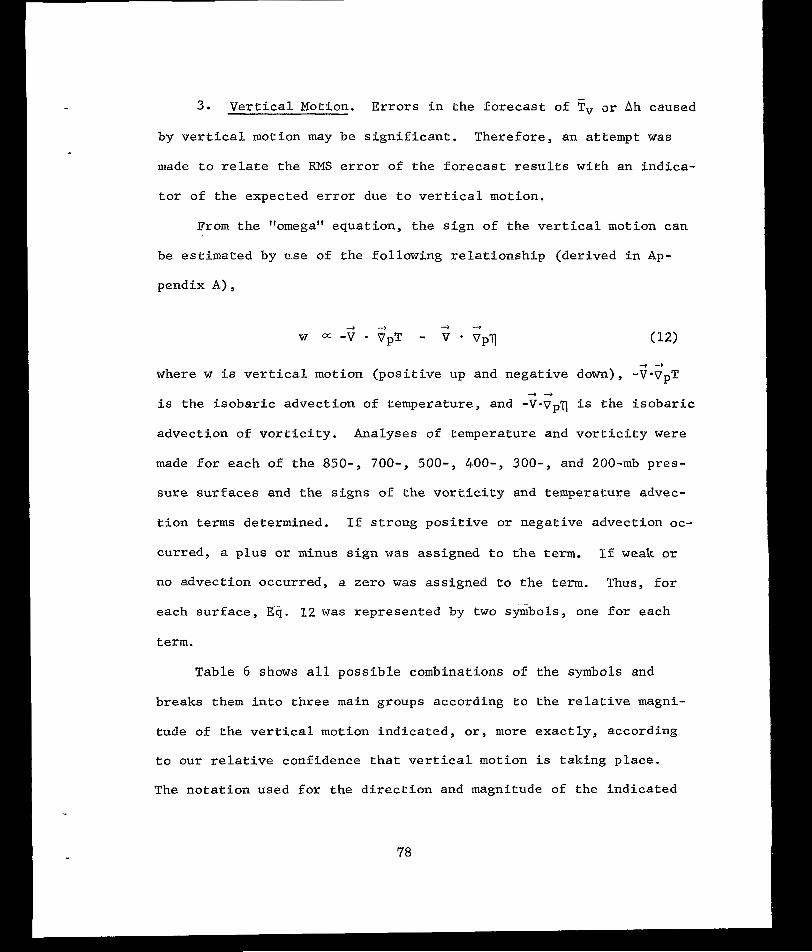
3 . Vertical Motion. Errors in the forecast of 5, or Ah caused

by vertical motion may be significant. Therefore, an attempt was

made to relate the RMS error of the forecast results with an indica-

tor of the expected error due to vertical motion.

From the "omega" equation, the sign of the vertical motion can

be estimated by use of the following relationship (derived in Ap-

pendix A),

where w is vertical motion (positive up and negative down), -V.vpT 4-9

is the isobaric advection of temperature, and -V.vpq is the isobaric

advection of vorticity. Analyses of temperature and vorticity were

4 -

made for each of the 850-, 700-, 500-, 400-, 300-, and 200-mb pres-

sure surfaces and the signs of the vorticity and temperature advec-

tion terms determined. If strong positive or negative advection oc-

curred, a plus or minus sign was assigned to the term. If weak or

no advection occurred, a zero was assigned to the term. Thus, for

each surface, Eq. 12 was represented by two symbols, one for each

term.

Table 6 shows all possible combinations of the symbols and

i breaks them into three main groups according to the relative magni-

tude of the vertical motion indicated, or, more exactly, according

to our relative confidence that vertical motion is taking place.

The notation used for the direction and magnitude of the indicated

78

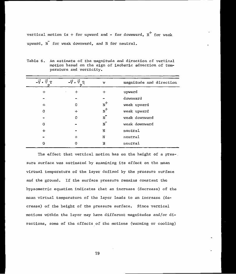
ver t ica l mot ion i s + f o r upward and - f o r downward, N f o r weak

upward, N- fo r weak downward, and N for neut ra l .

+

Table 6 . A n estimate of the magnitude and d i r ec t ion o f vertical motion based on the s ign of isobaric advect ion of tempera ture and v o r t i c i t y .

4-9

-V VDT W magnitude and d i r e c t i o n

+ +

0

+ 0

- + 0

+ - N+ N+ - N N N N N

-

upward

downward

weak upward

weak upward

weak downward

weak downward

neutral

neu t r a l

n e u t r a l

The e f f e c t t h a t vertical motion has on the height o f a p r e s - ,

sure sur face w a s estimated by examining i ts effect on t h e mean

vir tual temperature of the layer def ined by the p ressure sur face

and t h e ground. If the surface pressure remains constant the

hypsometr ic equat ion indicates that an increase (decrease) of the

mean v i r tua l t empera ture of the l ayer l eads t o an increase (de-

c rease) o f the he ight o f the p ressure sur face . S ince vertical

motions within the layer may have different magnitudes and/or di-

rec t ions , some of the e f fec ts o f the mot ions (warming or cool ing)

79

may o f f s e t one another. Therefore,. the height of the pressure

surface w i l l be affected by the in tegra ted ver t ica l mot ion below

the pressure surface.

The i n t eg ra t ed ve r t i ca l motion w a s es t imated using the re la-

tive magnitudes of the vertical motion indicated a t each of the

850-, 700-, 500-, 400-, 300-, and 200-mb surfaces. For example,

the in tegra ted ver t ica l mot ion below 850 mb w a s assumed t o be

represented by the motion indicated a t the 850-mb surface; the

integrated motion a t '500 mb w a s assumed to be a combination of the

motions indicated a t t h e 500-, 700-, and 850-mb surfaces . Further ,

i f t he i nd ica t ed mo t ions a t 850 and 700 mb are + and -, respec-

t ively, the integrated motion below 700 mb w a s assumed t o be repre-

sented by N. Similarly, i f t h e i n d i c a t e d v e r t i c a l m o t i o n s a t 500,

700, and 850 mb are +, N+, and N, respect ively, the integrated

v e r t i c a l motion below 500 mb was assumed t o be represented by N+. I n t h i s manner, an ind ica tor of t he i n t eg ra t ed ve r t i ca l motion,

h e r e a f t e r r e f e r r e d t o as v e r t l c a l motion, below each surface for

each case was obtained using the same nota t ion as descr ibed in

Table 6 .

In o rder to de te rmine the e f fec t o f ver t ica l mot ion on the

zonal wind speed a t Cape Kennedy, t he e f f ec t s o f ve r t i ca l motion

on the heights of the pressure surfaces a t Jacksonvi l le and Miami

were examined. I f t h e d i r e c t i o n and magnitude of the vertical

motion are ident ical a t Jacksonvi l le and M i a m i , then the s lope of

80

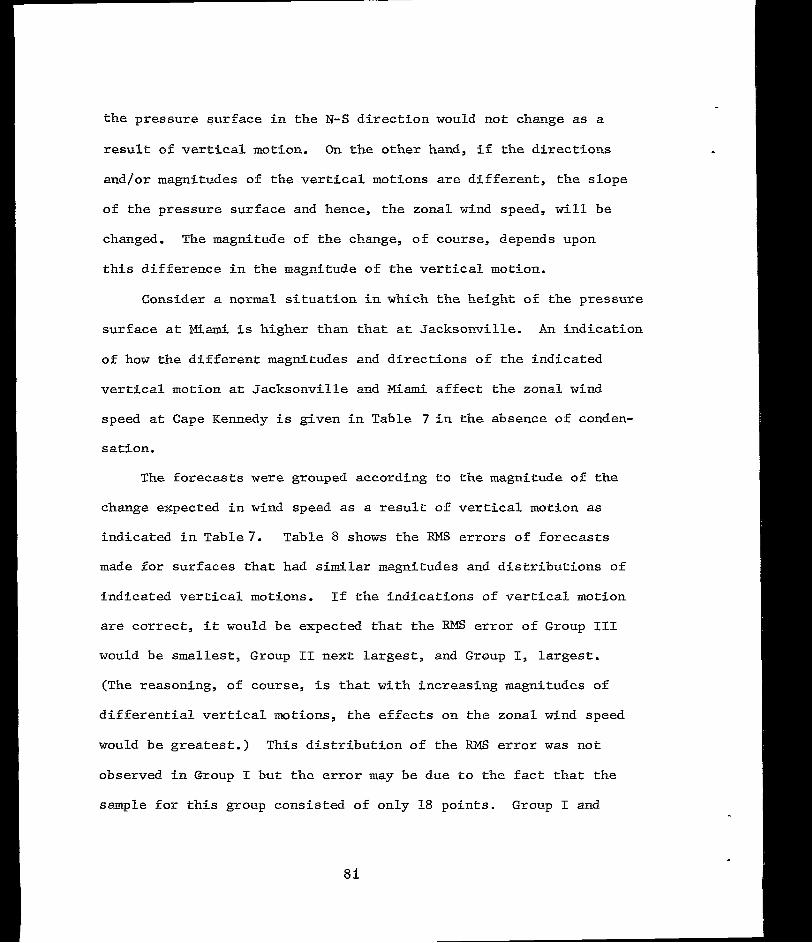
t he p re s su re su r f ace i n t he N-S d i r e c t i o n would not change as a

r e s u l t of v e r t i c a l motion. O n the other hand, i f the d i r e c t i o n s

and/or magnitudes of the vertical motions are d i f f e ren t , t he s lope

of the pressure surface and hence, the zonal wind speed, w i l l be

changed. The magnitude of the change, of course, depends upon

t h i s d i f f e r e n c e i n t h e magnitude of the vertical motion.

Consider a normal s i t u a t i o n i n which the he igh t of the p re s su re

sur face a t Miami i s higher than that a t Jacksonvi l le . An i nd ica t ion

of how the different magni tudes and d i r e c t i o n s of t he i nd ica t ed

ver t ica l mot ion a t Jacksonvi l le and Miami af fec t the zonal wind

speed a t Cape Kennedy i s g i v e n i n T a b l e 7 i n t h e a b s e n c e o f conden-

sa t ion .

The fo recas t s w e r e grouped according to the magnitude of the

change expected i n wind speed as a r e su l t o f ve r t i ca l mo t ion as

ind ica t ed i n Tab le7 . Tab le 8 shows the RMS e r rors o f forecas ts

made f o r s u r f a c e s t h a t had similar magnitudes and d i s t r ibu t ions o f

ind ica ted ver t ica l mot ions . I f the ind ica t ions o f ver t ica l mot ion

a re co r rec t , it would be expected that the RMS e r r o r of Group I11

would be smallest , Group I1 nex t l a rges t , and Group I, l a rges t .

(The reasoning, of course, i s that wi th increasing magni tudes of

d i f f e ren t i a l ve r t i ca l mo t ions , t he effects on the zonal wind speed

would be g rea tes t . ) This d i s t r i b u t i o n o f t h e Rplis e r r o r w a s not

observed i n Group I b u t t h e e r r o r may be due to the fact t h a t t h e

sample for th i s g roup cons is ted of only 18 poin ts . Group I and

81

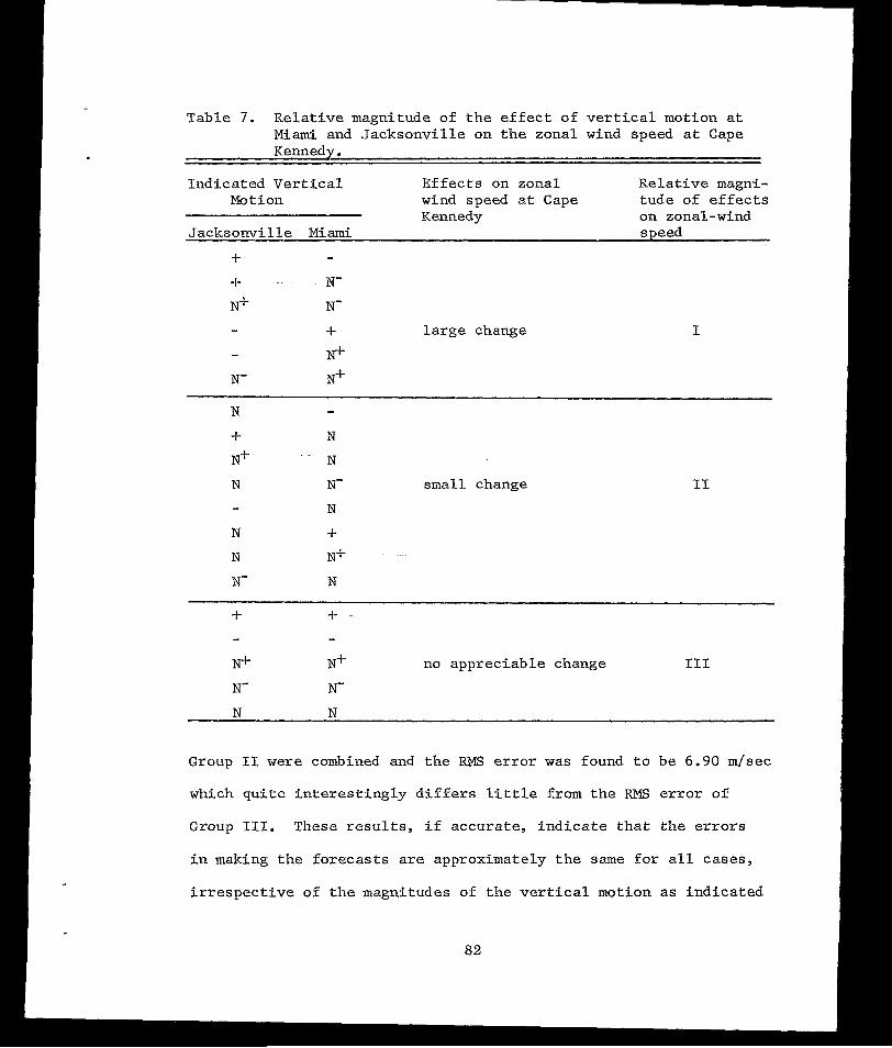
Indica ted Ver t ica l Ef fec ts on zonal Rela t ive magni- Motion wind speed a t Cape tude of effects

Kennedy on zonal-wind Jacksonvi l le M i a m i speed

+ + ~~ N'

-

N+ 'N- - + l a rge change I - N+

N' N+

N - + N N+ N

N N- - N N + N N+ N- N

~-

small change 11

+ +

N+ N+ no appreciable change 111

N' N"

N N

Group 11 were combined and the RMS e r r o r w a s found t o b e 6.90 m/sec

which q u i t e i n t e r e s t i n g l y d i f f e r s l i t t l e from t h e RMS e r r o r of

Group 111. These r e su l t s , i f a ccu ra t e , i nd ica t e t ha t t he e r ro r s

i n making the forecas ts are approximately the same f o r a l l cases,

i r r e s p e c t i v e of the magnitudes of t h e vertical motion as indicated

82

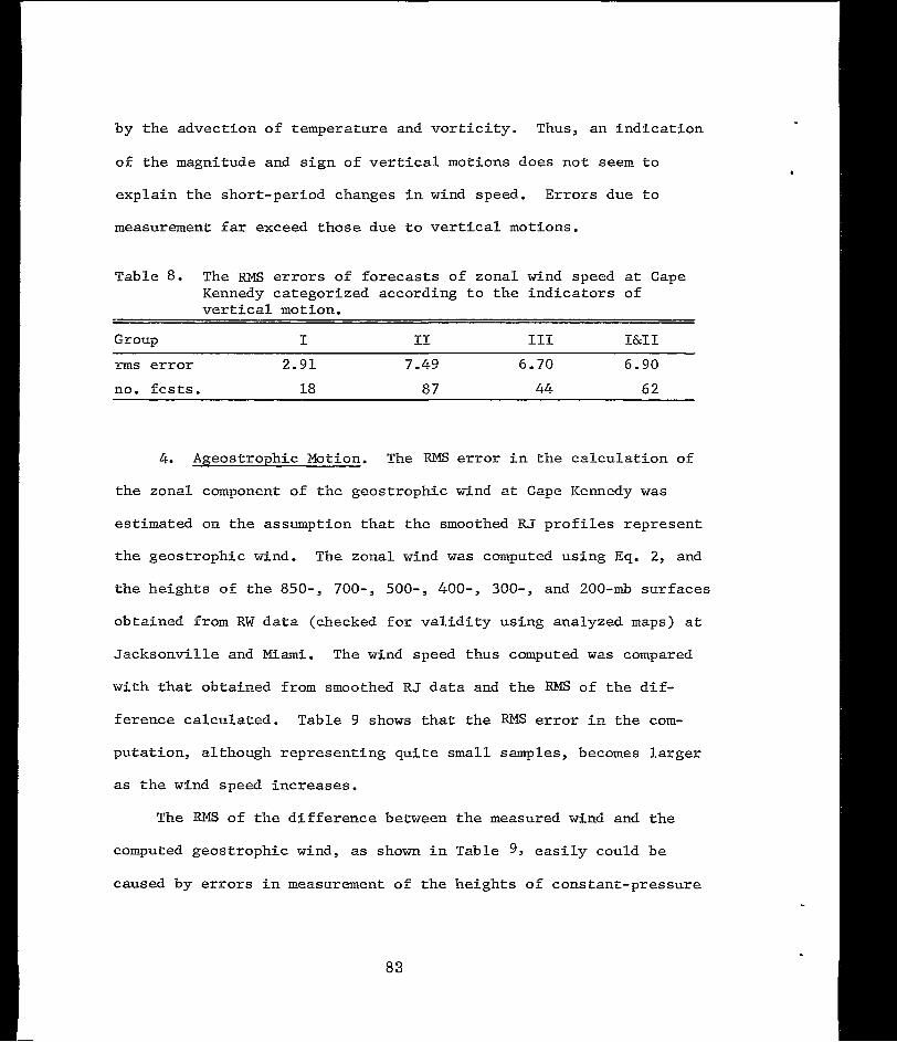
by the advection of temperature and v o r t i c i t y . Thus, an ind ica t ion

of the magnitude and sign of vertical motions does not seem to

explain the short-per iod changes in wind speed. Errors due to

measurement far exceed those due to vertical motions.

Table 8. The RMs errors of forecasts of zonal wind speed a t Cape Kennedy categorized according to t he i nd ica to r s of v e r t i c a l motion.

Group I 11 I11 I&II

rms e r r o r 2.91 7.49 6.70 6.90

no. f c s t s . 18 87 44 62

4 . Ageostrophic Motion. The RMS e r r o r i n t h e c a l c u l a t i o n of

the zonal component of the geostrophic wind a t Cape Kennedy was

estimated on the assumption that the smoothed R J p ro f i l e s r ep resen t

the geostrophic wind. The zonal wind w a s computed using Eq. 2, and

the heights of the 850-, 700-, 500-, 400- , 300-, and 200-mb surfaces

obtained from RW d a t a (checked for va l id i ty us ing ana lyzed maps) a t

Jacksonvi l le and Miami. The wind speed thus computed w a s compared

with that obtained from smoothed R J d a t a and t h e RMs of the d i f -

ference calculated. Table 9 shows t h a t t h e RMs e r r o r i n t h e com-

putat ion, a l though represent ing qui te s m a l l samples, becomes l a rge r

as the wind speed increases.

The RMS o f t he d i f f e rence between the measured wind and t h e

computed geostrophic wind, as shown i n Table 9 , easily could be

caused by e r r o r s i n measurement of the heights of constant-pressure

83

,

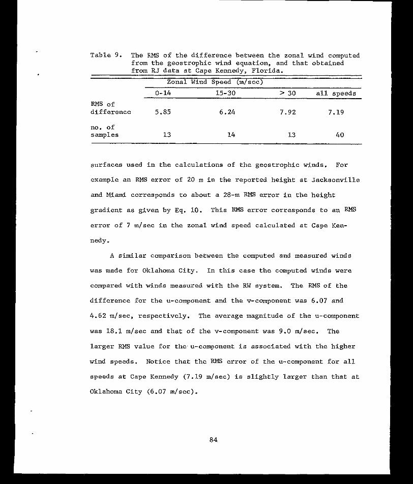
Table 9. The RMS of the difference between the zonal wind computed from the geostrophic wind equation, and that obtained from R J da t a a t Cape Kennedy, Flor ida.

Zonal Wind Speed (m/sec)

0- 14 15-30 > 30 a l l speeds

RMS of difference 5.85 6.24 7.92 7.19

no. of samples 13 14 13 40

surfaces used in the calculat ions of the geostrophic winds. For

example an RMS e r r o r of 20 m in the repor ted he ight a t Jacksonvi l le

and M i a m i corresponds to about a 28-m RMS e r r o r i n t h e h e i g h t

gradient as given by Eq. 10. This error corresponds to an RMs

error of 7 m/sec in t he zona l wind speed calculated a t Cape Ken-

nedy.

A similar comparison between the computed and measured winds

w a s made fo r Oklahoma City. In t h i s case t h e computed winds were

compared with winds measured with the RW system. The RMS of t he

d i f fe rence for the u-component and t h e v-component w a s 6.07 and

4.62 m/sec, respectively. The average magnitude of the u-component

w a s 18.1 m/sec and tha t o f the v-component was 9.0 m/sec. The

l a rge r RMS value for the.u-component i s associated with the higher

wind speeds. Not ice that the RMS e r ro r of t h e u-component f o r a l l

speeds a t Cape Kennedy (7.19 m/sec) i s s l igh t ly l a rge r t han t ha t a t

Oklahoma City (6.07 m/sec).

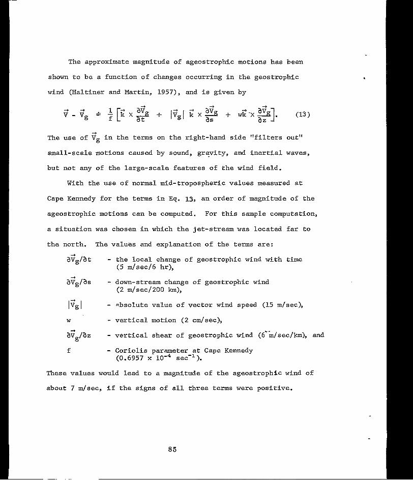
The approximate magnitude of ageostrophic motions has been

shown to be a function of changes occurring in the geostrophic

wind (Haltiner and Martin, 1957) , and is given by

The use of Vg in the terms on the right-hand side "filters out"

small-scale motions caused by sound, gravity, and inertial waves,

but not any of the large-scale features of the wind field.

+

With the use of normal mid-tropospheric values measured at

Cape Kennedy for the terms in Eq. 13, an order of magnitude of the

ageostrophic motions can be computed. For this sample computation,

a situation was chosen in which the jet-stream was located far to

the north. The values and explanation of the terms are:

aGg/at - the local change of geostrophic wind with time (5 m/sec/6 hr),

- down-stream change of geostrophic wind (2 m/sec/200 km),

1 3 8 I - xbsolute value of vector wind speed (15 m/sec),

W - vertical motion (2 cm/sec),

aGg/aZ - vertical shear of geostrophic wind (6&m/sec/km), and f - Coriolis parameter at Cape Kennedy

(0.6957 x IO'* see'').

These values would lead to a magnitude of the ageostrophlc wind of

about 7 m/sec, if the signs of a l l three terms were positive.

85

DeMandel and Scoggins &. s.) examined the small-scale

f luc tua t ions below 16 km as measured by the R J system. They ob-

served f luc tua t ions in wind speeds, a t times, i n excess of 5 m/sec,

some of which persisted for several hours. Quite probably, many

of these f luctuat ions consis ted of noise and turbulence caused by

random o s c i l l a t i o n s which were of the type f i l tered out because

of the assumpt ion tha t the rea l wind can be replaced by t h e geo-

s t rophic wind. Thus, t h e RMS e r r o r i n computing the geostrophic

wind i s equal to or greater than the expected magnitude of t h e

ageostrophic motions. For this reason, these motions cannot be

forecas t by the model.

86

E. U s e of t h e Model

Forecasts of the zonal wind w e r e made fo r s eve ra l ca ses i n

which t h e i n i t i a l RJ p ro f i l e o f a series coincided with the t i m e

of the RW data , 00 o r 12 GEE. From t h i s i n i t i a l t i m e , several

short-range forecasts w e r e made f o r times that coincided with

measured R J prof i les . The ' forecasts provided by t h e model were

compared with pers is tence.* Forecasts for the zonal wind speed

were made by use o f the forecas t model presented in paragraph VI11 C

with 850 mb as the base surface. Heights of this surface for the

forecast t imes w e r e interpolated between the 00 and 1 2 GMT data .

For example, i f R J p r o f i l e s w e r e measured a t 0010, 0215, 0345, and

0800 GI", t h e i n i t i a l t i m e would be assumed t o be 00 GMT and t h e

maps ana lyzed for th i s t i m e used t o make the fo recas t s . The 850-

mb heights a t Jacksonvi l le a t 00 and 12 GMT might be 1480 m and

1492 m, respect ively. The height w a s assumed to i nc rease l i nea r ly

during this per iod. The corresponding heights a t t he t h ree fo re -

cast t i m e s would be 1482, 1484, and 1488 m, respectively. This

i n t e rpo la t ion i s not exact, but i s be l i eved t o be be t t e r t han a

forecast based on information obtained a t and p r i o r t o 00 GMT.

With the graphical technique for advect ing the thickness pa t -

t e rns , a fo recas t w a s made for each of the 700-, 500- , 400- , 300- ,

and 200-mb pressure

w e r e separa ted in to

forecast per iod, P.

*A fo recas t of no

surfaces. These forecasts of the zonal wind

three g roups accord ing to the l ength o f the i r

The groups are P s 3 hr , 3 < P 5 6 hr , and

change.

87

6 < P 5 9 hr . Forecasts of a l l f ive surfaces within each group

were combined t o form a sample for each t i m e period, and the rms

e r ro r s of the forecasts provided by t h e model w e r e computed.

Forecasts a lso were made using Eq. 11 to advect the thickness

patterns. This i s ca l led the s ing le-s ta t ion method, s ince t he

local rate-.of-change of thickness (or T ) w a s evaluated with data

obtained from a s ing le s t a t ion . The forecas ts were separa ted in to

groups i n t h e same manner as the forecas ts made using the graphi-

c a l method, and the RMS e r ro r s were computed.

V

Figure 23 represents a comparison of the RMS errors of persis-

tence ( so l id l ine) , the g raphica l method (broken line) , and t h e

s ing le - s t a t ion method (dashed l i n e ) . The h o r i z o n t a l l i n e a t 13.2

m/sec represents the annual of the zonal wind speed (Vaughan,

1960). This vaLue i s fo r t he 7-km height which i s approximately

in the middle o f the reg ion for which the model was tes ted .

Thompson (1961) presented some in te res t ing resu l t s concern ing

the relative accuracy of numerical wind forecasts . H e found t h a t ,

in general, numerical techniques provide 24-hr forecasts with an

rms e r ro r 1/4 that of.climatology and l / 2 that of pers is tence. The

poin ts p lo t ted to the r igh t in F ig .23 *ere ca lcu la ted from t h i s

r e l a t ionsh ip and represent the RMS error of numerical forecasts

(N) and pers i s tence (P) based on the annual RMS e r ror o f the

zonal wind a t Cape Kennedy (13.2 m/sec). The poin ts p lo t ted a t

3, 6 , and 9 h r were computed from forecas ts made with the model.

88

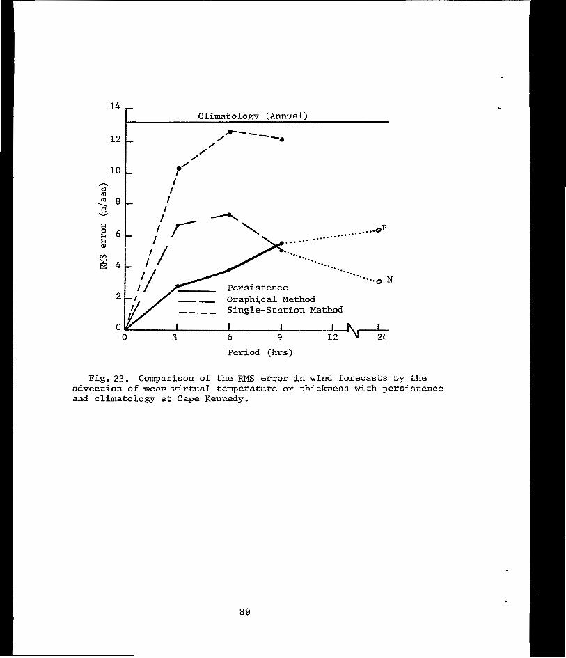
14 Climatology (Annual)

l2 t 0 i""

-0 0

/ 0

10 T'

. . . . . . ..op

-*. .. "..o N - - Graphical Method -___ Single-Station Method

I n- 0 3 6 9 12 - A 24

Period (hrs)

Fig.23. Comparison of the RMs error in wind forecasts by the advection of mean virtual temperature or thickness with persistence and climatology at Cape Kennedy.

89

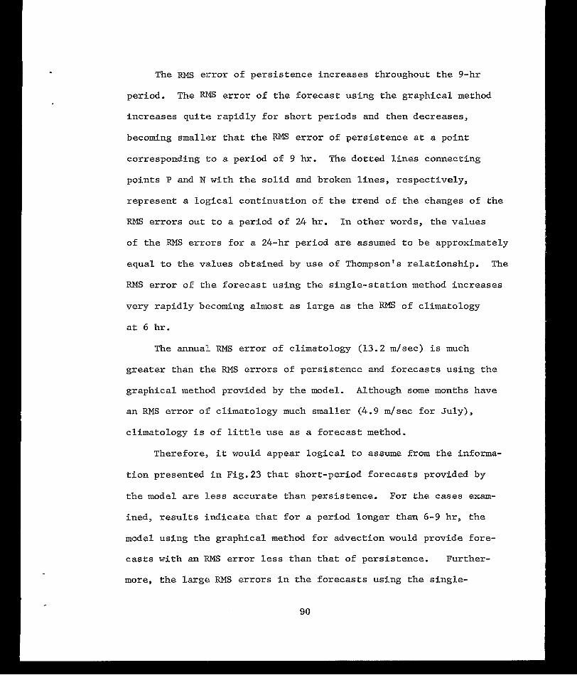
The EWS error of pers is tence increases throughout the 9-hr

period. The RMS error of the forecast us ing the graphical method

increases qu i te rap id ly for shor t per iods and then decreases,

becoming smaller t h a t t h e eMs e r r o r of p e r s i s t e n c e a t a point

corresponding to a period of 9 hr . The dot ted l ines connect ing

points P and N wi th t he so l id and broken l ines, respectively,

represent a logical cont inuat ion of the t rend of the changes of t he

RMS e r r o r s o u t t o a period of 24 hr . In other words, the values

of t he RMS e r r o r s f o r a 24-hr period are assumed t o be approximately

equal to the values obtained by use of Thompson's re la t ionship . The

RMS e r r o r of the forecas t us ing the s ing le-s ta t ion method increases

very rapidly becoming almost as large as the EMS of climatology

a t 6 hr .

The annual RMS error of climatology (13.2 m/sec) is much

grea te r than the RMS e r r o r s of pers i s tence and forecas ts us ing the

graphical method provided by t h e model. Although some months have

an RMS error of cl imatology much smaller (4.9 m/sec for Ju ly) ,

climatology i s of l i t t l e use as a forecas t method.

Therefore, i t would appear logical to assume from the informa-

t ion presented in Fig.23 that short-period forecasts provided by

t h e model are less accurate than persistence. For the cases exam-

i n e d , r e s u l t s i n d i c a t e t h a t f o r a period longer than 6-9 hr , the

model using the graphical method for advection would provide fore-

casts with an RMS e r r o r less than t ha t of persistence. Further-

more, t he l a rge RMS e r ro r s i n t he fo recas t s u s ing t he s ing le -

90

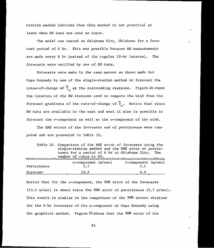
s t a t i o n method i n d i c a t e t h a t t h i s method i s no t p rac t i ca l a t

least when RW d a t a are used as input .

The model w a s t e s t ed a t Oklahoma City, Oklahoma f o r a fore-

cast per iod of 6 hr. This w a s possible because RW measurements

are made every 6 hr ins tead of the regular 12-hr in te rva l . The

fo recas t s w e r e v e r i f i e d by use of RW data .

Forecasts were made i n t h e same manner as those made f o r

Cape Kennedy by use o f the s ing le-s ta t ion method t o f o r e c a s t t h e

rates-of-change of T a t the surrounding stations. Figure24shows

the l oca t ion of t h e RW s ta t ions used to compute t h e wind from t h e

forecast gradients of the ra te-of-change of 7 . Not ice tha t s ince

RW d a t a are a v a i l a b l e t o t h e e a s t and w e s t it a l s o i s poss ib le to

- V

V

f o r e c a s t t h e v-component as w e l l as t h e u-component o f t he wind.

The RMS e r ro r s o f t he fo recas t s and of pers i s tence w e r e com-

puted and are presented i n Table 10.

Table 10. Comparison of the RMS e r r o r of forecas ts us ing the s ing le - s t a t ion method and t h e RMS er ror o f persis- t ence fo r a period of 6 h r a t Oklahoma City. The number of cases is 65.

u- component (m/ s ec) v-component (m/sec) Persistence 5.7 7.1

Forecast 12.5 9.2

Not ice tha t for the u-component, t h e EMS e r r o r of t he fo recas t s

(12.5 m / s e c ) is about t w i c e t h e RMS e r ror o f pers i s tence (5.7 m/sec).

Th i s r e su l t is similar t o t h e comparison of the errors obtained

for the 6 -hr forecas ts o f the u-component a t Cape Kennedy using

the g raph ica l method. Figure 23shows t h a t t h e e r r o r o f t h e

91

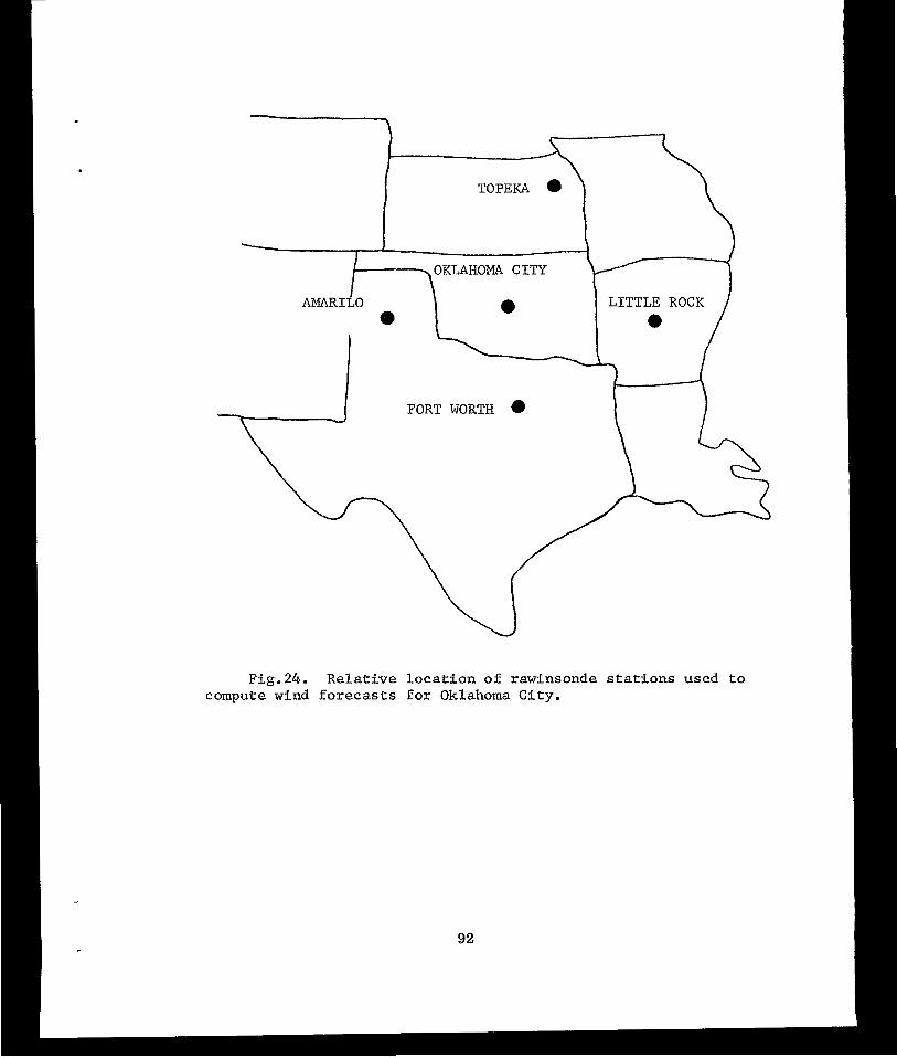
OKLAHOMA C I T Y

Fig.24. Relative location of rawinsonde stations used to compute wind forecasts for Oklahoma City.

92

f o r e c a s t f o r Cape Kennedy (7.5) m/sec) also i s about t w i c e the

RMS e r ro r due t o pe r s i s t ence (3.9 m/sec). Therefore , the relative

comparisons between the two sets of da ta are similar b u t t h e magni-

tudes of the RMS e r r o r s are no t t he same.

The increased magnitude of the REls e r r o r f o r t h e f o r e c a s t a t

Oklahoma Ci ty may b e a t t r i b u t e d t o t h e f a c t t h a t t h e s i n g l e -

s t a t i o n method i s much more dependent upon input data , especial ly

t h e e r r o r i n wind-direction measurements. Quite probably, the

analyzed maps used i n t h e o t h e r method d id e l imina te some of the

errors because of smoothing, hence the RMS e r r o r of t h e f o r e c a s t s

us ing the g raphica l method i s much smaller than those using the

s ing le - s t a t ion method.

93

LX. SUMMARY

Wind data provided by the R J system and thermodynamic da ta

provided by the RW system were used to inves t iga te re la t ionships

between motions of d i f f e ren t s ca l e , and t o tes t a simple model f o r

forecast ing the wi-nd p r o f i l e a t Cape Kennedy.

Small-scale or turbulent motions were defined as the d i f fe rence

between a smoothed p r o f i l e and t h e o r i g i n a l p r o f i l e measured by the

R J system, and a l s o as the difference between the smoothed s l a n t

range and the or iginal s lant range. Linear correlat ion coeff ic ients

between the small-scale motions defined by t h e d i f f e r e n t methods

were la rge i n magnitude and s t a t i s t i c a l l y s i g n i f i c a n t a t the 1%

level . This w a s i n t e rp re t ed t o mean tha t t he re was no s i g n i f i c a n t

difference between the small-scale motions defined by the d i f f e ren t

methods. For convenience, small-scale motions were defined as the

difference between a smooth p r o f i l e which approximates the RW sound-

ing and t h e o r i g i n a l p r o f i l e measured by the R J system.

The R J da t a were used to compute three of t he terms representing

the ra te of mechanical production of turbulent kinetic energy. Only

the terms involv ing the ver t ica l wind shear could be computed s ince

ho r i zon ta l wind shears were not avai lable . Of the three computed,

which involved the covariance between u, v, and w, mult ipl ied by the

ver t ica l wind shear, there did not appear to be any s i g n i f i c a n t d i f -

ferences. The magnitude of the terms were approximately the same

with some being negative and some pos i t i ve .

94

Scatter diagrams w e r e prepared with the RMS of the tu rbulen t

motions plot ted against vertical wind shear , the lapse rate of

temperature, and the Richardson number. A s a t i s f a c t o r y r e l a t i o n -

sh ip w a s not found between turbulence and any of the parameters

inves t iga ted . In addi t ion , scatter diagrams were prepared showing

relationshfps between the Richardson number computed ove r d i f f e ren t

a l t i t u d e i n t e r v a l s w i t h i n t h e same pro f i l e . It w a s shown t h a t wind

shears over smaller i n t e r v a l s i n p a r t i c u l a r i n f l u e n c e t h e v a l u e o f

the Richardson number grea t ly , and tha t t he re w a s scarcely any rela-

tionship between Richardson numbers computed over th in l ayers and

those over thick layers .

From the statistics of the small-scale motions, and considering

only those motions whose EUS value exceeds that due to error , the

frequency of measured turbulence agreed closely with the frequencies

given by Colson and Panofsky (1965) which w e r e computed from air-

c r a f t d a t a . Thus i t appears l ike ly tha t the J imsphere i s a good

turbulence sensor al though this remains to be proven by independent

measurements.

An a t t e m p t was made t o e s t a b l i s h r e l a t i o n s h i p s between parameters

determined from large-scale flow and thermodynamic da ta t aken f r o m

constant pressure maps, and t h e measured small-scale motions a t Cape

Kennedy, Flor ida. Parameters taken from t h e maps inc luded vo r t i c i ty ,

divergence, curvature, the advection of temperature and v o r t i c i t y ,

and o thers . No s ignif icant re la t ionships could be found. In addi-

t i on t o da t a t aken from maps, temporal cross-sections of changes i n

mean wind speed and small-scale motions taken from serial ascents

were analyzed. An attempt was made to explain the observed changes

from synopt$x-scale data. Again t he re were no c lear -cu t re la t ion-

ships found except that , generally, when cold-air advection w a s

taking place, the winds backed with height and when warm-air advec-

t i o n w a s taking place, the winds veered with height. Changes i n

wind speed, as w e l l as the RMS of the turbulent motions, did not

appear t o be r e l a t ed t o t he d i f f e ren t i a l advec t ion o f t empera tu re

o r t o t h e mean v e r t i c a l wind shear.

I n summary, th i s inves t iga t ion has shown tha t t he re are no

s imple relationships between a number of synoptic-scale parameters

and small-scale or turbulent motions. The processes involved are

so complicated that a more sophisticated approach is required.

A,model used t o f o r e c a s t t h e v e r t i c a l wind p r o f i l e was devel-

oped and t e s t ed . It was found that the accuracy of the forecast

model was dependent upon how w e l l the gradient of 5 was forecast .

Two methods were t r i e d t o f o r e c a s t 5 one using methods 05 single-

s t a t i o n a n a l y s i s , and the other a graphlcal technique that , i f ap-

p l i e d t o a numerical.scheme, would requi re a l a rge g r id network.

Both methods assumed changes i n r to take place through horizontal

advection alone. The graphical method proved t o be superior, al-

though neither provided short-period forecasts more accurate than

pers is tence for per iods less than 9 hr.

V

V’

V

96

It was found t h a t t h e e r r o r i n measurement was , i n most cases,

larger than the changes that took place. Also, the magnitude of

t h e errors precluded the use of vertical motion i n t h e model, s ince

t h e e f f e c t s of the e r rors w e r e l a rger than the e f f e c t s o f vertical

mot ion i t s e l f . It a l s o was concluded t h a t t h e magnitude of ageo-

strophic motions for the zonal wind speed i s of t h e same magnitude

as t h e e r r o r s i n computing t h e wind speed. Therefore, even i f

optimum height data could be obtained, similar e r r o r s i n t h e f o r e -

c a s t would occur as a r e s u l t of these random motions.

Although no attempt w a s made t o estimate t h e e r r o r d u e t o t h e

finite-difference approximation used, it i s assumed t o b e small i n

comparison t o the o ther e r rors . ?h is i s s u b s t a n t i a t e d p a r t i a l l y

by t h e f a c t t h a t the rms er ror o f the d i f fe rence be tween the compu-

ted (using f ini te-difference approximation for s lope of pressure

sur face) and measured wind speeds i s similar to t he va lues g iven

for the magnitude of ageostrophic motion and the magnitude due t o

e r r o r s i n h e i g h t measurement.

It seems tha t fo recas t s fo r pe r iods less than 9 hr cannot be

made by t h e model with an accuracy bet ter than pers is tence. How-

ever, it does s e e m tha t fo r pe r iods g rea t e r t han 9 h r , t he fo re -

c a s t model could prove to be u se fu l .

97

REFERENCES

Blackburn, James H., Jr., 1969: "AStudy of Clear-Air Turbulence From Detailed Wind Profiles Over Cape Kennedy, Florida", M.S. Thesis, Department o f Meteorology, Texas A&M University, 42 PP*

Blackburn, Robert R. , 1968: "Responses of the Saturn V Space Vehicle to Inflight Wind Profiles", Proceedings of the Third National Conference on Aerospace Meteorology, American Meteorological Society, 327-336.

Colson, D. , and H. A. Panofsky, 1965: "An Index of Clear Air Turbulence",. Quart. Jour. Roy. Met. SOC., 91, 507-513.

Daniels, Glenn E., James R. Scoggins, and Orvel E. Smith, 1966: "Terrestrial Environment (Climatic) Criteria Guidelines for Use in Space Vehicle Development, 1966 Revision", NASA Techni- cal Memorandum, TM X-53328.

DeMandel, R. E., and James R. Scoggins, 1967: "Mesoscale Wave Motions as Revealed by Improved Wind Profile Measurements", Jour. Appl. Met., 6(4), 617-620.

Deming, Edward W. , 1943: Statistical Adjustment of Data, John Wiley and. Sons , Inc. , New York.

Eckstrom, Clinton V., 1965: "Theoretical Study and Engineering Development of Jimsphere Wind Sensor", Final Report, NASA Contract No. NAS8-11158, 78 pp.

Endlich, R. M., and J. W. Davies, 1967: "The Feasibility of Measuring Turbulence in the Free Atmosphere from Rising Bal- loons Tracked by FPS-16 Radar", Jour. Appl. Met. , 6 (1) , 43-47.

Endlich, R. M., R. C. Singleton, K. A. Drexhage, and R. L. Mancuso, 1969: "Studies o f Vertical Wind,Profiles at Cape Kennedy, Florida", NASA. CR-61263, Contract NAS8-21148, Stanford Research Institute, Menlo Park, California, 88 pp.

Hadeen, K. D. , 1966: A Meteorological Model for Forecasting the I t

Wind-Profile Between 1.0 and 18.0 Kilometers". Ph.D. Disserta- tion, Texas A&M University, 85 pp.

Kaltiner, G. J. and F. L. Martin, 1957: Dynamical and Physical Meteorolopy, McGraw-Hi11 Book Company, Znc., New York, 470 pp.

98

Hess, S. L. 1959: Introduction to Theoretical Meteorology, Henry Holt and Company, New York, 362 pp.

Leviton, Robert, 1962: IIA Detailed Wind Profile SounCing Tech- nique", Air Force Surveys in Geophysics, (140) , AFCRL, Bedford, Mass., 187-195.

Lumley, J. L., and H. A.- PTnofsky, 1964: Structure of Atmospheric ~~~ -

Turbulence, John Wiley and Sons, New York.

Panofsky, H. A. , 1965: Introduction to Dynamic Meteorolopy, The Pennsylvania State University, University Park, Pennsylvania, 243 pp.

Petterssen, S., 1956: Weather Analysis and Forecasting, McGraw- Hill Book Company, Inc., New York, 428 pp.

Reiter, E. R., 1963: "Nature and Observation of High Level Turbu- lence Especially in Clear Air", Technical Paper No. 41, Depart- ment of Atmospheric Science, Colorado State University, Fort Collins, 39 pp.

Reiter, E. R., and P. F. Lester, 1967: 'The Dependence of the Richardson Number on Scale Length", Atmospheric Sciences Paper No. 111, Colorado State University, Fort Collins, Colorado, 39 PP-

Rogers, .R. R., and H. G. Camnitz, 1965: "Project Baldy -- An Inves- tigation of Aerodynamically-Induced Balloon Motions", Final Report, NASA Contract No. NAS8-11140, 80 pp.

Ryan, R. S., J. R. Scoggins, and A. King, 1967: "Use of Wind Shears in the Design of Aerospace Vehicles", Jour. Spacecraft and Rockets, 4(11) , 1526-1532.

Sawyer, J. S., 1961: "Quasi-Periodic Wind Variations with Height in the Lower Stratosphere", Quar. Jour. Roy. Met. SOC. , 87(371), 24 PP-

Scoggins, James R., and William W. Vaughan, 1964: "Problems of Atmospheric Wind Inputs for fissile and Space Vehicle Design", J. Spacecraft, 1(2), 181-184.

Scoggins, James R. 1964: "Aerodynamics of Spherical Balloon Wind Sensors", Journal of Geop. Res., 69(4), 591-598.

99

Scoggins, James R., 1965: "Spherical Balloon Wind Sensor Behavior", Jour. o f Appl. Met., 4(1), 139-145.

, 1967: "Sphere Behavior and the Measurement of Wind Profiiesl', NASA. Technical Note TN D-3994, 53 pp.

Scoggins, James R. and Manuel Armendariz, 1969: "On the Measure- ment of Winds by the AN/FPS-16 Radar/Spherical Balloon Method", Jour. Appl.. Met. , 8(3), 449-452.

Susko, Michael and William W. Vaughan, 1968: "Accuracy of Wind Data Obtained by Tracking a Jimsphere Wind Sensor Simulta- neously With Two FPS-16 Radars", NASA Technical Memorandum, TM X-53752, 43 pp.

Sutton, 0. G., 1953: Micrometeorology, McGraw-Hi11 Book Company, 15 2- 153.

Thompson, P. D., 1961: Numerical Weather Analysis and Prediction. MacMillan Company, New York, 170 pp.

Vaughan, W. W., 1960: tlInterlevel and Intralevel Correlations of Wind Components for Six Geographical Locations", NASA TN D-561, 92 PP-

, 1968: "New Wind-Monitoring System Protects R&D Launches", Astronautics and Aeronautics, 6(12), 49-57.

Weinstein, A . I., E. R. Reiter and J. R. Scoggins: "Meso-scale Structure of 11-20 km Windsft, Jour. Appl. Met., 5(1), 49-57.

Zartarian, Garabed and John H. .Thompson, 1968: "Validity of Detailed Balloon Soundings in Booster Vehicle Design", Scientific Report No. 1, Contract No. F19-628-C-0205, AFCRL-68-0606.

100

APPENDIX A

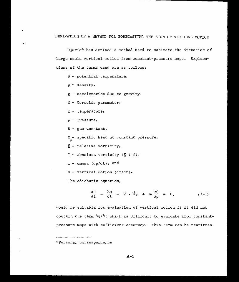
DERIVATION OF A METHOD FOR FORECASTING THE SIGN OF VERTICAL mTIOEJ

Djuric* has derived a method used to estimate the direction of

large-scale vertical motion from constant-pressure maps. Explana-

tions of the terms used are as follows:

9 - potential temperature, p - density, g - acceleration due to gravity, f - Coriolis parameterr T - temperature, p - pressure, R - gas constant, C - specific heat at constant pressure, 5 - relative vorticity, 7 - absolute vorticity (5 + f), w - omega (dp/dt), and w - vertical motion (dz/dt) The adiabatic equation,

P

de - - - I TT - na I E n ae - 4 ae

would be suitable for evaluation of vertical motion if it did not

contain the term %/at which is difficult t o evaluate from constant-

pressure maps with sufficient accuracy. This term can be rewritten

:';Personal correspondence I

and eliminated by use o f t he vo r t i c i ty equa t ion .

From t h e d e f i n i t i o n of 8,

TZ

8 = T [TI , where K = - c y P

1000" R

and the equat ion of state,

w e can write

Using the hydrostat ic equat ion,

and Eq. A-2y w e can wri te

where

Di f f e ren t i a t ing Eq. A-3 with respec t t o t i m e gives

which, when s u b s t i t u t e d i n t o Eq. A-I., gives

z [ - j a a - - c ~ . ~ ~ ~ + = 0 , 4 4

A- 3

where ae ap

5 = - c-

is a measure of the stability, positive in a stable atmosphere.

An approximate form o f the vorticity equation may be written

(Thompson, 1961)

which neglects small-magnitude terms such as vertical advection

of vorticity;

Taking the partial derivative of Eq. A-5 with respect to p

and the Laplacian of Eq. A-4, we can eliminate the time derivative

term (?aa"z/atap) by subtracting one equation from the other.

Rearranging terms gives the omega equation,

Under ordinary conditions a and p/g are positive. Then

Eq. A-6 is an elliptical equation and has solutions if boundary

conditions are provided on all boundaries of the region considered.

The simplest condition, w = 0 , on the boundaries is satisfactory if

the boundaries are far from the area of interest.

The left side of Eq. G-6 behaves like a three-dimensional

Laplacian of omega (w). Also, the constants on the right-hand side

are irrelevant in the process of a qualitative estimation of omega.

A-4

Therefore, the proportionality may be written

For many meteorological functions which vary around zero, the

proportionality holds that the sign of the two- or three-dimensional

Laplacian of a quantity evaluated at a point is opposite that of the

quantity at that point; thus,

Since vorticity advection usually increases with height, we

can write

Thus, Eq. A-7 can be rewritten

W a +

or, since w a -w,

Thus upward (downward) motion is followed by two main circum-

stances: (1) positive (negative) vorticity advection and (2) warm

(cold) air advection. I n most cases, if both terms are positive,

upward motion would result. Conversely, if both cerms are nega-

tive, downward motion would usually take place. When the terms

A- 5

are of oppos

motion but d

is lessened.

Thompson, P. MacMill

,ite sign, this method

.oes indicate that the

REFERENCE FOR

D., 1961: Numerical .an Company, New York,

does not give the direction of

probability of vertical motion

ASPEXWIIX A

Weather Analysis and Prediction, 170 pp.

APPENDIX B

k STUDY O F CLEAR-AIR-TURBULENCE FROM DETAILED WIND PROFILES OVER CAPE KENNEDY, FLORIDA

A T h e s i s

by

James H a r v e y B l a c k b u r n , Jr.

C a p t a i n

U n i t e d S t a t e s A i r Force

S u b m i t t e d t o the G r a d u a t e C o l l e g e o f the

T e x a s A&M U n i v e r s i t y i n partial f u l f i l l m e n t of the r e q u i r e m e n t s for the degree of

MASTER OF SCIENCE

May 1969

Major S u b j e c t : Meteorology

ABSTUCT

A Study of Clear-Air Turbulence from Detailed Wind P r o f i l e s Over

Cape Kennedy, Florida.

James H. Blackburn, Jr., B.S., Texas B&M University

Directed by: D r . James R. Scoggins

Clear-air turbulence (CAT) is invest igated by the analysis of

d e t a i l e d wind p r o f i l e s from FPS-16 radar/Jimsphere balloons and of

measurements of temperature from rawinsondes., Relationships were

established between CAT, def ined f rom the detai led wind p r o f i l e s ,

and mean meteorological parameters. The r e s u l t s of t h i s i n v e s t i -

gation show t h a t l a r g e vertical wind shear is necessary, but not

suff ic ient , for the occurrence of GAT. CAT occurred i n r e l a t i v e l y

s t a b l e and shallow ( S 1000 m) v e r t i c a l l a y e r s of the atmosphere from

5 t o 14 km i n the presence of large wind shear. These conditions

are f avorab le fo r t he ex i s t ence of unstable shear-gravi ty waves. To

p r e d i c t CAT, t hese s t ab le l aye r s w i th l a rge wind shear must be

fo recas t .

The s t a t i s t i c s relative to the frequency of occurTence of CAT

agree w e l l with previous data obtained by other methods. CAT w a s

observed approximately 2 to 5% of the total . number of observations,

depending on thickness of the layer. The FPS-16 radar/Jirnsphere

balloon system, because of i ts over-all cost advantage, accuracy,

and f l e x i b i l i t y , p r o v i d e s what appears t o be the best system

a v a i l a b l e f o r tlie c o l l e c t i o n oE CAT data.

B-iii

ACKNOWLEDGMENTS

The author 's graduate program w a s sponsored and financed by

the United States Air Force under the Air F o r c e I n s t i t u t e of

Technology program.

P a r t i a l f i n a n c i a l a i d was furnished by the Texas A&M Research

Foundation, Texas A&M University.

The d a t a u s e d i n t h i s i n v e s t i g a t i o n were kindly provided by

the Aerospace Environment Division, NASA Marshall Space Flight

Center, Huntsvil le, Alabama. My sincere appreciat ion i s extended

to th i s o rganiza t ion .

My g r a t i t u d e i s extended to D r . George L. Huebner, Jr., D r .

Archie R. Burgess, and D r . Vance E. Moyer f o r t h e i r encouragement

and a s s i s t a n c e i n t h e f i n a l p r e p a r a t i o n of the manuscript. I a l so

s incere ly apprec ia te the g race of Miss Lynda Su l ik who p a t i e n t l y

typed the manuscript . My most s incere apprec ia t ion is expressed to Capt. Robert L.

C r o f t f o r h i s a s s i s t a n c e i n t h e computer programming of the data,

and to D r . James R. Scoggins for his guidance, encourazement, and

t i m e . The deepest expression of g r a t i t u d e i s due my wife, "Charlie",

and our chi ldren, T e r i Lyn and Craig, f o r t h e i r p a t i e n c e and under-

standing throughout my graduate program.

TABLE OF CONTENTS

ABS.CT ................................................... ACKNOWLEDGMENTS ............................................ LIST OF FIGURES ............................................ LIST OF TABLES ............................................. SECTION 1 INTRODUCTION .................................

a . B a c k g r o u n d ............................ b . Purpose and M e t h o d of this Study ......

Page

B- iii

B- i v

B - v i i

B - v i i i

B-1

B- 1

B-6

SECTION 2 MEASUREMENT SYSTEpls AND DESCRIPTION OF TKF DATA .........................................

a . The FPS-16 R a d a r / J i m s p h e r e S y s t e m ..... b . R a w i n s o n d e System .....................

SECTION 3 MEASURFMENTS AND OBSERVATIONS OF CAT ......... SECTION 4 ANALYSIS OF THE DATA .........................

a . Preparation of the D a t a €or C o m p u t e r Processing ............................

b . Selective G r o u p i n g of the D a t a ........ c . C o m p u t a t i o n s P e r f o r m e d ................

SECTION 5 RESULTS ...................................... a . E m p i r i c a l Frequencies of CAT .......... b . R e l a t i o n s h i p s B e t w e e n CAT and Selected

M e t e o r o l o g i c a l P a r a m e t e r s ............. SECTION 6

SECTION 7

FORECASTING OF CAT ........................... CONCLUSIONS AND RECOIWENDATIONS ..............

B-10

B-10

B-11

B-11

B-13

B-13

B-13

B-14

B-16

B-16

B-18

B-35

3-36

B-v

Page

a . Conclusions .......................... B-36

b . Recommendations. ..................... B-37

.FERENCES ................................................. 3-39

VLTA ....................................................... 3-42

B-vi

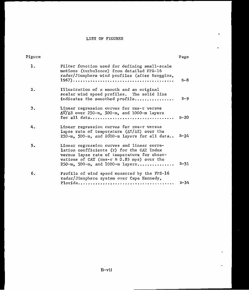
Figure

LIST OF FIGURES

, Page

F i l t e r f u n c t i o n u s e d f o r d e f i n i n g small-scale motions ( turbulence) f rom detai led FPS-16 radar/J imsphere wind prof i les (af ter Scoggins , 1967) ......................................... B-8

1.

2.

3.

4.

5 .

6.

I l l u s t r a t i o n of a smooth and an o r i g i n a l s c a l a r wind speed profiles. The s o l i d l i n e ind ica t e s t he smoothed p r o f i l e . . .............. B-9

Linear regression curves f o r rms-r versus Av/AZ over 250-m, 500-m, and 1000-m l aye r s for a l l data. . ................................ B-20

Linear regression curves €or rms-r versus l apse rate of temperature (AT/AZ) over the 250-m, 500-m, and 1600-m l a y e r s f o r a l l data . . B-24

Linear regression curves and l inear corre- l a r ion coe f f i c i en t s ( r ) f o r the CAT Index versus lapse rate of temperature €or observa t ions of CAT (rms-r 2 0.85 mps) over the 250-m, 500-111, and 1000-rn l a y e r s ............... B - 3 1

P r o f i l e of wind speed measured by the FPS-16 radar/.Jimsphere system over Cape Kennedy, Flor ida. . . . . . . . . . . . . . . . . . . . . . . . . . . ............ B-34

B-vii

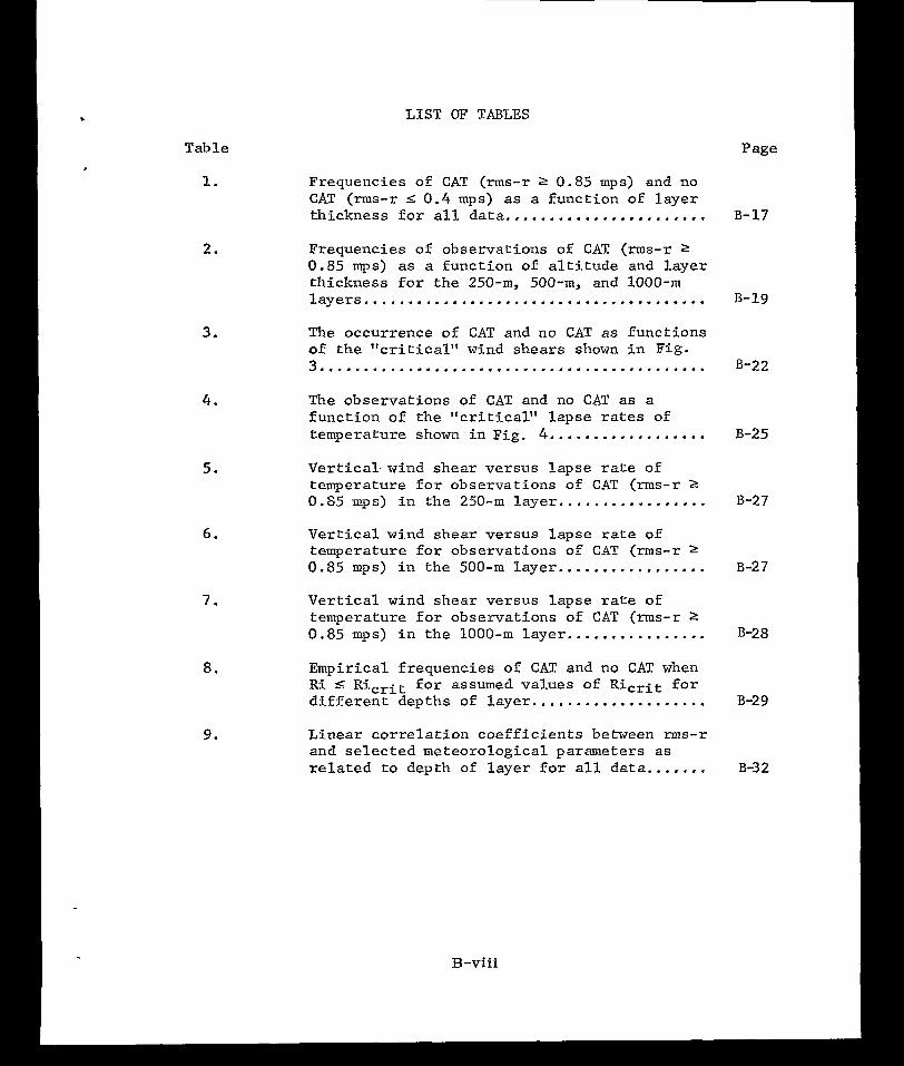
3.

4.

5 .

6.

7.

8 .

9.

LIST OF TABLES

Table

1. Frequencies of CAT (rms-r 2 0.85 mps) and no CAT (rms-r I, 0.4 mps) as a func t ion of l aye r th ickness for a l l data . , . . . . . . . . . . . . . . . . . . . . .

2. Frequencies of observations of CAT (rms-r 2 0.85 mps) as a funct ion of a l t i t u d e and l a y e r th ickness for the 250-m, 500-m, and 1000-m l aye r s ....................................... The occurrence of CAT and no CAT as func t ions o f t he " c r i t i ca l " wind shears shown i n Fig. 3 . . . . . . . . . . . . . . . . . . . . . . . . . . . . . . .............. The observat ions of CAT and no CAT as a func t ion o f t he " c r i t i ca l " l apse r a t e s of temperature shown in F ig . 4..................

Vert ical .wind shear versus lapse rate of temperature for observations of CAT (rms-r 2 0.65 mps) i n t he 250-m layer . . ............... Ver t i ca l wind shear versus l apse rate of temperature for observatdons of CAT (nns-r 2 0.85 mps) i n t h e 500-m l aye r ................. V e r t i c a l wind shear versus l apse ra te of temperature €or observations of CAT (nns-r 2 0.85 mps) i n t h e 1000-m layer ................ Empir ical frequencies of CAT and no CAT when R i S R i c r i t f o r assumed values of Ric, i t f o r d i f fe ren t depths of layer .................... Linea r co r re l a t ion coe f f i c i en t s between rms-r and selected meteorological parameters as r e l a t ed t o dep th of l a y e r f o r a l l data . ......

Page

B- 17

B-19

B-22

B-25

B-27

B-27

B-28

B-2 9

B-3 2

I. INTRODUCTION

a. Background. Clear-air turbulence (CAT) i s defined as any

turbulence above 6 7sm MSL not associated with clouds (Clem, 1957).

CAT usua l ly is assoc ia ted wi th s t rong hor izonta l and vertical wind

shears and/or temperature gradients . The i n t e n s i t y and p robab i l i t y

of occurrence of CAT are higher over land than over water, and much

higher over mountains than over plains (Reiter, 1963). Winter i s

the m o s t favorable season for the occurrence of CAT. In winter ,

moderate and s t ronger CAT occurs less than 5% of f l i gh t - t ime

(Endlich and Mancuso, 1965).

CAT i s of considerable importance to t he en t i r e av i a t ion e s t ab -

l ishment. Aircraft manufacturers inust design a i r f rzmes s t rong

enough to withstand near extreme conditions of atmospheric turbu-

lence. The a i r l i n e s and the mi l i ta ry agencies are i n t e r e s t e d i n

CAT because i t a f f e c t s t h e s a f e t y and comfort of passengers and crews.

The government agencies responsible for rhe direction, control, and

safe ty o f aircraft must consider CAT. Sc ien t i s t s suppor t ing the

av ia t ion es tab l i shment have an in te res t in CAT f o r a l l the p rev ious ly

mentioned reasons, and also because CAT is a phenomenon of our

environment that i s not clearly understood. Because of the increased

range and speed of newer a i r c r a f t , CAT has become a problem of

pronounced s ign i f icance in re la t ion to aircraft operat ions on a

The c i t a t i o n s on the fol lowing pages fol low the s tyle of the J O U L L ~ ~ of A p p l i ~ d Keteo-rology.

B-i

world-wide basis.

CAT i s found to be less intense than turbulence encountered in

thunderstorms (Foltz, 1967), but CAT has been known to cause passen-

g e r i n j u r i e s and l o s s of a i r c r a f t c o n t r o l , I n rare instances, CAT

has been found to be the prime cause of airframe damage (Reiter,

g . c i t . ) . CAT must be considered as dangerous as turbulence

encountered i n a thunderstorm because, i n most cases, i t occurs

with no v i s i b l e warning.

The present techniques of forecasting CAT f o r a i r c r a f t o p e r -

a t i o n s are based on the use of synoptic-scale data (> 500 km

hor izonta l d i s tance) . This scale i s inadequate because CAT i s

observed to occur more on a mesoscale (2- t o 100 km hor i zon ta l

dis tance) . 1.t i s important to gain knowledge of the synoptic

microscale ( C 2 k m ho r i zon ta l d i s t ance ) de t a i l s of f low pa t te rns

i n t h e f r e e atmosphere i n an attempt to identify the causes of CAT

(Reiter, 9 . c i t . ) . I n t h i s r e s p e c t , Reiter sugges ts th ree poss ib le

causes of turbulence experiences by a i r c r a f t : (1) convective

currents , (2) g rav i ty waves, and (3) t empera ture d i scont inui t ies .

Moore and Krishnamurti (1966) suggest that CAT i s formed in reglons

of the atmosphere where wind shear i s generated rapidly and reaches

a cr i t ica l value. The turbulence which results i s advected away

from the source region by the mean wind and gradually decays.

Composite r e s u l t s of recent s tud ies ind ica te tha t CAT is

gene ra t ed i n s t ab le r eg ions i n t he s t r a tosphe re above the j e t stream,

B-2

as w e l l as in the t roposphere , by an excess of shear ing stress over

t h e r m a l s t a b i l i t y (Reiter, op . c i t . ; Fo l t z , op . c i t . ; and o the r s ) .

The local imbalance between shear and s t a b i l i t y may be cont ro l led

by mesoscale eddies, which may o r may not be correlated s t rongly

with the roughness of terrain. The exis tence of CAT i n a s t a b l e

l aye r of the a tmosphere ind ica tes tha t the shear ing stresses have

over-compensated €or the buoyant effects of t he rma l s t ab i l i t y .

The principal regions which must be considered i n t h e a n a l y s i s

of CAT include: (I) atmospheric layers where wind speed and

temperature change abruptly (such as upper f ronts and g rav i ty waves) , (2) the immediate vicini ty of a migratory jet stream maximum

(par t icu lar ly the cyc lonic s ide) , (3) below and south of the jet

stream core, and (4) where wind shears appear to be strong horizon-

tally o r v e r t i c a l l y o r b o t h ( F o l t z , o p - c i t . ; Hardy and Ot te rs ten ,

1968; and o the r s ) .

Wave per turbat ions in the a tmosphere can be s tudied using

d e t a i l e d wind p r o f i l e s (DeMandel and Scoggins, 1967). The wind

measurements must: be an order of magnitude more accurate than the

measurements current ly provided by the synoptic rawinsonde network.

Data provided by t h e FPS-16 radar/Jimsphere balloon system are at

least an order of magnitude more accurate than measurements pro-

vided by the rawinsonde system (Scoggins, 1967) . The analyses of

d e t a i l e d wind profiles measured by the FPS-16 radar/Jimsphere system

have revealed mesoscale motions at levels of the atmosphere below

20 km. These motions have periods of one-half pendulum day and

B-3

shor t e r , and ver t ical dimensions of approximately 2 km o r less.

These mesoscale motions have a cons iderable e f fec t on vec to r wind

shears over small i n t e r v a l s of a l t i t u d e .

A balloon r ising through an atmospheric layer containing eddies

w i l l follow an errat ic path through this layer (Endlich and Davies,

1967). Endlich and Davies used data from t en FPS-16 radar/Jimsphere

bal loon t racks to inves t iga te the poss ib i l i ty o f de tec t ing CAT from

balloon motions. Turbulent motions were defined by smoothing s l a n t

range measurements, and then computing the deviations from the

smoothed curve. These authors concluded that the properties of

turbulence are determined with greater confidence from these data

than from any turbulence measurements currently available.

The Richardson number (Ri ) has been used repeatedly in associ-

a t ing the occurrence of CAT wi th a tmospher ic s tab i l i ty and ver t ical

wind shear (Reiter and Lester, 1967; and others). The R i can be

used only qual i ta t ively as a c r i t e r i o n f o r t h e s e p a r a t i o n of

turbulence and no turbulence (Colson and Panofsky, 1965). Reiter

and Les t e r summarized the broad discrepancies found in an attempt

to assoc ia t e CAT with R i . They conclude that some of these discrep-

ancies are due to inadequacies inherent in the synoptic rawinsonde

network. Some of these inadequacies are: lack of resolut ion, lack

of synchronization, and poor choice of scale length. Lumley and

Panofsky (1964) conclude tha t t he more de ta i l p rovided by a sounding,

t h e b e t t e r t h e r e l a t i o n between R i and CAT.

B-4

Colson and Panofsky (o-J.~.) derived a CAT Index (I) which is

propor t iona l to the energy of the vertical component of turbulence.

This expression i s given by

I = (A77 (1 - Ri/Ricrit)

where AV i s the magni tude o f . the vec tor d i f fe rence in wind ve loc i ty “t

over a spec i f i ed vertical dis tance, and Ricrit i s t h e c r i t i c a l

Richardson number which is assumed to be approximately equal t o 0.5.

The authors used data from the synoptic rawinsonde network t o compute

the CAT Index, and ob ta ined r e l evan t a i r c ra f t r epor t s o f CAT to

compare w i t h t h e i r CAT Index values. They concluded tha t the i r CAT

Index values were d i r e c t l y r e l a t e d to v e r t i c a l wind shear, and that

the p robabi l i ty o f CAT occurrence increased with an i n c r e a s e i n

CAT Index values.

It has been stated t h a t t h e r e e x i s t s no unique associat ion

between R i and the occurrence of CAT (Reiter, 3.G. ; Foltz, 2 . c i t . ;

and o thers ) . Reiter and Lester (op.ci t . ) expect that a shear ing

l a y e r would have to a t t a i n a c e r t a i n minimum thickness before eddies

of a s i z e and energy to be f e l t as CAT could be generaied. They

analyzed 17 FPS-16 radar/J i rkphere wind prof i les under condi t ions

of weak anticyclonic f low. From thei;r analysis, they estimated a

funct ional re la t ionship between R i and the thickness , L, of the

layer over which Rim w a s computed. Thei r re la t ionship was of the

f o m

R i 5 ALP

B- 5

where A i s a constant of propor t iona l i ty , and 0 < p 413. They

found no re levant assoc ia t ion between R i , L, and CAT.

Mesoscqle perturbations which seem to be responsible f o r CAT

exist i n t h i n d i s c r e t e h o r i z o n t a l l a y e r s of the atmosphere. These

l aye r s are found t o move relative to each other without appreciable

interchange, and pers is tant psuedo-iner t ia l f luctuat ions occur within

these l aye r s (Axford, 1968; Weinstein, Reiter, and Scoggins 1966;

Sawyer, 1961).

The magnitude o f . t h e t u r b u l e n t f l u c t u a t i o n s measured i n time o r

space i s of prime concern i n p r a c t i c a l problems as well as i n re-

search. Since turbulence must be i n f e r r e d from mean meteorological

parameters, a p r a c t i c a l problem i s t o relate the s ta t is t ics of the

magnitudes of the f luctuations to the mean parameters (Lumley and

Panofsky, 9 . c i t . ) . The magnitude of the turbulent f luctuat ions, as

w e l l as relevant meteorological parameters, depends on the reso lu t ion

of the da ta from which the parameters are computed (Colson and

Panofsky, 2 . c i t . ) .

b. Purpose and method of th i s s tudy . The p r inc ipa l a i m of this

inves t iga t ion i s t o relate the magnitudes of turbulent f luctuations

obtained from detailed wind p r o f i l e s t o mean meteorological para-

meters. Detai led wind p r o f i l e s , measured by the FPS-16 radar /

Jimsphere system, and rawinsonde profiles are the main sources of

data .

The Jimsphere balloon was developed to furnish a wind sensor

that would give accurate response to small-scale changes i n t h e

B-6

wind f i e l d (Scoggins, 9 . c i t . ) . Scoggins defines small-scale

motions (turbulence) as those which are not included in rawinsonde

measured p r o f i l e s . This same d e f i n i t i o n o f t u r b u l e n c e i s - u s e d i n .

t h i s i n v e s t i g a t i o n . With this definition, wavelengths of approx-

imately 1000 m and s h o r t e r are included, thereby extending w e l l

beyond the wavelengths of a l l spurious motions of the bal loon.

The radar/Jimsphere wind p r o f i l e s f u r n i s h a form of da ta tha t

has not been inves t iga t ed t o any g rea t ex t en t as a source of actual

observat ions of CAT. Turbulence i s def ined f rom these p rof i les by

appl ica t ion of a numerical f i l t e r . The f i l t e r f u n c t i o n , which i s

shown i n F i g . 1, i s designed t o provide a smooth p r o f i l e w i t h

wavelengths of approximately 1 km and longer. Turbulent motions are

d e f i n e d i n t h i s s t u d y as the d i f f e rence between the smooth and

o r i g i n a l p r o f i l e s . The process i s i l l u s t r a t e d i n F i g . 2.

I'n this s tudy, the fol lowing items are inves t iga ted :

(1) The a s soc ia t ion between Ri, L, and CAT as defined from the

d e t a i l e d wind p r o f i l e s .

(2) The r e l a t ionsh ips between the Colson and Panofsky CAT Index

and turbulence defined from the detailed wind p r o f i l e s .

(3) The r e l a t i o n s h i p s between turbulence defined from the

d e t a i l e d wind p r o f i l e s an'd vertical wind shears and temperature

grad ien ts .

(4 ) The degree to which CAT can be forecast from mean meteor-

o logica l parameters .

B-7

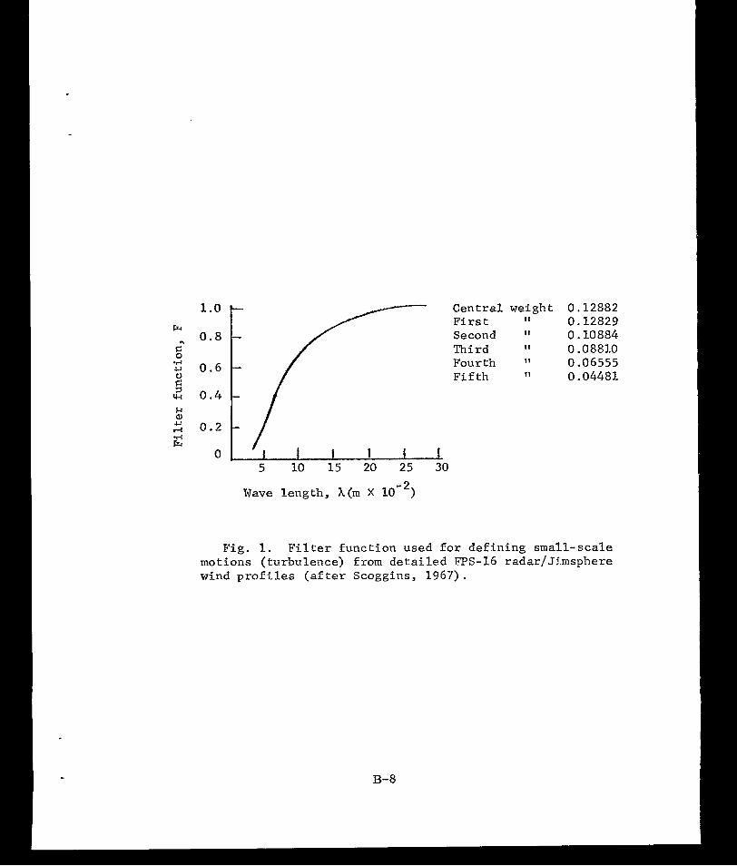
Central weight 0.12882 F i r s t 11 0.12829 Second 0.10884 Third 11 0.08810 Fourth ' I 0.06555 F i f t h I t 0.04481

F: 0 -rl u 0.6

t 8 0.4

5 10 15 20 25 30

Wave length, A (m X lom2>

Fig. 1. F i l t e r func t ion u sed fo r de f in ing small-scale motions (turbulence) from detailed FPS-16 radar/Jj.msphere wind prof i les (af ter Scoggins , 1967) .

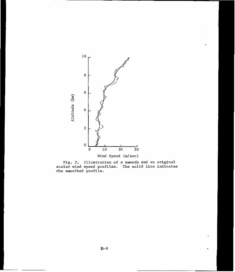
a a, 3 w

LO

0 LO 20 30

Wind Speed (m/sec)

Fig. 2. I l l u s t r a t i o n o f a smooth and an o r i g i n a l scalar wind speed profiles. The s o l i d l i n e i n d i c a t e s the smoothed p r o f i l e .

B-9

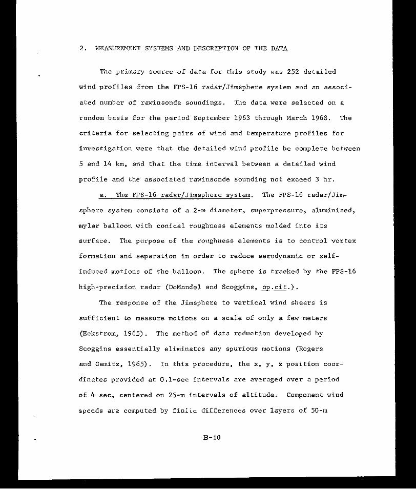
2. MEASUMMENT SYSTEMS AND DESCRIPTION OF THE DATA

The pr imary source of data for this study w a s 252 de ta i l ed

wind p r o f i l e s from the FPS-16 radar/Jimsphere system and an associ-

a t e d number of rawinsonde soundings. The da ta were se lec ted on a

random bas is for the per iod September 1963 through March 1968. The

cr i ter ia fo r s e l ec t ing pa i r s o f wind and temperature prof i les €or

i nves t iga t ion were that the de t a i l ed wind profile be complete between

5 and 14 km, and tha t t he t i m e i n t e r v a l between a de t a i l ed wind

p r o f i l e and the, associated rawinsonde sounding not exceed 3 h r .

a. The FPS-16 radar/Jimsphere system. The FPS-16 radar/Jim-

sphere system consists of a 2-m diameter, superpressure, aluminized,

mylar balloon with conical roughness elements molded i n t o i t s

sur face . The purpose of the roughness elements i s to con t ro l vo r t ex

formation and separat ion in order to reduce aerodynamic o r s e l f -

induced motions of the ba l loon . The sphere i s tracked by the FPS-16

high-precis ion radar (DeMandel and Scoggins, 9,s.). The response of the Jimsphere to ver t ical wind shears i s

s u f f i c i e n t to measure motions on a scale of only a few meters

(Eckstrom, 1965). The method of data reduction developed by

Scoggins e s sen t i a l ly e l imina te s any spurious motions (Rogers

and Camitz, 1965). I n this procedure, the x, y, z posi t ion coor-

dinates provided a t 0 .1-sec intervals are averaged over a per iod

of 4 sec, centered on 25-m i n t e r v a l s of a l t i t u d e . Component wind

speeds are computed by f i n l i s d i f f e r e n c e s ovt?~ l q e r s of 50-rn

B-IO

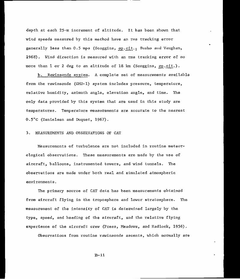
depth a t each 25-m increment of al t i tude. It has been shown t h a t

wind speeds measured by t h i s method have an rms t r ack ing e r ro r

genera l ly less than 0.5 m p s (Scoggins, op. c i t . ; Susko and Vaughan,

1968). Wind d i r e c t i o n i s measured with an rms t racking e r ror o f no

more than 1 o r 2 deg t o an a l t i t u d e of 18 km (Scoggins, 9. cit .) . b. Rawinsonde system. A complete set of measurements ava i l ab le

from the rawinsonde (GMD-1) system includes pressure, temperature,

relative humidity, azimuth angle, elevation angle, and t i m e . The

only data provided by t h i s system that are used i n t h i s s t u d y are

temperatures. Temperature measurements are accurate to t he nea res t

0.5OC (Danielsen and Duquer, 1967).

3 . MEASUFSXENTS AND OBSERVATIONS OF CAT

Measurements of turbulence are not included in routine meteor-

o logica l observa t ions . These measurements are made by the use of

aircraft, balloons, instrumented towers, and wind tunnels. The

observations are made under both real and simulated atmospheric

environments.

The primary source of CAT data has been measurements obtained

from a i r c ra f t f l y ing i n t he t roposphe re and lower stratosphere. The

measurement of the intensity of CAT is determined largely by the

type, speed, and heading of t h e a i r c r a f t , and the relative f l y i n g

experience of t h e a i r c r a f t c r e w (Press, Meadows, and Hadlock, 1956).

Observations from routine rawinsonde ascents, which normally are

B-ii

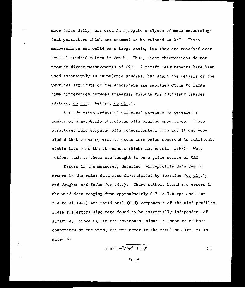
made twice d a i l y , are used in synopt ic ana lyses of mean meteorolog-

i c a l p a r m e t e r s which are assumed t o b e r e l a t e d t o CAT. These

measurements are val id on a large scale, but they are smoothed Over

several hundred meters i n depth. Thus, these observations do n o t

provide direct measurements of CAT. A i r c r a f t measurements have been

used ex tens ive ly i n t u rbu lence s tud ie s , bu t aga in t he de t a i l s of the

ver t ical s t r u c t u r e of the atmosphere are smoothed owing t o l a r g e

time differences between t raverses through the turbulent regimes

(Axford, 3. c i t . ; Reiter, 2.s.).

A s tudy us ing radars of d i f fe ren t wavelengths revea led a

number of a tmospheric s t ructures with braided appearance. These

s t r u c t u r e s were compared with meteorological data and i t was con-

c luded t ha t b reak ing g rav i ty waves were be ing obse rved i n r e l a t ive ly

s t a b l e l a y e r s o f the atmosphere (Hicks and Angell, 1967). Wave

motions such as these are thought to be a prime source of CAT.

E r ro r s i n the measured, detai led, wind-profi le data due to

e r r o r s i n t h e r a d a r d a t a were inves t iga t ed by Scoggins (op.cit .) ;

and Vaughan and Susko @. - c i t . ) . These authors found rn~s e r r o r s i n

t h e wind data ranging from approximately 0.3 t o 0 .6 mps each fo r

the zonal (W-E) and meridional (S-N) components of the wind p r o f i l e s .

These nns e r r o r s a l s o were found t o be essent ia l ly independent of

a l t i t u d e . S i n c e CAT i n t h e h o r i z o n t a l p l a n e i s composed of both

components of the wind, the rms e r r o r i n t h e r e s u l t a n t (rms-r) i s

given by

B- I 2

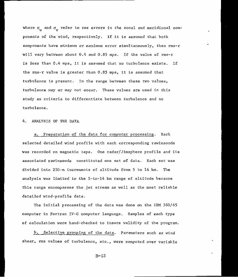
where au and av refer to rms e r r o r s i n t h e zonal and meridional com-

ponents of the wind, respectively. If i t i s assumed that both

components have minimum o r maximum error simultaneously, then rms-r

w i l l vary between about 0.4 and 0.85 mps. I f the value of rms-r

i s less than 0.4 mps, i t i s assumed tha t no tu rbu lence ex i s t s . I f

t he rrns-r value i s g rea t e r t han 0.85 mps , i t i s assumed t h a t

turbulence i s present . I n the range between these two values ,

turbulence may o r may not occur. These values are used i n t h i s

study as criteria t o d i f f e r e n t i a t e between turbulence and no

turbulence.

4. ANALYSIS OF THE DATA

a. Prepa ra t ion o f t he da t a fo r computer processing. Each

s e l e c t e d d e t a i l e d wind profile with each corresponding rawinsonde

w a s recorded on magnetic tape. One radar/J imsphere prof i le and i t s

associated rawinsonde constituted one set of da t a . Each set w a s

d iv ided i n to 250-m increments of a l t i tude from 5 t o 1 4 km. The

ana lys i s was l imi t ed to the 5-to-14 km range of a l t i tude because

th i s r ange encompasses the je t stream as w e l l as the mos t re l iab le

de ta i led wind-prof i le da ta .

The i n i t i a l p r o c e s s i n g of the da t a was done on the I B M 360 /65

computer i n F o r t r a n IV-G computer language. Samples of each type

of c a l c u l a t i o n w e r e hand-checked to i n s u r e v a l i d i t y of the program.

b. Select ive grouping of the data. Parameters such as wind

shear , n ~ ~ s values of turbulence, etc., were computed ove r va r i ab le

B- 13

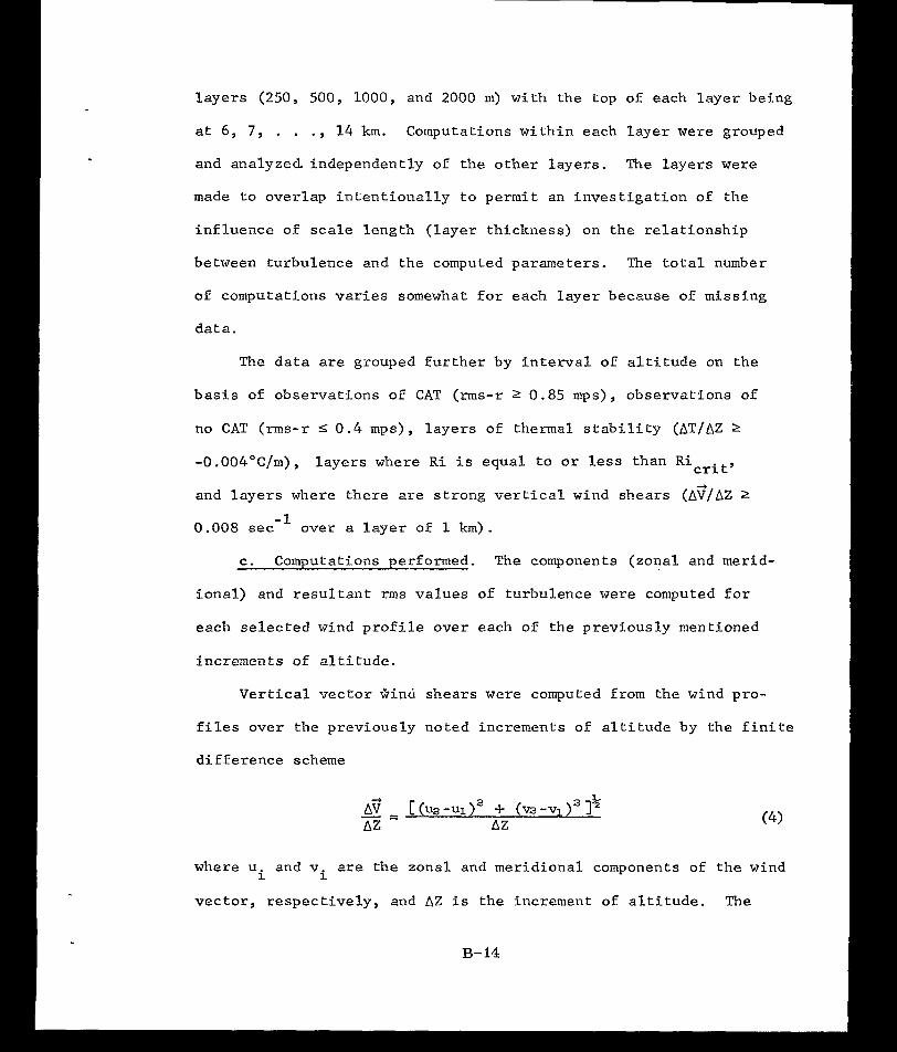
l a y e r s (250, 500, 1000, and 2000 m) with the top of each layer being

a t 6 , 7 , . . ., 1 4 km. Computations within each layer were grouped

and analyzed. independently of the other layers. The layers were

made t o o v e r l a p i n t e n t i o n a l l y t o p e r m i t an inves t iga t ion o f t he

in f luence oE scale length ( layer th ickness) on t h e r e l a t i o n s h i p

between turbulence and the computed parameters. The t o t a l number

of computations varies somewhat for each layer because o f missing

da ta .

The d a t a are grouped fur ther by in te rva l oE a l t i t u d e on the

b a s i s of observa t ions of CAT (ms-r 2 0.85 mps) , observa t ions oE

no CAT (rms-r f 0.4 mps) , l a y e r s o f t h e r m a l s t a b i l i t y ( b T / A Z 2

-0.004"C/m), layers where R i i s e q u a l t o o r less than Ricrit ,

and layers where there are s t rong ve r t i ca l wind shears (A?/AZ 2

0.008 sec over a l a y e r oE 1 km) . -I

c. Computations performed. The components (zonal and merid-

i o n a l ) and r e s u l t a n t rms va lues of turbulence were computed f o r

each s e l ec t ed wind p ro f i l e ove r each of the previously mentioned

increments of a l t i t u d e .

Vertical v e c t o r Ginit shears were computed from the wind pro-

f i l es over the p rev ious ly no ted increments o f a l t i tude by t h e E i n i t e

difEerence scheme

where u and v are the zonal and meridional components of t he wind

v e c t o r , r e s p e c t i v e l y , and A 2 i s the increment of a l t i tude. The

i i

B- 14

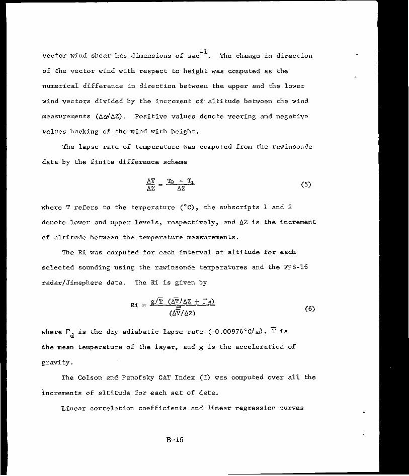
vec to r wind shear has dimensions of sec . The change i n d i r e c t i o n

of t he vec to r wind wi th respect to he igh t w a s computed as the

numer i ca l d i f f e rence i n d i r ec t ion between the upper and the lower

wind vectors divided by the increment of . a l t i tude between the wind

measurements ( A d A Z ) . Posi t ive va lues denote veer ing and negat ive

values backing of the wind wi th he ight .

-1

The lapse rate of temperature w a s computed Erom the rawinsonde

da ta by t h e f i n i t e d i f f e r e n c e scheme

where T r e f e r s to the temperature ("C), t he subsc r ip t s 1 and 2

denote lower and upper levels , respect ively, and AZ is the increment

of a l t i t u d e between the temperature measurements.

The Ri w a s computed f o r each i n t e r v a l o f a l t i t u d e f o r e a c h

selected sounding using rhe rawinsonde temperatures and the FPS-16

radar/Jimsphere

where rd i s the

data . The R i i s given by

d r y ad iaba t i c l apse rate (-O.O0976'"C/m), T i s -

t he mean temperature of the layer , and g i s the acce le ra t ion of

g r a v i t y . The Colson and Panofsky CAT' Index (I) was computed over a l l the

increments of a l t i t u d e f o r e a c h set of data .

L inea r co r re l a t ion coe f f i c i en t s and l i nea r r eg res s ion cu rves

B- 15

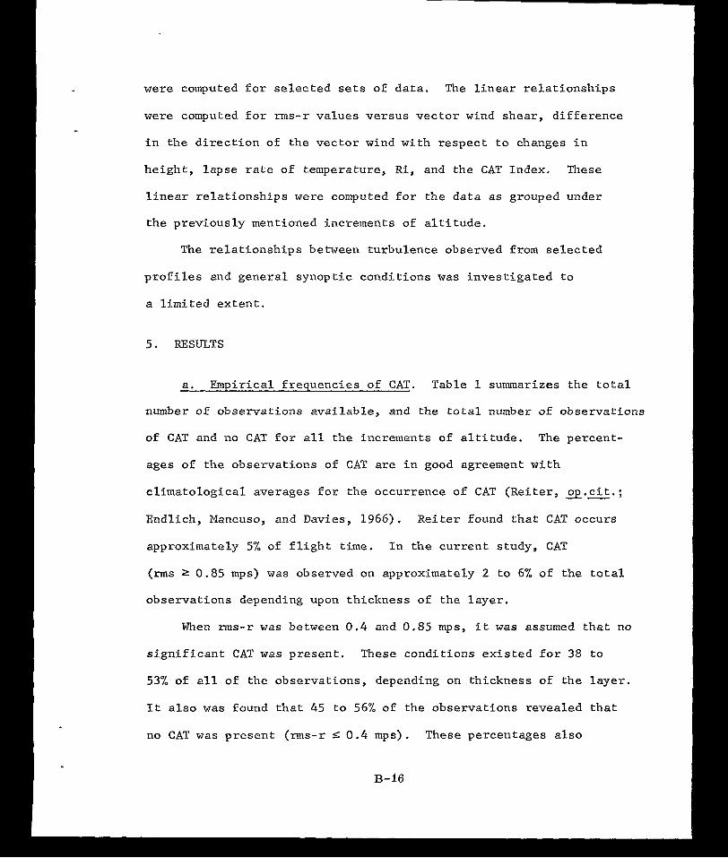
were computed f o r s e l e c t e d sets of da ta . The l i n e a r r e l a t i o n s h i p s

were computed f o r rms-r va lues ve r sus vec to r wind shea r , d i f f e rence

i n t h e d i r e c t i o n o f t h e v e c t o r wind wi th r e spec t t o changes i n

he igh t , l apse rate of temperature, R i , and the CAT Index. These

l i n e a r r e l a t i o n s h i p s were computed f o r t h e d a t a as grouped under

the p rev ious ly ment ioned increments o f a l t i tude .

The relat ionships between turbulence observed f rom selected

p r o f i l e s and genera l synopt ic condi t ions was i n v e s t i g a t e d t o

a l i m i t e d e x t e n t ,

5. RESULTS

a. Empir ical f requencies of CAT. Table I summarizes t h e t o t a l

number o f observa t ions ava i lab le , and t h e t o t a l number of observat ions

of CAT and no CAT f o r a l l t he i nc remen t s o f a l t i t ude . The percent-

ages of the observat ions of CAT are i n good agreement w i t h

c l ima to log ica l ave rages fo r t he occu r rence o f CAT (Reiter, o ~ . c i t . ;

Endlich, Mancuso, and Davies, 1966). Reiter found that CAT occurs

approximately 5% of f l i g h t t i m e . I n the cu r ren t s tudy , CAT

(rms 2 0.85 mps) was observed on approximately 2 t o 6% of t h e t o t a l

observations depending upon th ickness o f the l ayer .

When ms-r w a s be tween 0.4 and 0.85 mps, i t w a s assumed t h a t no

s i g n i f i c a n t CAT w a s p re sen t . These cond i t ions ex i s t ed fo r 38 t o

53% of a l l of the observat ions, depending on th ickness of t he l aye r .

It a l s o w a s found t h a t 45 t o 56% of the observa t ions revea led tha t

no CAT w a s p r e s e n t (rms-r 5 0.4 mps) . These percentages a l s o

B- 16

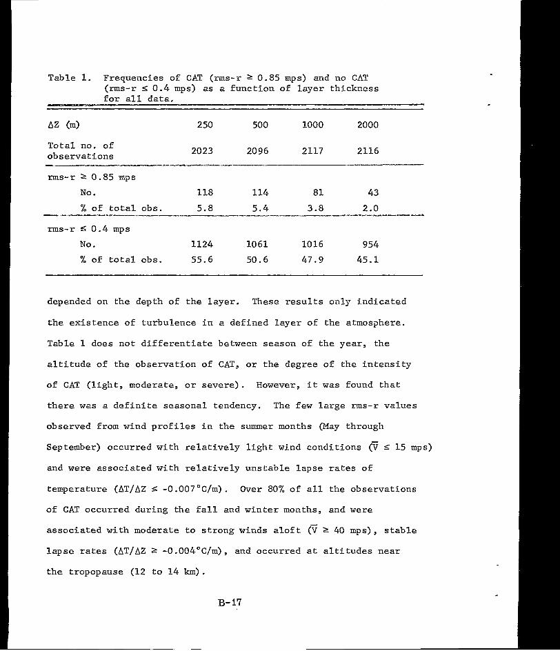
Table 1. Frequencies of CAT (rms-r 2 0.85 mps) and no CAT (rms-r I; 0.4 mps) as a func t ion of l ayer th ickness for a l l data .

7- - Az (m) 250 500 1000 2000

Tota l no. of observat ions 2023 20 96 2117 2116

rms-r 2 0.85 mps

No. 118 114 81 43 X of t o t a l obs . 5.8 5.4 3.8 2.0

ms-r 5 0.4 mps

No. 1124 1061 10 16 954 % of to t a l obs . 55.6 50.6 47.9 45.1

depended on the depth of the layer . These re su l t s on ly i nd ica t ed

the ex is tence o f tu rbulence in a def ined layer of the atmosphere.

Table 1 does no t d i f f e ren t i a t e between season of the year , the

al t i tude of the observat ion of CAT, o r the degree o f the in tens i ty

of CAT ( l igh t , modera te , o r severe) . However, i t w a s found t h a t

t he re w a s a def ini te seasonal tendency. The few l a r g e rms-r values

observed from wind p r o f i l e s i n t h e summer months (May through

September) occurred with re la t ively l ight wind condi t ions (v < 15 mps)

and were as soc ia t ed w i th r e l a t ive ly uns t ab le l apse rates of

temperature (AT/AZ i -O.O07"C/m) . Over 80% of a l l the observat ions

of CAT occurred dur ing the fa l l and win te r months, and were

associated with moderate to s t rong winds a lof t (v 2 40 mps) , s t a b l e

lapse rates (AT/AZ 2 -O.O04"C/m), and occurred a t a l t i t u d e s n e a r

the tropopause (12 t o 14 km).

B- 17

Table 2 summarizes the f requencies of observa t ions of CAT a s

a func t ion of a l t i t u d e o f o b s e r v a t i o n and thickness of t he l aye r .

In excess o f 80% of a l l the observa t ions of CAT, over a l l o f the

def ined layers , occur red a t a l t i t u d e s above 10 km. Generally, the

number of observat ions of CAT i n c r e a s e d w i t h a n i n c r e a s e i n a l t i t u d e

and decreased with an i n c r e a s e i n l a y e r t h i c k n e s s . P r e v i o u s s t a t i s -

t i c s (Endlich, Mancuso, and Davies, op. c i t .) regarding the f requency

of occurrence of CAT w i t h r e s p e c t t o a l t i t u d e a r e i.n good agreement

w i t h t h e r e s u l t s o b t a i n e d i n t h i s i n v e s t i g a t i o n . E n d l i c h , Mancuso,

and Davies found that the frequency of occurrence o f CAT increased

w i t h a n i n c r e a s e i n a l t i t u d e , and that the peak f requency w a s as h igh

as 18% of f l i g h t t i m e f o r a l t i t u d e s n e a r t h e j e t stream. In Tab le

2, t h e r e s u l t s from the p re sen t s tudy are i n q u a l i t a t i v e agreement

with those of Endlich, Mancuso, and Davies. In t he p re sen t s tudy

t h e mean height of the maximum wind speed velocity w a s observed to

be near 13 km f o r most of the cases where CAT w a s observed.

b. Relationships between CAT and se lec ted meteoro logica l

parameters. The rms-r ve r sus t he ve rb ica l wind shear , for the

e n t i r e d a t a sample , p rovided one o f the be t te r l lnear re la t ionships

found in t h i s i nves t iga t ion . L inea r r eg res s ion cu rves be tween rms-r

and v e r t i c a l wind shear are shown i n F i g . 3 . The s lopes of t he

cu rves i nc rease as the depth of the l ayer decreases . S ince an

nns-r va lue equa l t o o r g rea t e r t han 0.85 mps def ines an observa t ion

of CAT, and an rms-r va lue less than or equal t o 0.4 mps deEines

an observat ion of no CAT, t h e i n t e r s e c t i o n s of these rms-r l i n e s

B- 18

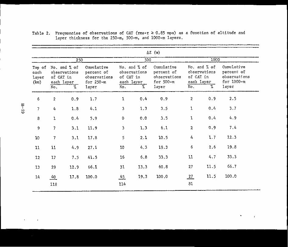
Table 2 , Frequencies of observations of CAT (rms-r 2 0.85 mps) as a f u n c t i o n o f a l t i t u d e and l aye r t h i ckness fo r t he 250-111, 500-m, and 1000-m l a y e r s ,

42 (m)

2 50 500 1000

Top of No, and % of Cumulative No, and % of Cumulative No. and % of Cumulative each observat ions pe rcen t of observat ions percent of observat ions percent of laver o f CAT i n observat ions of CAT i n observat ions of CAT i n observati.ons (&) each l aye r fo r 250-m each l aye r fo r 500-m each layer f o r 1000-m

No. X l a y e r No, % l a y e r No. l a y e r

6 2 0 . 9 1 . 7 1 0 , 4 0 . 9 2 0 . 9 2 . 5

Y CL 7 4 1 . 8 4.1 3 1 . 3 3 . 5 1 0.4 3.7 W

8 1 0 , 4 5.9 0 0 .o 3.5 1 0 . 4 4 . 9

9 7 3 . 1 1 1 . 9 3 1 , 3 6 . 1 2 0 . 9 7 . 4

10 7 3 . 1 17.8 5 2 .1 10 L 5 4 1 . 7 12.3

11 11 4.9 27.1 10 4 . 3 19.3 6 2 . 6 1 9 , 8

1 2 17 7 , 5 41.5 16 6 , 8 33 ,3 11 4.7 33 ,3

13 29 1 2 , 9 66.1 31 1 3 , 3 60.8 27 11.5 66.7

14 - 40 17.8 100.0 7 45 1 9 , 3 100,O - 27 11.5 100.0

118 114 81

. I

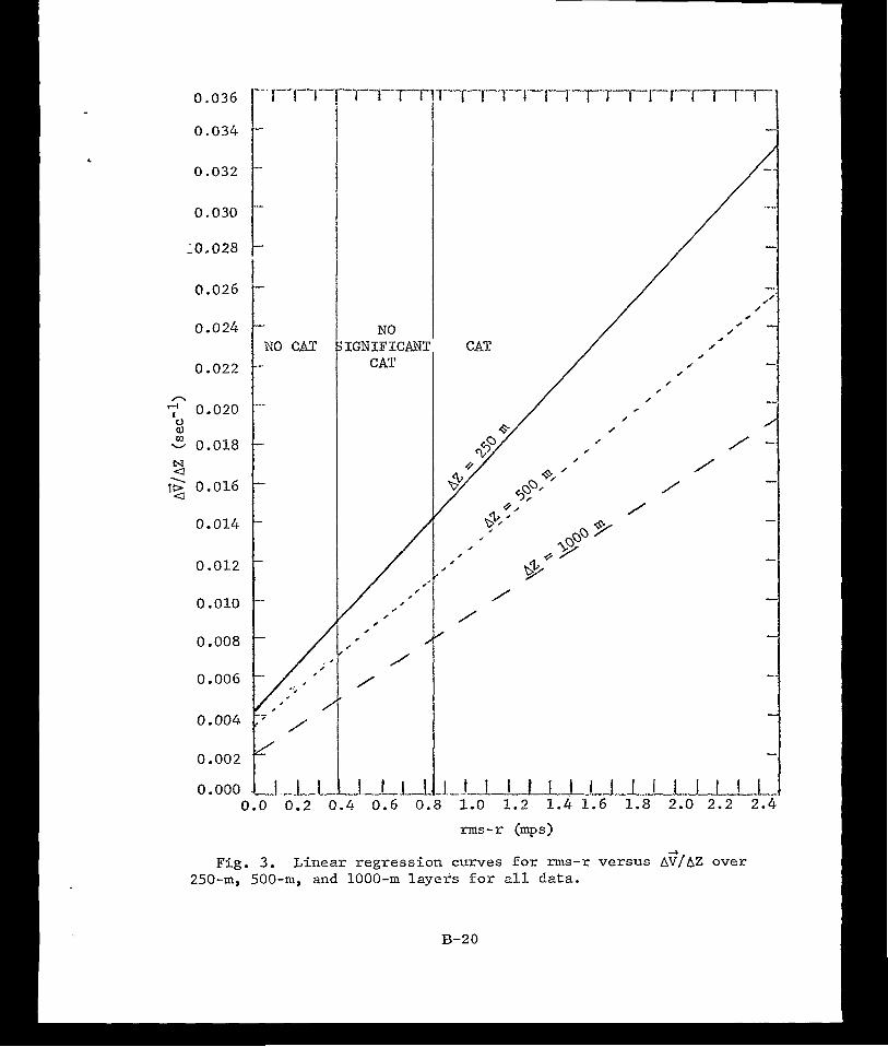
rms-r (mps)

Fig. 3. Linear regress ion curves f o r rms-r versus A?/AZ over 250-111, 500-m, and 1000-m l aye r s €o r a l l data .

B-20

w i t h t h e linear r eg res s ion cu rves de f ine "criticalft wind shears f o r

CAT and no CAT f o r the 250-111, 500-111, and 1000-m l a y e r s . The magni-

tude of t h e s e "critical" wind shears decreases as the depth of t h e

l a y e r i n c r e a s e s .

Table 3 i l l u s t r a t e s t h e f r e q u e n c i e s o f o b s e r v a t i o n s o f CAT

ve r sus t he "c r i t i ca l" wind skiears f o r CAT and no CAT. I n t h e 250-111

l a y e r , t h e "critical" wind s h e a r f o r CAT w a s equa l l ed o r exceeded

i n 415 ou t of 2023 observa t ions (22%) , b u t CAT w a s observed only 93

times (4.5%), and no CAT w a s observed 7 1 t i m e s (3.5%). In o t h e r

words , for observa t ions when the "critical" wind s h e a r w a s equa l l ed

o r exceeded, CAT o c c u r r e d i n 22% and no CAT w a s o b s e r v e d i n 17% of

these observa t ions . I n the 500-m l a y e r CAT occured i n 26% and no

CAT o c c u r r e d i n 15% of the obse rva t ions when t h e wind shea r w a s

equal to o r g r e a t e r t h a n t h e " c r i t i c a l " value. I n t h e 1000-m

l a y e r CAT occurred near ly twice as many t i m e s as no CAT f o r o b s e r -

va t ions where the wind shear equa l led o r exceeded the "critical"

value. From a comparison of Tables 1 and 3, it can be s een that over

79% of the observa t ions o f CAT f o r t h e 250-111 and 500-111 layers occur red

when t h e 'rcritical" wind s h e a r f o r each l a y e r was equa l l ed o r

exceeded, while only 31% of the observa t ions of CAT f o r t h e 1000-m

l aye r occu r red when t h e " c r i t i c a l " wind s h e a r f o r CAT i n t h i s l a y e r

was equal led o r exceeded .

For observat ions when t h e "cri t ical" wind shear €or no CAT

was not exceeded, Table 3 shows t ha t , gene ra l ly , t he obse rva t ions

of CAT increased wi th an i n c r e a s e i n l a y e r t h i c k n e s s , b u t CAT w a s

B-2 1

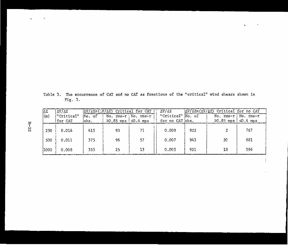
Table 3 . me Occurrence of CAT and no CAT as functions of t he " c r i t i ca l " wind shears shown i n Fig. 3 .

'" 1 AT ~AV/AZ+V/AZ) Cr i t i ca l fo r CAT I i AV/AZ iAV/AZs(AV/AZ) C r i t i c a l f o r no CAT (m) ' f c r i t i ca l " 'NO. of I NO, ms-r ; NO. ms-r i I "Cri t ical" ]NO. of i NO. ms-r 1 NO. ms-r

w jobs. I 20.85 mps 1 M .4 mps : I f o r no CAT lobs. 1 20.85 mps 150.4 mps I Lo ; I ! N 250 1 0.014 415 93 j 7 1 0.009 922 2 767 j

590 0.011 375 96 I 57 0.007 943 2c 681

1000 0.008 333 13 0 .005 921 18 596 25 1

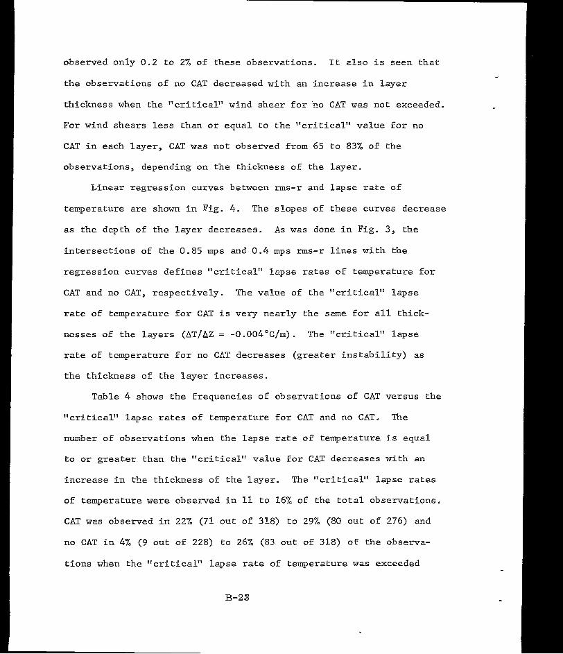
observed only 0 .2 t o 2% of these observations. It a l so is seen that

the observations of no CAT decreased with an increase i n l a y e r

thickness when the "critical" wind shear for 'no CAT w a s not exceeded.

For wind shears less than or equal to t h e " c r i t i c a l " v a l u e f o r no

CAT i n each layer, CAT w a s not observed from 65 t o 83% of the

observations, depending on the thickness of the layer.

Linear regression curves between rms-r and lapse rate of

teapera ture are shown i n Fig. 4. The slopes of these curves decrease

as the depth of the layer decreases. A s w a s done i n Fig. 3, the

in t e r sec t ions of the 0.85 mps and 0.4 mps rms-r l i nes w i th t he

regression curves def ines "cr i t ical" lapse ra tes of temperature for

CAT and no CAT, respec t ive ly . The value of the "cr i t ical" lapse

rate of temperature for CAT i s 'very near ly the same f o r all thick-

nesses of the layers (AT/BZ = -O.O04"C/m). The " c r i t i c a l " l a p s e

rate of temperature for no CAT decreases (grea te r ins tab i l i ty ) as

the thickness of the layer increases .

Table 4 shows the frequencies of observations of CAT versus the

" c r i t i c a l " lapse rates of temperature for CAT and no CAT. The

number of observations when the l apse rate of temperature i s equal

to or g rea t e r t han t he " c r i t i ca l " va lue fo r CAT decreases with an

inc rease i n t he t h i ckness of t he l aye r . The ' l c r i t i c a l l r l a p s e rates

of temperature w e r e observed i n 11 to 16% of the total observat ions.

CAT w a s observed i n 22% (71 out of 318) t o 29% (80 out of 276) and

no CAT i n 4% (9 ou t of 228) t o 26% (83. out of 318) of the observa-

t i ons when the " c r i t i ca l " l apse rate of temperature was exceeded

B-23

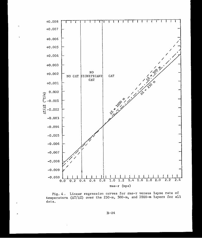
"0 .008

"0 -007 ..

"0 .006

"0 .005

+O .004

"0.003

"0 .002

"0.001

r\ 0 .ooo

", -0.001

a ' -0.002

E \ V

N

2 -0.003

-0.004

-0.005

-0 -006

-0.007

-0.008

-0.009

-0.010 C

NO IGMIFICAN'

CAT

// /'

1 1 1 , 4 0 . 6 0

/ /

1 1 1 1 1 1 l 1 1 1 1 1 1 1 1 1 1.0 1.2 1.4 1.6 1.8 2.0 2.2 2

B-24

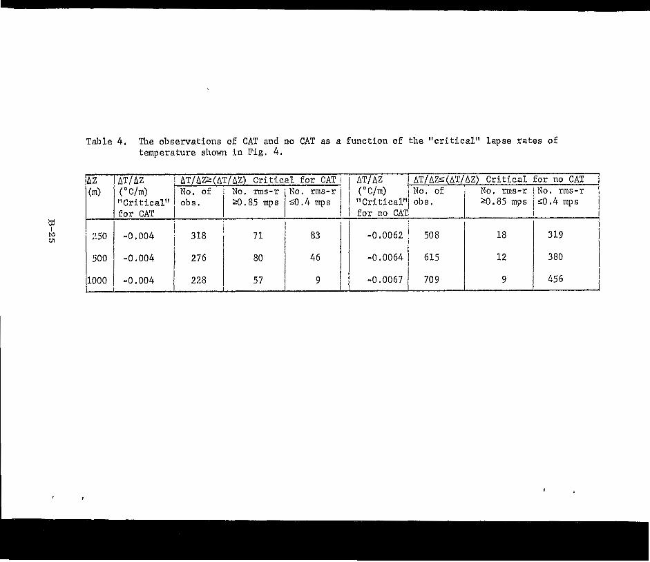
Table 4 . The observations of CAT and no CAT as a function of the "cr i t ical" lapse ra tes of temperature shown i n F i g . 4 .

Y I N 01

" ;!SO

500

1000 r

ATIU i AT/AZ>(QT/AZ) Cr i t i ca l f o r CAT i AT/AZ AT/AZg(AT/AZ) C r i t i ca l ( O CIm) NO. rms-r i N O . rms-r ("c/rn) 1 NO. of " No, ms-r

f o r CAT I 1 f o r no CAT "Cri t ical" 1 obs. Of 1 20.85 mps 1 S0.4 mps I vlCri t ical l l / obs. 20.85 mps j

i 1 -0 .004 ! 318 7 1 ' I 83 18

-0 .004 1~ 276 I 80 1 46 12

I

-0 ,004 I 228 I 57 9 709 9 1 1 -0.0067

'or no CAT No. rms-r , ~ 0 . 4 mps 1

I -,

I

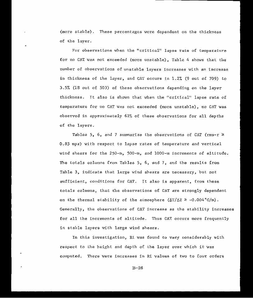
(more s t a b l e ) . These percentages were dependent on the thickness

of the l ayer .

For observat ions when the "cri t ical" l a p s e r a t e of temperature

f o r no CAT w a s not exceeded (more uns tab le) , Table 4 shows tha t t he

number of observat ions of uns t ab le l aye r s i nc reases w i th an inc rease

i n t h i c k n e s s o f the layer, and CAT o c c u r s i n 1.27, (9 ou t oE 709) t o

3.5% (18 out of 503) of these observat ions depending on t h e l a y e r

th ickness . It a l s o i s shown t h a t when t h e " c r i t i c a l " l a p s e ra te of

tempera ture for no CAT w a s not exceeded (more uns t ab le ) , no CAT was

observed i n approximately 62% of these obse rva t ions fo r a l l depths

of t h e l a y e r s .

Tables 5, 6, and 7 summarize the observa t ions o f CAT (rms-r 2

0.85 mps) w i t h r e s p e c t t o lapse ra tes of temperature and v e r t i c a l

wind s h e a r s f o r t h e 250-m, 500-my and 1000-m increments of a l t i t u d e .

The t o t a l s columns from Tables 5 , 6, and 7 , and the results from

Table 3 , i n d i c a t e t h a t l a r g e wind shea r s are necessary , bu t no t

s u f f i c i e n t , c o n d i t i o n s f o r CAT. I t a l s o i s apparent , from these

t o t a l s columns, t h a t t h e o b s e r v a t i o n s of CAT are strongly dependent

on the thermal s tab i l i ty o f the a tmosphere (AT/AZ 2 -0.004"C/m).

General ly , the observat ions of CAT inc rease as t h e s t a b i l i t y i n c r e a s e s

f o r a l l the increments o f a l t i t u d e . Thus CAT occurs more f requent ly

i n s t a b l e layers w i t h l a r g e wind shea r s .

I n t h i s i n v e s t i g a t i o n , R i was found t o vary considerably with

r e s p e c t t o t h e h e i g h t and depth of the l ayer over which i t was

computed, There were increases i n R i values of two t o f o u r o r d e r s

B-26

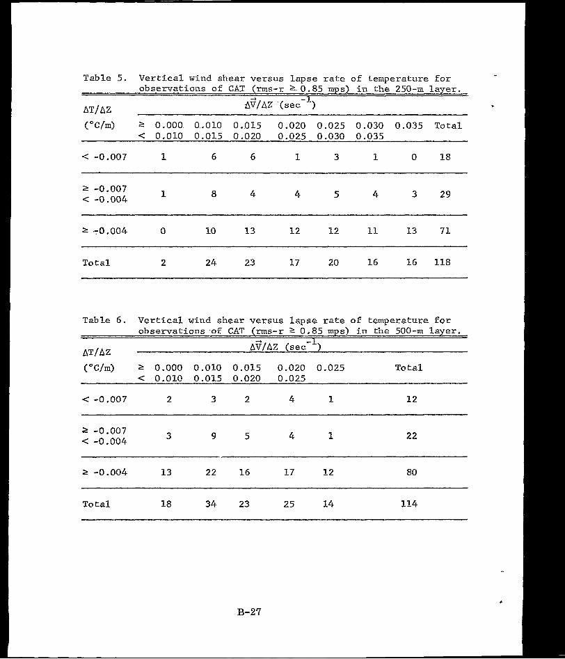
< -0.007 1 6 6 1 3 1 0 18

2 -0.007 < -0.004 1 8 4 4 5 4 3 29

2 -0.004 0 10 13 12 12 11 13 71

To ta l 2 24 23 17 20 16 16 118

Table 6 . Vertical wind shear versus l a p s e rate of temperature €or observa t ions -of CAT (rms-r 2 0.85 mps) in the 500-m l a y e r .

A T / M A?/AZ (sec-l)

("C/m) 2 0.000 0.010 0.015 0.020 0.025 To ta l < 0.010 0.015 0.020 0.025

< -0.007 2 3 2 4 1 12

2 -0.007 C -0.004 3 9 5 4 1 22

2 -0.004 13 22 16 1 7 12 80

To tal 18 34 23 25 14 114

B-27

.

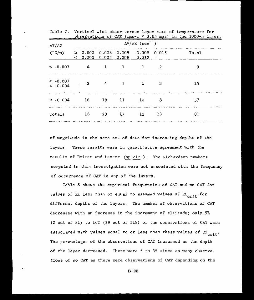
Table 7 . Vertical wind shear versus l apse ra te o f t empera ture for observat ions of CAT (rms-r 2 0.85 mps) i n t h e 1000-m l aye r .

AT/AZ Afj/A% '( sdd- ')

("C/m) 2 O..OOO 0.0.03 .0..005. 0.008 0.015. To t a l < 0.003 0.005 0.008 0.012

< -0.007 4 1 1 1 2 9

2 -0.007 < -0.004 '

2 4 5 1 3 15

2 -0.004 10 18 11 10 8 57

To ta l s 16 23 17 12 13 81

of magnitude i n t h e same set of data for increas ing depths o f the

l aye r s . These r e su l t s were i n q u a n t i t a t i v e agreement with the

r e s u l t s of Reiter and L e s t e r ( 2 . c i t . ) . - The Richardson numbers

computed i n t h i s i n v e s t i g a t i o n were not associated with the f requency

of occurrence of CAT ir? any of the l ayers .

Table 8 shows the empir ica l f requencies of CAT and no CAT f o r

va lues of Eti less than o r equa l t o assumed va lues of R i f o r

d i f f e ren t dep ths of t he l aye r s . The number of observa t ions of CAT

decreases with an inc rease i n t he i nc remen t of a l t i t u d e ; o n l y 5%

(2 out of 81) to 16% (19 out of 118) of the observat ions of CAT were

assoc ia ted wi th va lues equal to or less than these values of R i

The percentages of the observat ions of CAT increased as the depth

of the layer decreased. There were 5 t o 35 times as many observa-

t i o n s of no CAT as the re were observa t ions of CAT depending on the

c r i t

crit'

B-28

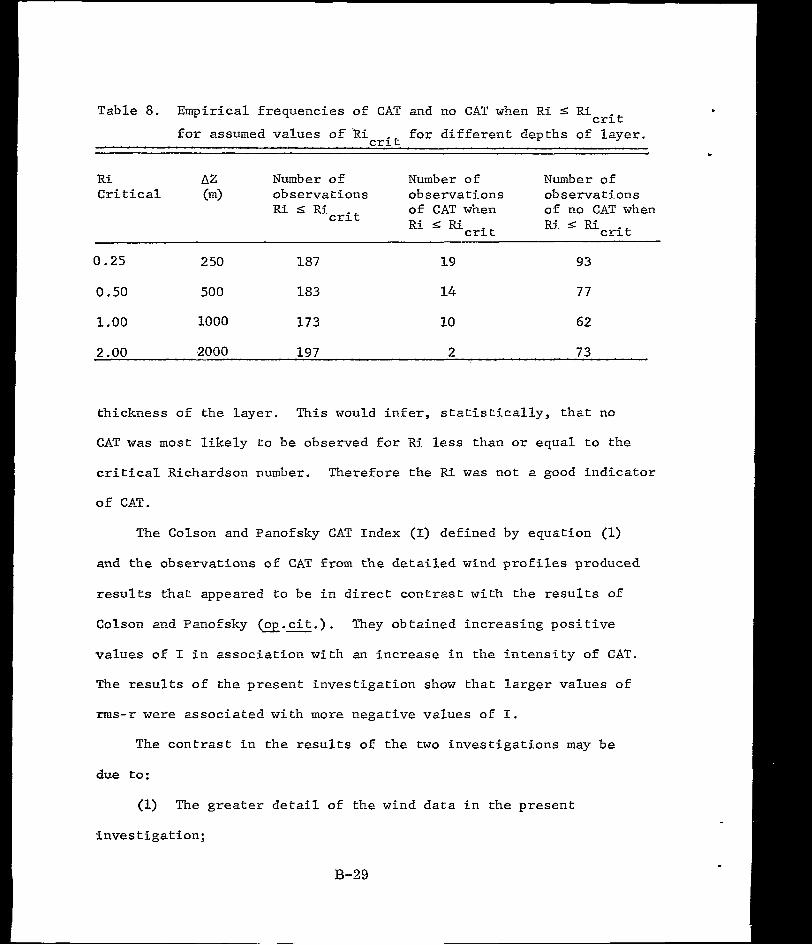
Table 8. Empir ical f requencies of CAT and no CAT when R i S R i c r i t €or assumed values o'f R i €or different depths of layer. cri t

R i A 2 Number of Number of Number of Cri t ical (m) observat ions observat ions observat ions

R i S Ricrit of CAT when of no CAT when R i Ricrit R i I R i cri t

0.25 2 50 187 19 93

0.50 500 183 14 77

1 .oo 1000 173 10 62

2 .oo ,2000 19 7 2 73

thickness of the layer , This would i n f e r , s t a t i s t i c a l l y , t h a t no

CAT w a s most l i k e l y to be observed for R i l ess than or equa l to the

critical Richardson number. Therefore the R i w a s not a good i n d i c a t o r

of CAT.

The Colson and Panofsky CAT Index (I) defined by equation (1)

and the observa t ions of CAT f r o m t h e d e t a i l e d wind prof i les produced

r e s u l t s that appeared to be i n d i r e c t c o n t r a s t w i t h t h e r e s u l t s of

Colson and Panofsky ( 2 . c i t . ) . - They ob ta ined i nc reas ing pos i t i ve

values of I i n a s s o c i a t i o n w i t h an i n c r e a s e i n t h e i n t e n s i t y of CAT.

The r e s u l t s o f t h e p r e s e n t i n v e s t i g a t i o n show t h a t l a r g e r v a l u e s o f

ms-r were assoc ia ted wi th more negative values of I.

The c o n t r a s t i n t h e r e s u l t s of the two inves t iga t ions may be

due to:

(1) The g r e a t e r d e t a i l of the wind d a t a i n t h e p r e s e n t

i nves t iga t ion ;

B-29

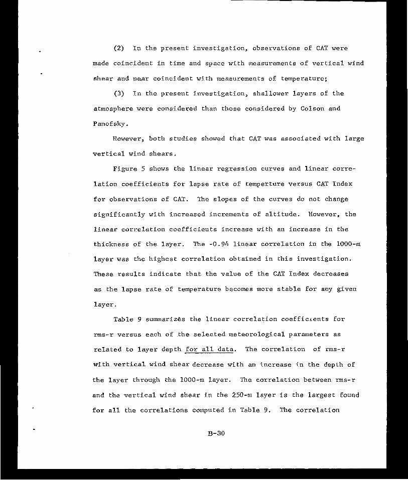
(2) In t he p re sen t i nves t iga t ion , obse rva t ions oE CAT were

made c o i n c i d e n t i n t i m e and space with measurements of vertical wind

shea r and near coincident with measurements of temperature;

(3) Zn the p resent inves t iga t ion , sha l lower l ayers o f the

atmosphere were considered than those considered by Colson and

Panof sky.

However, bo th s tud ie s showed that: CAT w a s assoc ia ted wi th l a rge

ver t ical wind shea r s .

F igure 5 shows the l i nea r r eg res s ion cu rves and l i n e a r c o r r e -

l a t i o n c o e f f i c i e n t s f o r l a p s e ra te of temperture versus CAT Index

fo r obse rva t ions o f CAT. The s lopes of the curves do not change

s ign i f i can t ly w i th i nc reased i nc remen t s o f a l t i t ude . However, the

l i n e a r c o r r e l a t i o n c o e f f i c i e n t s i n c r e a s e w i t h an i n c r e a s e i n t h e

th ickness o f the l ayer , The -0.94 l i n e a r c o r r e l a t i o n i n t h e 1000-m

l a y e r w a s t h e h i g h e s t c o r r e l a t i o n o b t a i n e d i n t h i s i n v e s t i g a t i o n .

These r e s u l t s i n d i c a t e t h a t t h e v a l u e of the CAT Index decreases

as t h e l a p s e ra te of temperature becomes more s t a b l e f o r any given

l aye r .

Table 9 summar izes t he l i nea r co r re l a t ion coe f f i cLen t s fo r

ms-r versus each of the se lec ted meteoro logica l parameters as

r e l a t e d t o l a y e r d e p t h f o r a l l da t a . The c o r r e l a t i o n of rms-r

wi th ver t ical wind shea r dec rease w i th an i nc rease i n t he dep th of

the l ayer th rough the 1000-m l a y e r . The c o r r e l a t i o n between rms-r

and the ver t ical wind shea r in the 250-m l a y e r i s the largest found

for a l l t h e c o r r e l a t i o n s computed i n T a b l e 9 . The c o r r e l a t i o n

B-30

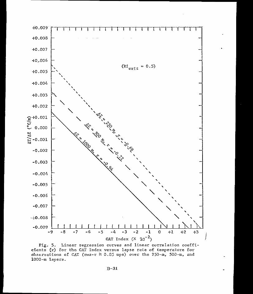
"0 .002

~#.001 \ V "- 0.000

a a

N

\ -0.001

-0.002

-0 a 003

-0 -004

-0,005

(Ricri t = 0 . 5 )

\ \ \

\ \ \

-0.306 \

\ ' \

-0.007 8

-GO -008 \ '\ \

-0 -009 -9 - 8 - 7 - 6 - 5 -4 -3 -2 -1 O +I +2 +3

CAT Tndex (X i Fig. 5 . Linea r regression curves and l inear cor re1a t i .on coef f i -

cients (r) for ths CAT Index versus lapse rate of t empera tu re fo r observations of CAT (ms-r 2 0.25 mps) over the 250-m, 5GO-m, and 1000-m l a y e r s .

33-31

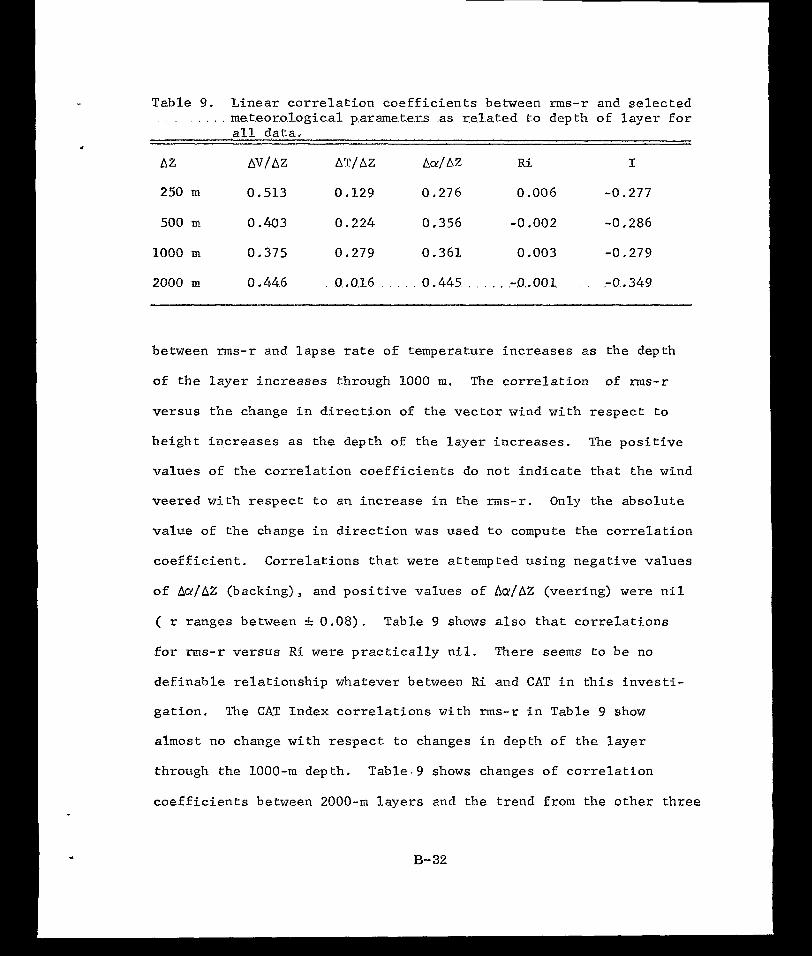
Table 9 . L i n e a r c o r r e l a t i o n c o e f f i c i e n t s between rms-r and s e l e c t e d . , . , , . rne.t.eor.o.logica1 p.arame.t.e.r.s. .as r .el .ated to depth of l a y e r f o r

.al l d a t a , . A 2 A W A Z AT/ AZ Acu/AZ Ri I

250 m 0.513 0.129 0 ,276 0.006 -0.277

500 m 0 A 0 3 0 .224 0.356 -0.002 -0.286

1000 m 0.375 0.279 0.361 0,003 -0.279

2000 m 0 .44.6 0,.0.16 . . . . 0.445 , , . . . .-(I.. O,Ol , . -0.. 349

between rms-r and lapse rate of temperature increases as the depth

of the l ayer increases th rough 1000 m. The c o r r e l a t i o n of rms-r

ver sus t he change i n d i r ec t ion of the vector wind with respect to

he igh t i nc reases as the d.epth of t h e l a y e r i n c r e a s e s . The p o s i t i v e

v a l u e s o f t h e c o r r e l a t i o n c o e f f i c i e n t s do n o t i n d i c a t e t h a t t h e wind

vee red w i th r e spec t t o an i nc rease i n t he rms- r . Only the absolu te

va lue o f t he change i n d i r ec t ion was used t o compute t h e c o r r e l a t i o n

c o e f f i c i e n t . C o r r e l a t i o n s t h a t were at tempted using negat ive values

o f Aa/AZ (backing), and p o s i t i v e v a l u e s of AcY/AZ (veering) were n i l

( r ranges between f 0 . 0 8 ) . Table 9 shows a l s o t h a t c o r r e l a t i o n s

for ms-r versus R i were p r a c t i c a l l y n i l . There seems to be no

de f inab le r e l a t ionsh ip wha teve r between R i and CAT i n t h i s i n v e s t i -

ga t ion . The CAT Index co r re l a t ions w i th nns-r i n T a b l e 9 show

almost no change with respect to changes in depth of t h e l a y e r

through the 1000-m depth. Table 9 shows changes of correlat ion

c o e f f i c i e n t s between 2000-m l a y e r s and the trend from the other three

B- 32

depths of the layers, The vertical wirid shear , d i rect ion change,

and CAT Index correlat ions increase from the values over the 1000-m

depth, whi le the correlat ion coeff ic ient for lapse rate of tempera-

t u r e shows a large decrease and the R i shows no s i g n i f i c a n t change.

These r e s u l t s imply t h a t s t a b i l i t y i n deep layers has no pronounced

e f f e c t on CAT. This could be explained by the existence of shear-

g rav i ty waves i n t h i n n e r l a y e r s t h a t would be elimlnated when

l a r g e r l a y e r s are considered.

Correlations were computed for observat ions OE CAT (rms-r 2

0.85 mps) and for observat ions of no CAT (rms-r S 0.4 mps) versus

each of the selected meteorological parameters. With the exception

of the lapse rate of temperature versus I when turbulence occurred,

t h e r e s u l t s show no s i g n i f i c a n t c o r r e l a t i o n (r ranges between

& 0.075).

Figure 6 i l l u s t r a t e s t h e c h a r a c t e r of the wind-profi le data used

i n t h i s s t u d y . CAT w a s observed i n t h i s p r o f i l e i n t h e 10 to 12 km

l ayer . The rms-r f o r t h e 250-m layer, topped a t 11 km, w a s 2.015 mps.

The l apse rate of temperature was -0.004"C/m, t h e v e r t i c a l wind

shear w a s 0.0285 sec , R i w a s 1.3, and the CAT Index w a s -80. I n

a l a r g e number of cases CAT w a s observed t o exis t over deeper

l aye r s of t he atmosphere (1000 m t o 2000 m) i f t h e r e w a s a not iceable

maximum of wind v e l o c i t y e i t h e r above o r below a s t a b l e l a y e r

(mostly below). These conditions represent strong wind s h e a r i n a

s tab l e layer .

-1

B-33

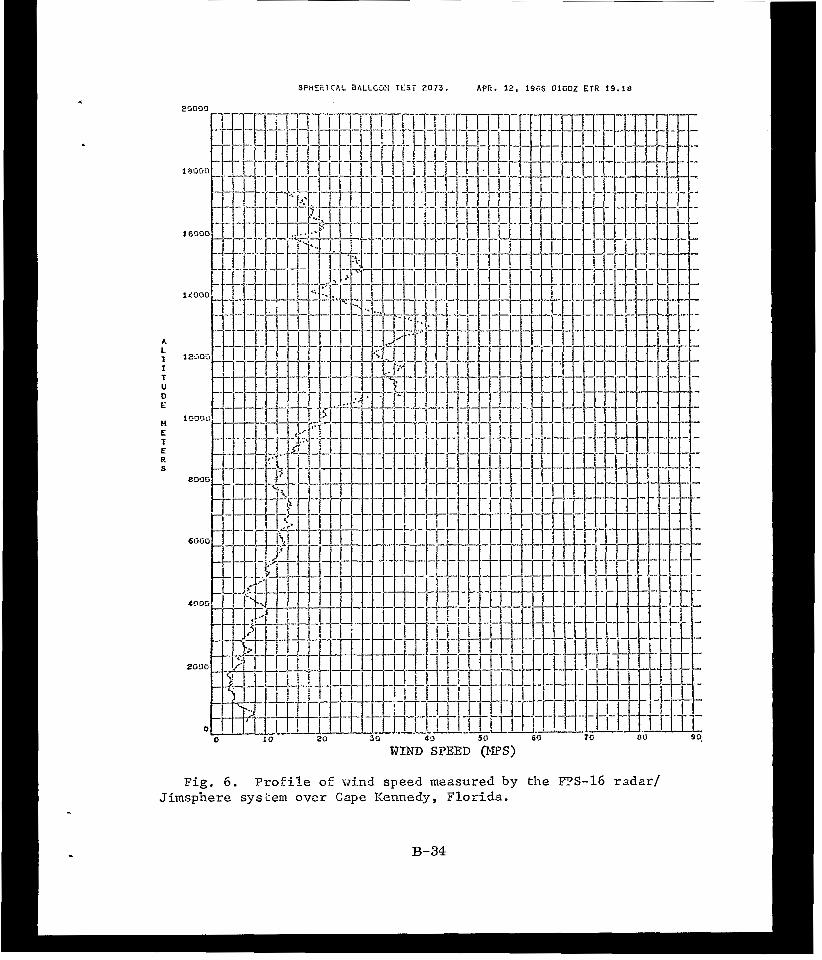
A L T I T

0 u E

H E

E T

R S

SPHEiiXCAL BALLOX TEST 2073. APE. 12. 1Sib O l G O Z ETR 19.18

Fig. 6 . P r o f i l e 05 wind speed measured by the E'S-16 radar/ Jimsphere sysirem over Cape Kennedy, Florida. -

. B-34

6. FORECASTING OF CAT

Rawinsonde measurements tend to provide underestimates of

vertical wind shear and lapse rate of temperature. The l imi t a t ions

in the meteorological data provided by t h i s system prevent detailed

analysis of CAT from these wind and temperature profiles. Without

adequate data, inaccurate analysis results. Unless there i s an

accurate analysis of data, a good fo recas t i s l i t t l e more than luck.

The r e s u l t s of t h i s i n v e s t i g a t i o n i n d i c a t e that.CAT w a s observed

i n t h i n l a y e r s of the atmosphere characterized by l a rge vertical

wind shear and s t a b l e t h e r m a l s t r a t i f i c a t i o n . .Any a t t e m p t to fore-

cast CAT must be directed toward ident i fying the regions that appear

favorable for the occurrence of CAT.

The i d e n t i f i c a t i o n o f a region where there i s CAT i s only half

of the problem involved in forecasting CAT. There is d i f f i c u l t y i n

considering a t i m e and space extrapolation of a region of CAT.

Does the region of CAT maintain i t s s i ze , shape, and in tens i ty wi th

respec t to changes i n t i m e and space? The p resen t i nves t iga t ion

cannot hypothesize on answers to this question.

The resul ts presented previously show t h a t i n o r d e r to fo recas t

CAT, the lapse rate of temperature and vertical wind s h e a r i n l a y e r s

1000 m and less in depth must be forecas t . CAT occurs predominantly

i n l aye r s w i th r e l a t ive ly s t ab le l apse rates of temperature and

with s t rong wind shear. Strong wind shear alone is not a s u f f i c i e n t

p red ic to r of C L T -

B-35

,

.

7. CONCLUSIONS AND RECOMMFNDATIONS

a . Conclusions. The inves t iga t ion of the da ta from 252 FYS-16

radar/Jimsphere detailed wind prof i les ind ica ted tha t these da ta

a re an excellent source of information on CAT.

Although vertical wind shear showed the h ighes t cor re la t ion

with the observed rms-r values, many events of CAT (rms-r 2 0.85 mps)

were observed where the "cri t ical" wind shear indicated that no CAT

should occur for the d i f fe ren t depths of the layers (see Table 3) . In this study, 'over 80% of the total observat ions of CAT

(rms-r 2 0.85 mps) were a t a l t i t u d e of 10 km and higher. Over 80%

of the total observat ions of CAT at these a l t i t udes were observed

i n r e l a t i v e l y s t a b l e l a y e r s (AT/AZ 2 -O.O04"C/m) and with large

wibd shears (AV/AZ 2 0.008 sec" over 1 km) . Based on the r e su l t s

of this s tudy, the exis tence of a la rge wind shear was not a

suf f ic ien t c r i te r ion for the occur rence of CAT.

This s tudy i l lustrates that the Richardson number i s not useful

as an ind ica to r of the existence o r i n t e n s i t y of CAT. I n t h i s same

vein, the Colson and Panofsky CAT Index showed remarkable correlation

with the lapse rate of temperature for observations of CAT

(rms-r 5: 0.85 mps). This w a s a d e f i n i t e i l l u s t r a t i o n of the poss ib le

e f f e c t of shear-gravity waves on the occurrence of CAT. This is

because the large negative values of the Index come from s t a b l e

layers wi th l a rge wind shears.

Data from the upper atmosphere must be coincident in t ime and

space with the occurrence of turbulence in order to reduce the

B- 36

s u b j e c t i v i t y of acutal observations of CAT. Any attempt to e s t a b l i s h

criteria for the occurrence of CAT must be channeled towards

i d e n t i f i c a t i o n of the mesoscale regions of the atmosphere that are

favorable for the occurrence of CAT. The current synoptic rawin-

sonde network does not provide observations of the scale and

reso lu t ion requi red to i d e n t i f y a l l regions favorable for the

occurrence of CAT.

General ly , the resul ts of this s tudy support thehypothesis

p u t f o r t h by Kuettner (1952), viz . , that unstable shear-gravity

waves occur i n and near certain regions of maximum wind bands,

and tha t these waves are a prime source of CAT.

b . Recommendations. Further s tudies of CAT using FPS-16 radar /

Jimsphere wind profiles should be made by analyzing serial p r o f i l e s

made j u s t a f e w minutes t o a f e w hours apart under conditions

suspected t o be favorable for the occurrence of CAT.

There should be an attempt t o develop an empirical method to

compute v e r t i c a l motion in the upper atmosphere from t h e d e t a i l e d

wind p r o f i l e s and associated GMD data. This i s an attempt to

measure some other meteorological parameter that might be use fu l

i n i den t i fy ing r eg ions o f CAT.

An FPS-16 radar /J imsphere s i te should be es tabl ished somewhere

i n t h e lee of the Rocky Mountains where there would be a l a r g e

volume of a i r t r a f f i c f o r a source of support ing pi lot reports of

CAT. P a s t s t u d i e s of CAT associated with mountain waves could be

re-examined using these highly accurate wind data. Most important,

B-37

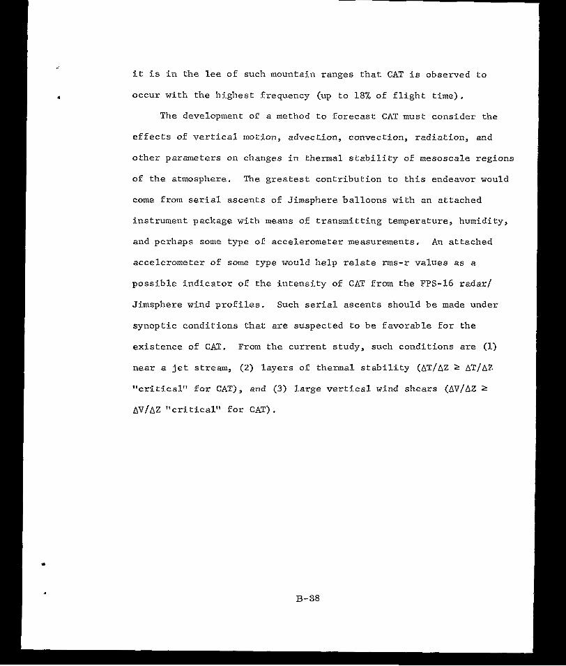
i t i s i n t h e lee of such mountain ranges that CAT is observed to

occur with the highest f requency (up t o 18% o f f l i g h t t i m e ) .

The development of a method t o f o r e c a s t CAT must consider the

e f f ec t s o f ve r t i ca l mo t ion , advec t ion , convec t ion , r ad ia t ion , and

o ther parameters on changes in thermal s tab i l i ty of mesoscale regions

of the atmosphere. The g rea t e s t con t r ibu t ion t o t h i s endeavor would

come from serial ascents of Jimsphere balloons with an attached

instrument package with means of t ransmit t ing temperature , humidi ty ,

and perhaps some type of accelerometer measurements. An a t t ached

accelerometer of some type would help relate nns-r values as a

p o s s i b l e i n d i c a t o r of t h e i n t e n s i t y of CAT from the FPS-16 r ada r /

J imsphere wind prof i les . Such serial ascents should be made under

synop t i c cond i t ions t ha t are suspected to b e f a v o r a b l e f o r t h e

ex i s t ence of CAT. From the cur ren t s tudy , such condi t ions are (1)

near a je t stream, (2) l a y e r s o f t h e r m a l s t a b i l i t y (AT/AZ 2 AT/AZ

"critical" €or CAT), and (3) l a r g e ver t ical wind shea r s (AV/AZ 2

AV/AZ "cr i t ical" €or CAT).

REFERENCES FOR APPENDIX B *

Axford, D. N . , 1968; "On t h e Accuracy of Wind Measurements Using b

a n I n e r t i a l P l a t f o r m i n a n , A i r c r a f t and an Example of a Measure- ment o f . . t h e .Vertical Mesostructure of the Atmosphere," Jou rna l of Applied Meteorology, 2, 645-666,

C l e m , L. H., 1957: "Clear A i r Turbulence from 25,000 to 45,000 Fee t over the Uni ted States,'1 AWS TR 105-47, Headquarters A i r Weather Service (MATS), Scott AFB, I l l i n o i s , 13 pp.

Colson, D. and H. A. Panofsky, 1965: "An Index of Clear A i r TUrbulence," Quart. J. R. Meteor. S O C . , 91, 507-512.

Danielsen, E. F. and R. T. Duquet, 1967: *lA Comparison of FPS-16 and GMD-1 Measurements and Methods f o r P r o c e s s i n g Wind Data," Journal of Applied Meteorology, 2, 824-836.

DeMandel, R. E. and J. R. Scoggins, 1967: "Mesoscale Wave Motions as Revealed by Improved Wind P r o f i l e Measurements," Journa l o f Applied Meteorology, 5, 617-620.

Eckstrom, Clinton V., 1965: "Theoretical Study and Engineering Development of Jimsphere Wind Sensor," Final Report , NASA Contract No. NAS8-1158, 78 pp.

Endlich, R. M. and J. W. Davies, 1967: "The F e a s i b i l i t y o f Measuring Turbulence Tn the F ree Atmosphere from Rising Balloons Tracked by FPS-16 Radar," Journal of Applied Meteorology, 5 , 43-47.

Endlich, R. M. and R. L. Mancuso, 1965: "Object ive Analysis an ' d Forecas t ing of Clear A i r Turbulence," Final Report , Contract Cwb-10871, S tan fo rd Resea rch In s t i t u t e , Menlo Park, Ca l i fo rn ia , 56 pp.

Endlich, R. M., R. L. Mancuso, and J. W. Davies, 1966: "Techniques for Determining a World Wide Climatology of Turbulence through U s e of Meteorological D a t a , " AFCRL-66-355, S c i e n t i f i c R e p o r t 1, Contract AF 19 (628)-5173, 'Stanford Research I n s t i t u t e , Menlo Park , Cal i forn ia , 62 pp.

Fo l t z , H. P., 1967: "The P r e d i c t i o n of Clear A i r Turbulence," Atmospheric Seience Paper No. 106, Department of Atmospheric Science, Colorado State Universi ty , Fort Col l ins , 145 pp.

B-39

8

Hardy, K. R. and Hans Ot t e r s t en , 1968: "Radar and A i r c r a f t I n v e s t l - g a t i o n of Clear-Air-Turbulence,' ' Proceedings of the Third National Conference on Aerospace Meteorology, American Meteorological.Society, Boston, 539-546.

Hicks, J. J. and J. K. Angell, 1967: "Radar Observations of Breaking G r a v i t a t i o n a l Waves i n t h e V i s u a l l y Clear Atmosphere," Journa l of Applied Meteorology, L , 114-121.

Kuettner, J. P., 1952: "On the Poss ib i l i ty o f Soar ing on Trave l ing Waves i n t h e Jet Stream," Aeronaut. Eng. Rev., ll, 1-7.

Lumley, J. L. and H. A. Panofsky, 1964: The S t ruc tu re of Atmospheric Turbulence, John Wiley and Sons, New York, 239 pp.

Moore, R. L. and T. N . Krishnamurti , 1966: "A Theory of Generation of CAT," Douglas Paper 3801, presented a t Nat iona l A i r Meeting on Clear A i r Turbulence, February 23, 1966, 20 pp.

Press , H., May T. Meadows, and Ivan Hadlock, 1956: "A Reevaluation of Data on Atmospheric Turbulence and Airplane Gust Loads for Appl ica t ion in Spec t ra l Calcu la t ions ," Repor t No. 1272, National Advisory Committee for Aeronaut ics , 29 pp.

Reiter, E. R . , 1963: "Nature and Observation of High Level Turbulence Espec ia l ly in Clear A i r , " Technical Paper No. 41, Department of Atmospheric Science, Colorado State University, Fo r t Co l l in s , 28 pp.

Reiter, E. R. and P. F. Lester, 1967: '!The Dependence of the Richardson Number on Scale Length," Atmospheric Science Paper No. 111, Department of Atmospheric Science, Colorado State Universi ty , Fort Col l ins , 39 pp.

Rogers, R. R. and H. A. Camitz, 1965: "Project Baldy - An I n v e s t i - g a t i o n of Aerodynamically-Induced Balloon Motions," Final Report, NASA Contract No. NAS8-1140, 80 pp.

Sawyer, J. S. 1961: "Quasi-Periodic Wind Var ia t ions wi th Height in the Lower-Stratosphere," Quart . Journ. Royal Met. SOC., 87, 24-33.

Scoggins, J. K., 1967: "Sphere Behavior and the Measurement of Wind 'Prof i les ,11 NASA TN D-3994, 53 pp.

Susko, Michael and W. W. Vaughan, 1968: "Accuracy of Wind Data Obtained by Tracing Jimsphere Wind Sensors Simultaneously with Two FPS-16 Radars,'' NASA TMX-53752, George C. Harsha l l Space Flight Center, Huntsvil le, Alabama, 48 pp.

Weinstein, A. E., E. R. Reiter and J. R. Scoggins, 1966: "Mesoscale St ruc tu re of 11-20 km Winds," Journal of Applied Meteorology, - 5, 49-57.

B-41

NASA-Langley, 1970 - 20 mFC-RSA. Ala

f. - NASA · OF TIME AT CAPE KENNEDY, FLORIDA by Jltnzes R. Scoggim, M. M. Perzdepst, arid V, E....

Documents

Transcript of f. - NASA · OF TIME AT CAPE KENNEDY, FLORIDA by Jltnzes R. Scoggim, M. M. Perzdepst, arid V, E....