Extreme Value Analysis of Wind Speed Observations over ... · Table 2.1 shows a list of the...

Arbeitsbericht MeteoSchweiz Nr. 219

Extreme Value Analysis of Wind Speed Observations over Switzerland P. Ceppi, P.M. Della-Marta, C. Appenzeller

Herausgeber Bundesamt für Meteorologie und Klimatologie, MeteoSchweiz, © 2008 MeteoSchweiz Krähbühlstrasse 58 CH-8044 Zürich T +41 44 256 91 11 www.meteoschweiz.ch

Weitere Standorte CH-8058 Zürich-Flughafen CH-6605 Locarno Monti CH-1211 Genève 2 CH-1530 Payerne

Arbeitsbericht MeteoSchweiz Nr. 219

Extreme Value Analysis of Wind Speed Observations over Switzerland P. Ceppi, P.M. Della-Marta, C. Appenzeller

Bitte zitieren Sie diesen Arbeitsbericht folgendermassen Ceppi, P., Della-Marta, P.M., Appenzeller, C.: 2008, Extreme Value Analysis of Wind Speed Observations over Switzerland, Arbeitsberichte der MeteoSchweiz, 219, 48pp.

Abstract

Accurate assessment of the magnitude and frequency of extreme wind speed is of fundamentalimportance for many safety, engineering and financial applications. However, extreme windsare coupled with local, small-scale phenomena, so that their spatial distribution is very inho-mogeneous. So far, only limited information on extreme wind statistics was available for Swissmeasuring stations.

We estimate the return period (frequency) of extreme wind speeds at 55 measuring stationsover Switzerland. We utilise daily maximum 1-second wind gust measurements for the period1981 - 2007 in order to create a local-scale extreme wind climatology. These measurements arechecked for quality to ensure that they are suitable for an extreme value analysis, and theirseasonal and long-term variability is examined.

In our analysis, we apply classical peak over threshold (POT) extreme value analysis tech-niques to the extreme wind data. Autocorrelation in the POT series is first eliminated byusing a standard declustering technique; the series are then modelled using a Generalised ParetoDistribution (GPD) which is fitted using maximum likelihood estimation (MLE). We includedestimates of the uncertainty in the return level and return period of extreme winds, which werecalculated using likelihood profile methods.

Our results show that the data quality is generally good, with no obvious jumps or outliers; nolong-term trends were visible. Generally, the choice of threshold and the declustering techniqueresult in very good model fits. At some stations, however, the peaks deviate systematically fromthe model fit. Regional differences in wind climatologies, expected due to orography, are wellreproduced. In particular, the exposure to westerly and Fohn winds seems to play a key role inthe extreme wind distribution. However, the shape of the GPD model fits is quite homogeneous;they all have an upper bound, with one exception. The return periods of selected storms alsofeature large variability from one station to another; return periods for the storm Lothar rangefrom <2 to >100 years, with most values on the Swiss Plateau lying above 10 years. Thisvariability reflects the very complex behaviour of extreme winds at surface level.

Contents

1 Introduction 61.1 Project background . . . . . . . . . . . . . . . . . . . . . . . . . . . . . . . . . . . 61.2 Practical applications . . . . . . . . . . . . . . . . . . . . . . . . . . . . . . . . . 6

2 Datasets and Data Quality 72.1 Datasets . . . . . . . . . . . . . . . . . . . . . . . . . . . . . . . . . . . . . . . . . 72.2 Data Quality . . . . . . . . . . . . . . . . . . . . . . . . . . . . . . . . . . . . . . 8

3 Extreme Value Analysis 103.1 Definition . . . . . . . . . . . . . . . . . . . . . . . . . . . . . . . . . . . . . . . . 103.2 The Peak Over Threshold (POT) method . . . . . . . . . . . . . . . . . . . . . . 103.3 Declustering and threshold selection . . . . . . . . . . . . . . . . . . . . . . . . . 123.4 Uncertainty calculations . . . . . . . . . . . . . . . . . . . . . . . . . . . . . . . . 12

4 Results 144.1 Extreme wind distribution at Swiss stations . . . . . . . . . . . . . . . . . . . . . 144.2 Spatial variation of GPD parameters . . . . . . . . . . . . . . . . . . . . . . . . . 184.3 Return levels and return periods . . . . . . . . . . . . . . . . . . . . . . . . . . . 20

4.3.1 Return periods of given wind speeds . . . . . . . . . . . . . . . . . . . . . 204.3.2 Return levels of given return periods . . . . . . . . . . . . . . . . . . . . . 20

4.4 Return period of some prominent wind storms . . . . . . . . . . . . . . . . . . . 234.5 Block Maxima method and comparison with POT analysis . . . . . . . . . . . . 26

5 Discussion and Recommendations for Further Research 295.1 Discussion of the results . . . . . . . . . . . . . . . . . . . . . . . . . . . . . . . . 295.2 Recommendations for further research . . . . . . . . . . . . . . . . . . . . . . . . 30

A Extreme wind climatologies 31

2

List of Tables

2.1 List of stations. Numbers in the first and fourth columns refer to the stationnumbers in figure 2.1. . . . . . . . . . . . . . . . . . . . . . . . . . . . . . . . . . 8

4.1 Parameters of the GPD and GEV models at station Zurich / Fluntern. . . . . . . 274.2 Comparison of the return periods obtained from a) the GPD and b) the GEV

model at station Zurich / Fluntern. . . . . . . . . . . . . . . . . . . . . . . . . . 274.3 As in table 4.2 for the four storms displayed on figures 4.10 and 4.11. . . . . . . . 28

3

List of Figures

2.1 Spatial distribution of stations used in this study. The station numbers refer tothe numbers in table 2.1. . . . . . . . . . . . . . . . . . . . . . . . . . . . . . . . 7

2.2 Daily maximum wind gusts 1981-2007 in Zurich / Kloten. The red curve is acubic smoothing spline of the measurement series, for better visualisation of thelong-term variability. This plot also gives an impression of the magnitude and fre-quency of extreme wind gusts. The highest visible peak (26.12.1999) correspondsto the storm Lothar. . . . . . . . . . . . . . . . . . . . . . . . . . . . . . . . . . . 9

3.1 Influence of a) the shape parameter ξ and b) the scale parameter σ on the GPDcurve. . . . . . . . . . . . . . . . . . . . . . . . . . . . . . . . . . . . . . . . . . . 11

3.2 a) Modified scale, σ∗ (see Coles, 2001), b) shape, ξ, and c) mean exceedance pa-rameter diagnostic plots for selecting the fixed threshold above which the declus-tered POT will be modelled using the GPD. The vertical black lines denote the95% confidence intervals calculated using the parametric resampling techniquedetailed in section 3.4. The numbers aligned vertically in the top of the plot arethe number of peaks above a given threshold. The vertical red line represents theselected threshold, corresponding to the 90% quantile. . . . . . . . . . . . . . . . 13

4.1 RL as a function of RP at Zurich / Fluntern station. The blue curve representsthe GPD fit and the black dots are the declustered peaks of the POT series. Thegreen curves show the upper and lower bounds of the 95% confidence interval.The dates of the four most extreme events are shown. Note the log scale on thehorizontal axis. . . . . . . . . . . . . . . . . . . . . . . . . . . . . . . . . . . . . . 15

4.2 As for figure 4.1 for six other stations. For more examples see Appendix A. . . . 164.3 Quantile-quantile plots for the six stations shown in figure 4.2. . . . . . . . . . . 174.4 Spatial distribution of threshold values (in m/s). . . . . . . . . . . . . . . . . . . 184.5 Spatial distribution of the shape parameter (ξ). . . . . . . . . . . . . . . . . . . 194.6 Spatial distribution of the scale parameter (σ). . . . . . . . . . . . . . . . . . . . 194.7 Spatial distribution of the lambda parameter (λ). . . . . . . . . . . . . . . . . . . 194.8 Return period of wind gusts of a) 25, b) 30 and c) 35 m/s. . . . . . . . . . . . . 214.9 RLs corresponding to RPs of a) 2, b) 5, c) 10 and d) 50 years. . . . . . . . . . . 224.10 Return periods (in years) of storms a) Lothar (26 December 1999) and b) Wilma

(26 January 1995). . . . . . . . . . . . . . . . . . . . . . . . . . . . . . . . . . . . 244.11 As for figure 4.10 for a) storm Vivian (27 February 1990) and b) an unnamed

storm (24 March 1986). . . . . . . . . . . . . . . . . . . . . . . . . . . . . . . . . 254.12 Return periods of an unnamed Fohn storm (8 November 1982). . . . . . . . . . . 264.13 Comparison between the GPD fit (left) and the GEV model fit (right) . . . . . . 27

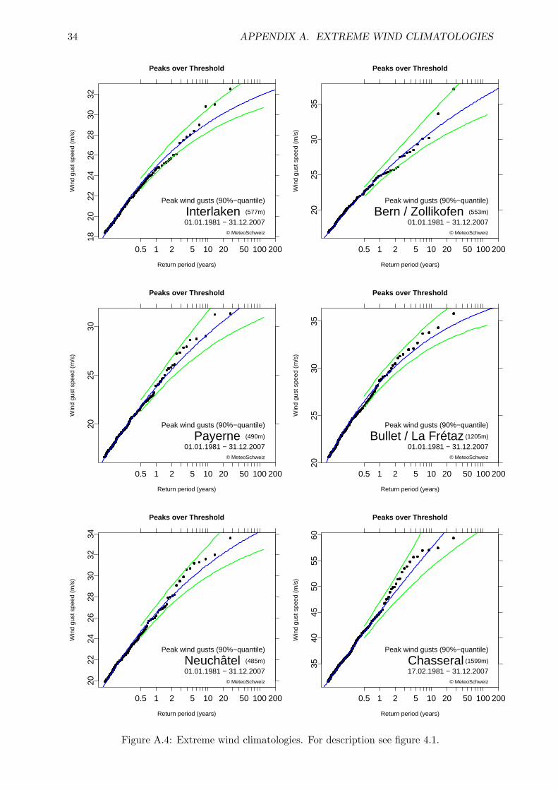
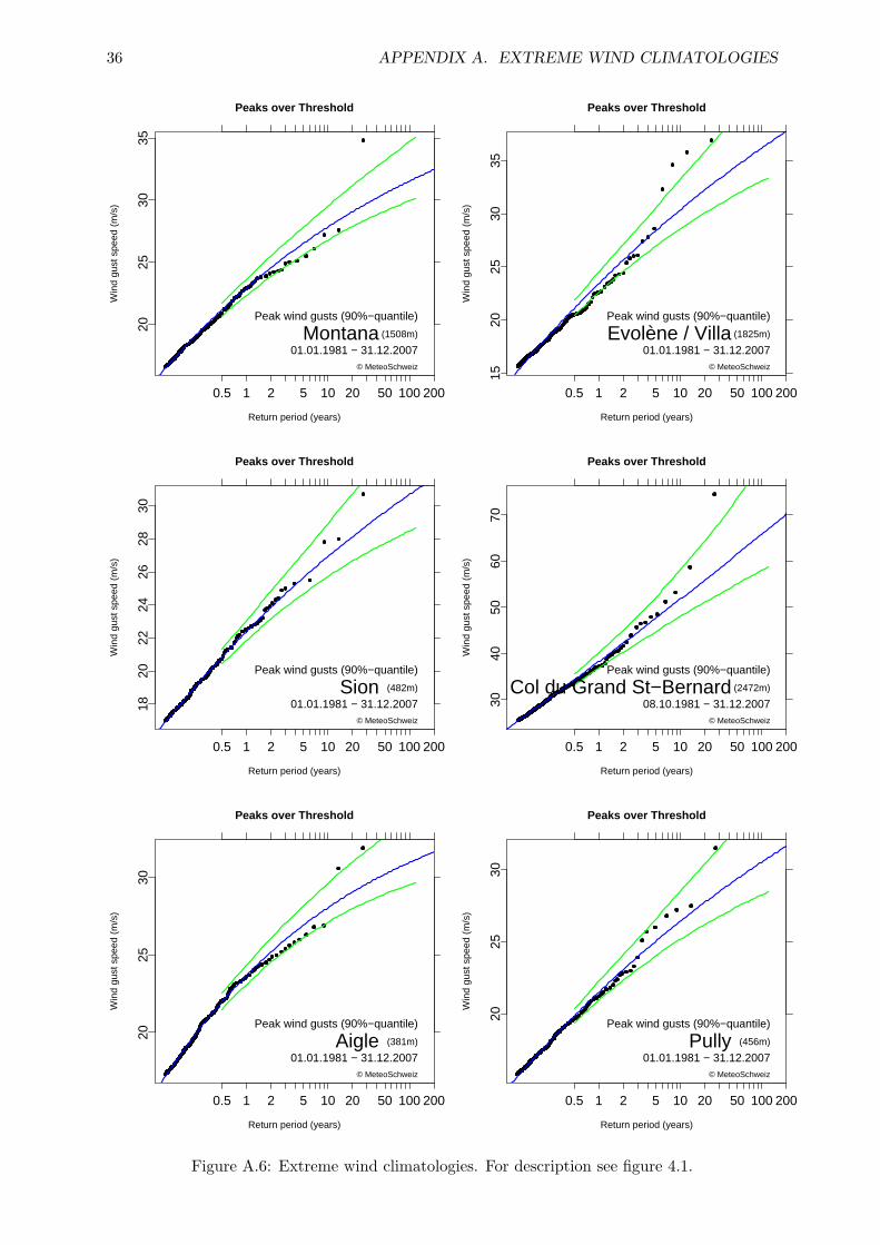
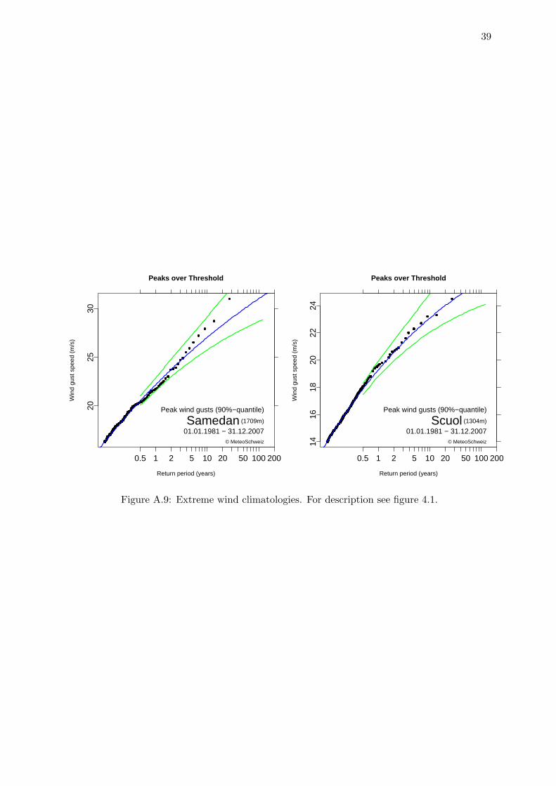
A.1 Extreme wind climatologies. For description see figure 4.1. . . . . . . . . . . . . . 31A.2 Extreme wind climatologies. For description see figure 4.1. . . . . . . . . . . . . . 32A.3 Extreme wind climatologies. For description see figure 4.1. . . . . . . . . . . . . . 33A.4 Extreme wind climatologies. For description see figure 4.1. . . . . . . . . . . . . . 34

4

LIST OF FIGURES 5

A.5 Extreme wind climatologies. For description see figure 4.1. . . . . . . . . . . . . . 35A.6 Extreme wind climatologies. For description see figure 4.1. . . . . . . . . . . . . . 36A.7 Extreme wind climatologies. For description see figure 4.1. . . . . . . . . . . . . . 37A.8 Extreme wind climatologies. For description see figure 4.1. . . . . . . . . . . . . . 38A.9 Extreme wind climatologies. For description see figure 4.1. . . . . . . . . . . . . . 39

Chapter 1

Introduction

1.1 Project background

Accurate knowledge of the frequency distribution of strong surface wind, in particular windgusts, is of major relevance for many safety, engineering and financial applications. However, noaccurate extreme wind statistics for Swiss measuring stations were available so far. This bachelorthesis builds upon a previous project at MeteoSwiss, which involved using reanalysis data toobtain continental and regional scale return period estimates of prominent wind storm events(Della-Marta et al., 2007). This work was based upon the ECMWF ERA40 model reanalysis,which may not reproduce regional or local features. Indeed, reanalysis wind speed data at thesurface is a parametrised quantity, has biases in the wind speed magnitude and may not berepresentative of local wind speed given the coarse resolution of the reanalysis model. It istherefore not suitable for a detailed analysis of wind at local scales. To obtain accurate localscale wind frequency estimates it is necessary to use in-situ wind data.

Thus, this thesis considers station data only, i.e. daily maximum 1-second wind gusts fromSwiss stations. Nevertheless, reliable climatologies based on in-situ wind observations are difficultto obtain as the observations are too coarse in space and/or short and inhomogeneous in time.Thus, one of the aims of our work is to assess the potential for creating an extreme windclimatology based on station measurements in Switzerland.

1.2 Practical applications

Our work provides detailed information about the magnitude and frequency of severe windstorms over Switzerland, including uncertainty estimates; this leads to a better understanding ofthe impacts of severe winds, both in the past and the future. This study also points out regionaldifferences in the extreme wind climatologies. Knowledge of such information is essential formany safety, engineering or financial applications; in particular, it is highly relevant for insurancecompanies.

Another possible application for this work is in the field of climatological analyses, as itmakes it possible to estimate the “extremeness” of a particular storm. As an example, it allowsto calculate the return period of the storm “Lothar” for all the considered Swiss stations.

The remainder of the thesis is divided into four chapters. First we explain the data and methodsused to determine the return period of extreme wind events. In the following chapters wepresent the main results and then conclude with some discussion and recommendations forfuture research.

6

Chapter 2

Datasets and Data Quality

2.1 Datasets

The data we considered in our analysis consists in daily maximum wind gusts, i.e. there is onevalue per day. This data was measured at automated stations from the SwissMetNet network,which comprises 132 stations in Switzerland. We included lowland as well as mountain or valleystations.

The considered time period is 1981-2007. Daily maximum wind gust measurements areavailable since 1981 only, so we chose only the stations with complete measurement series. Thisensures a sufficient length for the statistical analysis, since all of the analysed stations havean equal amount of data. Table 2.1 shows a list of the considered stations, and their spatialdistribution is represented in figure 2.1.

11

19

5010

47

44

18

41

4

40

15355

15

49

54

17

3

2633

21

20

5

326

30

7

29

51

16

46

52

4828

12

43

9

2

3723 31

14

22

13

3438

27824

25

45

3635

39

42

© MeteoSchweiz

Map of stations

Figure 2.1: Spatial distribution of stations used in this study. The station numbers refer to thenumbers in table 2.1.

7

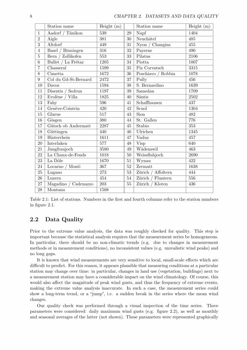
8 CHAPTER 2. DATASETS AND DATA QUALITY

Station name Height (m)1 Aadorf / Tanikon 5392 Aigle 3813 Altdorf 4494 Basel / Binningen 3165 Bern / Zollikofen 5536 Bullet / La Fretaz 12057 Chasseral 15998 Cimetta 16729 Col du Gd-St-Bernard 247210 Davos 159411 Disentis / Sedrun 119712 Evolene / Villa 182513 Fahy 59614 Geneve-Cointrin 42015 Glarus 51716 Gosgen 38017 Gutsch ob Andermatt 228718 Guttingen 44019 Hinterrhein 161120 Interlaken 57721 Jungfraujoch 358022 La Chaux-de-Fonds 101823 La Dole 167024 Locarno / Monti 36725 Lugano 27326 Luzern 45427 Magadino / Cadenazzo 20328 Montana 1508

Station name Height (m)29 Napf 140430 Neuchatel 48531 Nyon / Changins 45532 Payerne 49033 Pilatus 210634 Piotta 100735 Piz Corvatsch 331536 Poschiavo / Robbia 107837 Pully 45638 S. Bernardino 163939 Samedan 170940 Santis 250241 Schaffhausen 43742 Scuol 130443 Sion 48244 St. Gallen 77645 Stabio 35346 Ulrichen 134547 Vaduz 45748 Visp 64049 Wadenswil 46350 Weissfluhjoch 269051 Wynau 42252 Zermatt 163853 Zurich / Affoltern 44454 Zurich / Fluntern 55655 Zurich / Kloten 436

Table 2.1: List of stations. Numbers in the first and fourth columns refer to the station numbersin figure 2.1.

2.2 Data Quality

Prior to the extreme value analysis, the data was roughly checked for quality. This step isimportant because the statistical analysis requires that the measurement series be homogeneous.In particular, there should be no non-climatic trends (e.g. due to changes in measurementmethods or in measurement conditions), no inconsistent values (e.g. unrealistic wind peaks) andno long gaps.

It is known that wind measurements are very sensitive to local, small-scale effects which aredifficult to predict. For this reason, it appears plausible that measuring conditions at a particularstation may change over time: in particular, changes in land use (vegetation, buildings) next toa measurement station may have a considerable impact on the wind climatology. Of course, thiswould also affect the magnitude of peak wind gusts, and thus the frequency of extreme events,making the extreme value analysis inaccurate. In such a case, the measurement series couldshow a long-term trend, or a “jump”, i.e. a sudden break in the series where the mean windchanges.

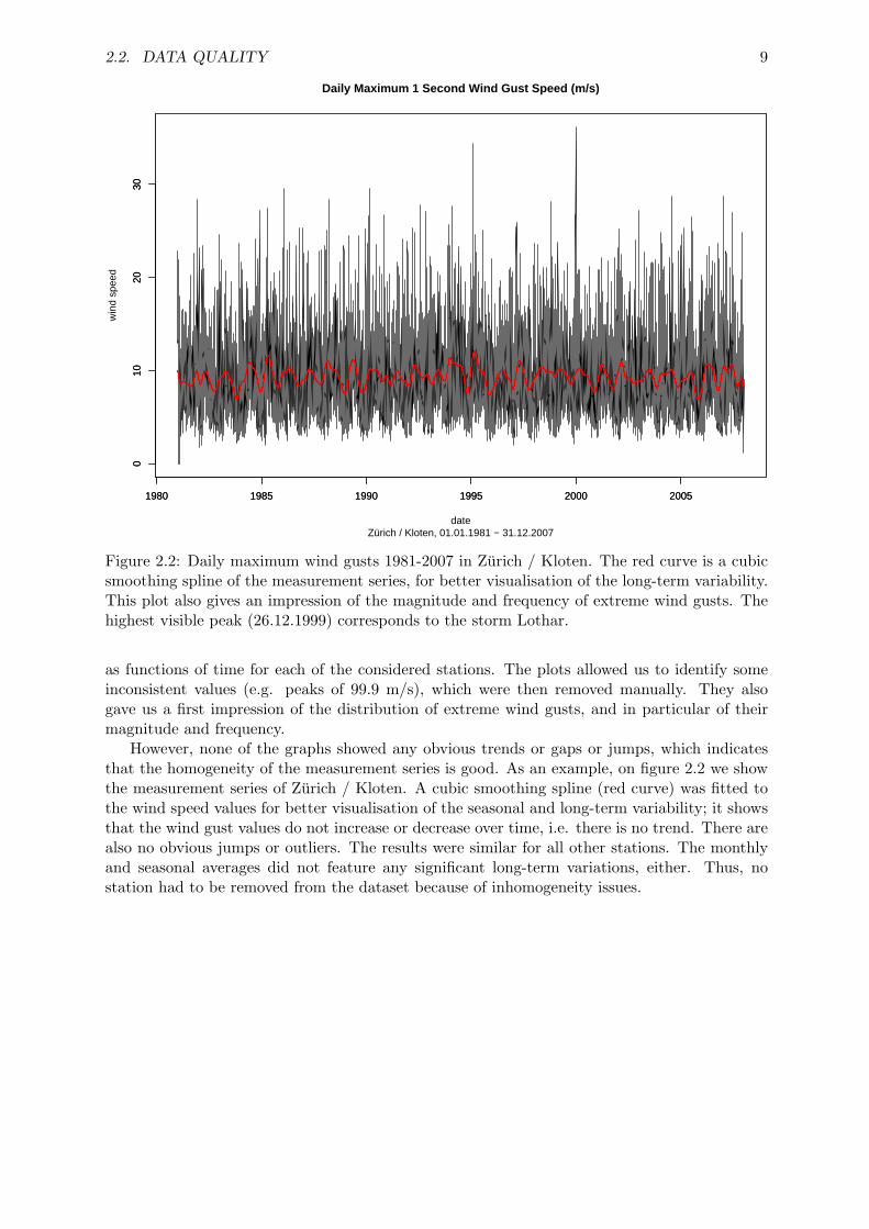
Our quality check was performed through a visual inspection of the time series. Threeparameters were considered: daily maximum wind gusts (e.g. figure 2.2), as well as monthlyand seasonal averages of the latter (not shown). These parameters were represented graphically

2.2. DATA QUALITY 9

010

2030

1980 1985 1990 1995 2000 2005

Daily Maximum 1 Second Wind Gust Speed (m/s)

Zürich / Kloten, 01.01.1981 − 31.12.2007date

win

d sp

eed

010

2030

1980 1985 1990 1995 2000 2005

Figure 2.2: Daily maximum wind gusts 1981-2007 in Zurich / Kloten. The red curve is a cubicsmoothing spline of the measurement series, for better visualisation of the long-term variability.This plot also gives an impression of the magnitude and frequency of extreme wind gusts. Thehighest visible peak (26.12.1999) corresponds to the storm Lothar.

as functions of time for each of the considered stations. The plots allowed us to identify someinconsistent values (e.g. peaks of 99.9 m/s), which were then removed manually. They alsogave us a first impression of the distribution of extreme wind gusts, and in particular of theirmagnitude and frequency.

However, none of the graphs showed any obvious trends or gaps or jumps, which indicatesthat the homogeneity of the measurement series is good. As an example, on figure 2.2 we showthe measurement series of Zurich / Kloten. A cubic smoothing spline (red curve) was fitted tothe wind speed values for better visualisation of the seasonal and long-term variability; it showsthat the wind gust values do not increase or decrease over time, i.e. there is no trend. There arealso no obvious jumps or outliers. The results were similar for all other stations. The monthlyand seasonal averages did not feature any significant long-term variations, either. Thus, nostation had to be removed from the dataset because of inhomogeneity issues.

Chapter 3

Extreme Value Analysis

3.1 Definition

The purpose of extreme value analysis (EVA) is to find reliable estimates of the frequency ofextreme events. In statistical terms, the frequency is usually expressed as a return period (RP)and the value which corresponds to that RP is called the return level (RL). (For some examples,see results in section 4.1.)

It is often the case that when quantifying extremes of any physical process there are limitedobservations of such a process. Usually, from an application point of view, we require informationabout extremes which have not been observed; this requires extrapolation of information fromthe observations at hand. In other words, EVA allows us to estimate RLs even for RPs largerthan the period of observation. The analysis includes uncertainty calculations, with confidenceintervals measuring the accuracy of parameter estimates.

EVA is based on the asymptotic behaviour of observed extremes; for a theoretical definition,see Fisher and Tippett (1928); Coles (2001). Palutikof et al. (1999) review common methodsused to estimate the extreme value distribution of extreme wind speeds.

3.2 The Peak Over Threshold (POT) method

Note: parts of this section were adapted from Della-Marta et al. (2007), section 3.1.The POT approach provides a model for independent exceedances above a large threshold.

Assuming that exceedances are independent, identically distributed random variables, the dis-tribution of exceedances asymptotes to a limit distibution, the Generalised Pareto Distribution(GPD). For more details, see Coles (2001), p. 76.

Thus, the GPD can be used to model exceedances above a given threshold. This distributioncan be written in terms of a generic variable x as:

G (x) = 1 −[1 + ξ(

x − u

σ)]− 1

ξ

(x > u, ξ 6= 0) (3.1)

where u is the selected threshold.The GPD function is a so-called cumulative distribution function, so it can be expressed in

terms of probabilities. Let X be an independent and identically distributed random variable ofthe GPD function. Then equation 3.1 can be rewritten as follows:

Pr(X < x | x > u) = G(x)

Pr(X > x | x > u) = 1 − G(x) (3.2)

Pr(X > x) = Pr(x > u) [1 − G(x)]

10

3.2. THE PEAK OVER THRESHOLD (POT) METHOD 11

a)

0 1 2 3 4 5

01

23

45

6

GPD shape parameter ξ

Exponential Variate V=−log(1−G)

Exc

eeda

nce

Qua

ntile

Y

ξ = 0ξ = −0.2ξ = 0.2σ = 1

b)

0 1 2 3 4 5

02

46

810

12

GPD scale parameter σ

Exponential Variate V=−log(1−G)

Exc

eeda

nce

Qua

ntile

Y

σ = 1σ = 2σ = 4ξ = −0.2

Figure 3.1: Influence of a) the shape parameter ξ and b) the scale parameter σ on the GPDcurve.

Pr (X > x) = ζu

[1 + ξ

(x − u

σ

)]− 1ξ

(3.3)

where ζu = Pr (X > u), i.e. ζu is the probability of the occurrence of an exceedance of a highthreshold, u.

The GPD is characterised by two parameters, ξ the shape parameter and σ the scale param-eter. The shape parameter determines tail behaviour: if ξ > 0 then the maximum of the GPD isunbounded, whereas if ξ < 0 then the tail has a finite extent. If ξ = 0, the GPD reduces to theexponential distribution and is also unbounded in the limit ξ → 0. As for the scale parameter,it measures the scale or “amplitude” of the distribution. The effects of both parameters aredisplayed on figure 3.1.

In this study we are primarily interested in the the N -year return level (RL) xN , which isexceeded once every N years. It can be expressed as

xN = u +σ

ξ

[(Nnyζu)ξ − 1

](3.4)

where ny is the number of observations per year. (For a derivation of this formula, see Coles(2001).) Equation 3.4 suggests that in order to determine the N -year RL three parametersneed to be fitted, ξ, σ and ζu. If we assume that these are rare events, ζu could be expectedto follow a Poisson distribution. Here we deviate slightly from Coles (2001) who suggests ζu

could be modelled by the binomial distribution. The Poisson distribution is characterised bythe parameter λ, the mean number of threshold exceedances per unit time. We can estimateζu ≈ λ/ny and reformulating equation 3.4 in terms of the λ (as also shown by Palutikof et al.,1999) we get:

xN = u +σ

ξ

[(λN)ξ − 1

](3.5)

We estimated ξ and σ in equation 3.5 using maximum likelihood method (Martins andStedinger, 2000; Coles, 2001; details not shown).

12 CHAPTER 3. EXTREME VALUE ANALYSIS

3.3 Declustering and threshold selection

As mentioned in section 3.2, the POT model requires that the exceedances be mutually inde-pendent. However, in the case of wind peaks this assumption may be violated because of serialcorrelation. Indeed, extreme winds over Europe are often associated with mesoscale and syn-optic scale cyclones (Wernli et al., 2002). Typically these systems have a lifetime of around 72hours or less. Since the time resolution of our data is as high as 24 hours, the wind gust peaksare expected to be somewhat dependent.

The most widely adopted method for dealing with this issue is declustering, which filters thedependent observations to obtain a set of threshold excesses that are approximately independent.This is done by defining an empirical rule to identify clusters of exceedances and identifying thecluster maxima; these maxima are called declustered peaks and are assumed to be independent.The declustered peaks are then fitted to the GPD.

Here we use a so-called runs-declustering technique. First, we set a threshold and we defineclusters to be wherever there are consecutive exceedances of this threshold. We then set arun length (minimum separation) between each cluster; a cluster is terminated whenever theseparation between two threshold exceedances is greater than the run length. In our analysiswe chose a minimum separation of five days; this should ensure that the declustered peaksare independent from each other. Other common declustering methods are described in Coles(2001).

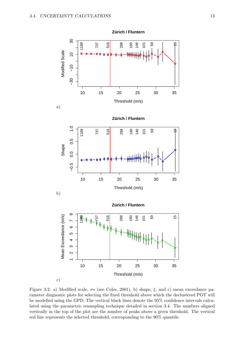
The threshold selection was performed using a number of different diagnostics. The latterare needed to ascertain that the threshold is high enough to be in the asymptotic limit of thedistribution of exceedances. According to the postulates of the GPD, both the modified scaleparameter σ∗ (see Coles, 2001) and the shape parameter should be invariant with thresholdwithin the asymptotic limit. Moreover, the mean of exceedances above a threshold u should bea linear function of u. The three plots in figure 3.2 show the threshold diagnostics for the Zurich/ Fluntern station, following the methods described in Coles (2001). The threshold diagnosticplots show that for most stations, the 90% quantile is an appropriate threshold. This thresholdwas chosen as low as possible to enable as many peaks to be above the threshold and still satisfythe requirements of the GPD.

3.4 Uncertainty calculations

Several methods can be used to estimate confidence intervals. The method we use is profile log-likelihood as it seems to be the most suitable one for extreme wind statistics (Della-Marta et al.,2007). Compared to other uncertainty calculation methods, it has the advantage that it utilisesmore information from the sample, especially the information provided by the most extremeevents. Using this method, it is also possible to obtain asymmetric uncertainty estimates, which,according to Coles (2001), are more precise and should be used in situations where it is necessaryto obtain accurate confidence intervals.

3.4. UNCERTAINTY CALCULATIONS 13

a)

10 15 20 25 30 35

−30

−10

1030

Zürich / Fluntern

Threshold (m/s)

Mod

ified

Sca

le

1189 73

7

516

298

190

146

101 59 15

b)

10 15 20 25 30 35

−0.

50.

00.

51.

0

Zürich / Fluntern

Threshold (m/s)

Sha

pe

1189 73

7

516

298

190

146

101 59 15

c)

10 15 20 25 30 35

12

34

56

78

Zürich / Fluntern

Threshold (m/s)

Mea

n E

xcee

danc

e (m

/s)

1189 737

516

298

190

146

101 59 15

Figure 3.2: a) Modified scale, σ∗ (see Coles, 2001), b) shape, ξ, and c) mean exceedance pa-rameter diagnostic plots for selecting the fixed threshold above which the declustered POT willbe modelled using the GPD. The vertical black lines denote the 95% confidence intervals calcu-lated using the parametric resampling technique detailed in section 3.4. The numbers alignedvertically in the top of the plot are the number of peaks above a given threshold. The verticalred line represents the selected threshold, corresponding to the 90% quantile.

Chapter 4

Results

4.1 Extreme wind distribution at Swiss stations

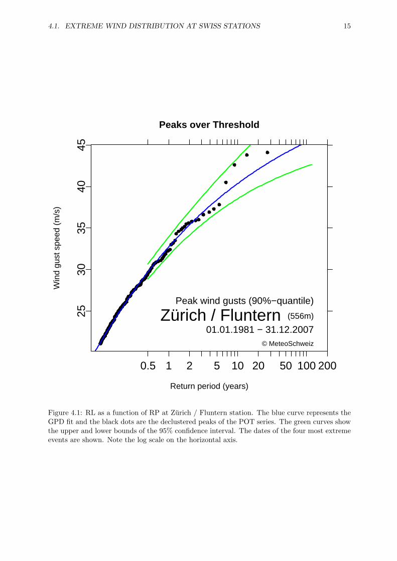
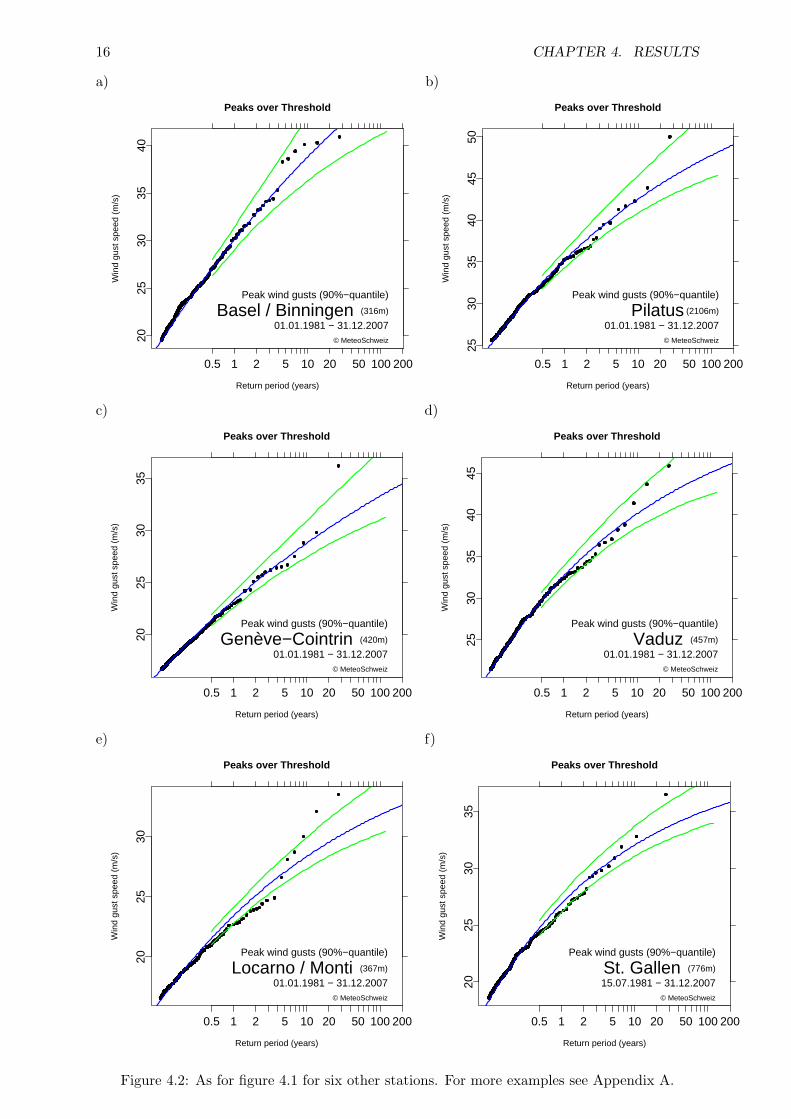
We applied the extreme value analysis methods described in chapter 3 to the declustered POTseries of the 55 stations in our dataset. The results of the GPD fit are represented graphicallywith the return level (RL) as a function of the return period (RP); figures 4.1 and 4.2 show someexamples. The complete extreme wind climatology for all stations is displayed in Appendix Aon figures A.1 to A.9. The RL/RP plots represent the declustered wind peaks above the chosenthreshold together with the GPD fit and the 95% confidence intervals. The confidence intervalsdescribe the uncertainty associated with the parameter estimates. The declustered peaks of thePOT series are also represented as black dots. Note that the x-coordinates of these peaks aredetermined basing only on an empirical estimation of the return period, and not using the fitinformation. We can see that the estimated RPs of the wind peaks feature a very wide range,from approximately 0.1 to >100 years.

One of the striking features of the RL/RP plots is that the shape parameter ξ of the GPD fitis almost always negative. This means that the extreme wind distributions have a finite upperbound (see section 3.2); they do not tend to infinity. In section 4.2 the spatial distribution ofthe GPD parameters is analysed in more detail.

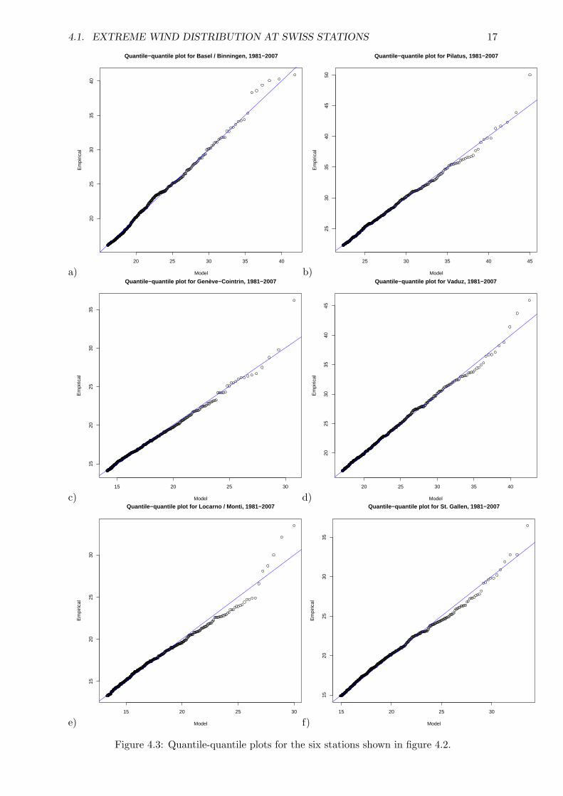
The results show that in most cases the GPD fit of the time series is good; this is confirmedby the quantile-quantile plots (see figure 4.3 a) - d)). However, at some stations (about ten)the empirical values show systematic deviation from modelled values (figure 4.3 e) - f)). Thedeviations are particularly large at Ticino stations; as an example, we show the model fit forLocarno / Monti (figure 4.3 e)). Here a large part of the observed peaks are systematicallybelow the model fit. Such systematic deviations also happen for different threshold values, sothe selected threshold does not seem to be the cause of the problem. Nevertheless, we decided tokeep the concerned stations in our analysis, since the deviation from the model does not appearcritical at any of these stations.

14

4.1. EXTREME WIND DISTRIBUTION AT SWISS STATIONS 15

Peaks over Threshold

Return period (years)

Win

d gu

st s

peed

(m

/s)

Peak wind gusts (90%−quantile)

Zürich / Fluntern (556m)

01.01.1981 − 31.12.2007© MeteoSchweiz

0.5 1 2 5 10 20 50 100 200

2530

3540

45

Figure 4.1: RL as a function of RP at Zurich / Fluntern station. The blue curve represents theGPD fit and the black dots are the declustered peaks of the POT series. The green curves showthe upper and lower bounds of the 95% confidence interval. The dates of the four most extremeevents are shown. Note the log scale on the horizontal axis.

16 CHAPTER 4. RESULTS

a)



Win

d gu

st s

peed

(m

/s)


Basel / Binningen (316m)

01.01.1981 − 31.12.2007© MeteoSchweiz

0.5 1 2 5 10 20 50 100 200

2025

3035

40

b)



Win

d gu

st s

peed

(m

/s)


Pilatus (2106m)

01.01.1981 − 31.12.2007© MeteoSchweiz

0.5 1 2 5 10 20 50 100 200

2530

3540

4550

c)



Win

d gu

st s

peed

(m

/s)


Genève−Cointrin (420m)

01.01.1981 − 31.12.2007© MeteoSchweiz

0.5 1 2 5 10 20 50 100 200

2025

3035

d)



Win

d gu

st s

peed

(m

/s)


Vaduz (457m)

01.01.1981 − 31.12.2007© MeteoSchweiz

0.5 1 2 5 10 20 50 100 200

2530

3540

45

e)



Win

d gu

st s

peed

(m

/s)


Locarno / Monti (367m)

01.01.1981 − 31.12.2007© MeteoSchweiz

0.5 1 2 5 10 20 50 100 200

2025

30

f)



Win

d gu

st s

peed

(m

/s)


St. Gallen (776m)

15.07.1981 − 31.12.2007© MeteoSchweiz

0.5 1 2 5 10 20 50 100 200

2025

3035

Figure 4.2: As for figure 4.1 for six other stations. For more examples see Appendix A.

4.1. EXTREME WIND DISTRIBUTION AT SWISS STATIONS 17

a)20 25 30 35 40

2025

3035

40

Model

Em

piric

al

Quantile−quantile plot for Basel / Binningen, 1981−2007

b)25 30 35 40 45

2530

3540

4550

Model

Em

piric

al

Quantile−quantile plot for Pilatus, 1981−2007

c)15 20 25 30

1520

2530

35

Model

Em

piric

al

Quantile−quantile plot for Genève−Cointrin, 1981−2007

d)20 25 30 35 40

2025

3035

4045

Model

Em

piric

al

Quantile−quantile plot for Vaduz, 1981−2007

e)15 20 25 30

1520

2530

Model

Em

piric

al

Quantile−quantile plot for Locarno / Monti, 1981−2007

f)15 20 25 30

1520

2530

35

Model

Em

piric

al

Quantile−quantile plot for St. Gallen, 1981−2007

Figure 4.3: Quantile-quantile plots for the six stations shown in figure 4.2.


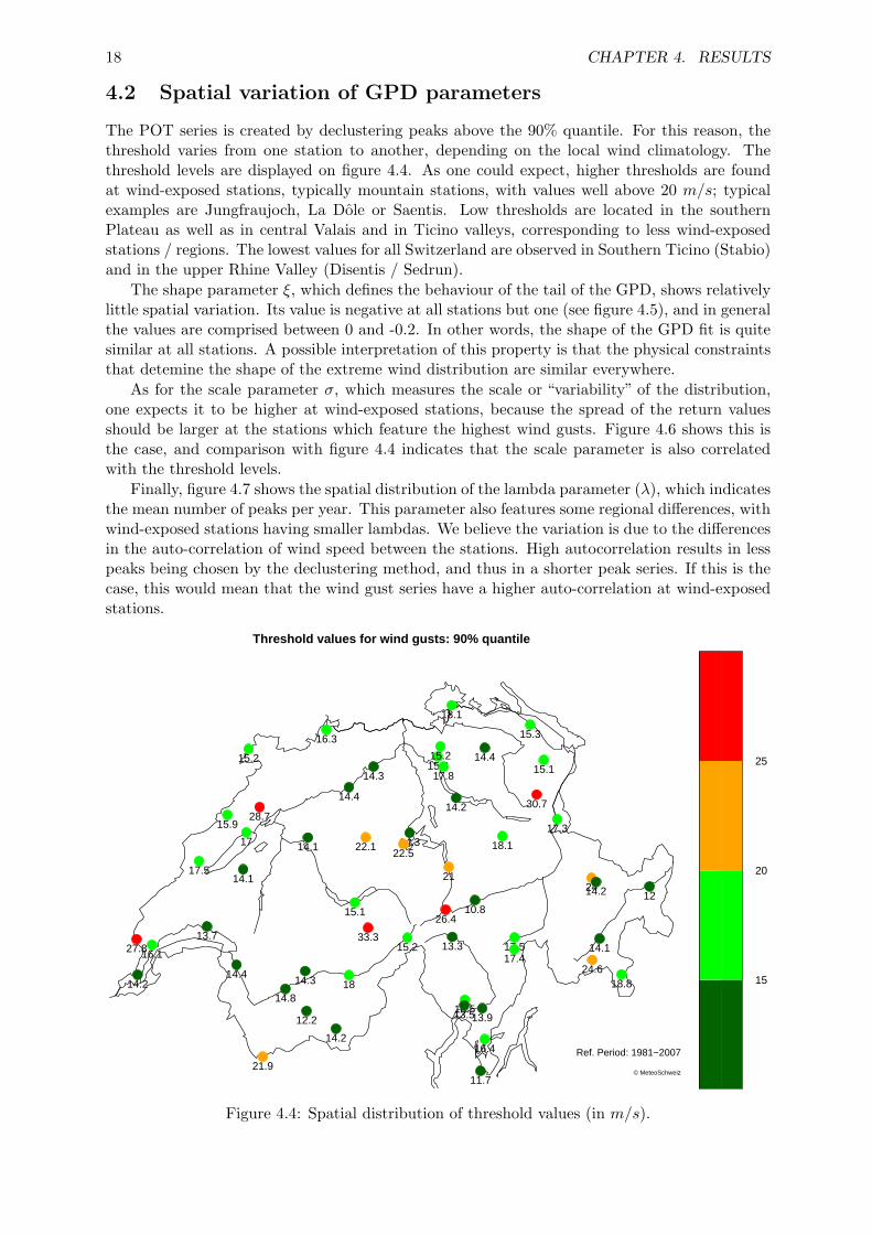
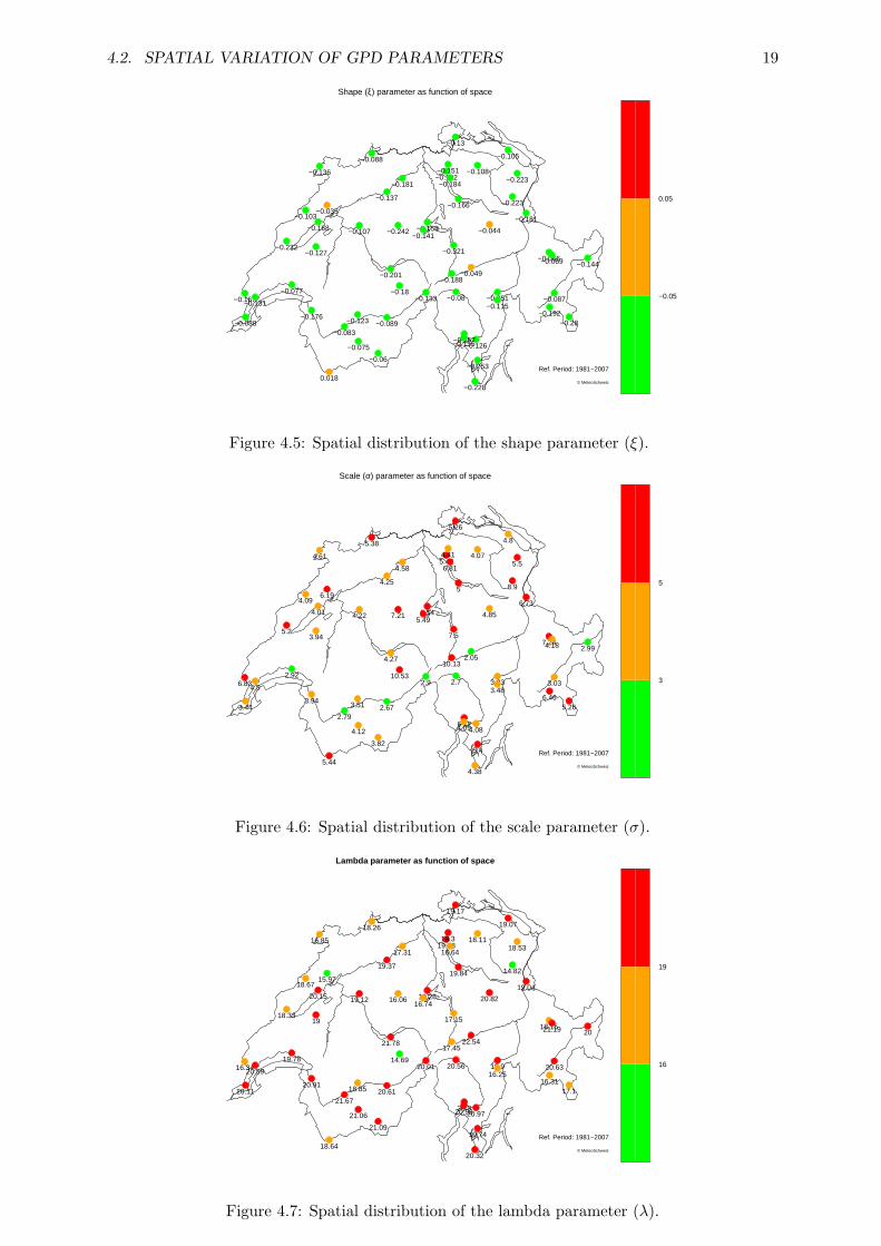
4.2 Spatial variation of GPD parameters

The POT series is created by declustering peaks above the 90% quantile. For this reason, thethreshold varies from one station to another, depending on the local wind climatology. Thethreshold levels are displayed on figure 4.4. As one could expect, higher thresholds are foundat wind-exposed stations, typically mountain stations, with values well above 20 m/s; typicalexamples are Jungfraujoch, La Dole or Saentis. Low thresholds are located in the southernPlateau as well as in central Valais and in Ticino valleys, corresponding to less wind-exposedstations / regions. The lowest values for all Switzerland are observed in Southern Ticino (Stabio)and in the upper Rhine Valley (Disentis / Sedrun).

The shape parameter ξ, which defines the behaviour of the tail of the GPD, shows relativelylittle spatial variation. Its value is negative at all stations but one (see figure 4.5), and in generalthe values are comprised between 0 and -0.2. In other words, the shape of the GPD fit is quitesimilar at all stations. A possible interpretation of this property is that the physical constraintsthat detemine the shape of the extreme wind distribution are similar everywhere.

As for the scale parameter σ, which measures the scale or “variability” of the distribution,one expects it to be higher at wind-exposed stations, because the spread of the return valuesshould be larger at the stations which feature the highest wind gusts. Figure 4.6 shows this isthe case, and comparison with figure 4.4 indicates that the scale parameter is also correlatedwith the threshold levels.

Finally, figure 4.7 shows the spatial distribution of the lambda parameter (λ), which indicatesthe mean number of peaks per year. This parameter also features some regional differences, withwind-exposed stations having smaller lambdas. We believe the variation is due to the differencesin the auto-correlation of wind speed between the stations. High autocorrelation results in lesspeaks being chosen by the declustering method, and thus in a shorter peak series. If this is thecase, this would mean that the wind gust series have a higher auto-correlation at wind-exposedstations.

15

20

25

10.8

17.5

2414.2

17.3

15.1

15.3

18.1

16.3

30.7

14.415.315.2

18.1

14.2

17.8

26.4

21

14.322.5

33.3

15.1

14.1

14.117.5

17

28.7

22.1

14.4

14.3

15.2

14.2

1814.3

12.2

14.8

21.9

14.4

13.727.816.1

14.2

15.9

15.2

13.317.4

13.918.513.5

16.4

11.7

18.824.6

14.1

12

© MeteoSchweiz

Ref. Period: 1981−2007

Threshold values for wind gusts: 90% quantile

Figure 4.4: Spatial distribution of threshold values (in m/s).

4.2. SPATIAL VARIATION OF GPD PARAMETERS 19

−0.05

0.05

−0.049

−0.051

−0.066−0.069

−0.181

−0.223

−0.105

−0.13

−0.088

−0.223

−0.108−0.192−0.151

−0.044

−0.166

−0.184

−0.188

−0.321

−0.158−0.141

−0.18

−0.201

−0.107

−0.127−0.232

−0.168

−0.035

−0.242

−0.137

−0.181

−0.133

−0.06

−0.089−0.123

−0.075

−0.083

0.018

−0.176

−0.077−0.167−0.131

−0.088

−0.103

−0.136

−0.08−0.115

−0.126−0.257−0.155

−0.253

−0.228

−0.28−0.192

−0.087

−0.144

© MeteoSchweiz


Shape (ξ) parameter as function of space

Figure 4.5: Spatial distribution of the shape parameter (ξ).

3

5

2.05

3.83

7.244.18

6.73

5.5

4.8

5.26

5.38

8.9

4.075.424.41

4.85

5

6.81

10.13

7.5

5.545.49

10.53

4.27

4.22

3.945.2

4.01

6.19

7.21

4.25

4.58

2.9

3.82

2.673.51

4.12

2.79

5.44

3.94

2.926.834.5

3.44

4.09

4.61

2.73.48

4.086.124.09

5.4

4.38

5.266.46

3.03

2.99

© MeteoSchweiz


Scale (σ) parameter as function of space

Figure 4.6: Spatial distribution of the scale parameter (σ).

16

19

22.54

19.9

18.1521.19

19.04

18.53

19.07

19.17

18.26

14.82

18.1119.0819.3

20.82

19.84

16.64

17.45

17.15

19.2816.74

14.69

21.78

19.12

1918.33

20.15

15.97

16.06

19.37

17.31

20.01

21.09

20.6118.85

21.06

21.67

18.64

20.91

19.7816.3420.59

20.11

18.67

16.85

20.5616.25

20.9720.320.98

19.74

20.32

17.116.31

20.63

20

© MeteoSchweiz


Lambda parameter as function of space

Figure 4.7: Spatial distribution of the lambda parameter (λ).


4.3 Return levels and return periods

4.3.1 Return periods of given wind speeds

An interesting application of our results lies in the possibility of estimating the return periodof any given wind gust speed. Of course, these estimates are associated with uncertainties, butfor not too extreme wind gust speeds the confidence intervals are reasonably small. Because ofthese uncertainties we only display ranges of RP values and not the exact values; the ranges arerepresented with a colour code. We chose to investigate the return period of wind gusts of 25,30 and 35 m/s (90, 108 and 126 km/h respectively). The results are shown on figure 4.8.

The plots indicate that the distribution of extreme winds is very inhomogeneous, since thereturn periods range from <2 to 100+ years. We see that for most stations, wind gusts of 25 m/sare not exceptional, with most return periods being lower than 2 years. The frequency of gustsof 30 m/s, however, is very variable. Wind-exposed stations can be easily identified because ofthe low return periods; as could be expected, the highest return periods are situated in regionsthat are protected from high wind speeds, such as some inner alpine valleys. Finally, wind gustsof 35 m/s are extreme events almost everywhere, except for very wind-exposed stations. Noticethat a few stations in the northern Swiss plateau feature relatively low return periods (<5 years),namely Zurich / Fluntern, Schaffhausen and Basel / Binningen; this is also the case for stationsin Fohn valleys, such as Altdorf and Vaduz.

4.3.2 Return levels of given return periods

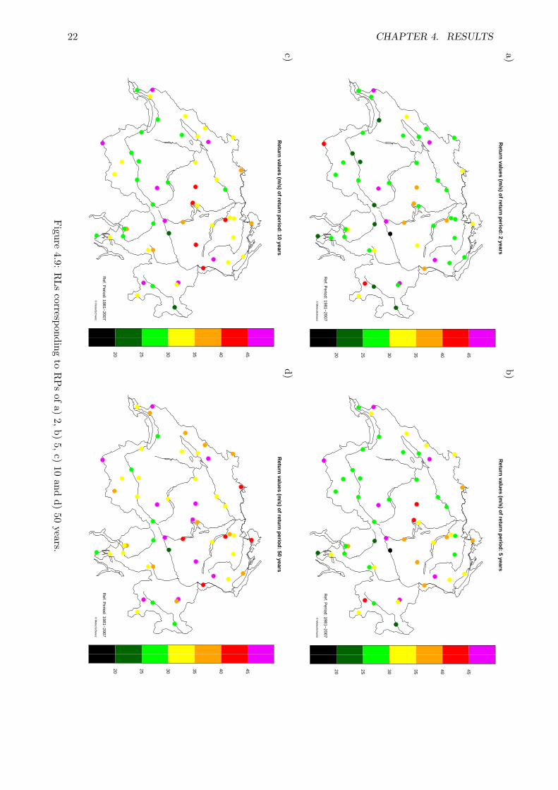
In this section we analyse the spatial variability of the return levels (RLs) of given return periods(RPs); for this we consider RPs of 2, 5, 10 and 50 years (see figure 4.9). As in previous plots, wecan notice here again the differences in wind exposure: the most wind-exposed stations have thehighest return levels. In the following we make a few comments on figures 4.9 b) and d). We cansee that the 5-year return levels for most lowland stations on the Swiss Plateau and in Valaisare comprised between 25 and 30 m/s. The 50-year return levels are more heterogeneous, withvalues generally between 30 and 40 m/s. Note that the uncertainty (and thus the confidenceintervals) of the RL estimates increase with the RP; in particular, a RP of 50 years, whichcorresponds to a very extreme event, is associated with very large confidence intervals. For thisreason, the RL estimates should be interpreted with caution.

4.3. RETURN LEVELS AND RETURN PERIODS 21

a)

2

5

10

20

50

100

© MeteoSchweiz


Return period (years) of wind gusts: 25 m/s

b)

2

5

10

20

50

100

© MeteoSchweiz



c)

2

5

10

20

50

100

© MeteoSchweiz



Figure 4.8: Return period of wind gusts of a) 25, b) 30 and c) 35 m/s.

22 CHAPTER 4. RESULTSa)

20 25 30 35 40 45

© M

eteoSchw

eiz

Ref. P

eriod: 1981−2007

Retu

rn valu

es (m/s) o

f return

perio

d: 2 years

b)

20 25 30 35 40 45

© M

eteoSchw

eiz

Ref. P

eriod: 1981−2007

Retu

rn valu

es (m/s) o

f return

perio

d: 5 years

c)

20 25 30 35 40 45

© M

eteoSchw

eiz

Ref. P

eriod: 1981−2007

Retu

rn valu

es (m/s) o

f return

perio

d: 10 years

d)

20 25 30 35 40 45

© M

eteoSchw

eiz

Ref. P

eriod: 1981−2007

Retu

rn valu

es (m/s) o

f return

perio

d: 50 years

Figure

4.9:R

Ls

correspondingto

RP

sof

a)2,

b)5,

c)10

andd)

50years.

4.4. RETURN PERIOD OF SOME PROMINENT WIND STORMS 23

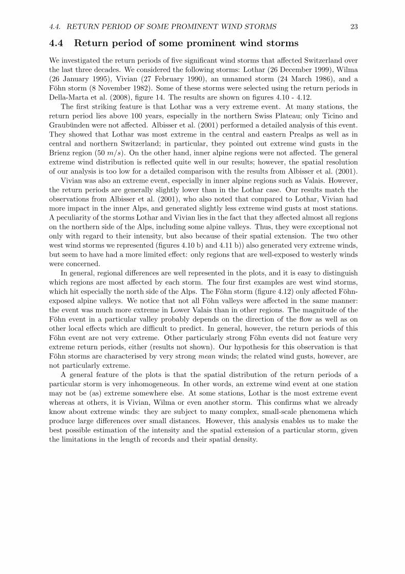
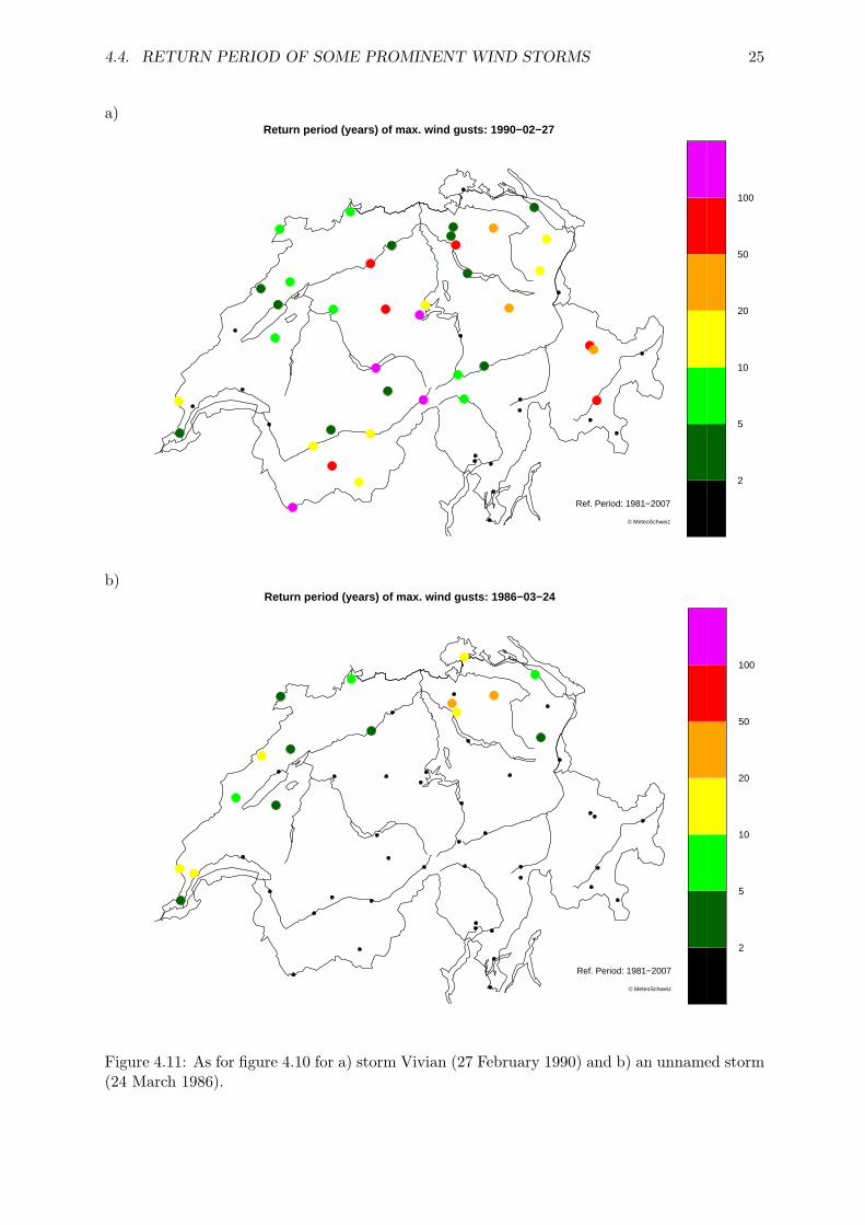
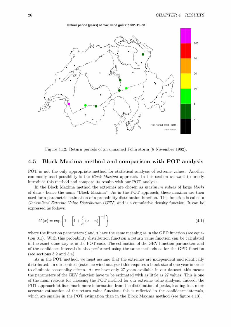
4.4 Return period of some prominent wind storms

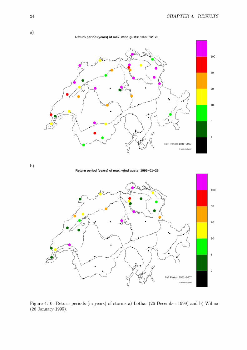
We investigated the return periods of five significant wind storms that affected Switzerland overthe last three decades. We considered the following storms: Lothar (26 December 1999), Wilma(26 January 1995), Vivian (27 February 1990), an unnamed storm (24 March 1986), and aFohn storm (8 November 1982). Some of these storms were selected using the return periods inDella-Marta et al. (2008), figure 14. The results are shown on figures 4.10 - 4.12.

The first striking feature is that Lothar was a very extreme event. At many stations, thereturn period lies above 100 years, especially in the northern Swiss Plateau; only Ticino andGraubunden were not affected. Albisser et al. (2001) performed a detailed analysis of this event.They showed that Lothar was most extreme in the central and eastern Prealps as well as incentral and northern Switzerland; in particular, they pointed out extreme wind gusts in theBrienz region (50 m/s). On the other hand, inner alpine regions were not affected. The generalextreme wind distribution is reflected quite well in our results; however, the spatial resolutionof our analysis is too low for a detailed comparison with the results from Albisser et al. (2001).

Vivian was also an extreme event, especially in inner alpine regions such as Valais. However,the return periods are generally slightly lower than in the Lothar case. Our results match theobservations from Albisser et al. (2001), who also noted that compared to Lothar, Vivian hadmore impact in the inner Alps, and generated slightly less extreme wind gusts at most stations.A peculiarity of the storms Lothar and Vivian lies in the fact that they affected almost all regionson the northern side of the Alps, including some alpine valleys. Thus, they were exceptional notonly with regard to their intensity, but also because of their spatial extension. The two otherwest wind storms we represented (figures 4.10 b) and 4.11 b)) also generated very extreme winds,but seem to have had a more limited effect: only regions that are well-exposed to westerly windswere concerned.

In general, regional differences are well represented in the plots, and it is easy to distinguishwhich regions are most affected by each storm. The four first examples are west wind storms,which hit especially the north side of the Alps. The Fohn storm (figure 4.12) only affected Fohn-exposed alpine valleys. We notice that not all Fohn valleys were affected in the same manner:the event was much more extreme in Lower Valais than in other regions. The magnitude of theFohn event in a particular valley probably depends on the direction of the flow as well as onother local effects which are difficult to predict. In general, however, the return periods of thisFohn event are not very extreme. Other particularly strong Fohn events did not feature veryextreme return periods, either (results not shown). Our hypothesis for this observation is thatFohn storms are characterised by very strong mean winds; the related wind gusts, however, arenot particularly extreme.

A general feature of the plots is that the spatial distribution of the return periods of aparticular storm is very inhomogeneous. In other words, an extreme wind event at one stationmay not be (as) extreme somewhere else. At some stations, Lothar is the most extreme eventwhereas at others, it is Vivian, Wilma or even another storm. This confirms what we alreadyknow about extreme winds: they are subject to many complex, small-scale phenomena whichproduce large differences over small distances. However, this analysis enables us to make thebest possible estimation of the intensity and the spatial extension of a particular storm, giventhe limitations in the length of records and their spatial density.


a)

2

5

10

20

50

100

© MeteoSchweiz


Return period (years) of max. wind gusts: 1999−12−26

b)

2

5

10

20

50

100

© MeteoSchweiz



Figure 4.10: Return periods (in years) of storms a) Lothar (26 December 1999) and b) Wilma(26 January 1995).

4.4. RETURN PERIOD OF SOME PROMINENT WIND STORMS 25

a)

2

5

10

20

50

100

© MeteoSchweiz



b)

2

5

10

20

50

100

© MeteoSchweiz



Figure 4.11: As for figure 4.10 for a) storm Vivian (27 February 1990) and b) an unnamed storm(24 March 1986).


2

5

10

20

50

100

© MeteoSchweiz



Figure 4.12: Return periods of an unnamed Fohn storm (8 November 1982).

4.5 Block Maxima method and comparison with POT analysis

POT is not the only appropriate method for statistical analysis of extreme values. Anothercommonly used possibility is the Block Maxima approach. In this section we want to brieflyintroduce this method and compare its results with our POT analysis.

In the Block Maxima method the extremes are chosen as maximum values of large blocksof data - hence the name “Block Maxima”. As in the POT approach, these maxima are thenused for a parametric estimation of a probability distribution function. This function is called aGeneralised Extreme Value Distribution (GEV) and is a cumulative density function. It can beexpressed as follows:

G (x) = exp

{1 −

[1 +

ξ

σ(x − u)

]− 1ξ

}(4.1)

where the function parameters ξ and σ have the same meaning as in the GPD function (see equa-tion 3.1). With this probability distribution function a return value function can be calculatedin the exact same way as in the POT case. The estimation of the GEV function parameters andof the confidence intervals is also performed using the same methods as for the GPD function(see sections 3.2 and 3.4).

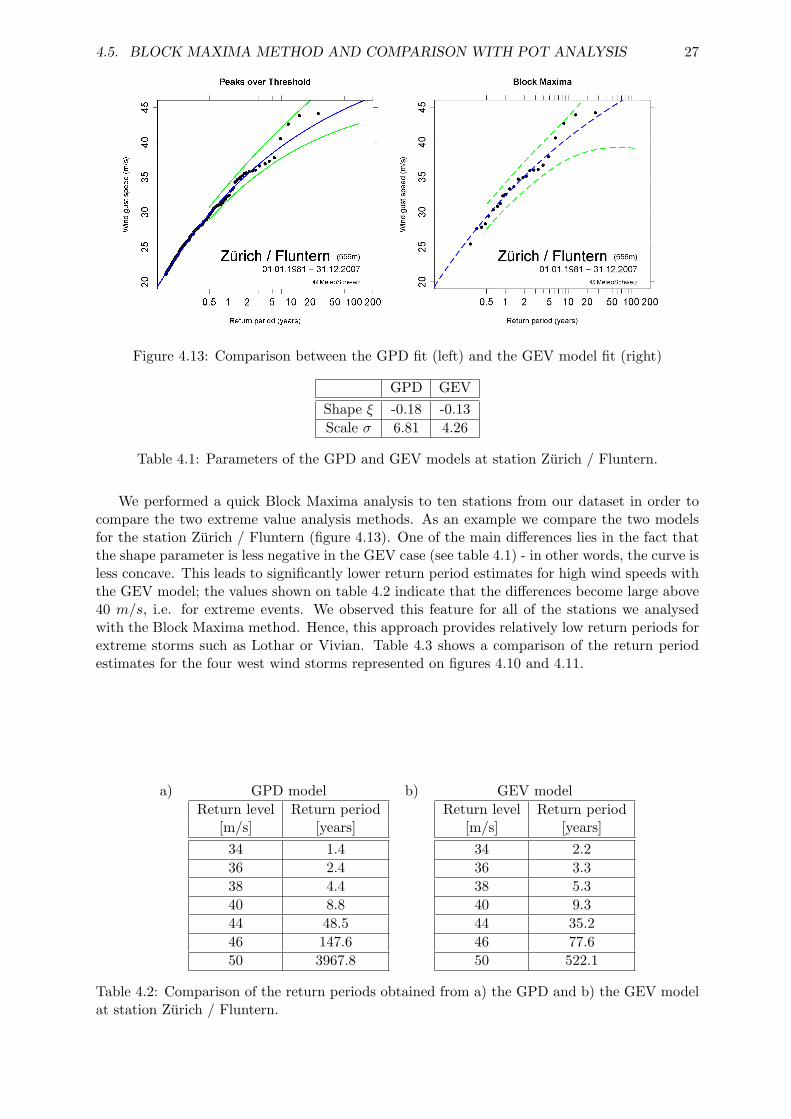
As in the POT method, we must assume that the extremes are independent and identicallydistributed. In our context (extreme wind analysis) this requires a block size of one year in orderto eliminate seasonality effects. As we have only 27 years available in our dataset, this meansthe parameters of the GEV function have to be estimated with as little as 27 values. This is oneof the main reasons for choosing the POT method for our extreme value analysis. Indeed, thePOT approach utilises much more information from the distribution of peaks, leading to a moreaccurate estimation of the return value function; this is reflected in the confidence intervals,which are smaller in the POT estimation than in the Block Maxima method (see figure 4.13).

4.5. BLOCK MAXIMA METHOD AND COMPARISON WITH POT ANALYSIS 27

Figure 4.13: Comparison between the GPD fit (left) and the GEV model fit (right)

GPD GEVShape ξ -0.18 -0.13Scale σ 6.81 4.26

Table 4.1: Parameters of the GPD and GEV models at station Zurich / Fluntern.

We performed a quick Block Maxima analysis to ten stations from our dataset in order tocompare the two extreme value analysis methods. As an example we compare the two modelsfor the station Zurich / Fluntern (figure 4.13). One of the main differences lies in the fact thatthe shape parameter is less negative in the GEV case (see table 4.1) - in other words, the curve isless concave. This leads to significantly lower return period estimates for high wind speeds withthe GEV model; the values shown on table 4.2 indicate that the differences become large above40 m/s, i.e. for extreme events. We observed this feature for all of the stations we analysedwith the Block Maxima method. Hence, this approach provides relatively low return periods forextreme storms such as Lothar or Vivian. Table 4.3 shows a comparison of the return periodestimates for the four west wind storms represented on figures 4.10 and 4.11.

a) GPD model b) GEV modelReturn level Return period

[m/s] [years]34 1.436 2.438 4.440 8.844 48.546 147.650 3967.8

Return level Return period[m/s] [years]34 2.236 3.338 5.340 9.344 35.246 77.650 522.1

Table 4.2: Comparison of the return periods obtained from a) the GPD and b) the GEV modelat station Zurich / Fluntern.


GPD model GEV modelStorm name Max. wind gust Return period Max. wind gust Return period

and date speed [m/s] [years] speed [m/s] [years]Lothar 43.8 43.9 43.8 32.7

26.12.1999Wilma 35.8 2.3 35.8 3.1

26.01.1995Vivian 44.1 51.0 44.1 36.6

27.02.1990unnamed 40.5 10.6 40.5 10.824.03.1986

Table 4.3: As in table 4.2 for the four storms displayed on figures 4.10 and 4.11.

In their analysis of the Lothar event, Albisser et al. (2001) also performed a Block Maximaanalysis for 28 stations. For Zurich / Fluntern their estimated return period was as low as12 years. However, their analysis was based on only 19 years of measurement records; thismight explain the difference compared to our results. This seems to indicate that for too shortmeasurement series the Block Maxima method overestimates the shape parameter, so that italso underestimates the return periods of extreme events. If this is the case, the two approaches(Block Maxima and POT) should give quite similar results for longer time series.

Chapter 5

Discussion and Recommendationsfor Further Research

5.1 Discussion of the results

One of the main goals of this work was to assess the potential for creating a wind climatologybased on in-situ wind gust measurements. Our results have shown that the data quality of mostof the time series is very good and that the distribution of the POT series can be modelled wellby a GPD model fit. In particular, the quality and length of the data are sufficiently good for anextreme value analysis; the quantile-quantile plots show the model fit was good, with systematicdeviations in a few cases only. In other words, it is possible to obtain reliable station-basedextreme wind climatologies.

Compared to other studies based on reanalysis model data (Della-Marta et al., 2007, 2008),the advantage of using station data lies in the fact that small-scale effects acting on surfacewinds can be much better described. Indeed, global reanalysis data for surface wind have biasesand are very coarse in resolution; they are thus not be suitable for wind analysis at local spacescales.

Our analysis provides information about the RP of local wind gusts at a particular station.However, visual representation of the spatial distribution of the RPs also gives a more generalpicture about the magnitude of an extreme wind event on a regional scale, and describes howthe effects of the storm are distributed in space. Thus, the analysis of storm Lothar showed notonly that the intensity of the local wind gusts was extreme, but also that the spatial extensionof the extreme gusts was exceptional; the storm was extreme not only at a specific point, butover all of the north side of the Alps. This corresponds well with the analysis made by Albisseret al. (2001).

In the following we want to compare briefly our results with the work done by Della-Martaet al. (2008) based on reanalysis model data. Their parameter estimates were similar to ours,especially with respect to the shape parameter (ξ), with negative values almost everywhere; onlya few grid points had slightly positive values. In particular, their wind climatologies over landexhibit shape values in the range -0.33 ≤ ξ ≤ -0.18, which means that their grid point basedGPD fits also had an upper bound. In addition, the distribution of the scale parameter (σ)was similar to that of the threshold levels, grid points with high thresholds displaying widerdistributions; this also reflects our results. The lambda parameters cannot be compared becauseof different time block sizes.

Regarding the RP of specific storms, we also see a good correspondence between the resultsof the two studies. Their grid point based RP estimates for Lothar also display values close to orabove 100 years over much of central Europe. Wind gust analysis of storm Vivian shows RPs inthe same order of magnitude as ours as well. However, it is difficult to make a direct comparisonbetween the two studies, since the resolution of the analysis in Della-Marta et al. (2008) is muchcoarser than ours, so that no accurate RP estimation can be made for Switzerland.

29

30CHAPTER 5. DISCUSSION AND RECOMMENDATIONS FOR FURTHER RESEARCH

5.2 Recommendations for further research

Due to the requirements of this Bachelor thesis, we had to restrict our EVA to 55 stations withfull time series (1981 - 2007). Indeed, the check of the quality and homogeneity of the series was atime consuming step. However, we believe it is necessary to include further stations with shortermeasurement series, as 132 stations are available in total. This would provide a better spatialresolution, giving even more information about local differences in extreme wind climatologiestogether with more reliable RP estimates.

Another possibility lies in the inspection of the quality of the time series. We limited ourselvesto analysing the long-term variability of the measurement series, as well as monthly and seasonalaverages of the latter. A deeper analysis would be beneficial, as we think quality issues mightbe the cause for some of the bad GPD fits at certain stations.

The systematic deviations from the GPD fit should also be inspected carefully. We mentionedthat all lowland stations in Ticino exhibited this feature. However, we only have four lowlandstations in this region, so it would be necessary to include more Ticino stations into the analysis.A question that should be addressed is whether the deviations are due to data quality issues orwhether other factors play a role, e.g. climatological factors that might influence the distributionof extreme winds.

Finally, in the extreme value analysis of the wind gusts, the synoptic weather pattern couldalso be taken into account. Indeed, our analysis is independent from the wind direction. It isknown that most extreme wind events - at least on a regional scale - are related to west windstorms (mostly in winter). We believe it might be interesting to take the wind direction intoaccount as this would enable to evaluate the extremeness of other situations, such as Bise winds,independently from the general wind climatology. This would also make it possible to estimatewhich regions are most affected by each type of general weather pattern.

Appendix A

Extreme wind climatologies



Win

d gu

st s

peed

(m

/s)


Disentis / Sedrun (1197m)

01.01.1981 − 31.12.2007© MeteoSchweiz

0.5 1 2 5 10 20 50 100 200

1214

1618

2022

2426



Win

d gu

st s

peed

(m

/s)


Hinterrhein (1611m)

01.01.1981 − 31.12.2007© MeteoSchweiz

0.5 1 2 5 10 20 50 100 200

2025

3035

40



Win

d gu

st s

peed

(m

/s)


Weissfluhjoch (2690m)

01.01.1981 − 31.12.2007© MeteoSchweiz

0.5 1 2 5 10 20 50 100 200

3040

5060



Win

d gu

st s

peed

(m

/s)


Davos (1594m)

01.01.1981 − 31.12.2007© MeteoSchweiz

0.5 1 2 5 10 20 50 100 200

2025

3035

Figure A.1: Extreme wind climatologies. For description see figure 4.1.

31

32 APPENDIX A. EXTREME WIND CLIMATOLOGIES



Win

d gu

st s

peed

(m

/s)


Güttingen (440m)

01.01.1981 − 31.12.2007© MeteoSchweiz

0.5 1 2 5 10 20 50 100 200

2025

3035



Win

d gu

st s

peed

(m

/s)


Schaffhausen (437m)

23.06.1981 − 31.12.2007© MeteoSchweiz

0.5 1 2 5 10 20 50 100 200

2530

3540

45



Win

d gu

st s

peed

(m

/s)


Säntis (2502m)

01.01.1981 − 31.12.2007© MeteoSchweiz

0.5 1 2 5 10 20 50 100 200

3540

4550

5560



Win

d gu

st s

peed

(m

/s)


Aadorf / Tänikon (539m)

01.01.1981 − 31.12.2007© MeteoSchweiz

0.5 1 2 5 10 20 50 100 200

2025

30



Win

d gu

st s

peed

(m

/s)


Zürich / Affoltern (444m)

01.01.1981 − 31.12.2007© MeteoSchweiz

0.5 1 2 5 10 20 50 100 200

2025

3035



Win

d gu

st s

peed

(m

/s)


Zürich / Kloten (436m)

01.01.1981 − 31.12.2007© MeteoSchweiz

0.5 1 2 5 10 20 50 100 200

2025

3035


33



Win

d gu

st s

peed

(m

/s)


Glarus (517m)

01.01.1981 − 31.12.2007© MeteoSchweiz

0.5 1 2 5 10 20 50 100 200

2530

3540

4550



Win

d gu

st s

peed

(m

/s)


Wädenswil (485m)

01.01.1981 − 31.12.2007© MeteoSchweiz

0.5 1 2 5 10 20 50 100 200

2025

3035



Win

d gu

st s

peed

(m

/s)


Gütsch ob Andermatt (2287m)

01.01.1981 − 31.12.2007© MeteoSchweiz

0.5 1 2 5 10 20 50 100 200

3540

4550

5560



Win

d gu

st s

peed

(m

/s)


Altdorf (449m)

01.01.1981 − 31.12.2007© MeteoSchweiz

0.5 1 2 5 10 20 50 100 200

2530

3540



Win

d gu

st s

peed

(m

/s)


Luzern (454m)

01.01.1981 − 31.12.2007© MeteoSchweiz

0.5 1 2 5 10 20 50 100 200

2025

3035

40



Win

d gu

st s

peed

(m

/s)


Jungfraujoch (3580m)

20.08.1981 − 31.12.2007© MeteoSchweiz

0.5 1 2 5 10 20 50 100 200

4050

6070





Win

d gu

st s

peed

(m

/s)


Interlaken (577m)

01.01.1981 − 31.12.2007© MeteoSchweiz

0.5 1 2 5 10 20 50 100 200

1820

2224

2628

3032



Win

d gu

st s

peed

(m

/s)


Bern / Zollikofen (553m)

01.01.1981 − 31.12.2007© MeteoSchweiz

0.5 1 2 5 10 20 50 100 200

2025

3035



Win

d gu

st s

peed

(m

/s)


Payerne (490m)

01.01.1981 − 31.12.2007© MeteoSchweiz

0.5 1 2 5 10 20 50 100 200

2025

30



Win

d gu

st s

peed

(m

/s)


Bullet / La Frétaz (1205m)

01.01.1981 − 31.12.2007© MeteoSchweiz

0.5 1 2 5 10 20 50 100 200

2025

3035



Win

d gu

st s

peed

(m

/s)


Neuchâtel (485m)

01.01.1981 − 31.12.2007© MeteoSchweiz

0.5 1 2 5 10 20 50 100 200

2022

2426

2830

3234



Win

d gu

st s

peed

(m

/s)


Chasseral (1599m)

17.02.1981 − 31.12.2007© MeteoSchweiz

0.5 1 2 5 10 20 50 100 200

3540

4550

5560


35



Win

d gu

st s

peed

(m

/s)


Napf (1404m)

01.01.1981 − 31.12.2007© MeteoSchweiz

0.5 1 2 5 10 20 50 100 200

2530

3540

45



Win

d gu

st s

peed

(m

/s)


Wynau (422m)

01.01.1981 − 31.12.2007© MeteoSchweiz

0.5 1 2 5 10 20 50 100 200

2025

30



Win

d gu

st s

peed

(m

/s)


Gösgen (380m)

03.11.1981 − 31.12.2007© MeteoSchweiz

0.5 1 2 5 10 20 50 100 200

2025

30



Win

d gu

st s

peed

(m

/s)


Ulrichen (1346m)

01.01.1981 − 31.12.2007© MeteoSchweiz

0.5 1 2 5 10 20 50 100 200

1820

2224

2628

30



Win

d gu

st s

peed

(m

/s)


Zermatt (1638m)

02.12.1981 − 31.12.2007© MeteoSchweiz

0.5 1 2 5 10 20 50 100 200

2025

3035



Win

d gu

st s

peed

(m

/s)


Visp (640m)

01.01.1981 − 31.12.2007© MeteoSchweiz

0.5 1 2 5 10 20 50 100 200

2022

2426

2830

32





Win

d gu

st s

peed

(m

/s)


Montana (1508m)

01.01.1981 − 31.12.2007© MeteoSchweiz

0.5 1 2 5 10 20 50 100 200

2025

3035



Win

d gu

st s

peed

(m

/s)


Evolène / Villa (1825m)

01.01.1981 − 31.12.2007© MeteoSchweiz

0.5 1 2 5 10 20 50 100 200

1520

2530

35



Win

d gu

st s

peed

(m

/s)


Sion (482m)

01.01.1981 − 31.12.2007© MeteoSchweiz

0.5 1 2 5 10 20 50 100 200

1820

2224

2628

30



Win

d gu

st s

peed

(m

/s)


Col du Grand St−Bernard (2472m)

08.10.1981 − 31.12.2007© MeteoSchweiz

0.5 1 2 5 10 20 50 100 200

3040

5060

70



Win

d gu

st s

peed

(m

/s)


Aigle (381m)

01.01.1981 − 31.12.2007© MeteoSchweiz

0.5 1 2 5 10 20 50 100 200

2025

30



Win

d gu

st s

peed

(m

/s)


Pully (456m)

01.01.1981 − 31.12.2007© MeteoSchweiz

0.5 1 2 5 10 20 50 100 200

2025

30


37



Win

d gu

st s

peed

(m

/s)


La Dôle (1670m)

01.01.1981 − 31.12.2007© MeteoSchweiz

0.5 1 2 5 10 20 50 100 200

3540

4550

55



Win

d gu

st s

peed

(m

/s)


Nyon / Changins (455m)

01.01.1981 − 31.12.2007© MeteoSchweiz

0.5 1 2 5 10 20 50 100 200

2025

30



Win

d gu

st s

peed

(m

/s)


La Chaux−de−Fonds (1018m)

01.01.1981 − 31.12.2007© MeteoSchweiz

0.5 1 2 5 10 20 50 100 200

2025

3035



Win

d gu

st s

peed

(m

/s)


Fahy (596m)

01.01.1981 − 31.12.2007© MeteoSchweiz

0.5 1 2 5 10 20 50 100 200

2025

3035



Win

d gu

st s

peed

(m

/s)


Piotta (1007m)

01.01.1981 − 31.12.2007© MeteoSchweiz

0.5 1 2 5 10 20 50 100 200

1618

2022

2426



Win

d gu

st s

peed

(m

/s)


S. Bernardino (1639m)

07.10.1981 − 31.12.2007© MeteoSchweiz

0.5 1 2 5 10 20 50 100 200

2025

3035





Win

d gu

st s

peed

(m

/s)


Magadino / Cadenazzo (203m)

01.01.1981 − 31.12.2007© MeteoSchweiz

0.5 1 2 5 10 20 50 100 200

2025

3035



Win

d gu

st s

peed

(m

/s)


Cimetta (1672m)

21.12.1981 − 31.12.2007© MeteoSchweiz

0.5 1 2 5 10 20 50 100 200

2530

35



Win

d gu

st s

peed

(m

/s)


Lugano (273m)

01.01.1981 − 31.12.2007© MeteoSchweiz

0.5 1 2 5 10 20 50 100 200

2025

3035



Win

d gu

st s

peed

(m

/s)


Stabio (353m)

09.07.1981 − 31.12.2007© MeteoSchweiz

0.5 1 2 5 10 20 50 100 200

1618

2022

2426



Win

d gu

st s

peed

(m

/s)


Poschiavo / Robbia (1078m)

01.01.1981 − 31.12.2007© MeteoSchweiz

0.5 1 2 5 10 20 50 100 200

2530

35



Win

d gu

st s

peed

(m

/s)


Piz Corvatsch (3315m)

01.01.1981 − 31.12.2007© MeteoSchweiz

0.5 1 2 5 10 20 50 100 200

3035

4045

50


39



Win

d gu

st s

peed

(m

/s)


Samedan (1709m)

01.01.1981 − 31.12.2007© MeteoSchweiz

0.5 1 2 5 10 20 50 100 200

2025

30



Win

d gu

st s

peed

(m

/s)


Scuol (1304m)

01.01.1981 − 31.12.2007© MeteoSchweiz

0.5 1 2 5 10 20 50 100 200

1416

1820

2224


Bibliography

P. Albisser, D. Aller, S. Bader, P. Brnag, A. Broccard, A. Brundl, M. Dobbertin, B. Forster,F. Frutig, P. Hachler, T. Hanggli, C. Jacobi, E. Muller, U. Neu, S. Niemeyer, C. J. Nothiger,J. Quiby, C. Rickli, A. Schilling, F. Schibiger, and G. Truog. Lothar Der Orkan 1999. Eidg.Forchungsanstalt WSL, Bundesamt fur Umwelt, Wald und Landschaft BUWAL, Birmensdorf,Bern., 2001.

S. Coles. An introduction to statistical modeling of extreme values. Springer, 2001.

P. M. Della-Marta, H. Mathis, C. Frei, M. A. Liniger, and C. Appenzeller. Extreme wind stormsover europe: Statistical analyses of ERA-40. Technical report, Federal office for Meteorologyand Climatology, MeteoSwiss, Arbeitsbericht 216, 2007.

P. M. Della-Marta, H. Mathis, C. Frei, M. A. Liniger, J. Kleinn, and C. Appenzeller. The returnperiod of wind storms over Europe. International Journal of Climatology, Submitted, 2008.

R. A. Fisher and L. H. C. Tippett. Limiting forms of the frequency distribution of the largest orsmallest member of a sample. Proceedings of the Cambridge Philosophical Society, 24:180–190,July 1928.

E. S. Martins and J. R. Stedinger. Generalized maximum-likelihood generalized extreme-valuequantile estimators for hydrologic data. Water Resources Research, 36(3):737–744, March2000.

J. P. Palutikof, B. B. Brabson, D. H. Lister, and S. T. Adcock. A review of methods to calculateextreme wind speeds. Meteorological Applications, 6(2):119–132, June 1999.

H. Wernli, S. Dirren, M. A. Liniger, and M. Zillig. Dynamical aspects of the life cycle of thewinter storm ’lothar’ (24-26 december 1999). Quarterly Journal of the Royal MeteorologicalSociety, 128(580):405–429, January 2002.

40

Kürzlich erschienen

Arbeitsberichte der MeteoSchweiz 218 MeteoSchweiz (Hrsg): 2008, Klimaszenarien für die Schweiz – Ein Statusbericht, 50pp, CHF

69.-

217 Begert M: 2008, Die Repräsentativität der Stationen im Swiss National Basic Climatological Network (Swiss NBCN), 40pp, CHF 66.-

216 Della-Marta PM, Mathis H, Frei C, Liniger MA, Appenzeller C: 2007, Extreme wind storms over Europe: Statistical Analyses of ERA-40, 80pp., CHF 75.-

215 Begert M, Seiz G, Foppa N, Schlegel T, Appenzeller C, Müller G: 2007, Die Überführung der klimatologischen Referenzstationen der Schweiz in das Swiss National Climatological Network (Swiss NBCN), 47 pp., CHF 68.-

214 Schmucki D., Weigel A., 2006, Saisonale Vorhersage in Tradition und Moderne: Vergleich der "Sommerprognose" des Zürcher Bööggs mit einem dynamischen Klimamodell, 46pp, CHF 68.-

213 Frei C: 2006, Eine Länder übergreifende Niederschlagsanalyse zum August Hochwasser 2005. Ergänzung zu Arbeitsbericht 211, 10pp, CHF 59.-

212 Z’graggen, L: 2006, Die Maximaltemperaturen im Hitzesommer 2003 und Vergleich zu früheren Extremtemperaturen, 74pp, CHF 75.-

211 MeteoSchweiz: 2006, Starkniederschlagsereignis August 2005, 63pp., CHF 72.-

210 Buss S, Jäger E and Schmutz C: 2005: Evaluation of turbulence forecasts with the aLMo, 58pp, CHF 70.–

209 Schmutz C, Schmuki D, Duding O, Rohling S: 2004, Aeronautical Climatological Information Sion LSGS, 77pp, CHF 25.–

208 Schmuki D, Schmutz C, Rohling S: 2004, Aeronautical Climatological Information Grenchen LSZG, 73pp, CHF 24.–

207 Moesch M, Zelenka A: 2004, Globalstrahlungsmessungen 1981-2000 im ANETZ, 83pp, CHF 26.–

206 Schmutz C, Schmuki D, Rohling S: 2004, Aeronautical Climatological Information St.Gallen LSZR, 78pp, CHF 25.–

205 Schmutz C, Schmuki D, Ambrosetti P, Gaia M, Rohling S: 2004, Aeronautical Climatological Information Lugano LSZA, 81pp, CHF 26.–

204 Schmuki D, Schmutz C, Rohling S: 2004, Aeronautical Climatological Information Bern LSZB, 80pp, CHF 25.–

203 Duding O, Schmuki D, Schmutz C, Rohling S: 2004, Aeronautical Climatological Information Geneva LSGG, 104pp, CHF 31.–

202 Bader S: 2004, Tropische Wirbelstürme – Hurricanes –Typhoons – Cyclones, 40pp, CHF 16.-

201 Schmutz C, Schmuki D, Rohling S: 2004, Aeronautical Climatological Information Zurich LSZH, 110pp, CHF 34.-

200 Bader S: 2004, Die extreme Sommerhitze im aussergewöhnlichen Witterungsjahr 2003, 25pp, CHF 14.-

199 Frei T, Dössegger R, Galli G, Ruffieux D: 2002, Konzept Messsysteme 2010 von MeteoSchweiz, 100pp, 32 Fr.

198 Kaufmann P: 2002, Swiss Model Simulations for Extreme Rainfall Events on the South Side of the Alps, 40pp, 20 Fr.

197 WRC Davos (Ed): 2001, IPC - IX, 25.9. - 13.10.2000, Davos, Switzerland, 100pp, 32 Fr.

Frühere Veröffentlichungen und Arbeitsberichte finden sich unter www.meteoschweiz.ch » Forschung » Publikationen

Kürzlich erschienen

Frühere Veröffentlichungen und Arbeitsberichte finden sich unter www.meteoschweiz.ch » Forschung » Publikationen

Veröffentlichungen der MeteoSchweiz 77 Rossa AM: 2007, MAP-NWS – an Optional EUMETNET Programme in Support of an Optimal Research

Programme, Veröffentlichung MeteoSchweiz, 77, 67 pp., CHF 73.-

76 Baggenstos D: 2007, Probabilistic verification of operational monthly temperature forecasts, Veröffentlichung MeteoSchweiz, 76, 52 pp.,CHF 69.-

75 Fikke S, Ronsten G, Heimo A, Kunz S, Ostrozlik M, Persson PE, Sabata J, Wareing B, Wichura B, Chum J, Laakso T, Säntti K, Makkonen L: 2007, COST 727: Atmospheric Icing on Structures Measurements and data collection on icing: State of the Art, 110pp, CHF 83.-

74 Schmutz C, Müller P, Barodte B: 2006, Potenzialabklärung für Public Private Partnership (PPP) bei MeteoSchweiz und armasuisse Immobilien, 82pp, CHF 76.-

73 Scherrer SC: 2006, Interannual climate variability in the European and Alpine region, 132pp, CHF 86.-

72 Mathis H: 2005, Impact of Realistic Greenhouse Gas Forcing on Seasonal Forecast Performance, 80pp, CHF 75.

71 Leuenberger D: 2005, High-Resolution Radar Rainfall Assimilation: Exploratory Studies with Latent Heat Nudging, 103pp, CHF 81.-

70 Müller G und Viatte P: 2005, The Swiss Contribution to the Global Atmosphere Watch Programme – Achievements of the First Decade and Future Prospects, 112pp, CHF 83.-

69 Müller WA: 2004, Analysis and Prediction of the European Winter Climate, 115pp, CHF 34.

68 Bader S: 2004, Das Schweizer Klima im Trend: Temperatur- und Niederschlagsentwicklung seit 1864, 48pp, CHF 18.-

67 Begert M, Seiz G, Schlegel T, Musa M, Baudraz G und Moesch M: 2003, Homogenisierung von Klimamessreihen der Schweiz und Bestimmung der Normwerte 1961-1990, Schluss-bericht des Projektes NORM90, 170pp, CHF 40.-

66 Schär Christoph, Binder Peter, Richner Hans (Eds.): 2003, International Conference on Alpine Meteorology and MAP Meeting 2003, Extended Abstracts volumes A and B, 580pp, CHF 100.

65 Stübi R: 2002, SONDEX / OZEX campaigns of dual ozone sondes flights: Report on the data analysis, 78pp, CHF 27.-

64 Bolliger M: 2002, On the characteristics of heavy precipitation systems observed by Meteosat-6 during the MAP-SOP, 116pp, CHF 36.-

63 Favaro G, Jeannet P, Stübi R: 2002, Re-evaluation and trend analysis of the Payerne ozone sounding, 99pp, CHF 33.-

62 Bettems JM: 2001, EUCOS impact study using the limited-area non-hydrostatic NWP model in operational use at MeteoSwiss, 17pp, CHF 12.-

61 Richner H, et al.: 1999, Grundlagen aerologischer Messungen speziell mittels der Schweizer Sonde SRS 400, 140pp, CHF 42.-

60 Gisler O: 1999, Zu r Methodik einer Beschreibung der Entwicklung des linearen Trends der Lufttemperatur über der Schweiz im Zeitabschnitt von 1864 bis 1990, 125pp, CHF 36.-

59 Bettems J-M: 1999, The impact of hypothetical wind profiler networks on numerical weather prediction in the Alpine region, 65pp, CHF 25.-

58 Baudenbacher, M: 1997, Homogenisierung langer Klimareihen, dargelegt am Beispiel der Lufttemperatur, 181pp, CHF 50.-

57 Bosshard, W: 1996, Homogenisierung klimatologischer Zeitreihen, dargelegt am Beispiel der relativen Sonnenscheindauer, 136pp, CHF 38.-

MeteoSchweiz MeteoSchweiz MeteoSvizzera MétéoSuisse MétéoSuisse

Krähbühlstrasse 58 Flugwetterzentrale Via ai Monti 146 7bis, av. de la Paix Chemin de l'Aérologie

CH-8044 Zürich CH-8060 Zürich-Flughafen CH-6605 Locarno Monti CH-1211 Genève 2 CH-1530 Payerne

T +41 44 256 91 11 T +41 43 816 20 10 T +41 91 756 23 11 T +41 22 716 28 28 T +41 26 662 62 11

www.meteoschweiz.ch www.meteoswiss.ch www.meteosvizzera.ch www.meteosuisse.ch www.meteosuisse.ch

Extreme Value Analysis of Wind Speed Observations over ... · Table 2.1 shows a list of the...

Documents

Transcript of Extreme Value Analysis of Wind Speed Observations over ... · Table 2.1 shows a list of the...