Extreme Flood Frequency Analysis:

Concepts, Philosophy and Strategies

Jery R. Stedinger Cornell University and USGS

Member HFAWG sabbaticals USGS, US ACE

with V. Griffis, A. Veilleux, E. Martins, T. Cohn

Challenge

Estimate frequency of rare floods

(exceedance probabilities of 1 in 100, or

1 in 10,000) using limited data provided by streamflow gauge at the site … plus other sources of information.

What Data Do We Use?

Record at streamflow gauge at the site.

Historical data at the site

Paleoflood data at the site

Regional analysis of gaged data, historical and paleoflood Information

Bulletin 17B

• Uniform flood frequency techniques used by US Federal agencies

• Bulletin not updated in 20+ years – despite significant amount of research

– additional 30 years of data for skew map

– better statistical procedures for censored data

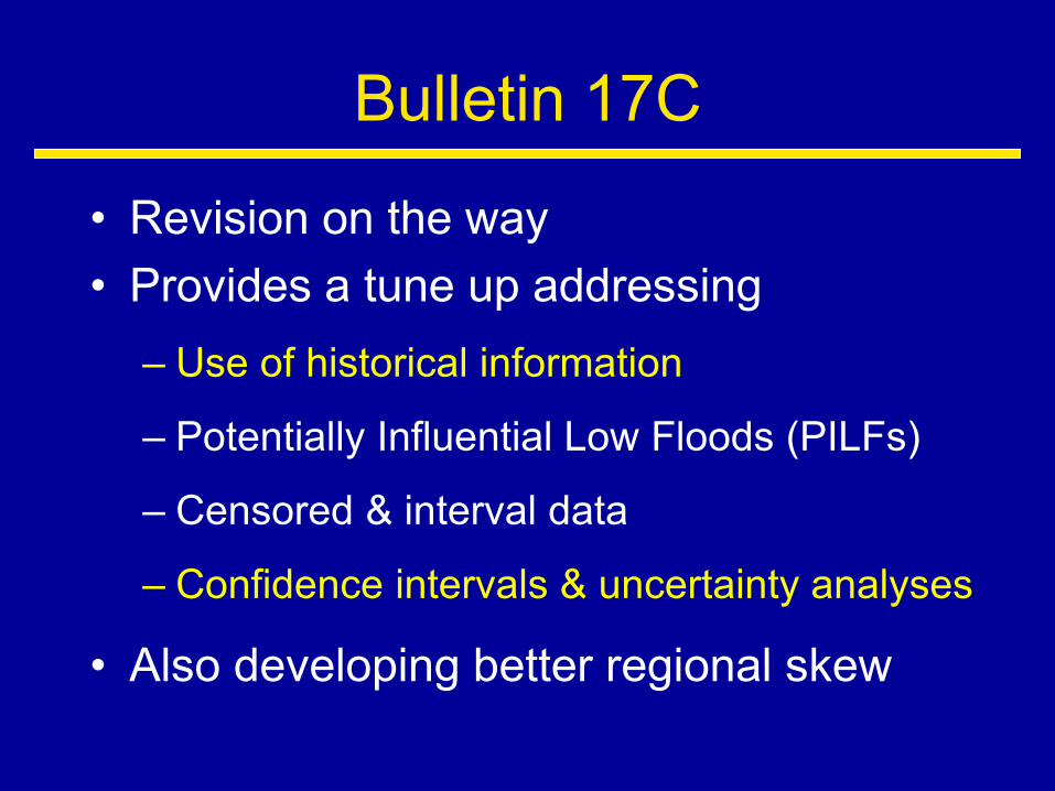
Bulletin 17C

• Revision on the way • Provides a tune up addressing

– Use of historical information

– Potentially Influential Low Floods (PILFs)

– Censored & interval data

– Confidence intervals & uncertainty analyses

• Also developing better regional skew

Regional Skew Estimation Regional skew Gg

from B17 skew map

-0.5 < Gg <+0.7

Map SE = 0.55

MSE[Gg] = 0.302

Effective record length = 17 yrs

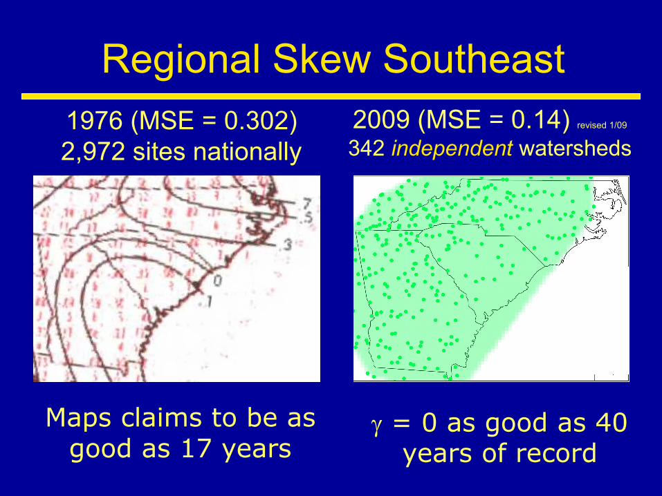
Regional Skew Southeast 1976 (MSE = 0.302) 2,972 sites nationally

2009 (MSE = 0.14) revised 1/09

342 independent watersheds

γ = 0 as good as 40 years of record

Maps claims to be as good as 17 years

Historial & Paleoflood data at a site:

Ways to extend the record.

Sources of Historical Information

Long-term Residences’ Memory Written accounts, markers, pictures

Geomorphologic evidence

slack-water deposits scour lines high-water marks undisturbed areas

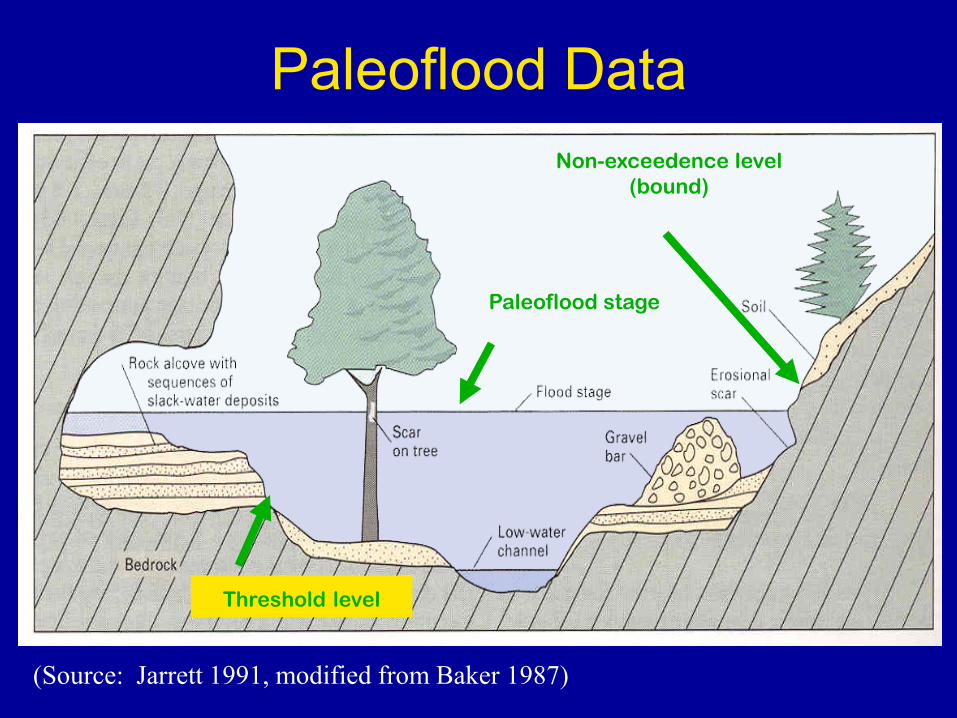
Paleoflood Data

(Source: Jarrett 1991, modified from Baker 1987)

Paleoflood stage

Non-exceedence level (bound)

Threshold level

Historical and Gauged Record

s years h years

Value of Historical Information

i.e. Bulletin 17B

S = 20

84

70

50 84 - 20 = 64 additional yrs 70 - 20 = 50 additional yrs 50 - 20 = 30 additional yrs

Value of Historical Information

S = 20

Value of Historical Information

i.e. Bulletin 17B

S = 20

40

24

40 - 20 = 20 additional yrs 24 - 20 = 4 additional yrs

Value of Historical Information

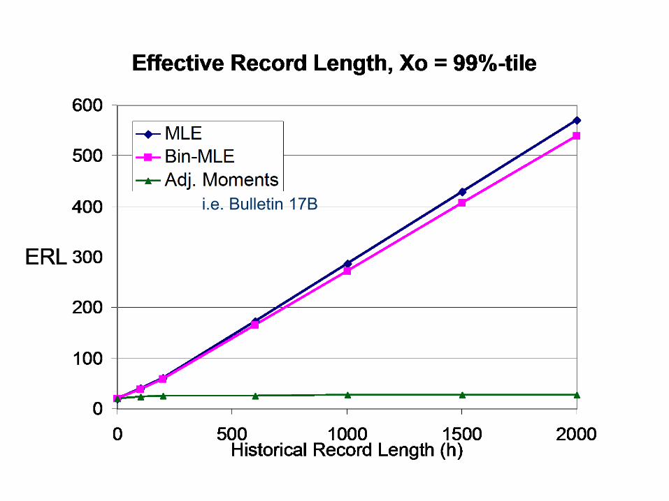
Effective record length

i.e. Bulletin 17B

Average Gains when Estimating 100-year Flood by fitting 2-Parameter Lognormal Distribution

(s = 20 years; h = 100 years)

i.e. Bulletin 17B

Average Gains when using MLE's to Estimate 1, 2, and 3 Lognormal Parameters

Observation:

Much larger Average Gains when estimating 3 parameters.

Shape parameter is hard to pin down with short records, and their estimators are sensitive to extreme observations.

Generalized Extreme Value (GEV) distribution

GEV Prob. Density Function large x

Index Flood & Regionalization

Substituting Space for Time.

Principles for better estimates of extreme flood probabilities

U.S. National Research Council report (1988) • Substitute space for time using "regionalization."

• Introduce additional structure into models based upon physical insight and hydrologic experience.

• Focus on extremes or "tails" of flood distribution, so less important and common floods do not distort fitted distribution for extreme events.

Hosking and Wallis (1997)

Development of L-moments for regional

flood frequency analysis.

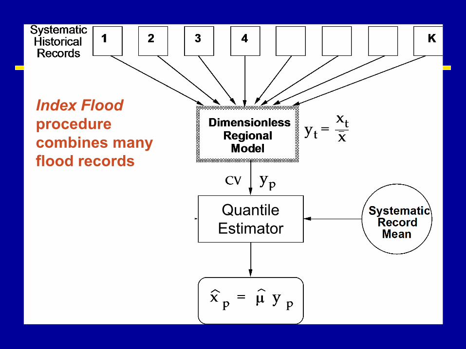
Index Flood procedure combines many flood records

Quantile Estimator

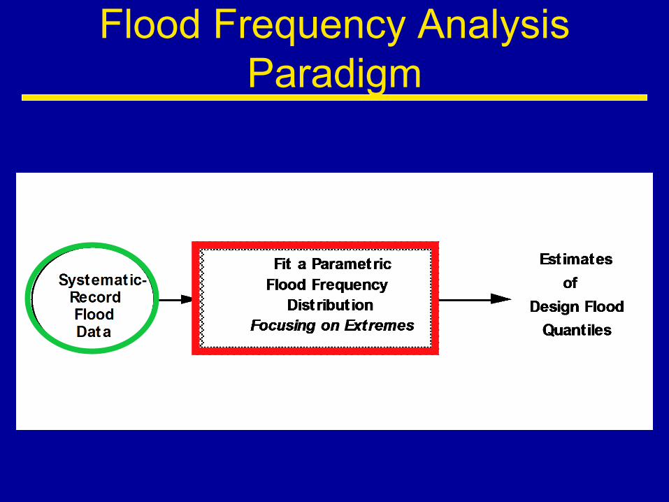
Flood Frequency Analysis Paradigm

New Paradigm for Flood Frequency Analysis

Credibility of Estimators

• At site record: 50 - 100 years • With historical info: 100-200 years • Regional 20 records: 20*50 = 1,000 years

• At-site & paleo. info: 1,000 years • At-site & regional paleofloods 10,000 years

See USBR(1999, 2004) for similar analysis of limits of credibility of empirical estimators

Empirical Analysis Assumes

• Observed records contains representatives of

critical events that represent LARGE & RARE floods at a site.

• Nature is “smooth” and “continuous” so that fitting a mathematically nice GEV or LP3 distribution is reasonable for extrapolation.

Estimating Flood Risk

B17B Empirical Use observed Flood Data

PFHA (?)

Imagine Construct using

regional flood, rainfall, climate,

storm-track, & orographic data

T = 100 to 1000 comfortably T = 10,000 to 1 million

Addressing Uncertainty

• Consider

Natural Variability (Aleatory Uncertainty) versus Knowledge Uncertainty (Epistemic Uncertainty-Limited data to estimate parameters)?

• Do they combined to get total risk?

• Do we give nominal risk with uncertainty bounds reflecting epistemic uncertainty?

• Flood risk estimates in US (following Bulletin 17B) include only aleatory uncertainty.

MCMC for LP3 Quantiles with only systematic information, s = 100

Ilustration of Uncertainty

Drew samples of size n = 100

From 2-parameter lognormal distribution.

Fit 2-parameter lognormal distribution AND

Fit 3-parameter LP3 (with log moments)

Estimated events exceeded with probability of

1 in 100 through 1 in a million.

Report ratio of exceedance probability of “design floods” to anticipated exceedance probability.

and Coefficient of Variation of “design flood” estimators.

Coefficient of Variation of Design Flood Estimators

1 in 100 1000 10,000 100k Million Nominal Exceedance Probability p

Consider 2-p Lognormal, and 3-p LP3 distributions

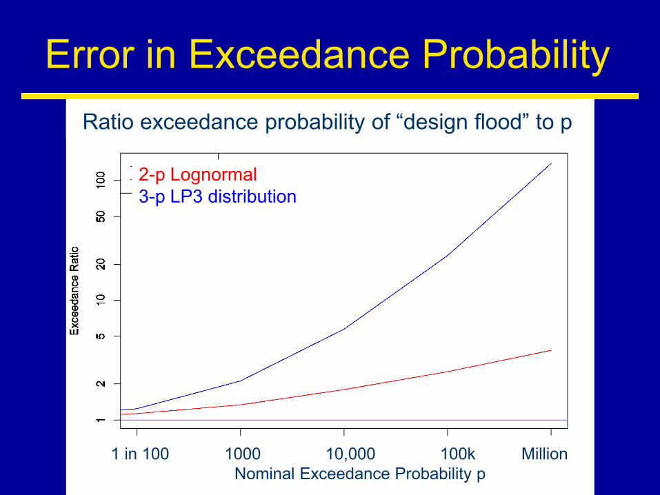
Error in Exceedance Probability Ratio exceedance probability of “design flood” to p

1 in 100 1000 10,000 100k Million Nominal Exceedance Probability p

2-p Lognormal 3-p LP3 distribution

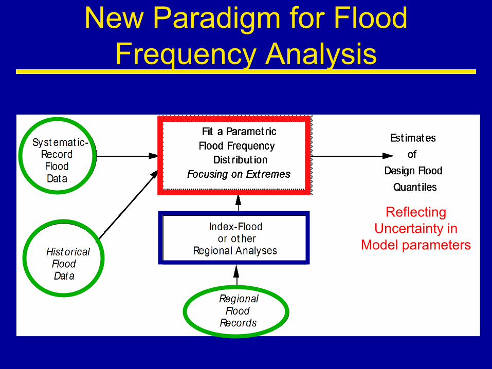
New Paradigm for Flood Frequency Analysis

Reflecting Uncertainty in

Model parameters

Historical advice

“We must accomplish a task more difficult to many minds

than daring to know. We must dare to be ignorant.”

Concluding two sentences: Karl Pearson

The Grammar of Science, 1892

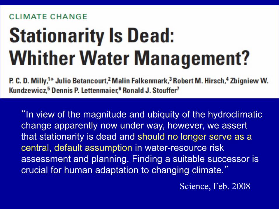
“In view of the magnitude and ubiquity of the hydroclimatic change apparently now under way, however, we assert that stationarity is dead and should no longer serve as a central, default assumption in water-resource risk assessment and planning. Finding a suitable successor is crucial for human adaptation to changing climate.”

Science, Feb. 2008

Clmate Change – So What?

(1) Gaged records tell us what common floods look like and where we start.

(2) Then we need to estimate the change.

(3) But how to determine where we go from here?

Climate Change & Risk Projection

• Imagine 50-100 year record of floods

• Plus paleoflood record illustrating largest floods over 1000-2000 years.

• Fit a line to estimate 1-in-100,000 risk ?

• Paleoflood record likely includes periods of greater & lesser risk, so risk extrapolation OVER estimates actual risk in our time frame.

Summary • Flood records for last century do not reveal reliably flood

risk of 1 in 10,000 or 1 in a million.

• At-site Historical and Paleoflood information helps.

• Regionalization of recent & paleoflood records helps

• Extrapolation more uncertain with 3-parameter LP3.

• Climate change confuses things

– Public loss of confidence in analysis

– Extrapolating beyond paleoflood data likely conservative

Issues for Discussion

• Records of real floods may be insufficient for our purposes: analysis instead needs to imagine.

• Uncertainty can be large part of computed total risk.

– Are we eady to combine variability & knowledge uncertainty into a total risk?

– Can we do the computation appropriately using honest informative Bayesian priors ?

Thank you for your attention.

Jery Stedinger

Donald Rumsfeld, Secretary of Defense under President George W. Bush from 2001 to 2006

said at Department of Defense news briefing, February 2002:

"Reports that say that something hasn't happened are always interesting to me, because as we know,

there are known knowns; there are things we know we know. We also know there are

known unknowns; that is to say we know there are some things we do not know.

But there are also unknown unknowns -- the ones we don't know we don't know.

And if one looks throughout the history of our country and other free countries, it is the latter category

that tend to be the difficult ones."

Generalized Extreme Value (GEV) distribution

Gumbel's Type I, II & III Extreme Value distr.:

F(x) = exp{ – [ 1 – (κ/α)(x-ξ)]1/κ } for κ ≠ 0

µX = ξ + (α/κ) [1 – Γ(1+κ)]

Var[ X ] = (α/κ)2 [Γ(1+2 κ) –- Γ2(1+κ)]

E[ (X-µX)3 ] = (α/κ)3 [ – Γ(1+3κ) + 3 Γ(1+κ) Γ(1+2 κ) – 2Γ3(1+κ) ]

κ = shape; α = scale, ξ = location. Mostly

-0.25 < κ ≤ 0