Extratropical Atmosphere-Ocean Variability in CCSM3

Michael Alexander1, Jeffrey Yin2, Grant Branstator2, Antonietta Capotondi1, Christophe Cassou3,

Richard Cullather4, Young-oh Kwon2, Joel Norris5, James Scott1, Ilana Wainer6

1 NOAA-CIRES Climate Diagnostics Center, Boulder, Colorado

2 National Center for Atmospheric Research, Boulder, Colorado

3 CERFACS-SUC, Climate Modelling and Global Change Team, Toulouse, France

4 Lamont-Doherty Earth Observatory, Columbia University, Palisades, NY

5 Scripps Institution of Oceanography, La Jolla, CA

6 Department of Physical Oceanography, University of São Paulo, São Paulo, Brazil

For JCLIM CCSM Special Issue

re-submitted June 2005

Corresponding Author:Michael AlexanderNOAA/CIRES, Climate Diagnostics CenterMail code: R/CDC1325 BroadwayBoulder, CO 80305Michael.Alexander@noaa.gov

1

Abstract

Extratropical atmosphere-ocean variability over the Northern Hemisphere of the Com-

munity Climate System Model version 3 (CCSM3) is examined and compared to observa-

tions. Results are presented for an extended control integration with horizontal resolution

of T85 (1.4°) for the atmosphere and land and ~1° for the ocean and sea-ice.

Several atmospheric phenomena are investigated including storms, clouds, and pat-

terns of variability and their relationship to both tropical and extratropical SST anomalies.

The mean storm track, the leading modes of storm track variability and the relationship of

the latter to tropical and midlatitude sea surface temperature (SST) anomalies are fairly

well simulated in CCSM3. The positive correlations between extratropical SST and low-

cloud anomalies in summer are reproduced by the model, but there are clear biases in the

relationship between clouds and the near surface meridional wind. The model accurately

represents the circulation anomalies associated with the jet stream waveguide, the Pacific

North American (PNA) pattern, and fluctuations associated with the Aleutian low, includ-

ing how the latter two features are influenced by El Niño/Southern Oscillation (ENSO).

CCSM3 has a reasonable depiction of the Pacific Decadal Oscillation (PDO), but it is not

strongly connected to tropical Pacific SSTs as found in nature. There are biases in the posi-

tion of the North Atlantic Oscillation (NAO) and other Atlantic regimes, as the mean Ice-

landic low in CCSM3 is stronger and displaced southeastward relative to observations.

Extratropical ocean processes in CCSM3, including upper ocean mixing, thermocline

variability and extratropical to tropical flow within the thermocline, also influence climate

variability. As in observations, the model includes the “reemergence mechanism” where

seasonal variability in mixed layer depth (MLD) allows SST anomalies to recur in consecu-

2

tive winters without persisting through the intervening summer. Remote wind stress curl

anomalies drive thermocline variability in the Kuroshio-Oyashio Extension region which

influences SST, surface heat flux anomalies and the local wind field. The interior ocean

pathways connecting the subtropics to the equator in both the Pacific and Atlantic are less

pronounced in CCSM3 than in nature or in ocean-only simulations forced by observed

atmospheric conditions, and the flow from the subtropical North Atlantic does not appear

to reach the equator through either the western boundary or interior pathways.

3

1. Introduction

Extratropical atmosphere-ocean processes exhibit variability on a broad range of time

scales, e.g. the intensity and path of storms change daily while ocean currents can fluctuate

over decades or more. These processes vary with the seasons, influence large-scale patterns

of climate variability and are linked to each other in complex ways. Many features of the

extratropical atmosphere and ocean system are influenced by local air-sea interaction and

remote teleconnections through their imprint on sea surface temperature (SST). The abil-

ity of climate models to simulate important aspects of the extratropical climate system,

including storm tracks, clouds, large-scale atmospheric circulation anomalies and upper

ocean mixing and circulation, is critical to our ability to understand and predict climate

variability and change. There are several benefits to using coupled general circulation

models (GCMs) to explore climate variability, including the archival of complete and

dynamically consistent fields, many of which are difficult to measure in nature, and the

ability to perform long simulations to isolate climate signals from noise. Here we explore

atmospheric and oceanic processes and their influence on Northern Hemisphere variabil-

ity on synoptic to decadal time scales in the Community Climate System Model version 3

(CCSM3).

Chang et al. (2002) noted the fundamental role of storm tracks in the climate system;

they generate much of the day to day weather variability in midlatitudes and are closely

linked to the planetary-scale flow. Changes in the position and strength of the storm tracks

can force the ocean via changes in the surface heat fluxes, which can exceed 1000 Wm-2 in

the vicinity of intense extratropical cyclones (Neiman and Shapiro 1993) and may respond

4

to the ocean via the influence of the SST gradient on the low-level atmospheric baroclinic-

ity (Nakamura et al. 2004).

While storm tracks are substantially weaker in summer than in winter, atmospheric

fluctuations can still have a substantial impact on SSTs, as the surface solar and latent heat

flux anomalies are large and the ocean mixed layer is shallow. Weare (1994) and Norris and

Leovy (1994) noted that total and low-level cloud anomalies are negatively correlated with

SST anomalies, which implies a positive feedback: increased cloud cover favors cooler SST

by reducing surface insolation, while cooler SST favors more stratiform cloud cover by

promoting a shallow and moist atmospheric boundary layer (Norris et al. 1998;

Frankignoul and Kestenare 2002; Park et al. 2004). The negative correlations are especially

pronounced between 25°N-40°N, where the mean meridional gradients in SST and cloud

amount are strong.

During both summer and winter atmospheric teleconnections from remote locations can

influence extratropical atmosphere-ocean variability. Principal among these is the

“atmospheric bridge”, where SST anomalies in the tropical Pacific associated with El Niño/

Southern Oscillation (ENSO) influence the North Pacific and other ocean basins via

changes in the atmospheric circulation (e.g. Alexander et al. 2002 and the references

therein; Alexander et al. 2004; Deser et al. 2005).

There are also sources of variability that are inherent to midlatitudes. Large-scale

patterns of atmospheric variability, such as the North Atlantic Oscillation (NAO), which

derive most of their energy from internal atmospheric processes, can drive changes in the

underlying ocean via surface heat and momentum fluxes (Cayan 1992; Iwasaka and

Wallace 1995). Another candidate for a midlatitude influence on the extratropical oceans

are the zonally oriented teleconnection patterns that are prominent during northern winter

5

(Branstator 2002). These patterns consist of chains of upper tropospheric highs and lows

centered along the planetary wave guide near the core of the subtropical jet. Since these

patterns extend throughout the depth of the troposphere, they have the potential to

influence the extratropical oceans.

The SST anomalies driven by changes in the storm tracks and large-scale atmospheric

circulation anomalies are spread throughout the surface layer of the ocean via turbulent

mixing. Namias and Born (1970, 1974) were the first to note a tendency for midlatitude

SST anomalies to recur from one winter to the next without persisting through the

intervening summer and hypothesized that the SST anomalies reappear due to the seasonal

cycle in ocean mixed layer depth (MLD). Temperature anomalies that form at the surface

spread over the deep mixed layer in winter and then remain at depth when it shoals in

spring. During summer, these thermal anomalies are sequestered within the seasonal

thermocline (approximately 25-120 m), while surface fluxes damp the temperature

anomalies within the mixed layer. When the MLD increases in autumn, the anomalies are

re-entrained into the surface layer, influencing the SST. This process, termed the

“reemergence mechanism” by Alexander and Deser (1995), occurs over a substantial

portion of the world’s extratropical oceans (Alexander et al. 1999; Watanabe and Kimoto

2000; de Cöetlogon and Frankignoul 2003).

Upper ocean processes, including the reemergence mechanism contribute to interan-

nual and decadal variability of the extratropical oceans. Pronounced decadal fluctuations

occurred over the North Pacific during the 20th century, which Mantua et al. (1997)

termed the Pacific Decadal Oscillation (PDO) based on transitions between relatively sta-

ble states of the dominant pattern of North Pacific SST anomalies. The spatial structure of

the PDO resembles a horseshoe with anomalies of one sign in the central Pacific and

6

anomalies of the opposite sign around the rim of the basin. The SST transitions were

accompanied by widespread changes in the atmosphere, ocean and marine ecosystems (e.g.

Miller et al. 1994; Trenberth and Hurrell 1994; Benson and Trites 2002). The myriad of

mechanisms proposed to explain decadal climate variability in the North Pacific, including

the PDO, can be classified into three broad categories: extratropical, tropically forced and

those due to tropical-extratropical interactions.

Extratropical mechanisms for SST variability include stochastic atmospheric fluctua-

tions that force the ocean through surface heat fluxes and by wind-driven adjustments in

the ocean circulation via Rossby waves (Frankignoul et al. 1997; Jin 1997; Zorita and

Frankignoul 1997). The latter may be especially important for decadal variability as the

westward propagating the long first baroclinic Rossby waves integrate wind stress forcing

(Sturges and Hong 1995; Frankignoul et al. 1997) and take approximately 5-8 years to cross

the North Pacific (Latif and Barnett 1994). Variability in the thermocline associated with

Rossby wave dynamics influences SSTs in the vicinity of the western boundary current and

its extension (Miller et al. 1998; Deser et al. 1999; Schneider and Miller 2001). If these SSTs

exert a strong positive feedback on the atmospheric circulation, air-sea interaction com-

bined with fluctuations in the extratropical ocean gyres may result in self-sustaining dec-

adal oscillations (Latif and Barnett 1994, 1996; Miller and Schneider 2000).

In tropically forced mechanisms for the PDO, atmospheric teleconnections from the

equatorial Pacific can impact North Pacific SSTs either through variability in the surface

fluxes at decadal time scales (Trenberth 1990, Graham et al. 1994, Deser et al. 2004) or by

ENSO-related forcing on interannual time scales which is subsequently integrated, or “red-

7

dened”, by the reemergence mechanism and wind forced Rossby waves in the North Pacific

(Newman et al. 2003; Schneider and Cornuelle 2005).

In the tropical-extratropical mechanisms for decadal variability, the atmospheric com-

ponent is essentially the same as in the tropical forcing paradigm, but the decadal time

scale is set by the ocean, either through the advection of ocean thermal anomalies from the

North Pacific to the equator (Gu and Philander 1997) or by changes in the strength of the

tropical-extratropical circulation (Kleeman et al. 1999; McPhaden and Zhang 2002). The

equatorward flow is part of a shallow (< 500 m) overturning circulation, termed the sub-

tropical cell (STC), where subtropical water subducts into the main thermocline, upwells at

the Equator, and then returns to the subtropics in the thin surface Ekman layer (e.g. Moli-

nari et al. 2003).

Here we examine extratropical atmospheric and oceanic processes and tropical-extrat-

ropical interactions in an extended CCSM3 control simulation and compare the results to

observations whenever possible. In general, we seek to understand mechanisms for the

evolution of Northern Hemisphere SST anomalies, as they play a crucial role in atmo-

sphere-ocean variability in the climate system. CCSM3 is briefly described in section 2;

storm tracks and their relation to SST anomalies are examined in section 3; the relationship

between clouds and atmosphere and ocean variability is examined in section 4; the domi-

nant patterns of atmospheric variability, including the PNA and NAO, are discussed in sec-

tion 5; the upper ocean thermal structure and reemergence mechanism are examined in

section 6; the dominant patterns of North Pacific SST and thermocline variability and their

relation to the tropical Pacific SST is investigated in section 7, and the extratropical-tropi-

8

cal flow within the thermocline is examined in section 8. The results are briefly summa-

rized in section 9.

2. Model description

The Community Climate System Model (CCSM), version 3, has four major

components representing the atmosphere, ocean, cryosphere and land surface. The

components are linked via a flux coupler, where no corrections are applied to the fluxes

between components. There have been improvements in several aspects of the model

relative to its previous version, CCSM2, including new treatments of cloud processes,

aerosol radiative forcing, land-atmosphere fluxes, ocean mixed-layer processes, and sea-ice

dynamics (Collins et al. 2005a).

The Community Atmosphere Model (CAM3, Collins et al. 2005b), is a global

atmospheric general circulation model (AGCM). The standard version of CAM3, which is

used here, has 26 vertical levels and is based upon the Eulerian spectral dynamical core

with triangular (T) truncation at 31, 42, and 85 wave numbers, horizontal resolutions of

approximately 3.75°, 2.8° and 1.4°, respectively. The Community Land Model (CLM,

Oleson et al. 2004) grid is identical to that of CAM3. The ocean general circulation model

is an extension of the Parallel Ocean Program (POP, Danabasoglu et al., 2005) originally

developed at Los Alamos National Laboratory. For resolutions of T42 and higher, POP has

40 vertical levels and a nominal horizontal resolution of 1°: uniform zonal resolution of

1.125° and meridonal resolution that varies from 0.27° near the equator to more than 0.5°

poleward of 30°. The Community Sea-Ice Model (CSIM, Briegleb et al. 2004) grid is

identical to POP’s.

9

Here we focus on an extended (> 600 year) control simulation of CCSM3 at T85

resolution for the atmosphere and land and the ~1° grid for ocean and sea-ice, the

configuration used in the NCAR climate-change simulations. In control integrations, the

CO2 is fixed at present day values. A similar control CCSM3 simulation was performed

using the T42 version of CAM3. The T42 and T85 control simulations are compared to

each other and to observations on the web (Stevens et al. 2005, http://www.cgd.ucar.edu/

cms/stevens/master.html, where the T42 and T85 control integrations are referenced as

experiments b30.004 and b30.009). The results from the T42 version are not presented here

as most variables we examined were similar to those in the T85 experiment, but notable

differences between the two experiments are discussed in the text. In section 8, an

uncoupled POP simulation forced with observed atmospheric conditions over the period

1958-2000 is also used to study the flow within the thermocline.

3. Storm tracks and their relation to SST anomalies

We assess the atmospheric variability associated with storm tracks in CCSM3 using

both a cyclone tracking algorithm and transient eddy statistics based on bandpass-filtered

data to retain variability on synoptic time scales (e.g., Blackmon et al. 1977). The two

provide complementary information: the former indicates the trajectories of both surface

lows and highs, while the latter emphasizes the magnitude of tropospheric variability in the

Pacific and Atlantic storm tracks. In the tracking algorithm, both the ERA40 and CCSM3

sea level pressure (SLP) fields are interpolated to a polar stereographic grid with ~200 km

resolution. A low (or high) pressure feature is identified if a given grid point is lower

(higher) than any surrounding points within 800 km. The exact location and value of the

feature is obtained using a descent method that employs bi-directional polynomial

10

interpolation (Powell, 1964). Cyclone tracks are constructed by performing a nearest

neighbor search within 1500 km at a location downstream from the low at the previous

time as predicted by the monthly-averaged 700 hPa wind field. Storm tracks are also

represented by 300 hPa geopotential height variance (z’2), which is calculated using daily

data that is high pass filtered to retain fluctuations on synoptic time scales (~2-8 days). The

observational data are from the European Center for Medium-Range Weather Forecasts

(ECMWF) 40-year Re-Analysis (ERA-40). ERA-40 2.5° lat x 2.5° lon 6-hourly sea level

pressure (SLP) and geopotential height fields have been averaged to produce daily mean

fields. The data are compared to daily output from the CCSM3 T85 simulation during

December-March (DJFM), where the years specified correspond to JFM of a given winter.

The average of the cyclone trajectories during boreal winter in ERA-40 (years 1958-

2000) and in CCSM3 (years 501-540) are very similar over the open oceans, but ERA-40

has more storm activity at both the beginning and end of the Pacific and Atlantic storm

tracks (Fig. 1). The model also underestimates the number of cyclones over the

Mediterranean and to the south of the Caspian Sea. In addition, ERA-40 indicates a local

maxima in the lee of the Rocky Mountains that is much weaker and more diffuse in the

model. This deficiency is slightly less marked in the T85 simulation than in the T42

simulation (not shown), suggesting that the resolution of topography may be a factor in

determining lee cyclogenesis in the model. The anticyclone tracks in CCSM3, which

extend over most of the North Pacific and from Hudson Bay (65°N, 80°W) to the Kara Sea

(75°N, 70°E), are strikingly similar to observations (not shown).

The influence of ENSO on storm tracks is depicted in Fig. 2, based on the composite

difference in storm track density between the ten winters with the warmest and coldest

11

SSTs in the Nino3.4 region (5°N-5°S, 170°W-120°W) during 1958-2000 in ERA-40 and

years 501-540 in CCSM3. In the eastern Pacific, there is a meridional dipole anomaly

between about 160°W-130°W, which indicates a southward displacement of the cyclone

trajectories in the storm track exit region during El Niño events in both ERA-40 and

CCSM3. The equatorward shift in the storm track over the central and eastern Pacific is

consistent with previous observational and modeling studies (e.g. Straus and Shukla 1997;

May and Bengston 1998; Compo et al. 2001), and a robust feature in CCSM3, as indicated

by regressions between SST anomalies in Nino3.4 and band pass filtered 300 hPa z’2 during

years 501-540 and in years 101-600 (not shown). Both the model and observations display

a significant decrease in storm activity to the south of the Kamchatka Peninsula in the

western Pacific, but unlike observations, CCSM3 indicates a significant enhancement in

storm activity over eastern Siberia. The model also overestimates the spatial extent of the

ENSO-induced change in the number of storms over the North American section of the

Arctic. In agreement with Compo et al. (2001), ERA-40 indicates a southward

displacement of the storm track along the eastern seaboard of the United States, a feature

that is present albeit weaker and less robust in CCSM3.

Empirical orthogonal function (EOF) analysis is used to calculate the leading modes of

interannual variability of the Pacific and Atlantic storm tracks during DJFM. Regressions

of 300 hPa z’2 on the principal components (PCs) of the two leading modes of 300 hPa z’2

variability for years 101-600 of the CCSM3 control run over the Pacific (120ºE-120ºW,

20ºN-80ºN) and Atlantic (90ºW-30ºE, 20ºN-80ºN) are shown in Fig. 3, superimposed on

the climatological storm tracks. Over both the Pacific and Atlantic, EOF 1 indicates a

12

meridional shift of the storm track exit, while EOF 2 indicates a strengthening of the storm

track.

The same EOF analysis is performed on the DJFM storm tracks in ERA-40 for the

period 1958-2000. While Harnik and Chang (2003) show that the NCEP-NCAR reanalysis

underestimates upper-level storm track strength relative to radiosonde observations prior

to the late 1970s, the storm tracks are stronger in ERA-40 than in NCEP-NCAR for the

period 1958-1978 (not shown); including the years before 1979 has little effect on the EOF

analysis aside from a reordering of the first 3 Atlantic EOFs. For both the Pacific and

Atlantic in ERA-40, EOF 1 is a strengthening of the storm track and EOF 2 is an equator-

ward shift of the storm track exit; regressions of 300 hPa z’2 on the corresponding PCs are

shown in Fig. 4. Differences between CCSM3 and ERA-40 modes of storm track variability

appear related to biases in CCSM3 climatological storm tracks, which are similar to those

found in CAM3 (Hurrell et al. 2005).

To investigate whether these modes of interannual storm track variability are coupled

to extratropical SST and land temperatures, surface temperatures in CCSM3 and ERA-40

are regressed on the corresponding storm track PCs (color shading in Figs. 5 and 6). All of

the modes of variability except for the strengthening of the Atlantic storm track in CCSM3

are accompanied by patterns of SST that have the potential to reinforce the storm track pat-

tern, i.e. an increase in the meridional SST gradient equatorward of where the storm track

increases in strength, as the storm track is most influenced by the surface temperature gra-

dient 5º to 10º equatorward of its latitude due to the poleward tilt of baroclinic waves with

height (Yin and Battisti 2004). While SST changes little with a strengthening of the Atlantic

13

storm track in CCSM3, the surface temperature gradient is enhanced upstream over North

America, as was found by Guylev et al. (2002).

Regressions of 1000 hPa zonal wind on the PCs of storm track variability (contours in

Figs. 5 and 6) show that low-level winds tend to be more westerly where SSTs are cooler

over the Pacific, implying that the SST anomalies are driven by winds either through sur-

face heat fluxes or Ekman transport across the meridional SST gradient. This relationship

also appears to hold in the Atlantic, although in CCSM3 the stronger zonal winds near the

east coast of the U.S. appear to be offset by another process, probably either advection by

anomalous southerly winds or increased ocean heat transport by a stronger wind-driven

subtropical gyre. In turn, the changes in low-level zonal winds are consistent with the

changes in poleward heat and momentum flux that are expected to accompany the shifts in

the storm tracks.

The relationship between the storm tracks and SST in June-August (JJA) is somewhat

less clear. The first EOF of JJA 2-8 day 300 hPa z’2 is a weakening and equatorward shift of

the storm track in both the Pacific and Atlantic in CCSM3 and ERA-40 (black contours in

Fig. 7), although the patterns are somewhat stronger and more extensive in the model. The

poleward shift of CCSM3 storm track EOFs relative to ERA-40 reflects the poleward shift

of the JJA mean storm tracks relative to ERA-40 (not shown), which is also found in CAM3

(Hurrell et al. 2005). The SST anomalies regressed on the corresponding storm track PCs

(color shading in Fig. 7) shift the strongest meridional SST gradient equatorward, and thus

may reinforce the storm track anomalies. Lag regression analysis shows that the SST anom-

alies are largest when they lag the storm track anomalies by about one month in both sum-

mer and winter (not shown), implying that the atmosphere is forcing the SST anomalies,

14

but the link between the storm track and the SST forcing is not clear in JJA. Although the

1000 hPa zonal wind anomalies regressed on the storm track PCs (not shown) line up rea-

sonably well with the SST anomalies in the Atlantic, in the Pacific the SST and zonal wind

anomalies are in approximate meridional quadrature and further analysis is required to

explain the forcing of the SST anomalies that accompany the dominant pattern of JJA

storm track variability over the North Pacific. However, it is encouraging that the relation-

ship between storm tracks and SST is similar between CCSM3 and observations in both

summer and winter. While there is a close correspondence between the storm track related

temperature anomalies in CCSM3 and ERA-40 over the ocean, differences between them

are more pronounced over the continents during summer and winter.

4. Summertime cloud-SST variability

Changes in clouds are associated with synoptic and lower frequency variability during

both summer and winter, but clouds mainly impact the extratropical oceans during

summer by altering the shortwave radiation reaching the surface. During summer,

meridional advection ahead of and behind cold fronts in extratropical cyclones strongly

influences low-level clouds via interaction with the underlying ocean (e.g. Norris et al.

1998). Poleward advection of warm subtropical air over colder water enhances

stratification leading to saturation of the boundary layer and the formation of fog or

shallow stratus (Norris 1998; Norris and Klein 2000; Norris and Iacobellis 2004), while

equatorward advection of midlatitude cold-sector stratocumulus over warmer water leads

to decoupling of the cloud and subcloud layers and subsequent stratocumulus breakup

(e.g., Wyant et al. 1997). As a result, the climatological low-to-mid level cloud fraction is

15

high (low) north (south) of ~40°N over the northern oceans during boreal summer, which

is simulated reasonably well in CCSM3 (see Stevens et al. 2005).

The correlation between low-level cloud amount and SST over the midlatitude North

Pacific and North Atlantic during JJA in observations and CCSM3 are shown in Fig. 8.

Individual ship low-level cloud cover reports collected in the Extended Edited Cloud

Report Archive (EECRA, Hahn and Warren 1999) and monthly SST anomalies from

Kaplan et al. (2000) were averaged over JJA and within 5ºx10º grid boxes during 1958-97.

Corresponding monthly CCSM3 low-level cloud fraction and SST values from twelve

sequential 40-year segments (years 100-579) were also averaged over JJA and linearly

interpolated to the observed grid. The availability of twelve realizations enables an

assessment of the likelihood that differences between CCSM3 and observed correlations

are not merely due to chance. CCSM3 reproduces the observed bands of large negative

cloud-SST correlation across the North Pacific and North Atlantic between 30ºΝ-50ºN as

well as areas of negative correlation over eastern subtropical oceans, near the southeastern

U.S., and near the British Isles (Fig. 8). These negative correlations indicate that low-level

clouds act as a positive feedback on SST anomalies in CCSM3, as occurs in nature (e.g.,

Norris et al. 1998; Frankignoul and Kestenare 2002; Park et al. 2004). However, the cloud-

SST correlations are more negative in CCSM3. Sampling uncertainty may be a contributing

factor to the weaker observed correlations, but there may also be an unrealistic sensitivity

between low-level cloud fraction and SST in CCSM3. The unrealistic negative correlation

exhibited by CCSM3 in the western subtropical North Pacific probably has little impact on

the simulation because the magnitude of interannual low-level cloud anomalies in this

region is very small (not shown).

16

Despite the general resemblance of observed and CCSM3 low-level cloud-SST

correlation patterns, not all cloud processes are correctly represented in the model. The

correlation between low-level cloud amount and near-surface meridional wind component

obtained from monthly values of National Centers for Environmental Prediction (NCEP)

reanalysis 1000 hPa wind (Kalnay et al. 1996) and CCSM3 lowest layer wind are shown in

Fig. 9. Although CCSM3 reproduces the observed negative correlation between low-level

cloud amount and meridional wind over eastern subtropical oceans, it exhibits positive

rather than negative correlations over the midlatitude North Pacific and North Atlantic.

The primary cause of the erroneous correlations in CCSM3 is that the large-scale cloud

fraction parameterization underproduces midlatitude stratocumulus when there is

southward flow, a problem common to other AGCMs (e.g., Tselioudis and Jakob 2002),

while overproducing stratus clouds around 40°N when warm air is advected over cold

water.

5. Atmospheric and SST Patterns of Variability

Much of the variability in the extratropical atmosphere and ocean occurs in coherent

large-scale patterns. In this section, we examine the patterns of variability in the Pacific

and Atlantic sectors and their relationship to local air-sea interaction and tropical forcing.

a. Waveguide patterns

Anomalies associated with the atmospheric waveguide, consisting of alternating highs

and lows near the core of the subtropical jet during winter, have been found in an earlier

investigation of two AGCMs and nature (Branstator 2002). They are of interest to our

study because they have the potential to initiate North Pacific large scale air-sea interaction

17

from remote midlatitude locations. Here we employ one-point correlation plots of monthly

anomaly fields to determine whether these patterns are also present in the CCSM3 control

integration and to see whether they interact with the extratropical North Pacific Ocean.

Prior to computing correlation patterns for a field, remote tropical influences are removed

using a linear regression relationship between interannual variations in grid point values of

that field and concurrent interannual variations in the first ten principal components of

Southern Hemisphere monthly mean 300 hPa stream function. This filter is based on the

notion that Northern Hemisphere variability associated with Southern Hemisphere

variability is instigated by tropical SST anomalies.1

To verify that the waveguide teleconnection patterns occur in CCSM3, we produced

one-point correlation plots of 300 hPa stream function for January means during years

100-599 of the CCSM3 T85 control integration. Fig. 10 shows the one point correlation

chart for a master point at 127.5°E, 33°N. This map is qualitatively similar to many such

charts with master points in the vicinity of the Asian subtropical jet and shows that CCSM3

does have zonally oriented patterns that extend across the expanse of the Northern

Hemisphere like those found by Branstator (2002). Consistent with the linear model

solution of Rossby wave propagation (Branstator 2002), the phase of this pattern shifts

longitudinally if one moves the longitude of the master point and its zonal extent is also

affected by such shifts. For example, with a master point at 90°E, 29°N the atmospheric

anomalies are confined to the western half of the North Pacific (not shown) rather than the

circumpolar pattern seen in Fig. 10.

1. A more conventional filter based on the leading principal components of tropical SSTvariability gave qualitatively similar results, though it appeared to remove midlatitudeinitiated relationships with the tropics, an undesirable characteristic for our study.

18

Having established that waveguide patterns exist in CCSM3, we seek to determine

whether they interact with the underlying ocean. One indication that there is such an

interaction comes from calculating correlations between 300 hPa January stream function

at the master point used in Fig. 10 and simultaneous variations in SLP (Fig. 11a) and

surface temperature (Fig. 11b). These correlations indicate that the upper tropospheric

circumglobal pattern is strongly connected to surface atmospheric and oceanic variations,

with the linkages being especially strong over the North Pacific. In particular, SLP

anomalies are nearly collocated with height anomalies at 30°N, 125°E and 35°N, 170°W,

while the associated surface temperature anomalies are located where the SLP gradient and

thus the winds and temperature advection are strong. (All of the features discussed here

occur in both the first and second half of the GCM record and thus appear to be robust.)

To investigate whether this association between the waveguide pattern and SST

anomalies is initiated in the atmosphere or ocean, we calculate the correlations between

the waveguide pattern and thermal fluxes (sensible heat, latent heat, net longwave

radiation and net shortwave radiation). There are substantial correlations in some regions

of the North Pacific for all of these quantities, but regression analyses indicate that the

magnitude of the radiation flux anomalies are weak compared to the heat fluxes (not

shown). The latent and sensible heat flux correlations (Fig. 11c-d) indicate that where SST

is above normal there is above average atmosphere-to-ocean heat flux, and where the SST

is below normal there is below normal atmosphere-to-ocean heat flux. Thus, the fluxes are

generally consistent with the atmosphere driving the ocean throughout the North Pacific.

The properties we have noted for the waveguide pattern in Fig. 11 are true for all other

patterns associated with the subtropical jet that we have examined; they all influence the

North Pacific through heat fluxes, though the geographical reach of the fluxes depends on

19

the longitudinal phase of the circulation anomalies.

Since in CCSM3 the interaction of the circumglobal waveguide pattern with the ocean

is one of the atmosphere forcing the ocean, given the ocean’s large thermal inertia one

would expect to find larger correlations of this atmospheric pattern with lagged rather than

simultaneous SST. Fig. 12a shows February surface temperature correlated with January

300 hPa streamfunction at 127.5°E, 33°N. All of the main midlatitude North Pacific

features are indeed stronger than they were for simultaneous correlations (Fig. 11b). One

month lagged correlation plots of other quantities including 300 hPa streamfunction and

surface heat fluxes (not shown) indicate that the atmospheric processes that produced the

North Pacific SST anomalies in January have almost disappeared by February. Thus it is

not surprising that two month lagged surface temperature correlations (Fig. 12b) are

weaker than their one month lagged counterparts since the atmospheric anomalies are no

longer there to help maintain them.

Spurred by studies like that of Barsugli and Battisti (1998), a commonly asked question

is whether the atmospheric-induced midlatitude SST anomalies feed back onto midlatitude

atmospheric anomalies, and if so whether the feedback is positive. For the waveguide

initiated North Pacific anomalies, we do see a positive feedback in the sense that lagged

midlatitude temperatures in the lowest atmospheric level have substantial persistence with

a structure that matches underlying lagged SST anomalies (not shown). Since the upper

tropospheric waveguide patterns in the lagged months are nearly gone, these near surface

temperatures are almost certainly being supported by the ocean anomalies. However, the

negligible amplitudes of the lagged upper tropospheric anomalies indicate that the

feedback does not reach these levels in any substantial way.

20

b. North Pacific variability

The low-frequency extratropical atmospheric circulation is generally described in

terms of “teleconnection patterns” (e.g. Wallace and Gutzler 1981), which are spatially

stationary structures whose amplitudes fluctuate in time. Typically these patterns are

identified using techniques that assume linear behavior so that events in which the pattern

has one sign are just as important as events of the opposite sign in representing observed

behavior. Atmospheric variability can also be examined through a non-linear analysis

known as cluster decomposition (Andelberg 1973). This method, based on classification

techniques, seeks preferred and/or recurrent quasi-stationary atmospheric patterns or

“regimes” that are spatially well defined (but without symmetry constraints) and limited in

number. While regime analyses can provide useful information on the pattern and polarity

of climate anomalies, their significance in identifying non-normal behavior is uncertain

due to the limited number of observations (e.g. Stephenson et al. 2004). Thus, consistency

between regimes identified in observations and long climate model simulations can

provide additional evidence of their validity.

Climate regimes over the North Pacific (130oE-80oW, 20oN-80oN) are first

determined in individual winter months (December-March) during years 100-599 of the

CCSM3 control simulation. We used the k-mean partitional scheme (Michelangeli et al.

1995) and found k=4 to be the optimal number of statistically significant regimes to be

retained. The SLP field in each winter month is classified into one of the four regimes.

Composite maps of SLP anomalies for the sets of months belonging to each regime are

shown in Fig. 13a-d. The first two regimes are the Pacific North American (PNA+) pattern

and its opposite (PNA-) (Wallace and Gutzler 1981). Spatial asymmetries between the two

phases are found in the eastward extension of the North Pacific anomalous pressure

21

centers and in the related southward penetration of the higher latitude core over the North

American continent. Regimes 3 and 4 form another pair with an anomaly center near

Alaska. The strong high in the former is often associated with blocking conditions, while

the deepening and eastward shift of the Aleutian Low in the latter could be viewed as the

regional signature of the “Tropical North Hemisphere” (TNH) mode (Barnston and

Livezey 1987; Straus and Shukla 2002). Regime 3 and 4 will be henceforth referred to as

ALE+ and ALE- respectively. Counterparts can be found in observations as identified by

Robertson and Ghil (1999) or Michelangeli et al. (1995), although decompositions were

conducted from low-pass filtered daily maps instead of monthly means. PNA+ and PNA-

are equally excited (26% occurrences) and represent about half of the total sample, while

ALE- occurs more often (29%) than ALE+ (19%) in the model.

It is well known that the North Pacific extratropical atmosphere is affected by

anomalous SST conditions in the entire Pacific basin. Composite DJFM average surface

temperature (TS) anomalies are constructed when at least three of four months are

occupied by a given regime (see Cassou et al. 2004 for further details). All regimes are

associated with SST anomalies in both the tropical and North Pacific that are the hallmark

of ENSO (Fig. 13e-h). PNA+ (PNA-) is linked to the warm (cold) phase of ENSO and to

North Pacific SST anomalies associated with the atmospheric bridge mode characterized

by warm (cold) oceanic conditions along the North American west coast and colder

(warmer) SSTs in the central basin. Anomalous TS over the continents show contrasts

between the sub-polar areas of North America and Eurasia. Both ALE regimes are linked

to ENSO: El Niño episodes are associated with a deepening of the Aleutian Low (ALE-),

while blocking episodes occur more often during La Niña.

22

To better illustrate the forcing role of ENSO, relative changes of occurrence for each

regime during El Niño and La Niña events are presented in Table 1. El Niño events clearly

favor the ALE- regime while strongly reducing the occurrence of the PNA- regime. The

ALE+ (ALE-) regime is less frequent during warm (cold) events. La Niña changes the

frequency of both PNA phases about equally, with a strong increase in the PNA- and

decrease in the PNA+ regimes. Together Fig. 13 and Table 1 suggest that the extratopical

response to ENSO in CCSM3 is asymmetric: cold events strongly impact the PNA pattern,

while warm events have less of an influence on the PNA pattern but a stronger influence on

the ALE regime. This asymmetry results in an eastward shift of the Aleutian low during

warm events compared to cold events, as found in some observational and modeling

studies (Hoerling et al. 1997; Hoerling et al. 2001). Other studies have found that the

observed nonlinearity in the PNA region may result from insufficient sampling and that

the asymmetric response to tropical SST or heating anomalies over the PNA region is

modest (Sardeshmukh et al. 2000; DeWeaver and Nigam 2002; Lin and Derome 2004). The

long record available from the CCSM3 control integration suggests that nonlinearities in

the PNA response to ENSO are possible, although it is unclear whether they are due to

asymmetries in the equatorial SSTs, tropical heating and/or the extratropical atmospheric

response to the tropical forcing.

Relative changes in the frequency of occurrence of the North Pacific atmospheric

regimes (Fig. 13) associated with PDO are significant but much weaker than for ENSO

(Table 1). The positive phase of the PDO, with cold water in the central North Pacific, is

associated with the positive (negative) phase of the PNA (ALE) pattern, while only the

PNA- regime is enhanced during the negative phase of the PDO.

23

c. North Atlantic variability

The four SLP regimes over the North Atlantic (20oN-80oN, 80oW-30oE), shown in Fig.

14a-d, are obtained following the same cluster analysis approach as used in the Pacific.

Regimes 1 and 2 depict the positive and negative phase of the NAO. The third cluster

displays a strong anticyclonic ridge off western Europe (ATL+) while the fourth is

dominated by a trough covering the entire northern portion of the domain (ATL-). With

the exception of regime 4, all have counterparts in nature, although there are differences in

the structure of the regimes relative to observations (Cassou et al. 2004). For example, the

model is able to simulate the eastward shift of the Azores High for NAO+ towards Europe,

as part of NAO variability, but the Icelandic low extends too far to the east, leading to

stronger than observed zonal flows. The high in the ATL+ pattern is displaced to the

northeast and does not include the wave pattern from the subtropics to the Baltic Sea as

found in observations. The latter is likely related to biases in the mean climate: the

Icelandic low is stronger and displaced to the southeast in CCSM3 relative to observations.

The NAO and ATL- regimes are very similar in CCSM3 and CAM3 (not shown), which

suggests that the biases in the North Atlantic regimes are mainly due to atmospheric

processes and not air-sea coupling.

As in nature, surface temperature anomalies associated with the NAO regimes have a

quadripole pattern over the continents adjacent to the North Atlantic Ocean, with

anomalies of opposite sign over the northern and southern portions of North America and

over northern Europe and North Africa (Figs. 14e-h). Over the ocean, SST anomalies bear

some resemblance to the North Atlantic tripole, especially for NAO-. The ATL+ (ATL-) is

associated with downstream warm (cold) SST anomalies that are consistent with the

atmosphere forcing the land or ocean. The ATL+ and ATL- regimes are weakly linked to El

24

Niño and La Niña events, respectively, in CCSM3 contrary to the connection found in

observations (c.f. Cassou et al. 2004). This bias is not found in CAM3 simulations (not

shown) and may be due to the overly strong connection between the North Pacific and

Atlantic Oceans via the atmosphere as discussed below.

The temperature patterns associated with both the NAO and PNA regimes extend

across the entire Northern Hemipshere and these patterns resemble each other, i.e. the TS

patterns for PNA+/NAO- and PNA-/NAO+ are similar. This suggests a connection

between the leading basin modes simulated in the model and the hemispheric Northern

Annular Mode (NAM, or Arctic Oscillation, e.g. Thompson and Wallace 1998). Indeed

NAM, with zonally symmetric SLP anomalies of opposing signs centered near the pole and

~45oN is the dominant pattern over the Northern Hemisphere in CCSM3 (not shown) as

in nature. However, the connection between the Pacific and Atlantic variability via NAM

appears to be overestimated in the CCSM3 compared to observations (not shown), a com-

mon model bias (e.g. Cassou and Terray 2001).

6. Upper Ocean Temperature and Mixed Layer Depth

The results from sections 3-5 suggest that extratropical atmospheric variability,

whether generated by internal dynamics or in response to tropical SST anomalies can force

extratropical SST variability. These midlatitude SST anomalies penetrate into the ocean

through physical ocean processes, such as vertical mixing and advection, and return to the

surface at another time and/or location. Furthermore, ocean processes not only modulate

thermal anomalies but can generate extratropical SST anomalies, via adjustments in the

thermocline. In the subsequent sections we explore the role of large-scale atmospheric

25

forcing, vertical mixing, thermocline adjustment and advection on the upper ocean and

climate of CCSM3.

The evolution of the ocean anomalies, whether forced by the atmosphere or generated

by ocean dynamics, are strongly influenced by the climatology of the upper ocean, includ-

ing the vertical structure of temperature, salinity, currents and MLD, which vary with sea-

son and location. The mean seasonal cycle of temperature and MLD from observations

and CCSM3 are presented in Fig. 15 for regions in the central North Pacific (35°N-45°N,

165°E-175°W) and North Atlantic (50°N-60°N, 20°W-40°W). The observed temperature

and MLD values are obtained from the World Ocean Atlas (Levitus et al. 1998) and

Monterey and Levitus (1997), respectively. Both the observed and simulated MLD values

are based on density criteria, but the former is the depth at which the density is 0.0125 kg

m-3 less than the surface density, while the latter, as defined by Large et al. (1997), is the

depth of the maximum vertical gradient that is nearest the surface. The model reproduces

the general structure of the seasonal cycle with maximum (minimum) temperatures at the

surface in September (March) and a strong seasonal thermocline, in which the temperature

decreases rapidly with depth beneath the mixed layer during summer. The temperatures

throughout the upper ocean are too cold (also see Large and Danabasoglu 2005), while the

wintertime MLD is underestimated, particularly in the Atlantic. A broader comparison of

MLD between the model and observations over the Northern Hemisphere Oceans indi-

cates that the pattern of the winter MLDs is well simulated but their magnitude is over

(under) estimated over much of the North Pacific (Atlantic); the summer MLDs are well

simulated in both basins (not shown).

26

The central North Pacific and Atlantic are candidate regions for the reemergence

mechanism as they undergo a large seasonal cycle in MLD, are remote from regions of sub-

duction and strong eddy activity, and are similar to areas where observations indicate that

SST anomalies recur from one winter to the next (Alexander et al. 1999; Timlin et al. 2002).

Regressions of CCSM3 temperature anomalies as a function of month and depth on tem-

perature anomalies averaged over the three upper model layers (0-30 m) during February-

-April (FMA) are shown for these two regions in Fig. 16. The regressions are computed at

each model point and then averaged over the respective regions. In the Pacific, the anoma-

lies extend over the depth of the mixed layer (120-140 m) in winter, and decrease only

slightly in amplitude between 50-100 m through September but are reduced by more than

50% in the surface layer over the same period. A portion of the signal, indicated by regres-

sion values of > 0.5°C, returns to the surface in the subsequent December-March. In the

North Atlantic, where the wintertime MLD exceeds 300 m (Fig. 15), the reemergence sig-

nal extends over greater depths and the values returning to the surface in the winter are rel-

atively high (>0.8°C) compared with the Pacific. The difference between the reemergence

mechanism in the two basins is consistent with the findings of Deser et al. (2003), which

showed that the deeper the winter MLD, the further the anomalies penetrate into the

ocean, which increases the effective thermal inertia of the system and enhances the winter-

to-winter persistence of SST anomalies.

A cross-basin view of the reemergence process is obtained by correlating temperature

anomalies in the summer seasonal thermocline, 65-85 m depth in August-September, with

SST anomalies from the previous January through the following April at each model grid

point. The correlation coefficients (r) at each model longitude are then averaged between

27

42°N and 52°N and displayed across the Pacific and Atlantic Oceans in Fig. 17. Evidence

for the reemergence mechanism is clearly seen across much of the North Pacific: relatively

high r values in the previous and following winter and low values in the intervening sum-

mer. In the Atlantic, the correlations suggest that reemergence occurs between 0°-20°W

and 30°W-50°W. The absence of recurring SST anomalies between 50°E and the North

American coast in CCSM3 is consistent with the observational analyses of Timlin et al.

(2002), who showed that the reemergence process did not occur in this region since the

summer-to-winter difference in MLD was less than 50 m.

7. Patterns of North Pacific Ocean Variability

a. The PDO and its relation to tropical SSTs

Extratropical SST and other surface ocean variables tend to have spatial and temporal

scales commensurate with the large-scale atmospheric forcing that predominantly drives

them. The dominant pattern of SST variability in the North Pacific, the PDO, is defined

using the leading EOF of monthly SST anomalies north of 20°N. The wintertime (Novem-

ber-March) average of the PDO index, the PC associated with EOF 1, is shown for a 100-

year period from both observations and the model in Fig. 18a-b. The observed values are

based on historically reconstructed SSTs for the period 1900-1999 (Mantua et al. 1997); the

model results are from years 500-599 in the CCSM3 control integration. While a direct

correspondence is not expected between the model and nature, both show pronounced

decadal variability, with periods of 10 years or more where the PDO index is predomi-

nantly of one sign.

28

We explore the spatial structure of the PDO by correlating it with the concurrent near

surface air temperatures during winter (Fig. 18c-d). Over the North Pacific, the simulated

and observed PDO temperature patterns are very similar, as both have negative

correlations between about 35°N-50°N in the central to western Pacific and positive

correlations along the coast of North America that extend southwestward toward Hawaii.2

The correlations in both the model and observations also suggest a downstream wave train

with centers of opposite sign over Alaska/western Canada and the southeast United States

(also see Stevens et al. 2005). However, CCSM3 is markedly different from nature in terms

of the PDO’s connection to the tropics: strong positive correlations across most of the

tropical Pacific in observations are absent in the model.

b. Thermocline variability and its relation to SSTs and air-sea interaction

In contrast to SST anomalies, thermocline variations are insulated from direct contact

with the atmosphere and are thus primarily driven by ocean dynamics. We examine the

evolution of the depth of the 26.8 σθ (=1026.8 kg/m3) isopycnal to study the thermocline

variability and its relation to the surface variables in the North Pacific during years 350-599

in the CCSM3 experiment. In the Pacific, the 26.8 σθ isopycnal is generally located at the

bottom of the main thermocline in both the CCSM3 simulation and observations (Roden

1998). The first EOF of the annual mean depth of 26.8 σθ north of 20°N in the Pacific has

anomalies of one sign between approximately 30°N-50°N with maximum amplitude in the

2. A similar spatial structure for the PDO in both observations and the model is obtainedfrom EOF 1 of the North Pacific SST anomalies, but the model has excessive amplitudeto the east of Japan, which is likely due to the greater than observed variance in thatregion.

29

Kuroshio-Oyashio Extension region centered along 40°N in the western Pacific (Fig. 19a).

Fluctuations associated with a one standard deviation change in the corresponding time

series reach a maximum of ~50 m in the vicinity of 40°N, 150°E. The Kuroshio-Oyashio

Extension is where the maximum meridional gradient in the climatological mean depth of

the 26.8 σθ surface is found, and thus, EOF 1 is likely associated with a north-south shift of

the axis of the Kuroshio-Oyashio extension. The PC associated with EOF 1 has a spectral

peak at around ~9 years, which is significantly different from a red noise spectrum at the

99% confidence level (Fig. 19c). Lag regression of the 26.8 σθ isopycnal depth onto PC 1

(not shown) indicates that this pattern originates from the eastern subpolar region around

45°N, 160°W, and slowly expands westward over the five years prior to when EOF 1 was

computed. This eastern subpolar region coincides with the location of the maximum in the

first EOF pattern of the wind stress curl. The decadal time scale is also consistent with

previous studies on the gyre-scale circulation changes in the North Pacific (Miller et al.

1998; Deser et al. 1999). EOF 2 has a wave-like pattern around the subpolar gyre north of

40°N (Fig. 19b). The associated PC has a spectral peak at around ~16 years that is

significant at the 99% confidence level (Fig. 19c). In the CCSM2 control experiment, the

predecessor of this simulation, a pattern very similar to EOF 2 in both time scale and

spatial structure clearly demonstrated counter-clockwise propagation around the subpolar

gyre. However, propagation associated with the EOF 2 pattern was not readily apparent in

CCSM3.

To what extent are the leading patterns of thermocline and Pacific SST variability

related? EOFs of DJFM SST anomalies between 20°S and 60°N in the Pacific indicate that

ENSO and a North Pacific mode are the first and second leading patterns of variability

30

(Fig. 20), consistent with the observational analysis of Deser and Blackmon (1995). EOF 1

has maximum loading in the central and eastern tropical Pacific and a secondary

maximum in the central North Pacific. The corresponding PC also has a strong spectral

peak at around the ENSO period and a secondary peak at ~20 years (not shown). EOF 2

has very little expression in the tropics. PC 2 of SST and PC 1 of the depth of the 26.8 σθ

surface are correlated (r=0.39, significant at 99% level), when the latter leads by 2 years.

In the Kuroshio-Oyashio extension region (35°N-45°N, 140°E-180°), the SSTs are

related to the surface heat flux and wind stress curl as well as the thermocline depth (Fig.

21). The local correlation between SST and thermocline depth anomalies is 0.69, while the

correlation between the SST and the upward net surface heat flux (wind stress curl)

anomaly in DJFM is 0.56 (0.34), when the SST anomaly leads by one year. These values are

all significant at the 99% level and increase to 0.71, 0.72, and 0.44, respectively, when the

time series are low-pass filtered for periods longer than 5 years. Therefore, in the Kuroshio-

Oyashio Extension region, a deeper than normal thermocline causes a warm SST anomaly,

which is damped by surface heat flux anomalies out of the ocean and induces a local

atmospheric response including cyclonic wind stress curl.

The leading EOFs of North Atlantic SSTs in CCSM3 during winter are less realistic

than in the Pacific (not shown). For example, the first EOF of SST between 20°N-60°N has

a meridional dipole pattern, as found in nature, but the amplitude of both anomaly centers

is overly concentrated near the nodal line at ~45°N (not shown). A similar bias was found

in an OGCM driven by observed atmospheric conditions, but not in mixed layer ocean

model simulations driven by the same forcing (Seager et al. 2000), indicating that

inaccurate representation of ocean dynamics may be responsible for these errors. The

31

errors in variability are likely tied to those in the mean ocean circulation, as the Gulf

Stream is too zonal and the subpolar gyre too extensive in CCSM3 and in a ocean only

simulation forced by observed atmospheric conditions (Large and Danabasoglu 2005).

8. Extratropical-Tropical Ocean Pathways

Variations in the extratropical oceans may induce decadal changes in the tropics either

by the mean equatorward advection of subducted temperature anomalies (Gu and Philan-

der 1997) or by anomalous advection across the mean temperature gradients (Kleeman et

al. 1999). Both mechanisms require that the climatological ocean pathways within the sub-

tropical cell (STC) be simulated reasonably well. In the Pacific, observations indicate that

the presence of the Intertropical Convergence Zone (ITCZ) in the northern Tropics (7°-

10°N) creates a “potential vorticity (PV) barrier” for the equatorward flow, which is absent

in the Southern Hemisphere (Johnson and McPhaden 1999; McPhaden and Zhang 2002).

As a result, the interior (i.e. away from the western boundary) flow from the northern sub-

tropics follows a much more complex route than the equatorward flow from the Southern

Hemisphere. Thus, the Southern Hemisphere may play a greater role in tropical decadal

variability than the Northern Hemisphere (Change et al. 2001; Luo and Yamagata 2001).

The ocean component of CCSM3, driven by observed surface forcing over the period

1958-2000 (hereafter POP simulation) yields a PV field (Fig. 22a) that is very similar to

that computed from observations (c.f. Fig. 2c of Johnson and McPhaden 1999, and Fig. 1b

of McPhaden and Zhang 2002), although the PV ridge in the 7°N-10°N band is somewhat

weaker in the POP simulation. Fig. 22a shows the PV on the 25σθ isopycnal, a density sur-

face that lies within the core of the equatorial thermocline. In the Northern Hemisphere,

32

the flow is mainly zonal in the 7°N-10°N band, and feeds the western boundary current,

while equatorward flow is confined west of ~140°E.

The potential vorticity field on the 25σθ isopycnal in the Pacific from the CCSM3 sim-

ulation is shown in Fig. 22b. The PV barrier in the Northern Hemisphere is somewhat

stronger than in the POP simulation, and extends further west. The main difference

between PV in CCSM3 and POP (as well as observations) is a second area of large PV val-

ues in the western tropical South Pacific (150°E-180°), associated with the erroneous pre-

cipitation maximum located across the Pacific at ~8°S in CCSM3 (Deser et al. 2005; Hack

et al. 2005; Large and Danabasoglu 2005) and most other coupled GCMs (e.g. Covey 2003).

This southern PV barrier alters the flow pattern with respect to the POP simulation.

Around 10°S, the isopycnal flow in CCSM3 is more zonal, flowing westward and then

northward around the western side of the PV maximum. Thus, pathways connecting the

subtropical Pacific to the equator exist in CCSM3, but in the Southern Hemisphere they

are not as direct as found in observations and in the POP simulation.

In the Atlantic Ocean most of the water reaching the equator via the STC originates in

the Southern Hemisphere, although interior and western boundary pathways are found in

both hemispheres (e.g. Hazeleger et al. 2003; Zhang et al. 2003; Molinari et al. 2003).

Lagrangian trajectories are computed on the 25.4σθ isopycnal surface, which is located

within the tropical thermocline and intersects the equator near the core of the equatorial

undercurrent. Trajectories of “floats” released where the 25.4σθ outcrops are shown at one

year intervals in Fig. 23 for the POP and CCSM3 simulations; a similar observationally-

based analysis is presented by Zhang et al. (2003, Fig. 5). Like observations, the broad

structure of the flow in POP and CCSM3 is cyclonic on either side of the equator:

33

clockwise (counterclockwise) in the Southern (Northern) Hemisphere. However, there are

notable differences in the structure and in some locations the speed of the flow. In CCSM3,

only water from the Southern Hemisphere reaches the equator, predominantly through the

western boundary current, while in the POP simulation and observations there are also

pathways to the equator from the Northern Hemisphere and within the interior of the

South Atlantic Ocean. Trajectories on the 24.5σθ and 26.0σθ isopycnal surfaces (not

shown) suggest that the northern pathway to the equator is absent throughout the

thermocline in CCSM3. As in the Pacific, the biases in the circulation are consistent with

excessive PV maxima that extend across the subtropics of both hemispheres (not shown).

The current speed, as indicated by the distance between triangles, is similar in the two

integrations, except to the west of ~20°W in the Southern Hemisphere, where the flow

appears to be faster in CCSM3.

The CCSM3 simulation also contains a clockwise circulation in the southeast portion

of the basin that is not found in the POP simulation. While observations suggest that a

domed cyclonic circulation, termed the Angola gyre, exists in this location, the density

level and strength of the circulation are inaccurate in CCSM3 due to biases in the coupled

atmosphere-ocean system off the coast of southern Africa (see Large and Danabasoglu

2005).

9. Discussion and Conclusions

In this study, we have explored processes that influence extratropical climate variability

in CCSM3 with a focus on coupled atmosphere-ocean interaction. In both nature and

CCSM3, atmospheric processes, including storm tracks, clouds and climate regimes, influ-

34

ence large-scale atmospheric patterns and the underlying SSTs, while oceanic processes,

such as the reemergence mechanism, subduction and flow within the thermocline affect

the temporal and spatial distribution of these thermal anomalies and generate SST anoma-

lies in their own right.

The mean storm track in winter is fairly well simulated by CCSM3, although the model

underestimates the number of cyclones over the oceanic storm track entrance and exit

regions, over the Mediterranean Sea and in the lee of the Rockies. The leading modes of

interannual storm track variability in CCSM3 and their relationships to SST anomalies are

similar to observations as well. In response to tropical SST anomalies, the North Pacific

storm track exit region shifts south during El Niño relative to La Niña events in both the

model and observations. In addition, most of the leading modes of interannual storm track

variability in both CCSM3 and ERA-40 are accompanied by changes in midlatitude SST

that may reinforce the storm track anomalies. If the atmospheric anomalies that accom-

pany the modes of storm track variability also reinforce the SST anomalies, as suggested by

the lag of the peak SST anomalies, this feedback loop between the storm tracks and under-

lying SSTs will tend to make anomalies in both persist. Such coupled ocean-storm track

modes of variability would then be more likely to last for an entire season and have larger

interannual variability. While more analysis is required to explain the forcing of SST anom-

alies by the storm tracks, especially in summer, the long record and complete sampling of

atmospheric and oceanic variables provided by CCSM3 provides a useful framework for

investigating the coupling between storm tracks and the upper ocean. The similar storm

track-SST relationships in CCSM3 and in observations suggest that the processes involved

35

in the coupling of storm tracks and SST in CCSM3 are likely to be important in nature as

well.

During summer, negative correlations between SST and low-cloud anomalies over the

Northern Hemisphere oceans are reproduced by the model. However, there are biases in

the relationship between clouds and other meteorological variables, including the near sur-

face meridional wind. Norris and Weaver (2001) found that these errors resulted from an

unrealistic response in the low-level cloud amount to the near surface atmospheric circula-

tion in CCM3, a predecessor of CAM3, and thus could influence cloud-climate feedbacks,

and the atmospheric sensitivity to global warming.

CCSM3 realistically simulates several aspects of the large-scale atmospheric variability

during winter. The model accurately represents the circulation anomalies associated with

the wave guide induced by the jet stream, the PNA pattern, and fluctuations associated

with the Aleutian Low (ALE regime). These anomalies respond to SST anomalies in the

tropical Pacific and drive SST anomalies in the North Pacific. The response to ENSO-

related SSTs is nonlinear; regime analysis indicates that El Niño has a greater impact on the

ALE regime, than La Niña, while La Niña has a much greater impact on the PNA pattern.

The simulation of regimes in CCSM3 is less like observations in the Atlantic sector: both

phases of the NAO extend too far east, as does the influence of the ATL+ regime, while the

ATL- regime does not have a counterpart in observations. Similarities between the model

and observed regimes, is generally seen over the Pacific, adds credence to their existence,

while model-data differences may result from model error and/or from insufficient data to

determine if a given regime is significant in nature.

36

Extratropical ocean processes in CCSM3 clearly influence upper ocean variability,

including the temporal and spatial structure of SST anomalies. As in observations, surface

temperature anomalies tend to recur from one winter to the next over portions of the

North Pacific and Atlantic Oceans due to the persistence of these thermal anomalies

beneath the mixed layer in summer. In the Kuroshio-Oyashio Extension region, fluctua-

tions in the thermocline, driven by remote wind stress curl anomalies, influence SST, and

thereby create upward surface heat flux anomalies. The atmospheric response to these SST/

surface flux anomalies could be a key element of coupled extratropical ocean-atmosphere

variability, though the relationship of the local response to the basin-scale needs to be

examined further.

Perhaps the greatest deficiency in the model’s simulation of midlatitude climate vari-

ability is its unrealistic representation of tropical-extratropical interactions in both the

atmosphere and ocean. For example, while the model obtains the basic structure of the

PDO, the leading pattern of North Pacific SST variability, the strong correlation between

the PDO and SSTs in the tropical Pacific found in nature is absent in CCSM3. Since these

findings are based on concurrent correlations, they suggest that oceanic forcing associated

with atmospheric teleconnections from the tropics, a relatively rapid process, is substan-

tially weaker than observed.

In the ocean, the interior pathways connecting the subtropics to the equator in the

Pacific are less pronounced than in nature or in POP simulations forced by observed atmo-

spheric conditions, due to the excessive potential vorticity barriers at around 13°N and

10°S in CCSM3. These deficiencies are likely related to the double ITCZ in the model’s cli-

matology and the meridional confinement of atmosphere and ocean anomalies associated

37

with ENSO (Deser et al. 2005). In the Atlantic, the Northern Hemisphere pathway is absent

in CCSM3, and the flow originating in the Southern Hemisphere is overly concentrated

along the western boundary. The model’s deficiencies in representing tropical-extratropical

connections in both the Atlantic and Pacific likely degrades its simulation of decadal vari-

ability over the globe.

Acknowledgements.

We thank Marlos Goes of the University of São Paulo for performing the trajectory

analyses in the Atlantic Ocean and Mark Stevens of NCAR for providing the PDO

timeseries from CCSM3. We thank Gil Compo, Clara Deser, Ronald Stouffer and Masahiro

Watanabe for their constructive comments. I. Wainer’s contribution was supported under

grant CNPq300223/93-7 from the Brazilian government and G. Branstator’s contribution

was partially funded by NOAA grant NA04OAR4310061 and NASA grant S-44809-G.

Computational facilities used to perform the T42 and T85 CCSM3 control simulations

were provided by NCAR, which is supported by the National Science Foundation.

38

References

Alexander, M. A., and C. Deser, 1995: A mechanism for the recurrence of wintertime

midlatitude SST anomalies. J. Phys. Oceanogr., 25, 122-137.

Alexander, M. A., C. Deser, and M. S. Timlin, 1999: The re-emergence of SST anomalies in

the North Pacific Ocean. J. Climate, 12, 2419-2431.

Alexander, M. A., I. Blade, M. Newman, J. R. Lanzante, N.-C. Lau, and J. D. Scott, 2002:

The atmospheric bridge: The influence of ENSO teleconnections on air-sea interaction

over the global oceans. J. Climate, 15, 2205-2231.

Alexander, M. A., N.-C. Lau, and J. D. Scott, 2004: Broadening the atmospheric bridge

paradigm: ENSO teleconnections to the North Pacific in summer and to the tropical

west Pacific- Indian Oceans over the seasonal cycle. Earth Climate: The Ocean-

Atmosphere Interaction, eds. C. Wang, S.-P. Xie and J. Carton. AGU Monograph. pp. 85-

104.

Andelberg, M. R., 1973: Cluster analysis for applications. Academic Press, 359pp.

Barnston, A.G., and R.E. Livezey, 1987. Classification, seasonality and persistence of low

frequency atmospheric circulation patterns. Mon. Wea. Rev., 115, 1083-1126.

Barsugli, J. J., and D. S. Battisti, 1998: The basic effects of atmosphere-ocean thermal

coupling on midlatitude variability. J. Atmos. Sci., 55, 477-493.

39

Benson, A. J., and A. W. Trites, 2002: Ecological effects of regime shifts in the Bering Sea

and eastern North Pacific Ocean, Fish and Fisheries, 3, 95-113.

Blackmon, M. L., J. M. Wallace, N.-C. Lau, and S. L. Mullen, 1977: An observational study

of the Northern Hemisphere wintertime circulation. J. Atmos. Sci., 34, 1040-1053.

Branstator, G., 2002: Circumglobal teleconnections, the jet stream waveguide, and the

North Atlantic Oscillation. J. Climate, 15, 1893-1910.

Briegleb, B. P., C. M. Bitz, E. C. Hunke, W. H. Lipscomb, M. M. Holland, J. L. Schramm,

and R. E. Moritz, 2004: Scientific description of the sea ice component in the

Community Climate System Model, Version Three. NCAR Tech. Note NCAR/TN-

463+STR, 70 pp.

Cassou, C., and L. Terray, 2001: Oceanic forcing of the wintertime low frequency

atmospheric variability in the North Atlantic European sector: a study with the

ARPEGE model. J. Climate, 14, 4266-4291.

Cassou, C., L. Terray, J. W. Hurrell, and C. Deser, 2004: North Atlantic winter climate

regimes: spatial asymmetry, stationarity with time and oceanic forcing. J. Climate, 17,

1055-1068.

40

Cayan, D.R., 1992: Latent and sensible heat flux anomalies over the northern oceans:

driving the sea surface temperature. J. Phys. Oceanogr., 22, 859-881.

Chang, E. K. M., S. Lee, and K. L. Swanson, 2002: Storm track dynamics. J. Climate, 15,

2163-2183.

Chang, P., B. S. Giese, H. F. Seidel, and F. Wang, 2001: Decadal change in the South Tropical

Pacific in a global assimilation analyses. Geophys. Res. Lett., 28, 3461-3464.

Collins, W. D., M. Blackmon, C. Bitz, G. B. Bonan, C. S. Bretherton, J. A. Carton, P. Chang,

S. Doney, J. J. Hack, J. T. Kiehl, T. Henderson, W. G. Large, D. McKenna, B. D. Santer,

and R. Smith, 2005a: The Community Climate System Model: CCSM3. J. Climate, this

issue.

Collins, W. D., P. J. Rasch, B. A. Boville, J. J. Hack, J. R. McCaa, D. L. Williamson, B.

Briegleb, C. M. Bitz, S.-J. Lin, and M. Zhang., 2005b: The formulation and atmospheric

simulation of the Community Atmosphere Model: CAM3. J. Climate, this issue.

Compo, G.P., P.D. Sardeshmukh, and C. Penland, 2001: Changes of subseasonal variability

associated with El Niño. J. Climate, 14, 3356-3374.

Covey, C., K. M. AchutaRao, U. Cubasch, P. Jones, S. J. Lambert, M. E. Mann, T. J. Phillips,

and K. E. Taylor, 2003: An Overview of Results from the Coupled Model

Intercomparison Project (CMIP). Global and Planetary Change, 37, 103-133.

41

de Cöetlogon, G., and C. Frankignoul. 2003: The persistence of winter sea surface

temperature in the North Atlantic. J. Climate, 16, 1364-1377.

Danabasoglu, G., W. G. Large, J. J. Tribbia, P. R. Gent, B. P. Briegleb, and J. C. McWilliams,

2005: Diurnal ocean-atmosphere coupling. J. Climate., this issue.

Deser, C., M. Alexander, and M. Timlin, 2003: Understanding the persistence of sea

surface temperature anomalies in midlatitudes. J. Climate., 16, 57-72.

Deser, C., and M. L. Blackmon, 1995: On the relationship between Tropical and North

Pacific sea surface temperature variations. J. Climate, 8, 1677-1680.

Deser, C., M. A. Alexander, and M. S. Timlin, 1999: Evidence for a wind-driven

intensification of the Kuroshio Current extension from the 1970s to the 1980s. J.

Climate, 9, 1840-1855.

Deser, C., A. Capotondi, R. Saravanan, and A. Phillips, 2005: Tropical Pacific and Atlantic

Climate Variability in CCSM3. J. Climate, this issue.

Deser, C., A. S. Phillips and J. W. Hurrell, 2004: Pacific interdecadal climate variability:

linkages between the tropics and the North Pacific during boreal winter since 1900. J.

Climate, 17, 3109-3124.

42

DeWeaver, E., and S. Nigam, 2002: Linearity in ENSO’s atmospheric response. J. Climate,

15, 2446-2461.

Frankignoul, C., P. Muller, and E. Zorita, 1997: A simple model of the decadal response of

the ocean to stochastic wind forcing. J. Phys. Oceanogr., 27, 1533-1546.

Frankignoul, C., and E. Kestenare, 2002: The surface heat flux feedback. Part I: estimates

from observations in the Atlantic and the North Pacific. Climate Dyn., 19, 633-647.

Graham, N. E., T. P. Barnett, R. Wilde, M. Ponater, and S. Schubert, 1994: Low-frequency

variability in the winter circulation over the Northern Hemisphere. J. Climate., 7, 1416-

1442.

Gu, D., and S. G. H. Philander, 1997: Interdecadal climate fluctuations that depend on the

exchanges between the Tropics and extratropics. Science, 240, 1293-1302.

Guylev, S. K., T. Jung and E. Ruprecht., 2002: Climatology and Interannual Variability in

the Intensity of Synoptic-Scale Processes in the North Atlantic from the NCEP-NCAR

Reanalysis Data. J. Climate, 15, 809-828.

J. J. Hack, J. M. Caron, G. Danabasoglu, K. W. Oleson, C. M. Bitz, and J. E. Truesdale, 2005:

CCSM CAM3 climate simulation sensitivity to changes in horizontal resolution. J.

Climate, this issue.

43

Hahn, C. J., and S. G. Warren, 1999: Extended edited synoptic cloud reports from ships and

land stations over the globe, 1952- 1996. NDP026C, Carbon Dioxide Information

Analysis Center, Oak Ridge National Laboratory, Oak Ridge, TN, 71 pp. [Available

online at http://cdiac.esd.ornl.gov/epubs/ndp/ndp026c/ndp026c.html.]

Harnik, N., and E. K. M. Chang, 2003: Storm track variations as seen in radiosonde

observations and reanalysis data. J. Climate, 16, 480-495.

Hazeleger, W., P. de Vries, and Y. Friocourt, 2003: Sources of the equatorial undercurrent in

the Atlantic in a high-resolution ocean model. J. Phys. Oceanogr., 33, 677-693.

Hoerling, M. P., A. Kumar, and M. Zhong, 1997: El Niño, La Niña and the nonlinearity of

their teleconnections. J. Climate, 10, 1769-1786.

Hoerling, M. P., A. Kumar, and T. Xu, 2001: Robustness of the nonlinear climate response

to ENSO’s extreme phases. J. Climate, 14, 1277-1293.

Hurrell, J. W.,J. J. Hack, A. Phillips, J. Caron, and J. Yin, 2005: The dynamical simulation of

the NCAR Community Atmosphere Model version 3 (CAM3). J. Climate, this issue.

Iwasaka, N., and J. M. Wallace, 1995: Large scale air sea interaction in the Northern

Hemisphere from a view point of variations of surface heat flux by SVD analysis., J.

Meteor. Soc. Japan, 73, 781-794.

44

Jin, F.-F., 1997: A theory of interdecadal climate variability of the North Pacific ocean-

atmosphere system. J. Climate, 10, 1821-1835.

Johnson, G. C., and M. J. McPhaden, 1999: Interior pycnocline flow from the subtropical to

the equatorial Pacific Ocean. J. Phys. Oceanogr., 29, 3073-3089.

Kalnay, E., M. Kanamitsu, R. Kistler, W. Collins, D. Deaven, L. Gandin, M. Iredell, S. Saha,

G. White, J. Woollen, Y. Zhu, M. Chelliah, W. Ebisuzaki, W. Higgins, J. Janowiak, K. C.

Mo, C. Ropelewski, J. Wang, A. Leetmaa, R. Reynolds, R. Jenne, and D. Joseph, 1996:

The NCEP/NCAR 40-year reanalysis project. Bull. Amer. Meteor. Soc., 77, 437-471.

Kaplan A., Y. Kushnir, and M. A. Cane, 2000: Reduced space optimal interpolation of

historical marine sea level pressure: 1854-1992. J. Climate, 13, 2987-3002.

Kleeman, R., J. P. McCreary, and B. A. Klinger, 1999: A mechanism for the decadal

variation of ENSO. Geophys. Res. Lett., 26, 743-747.

Large, W. G. and G. Danabasoglu, 2005: Attribution and impacts of upper ocean biases in

CCSM3. J. Climate, this issue.

Large, W. G., G. Danabasoglu, S. C. Doney, and J. C. McWilliams, 1997: Sensitivity to

surface forcing and boundary layer mixing in a global ocean model: Annual mean

climatology. J. Phys. Oceanogr., 27, 2418-2447.

45

Latif, M., and T. P. Barnett, 1994: Causes of decadal climate variability over the North

Pacific and North America. Science, 266, 634-637.

Latif, M., and T. P. Barnett, 1996: Decadal climate variability over the North Pacific and

North America: Dynamics and predictability. J. Climate, 9, 2407-2423.

Levitus, S., T.P. Boyer, M.E. Conkright, T. O’ Brien, J. Antonov, C. Stephens, L. Stathoplos,

D. Johnson, and R. Gelfeld, 1998: NOAA Atlas NESDIS 18,World Ocean Database

1998: Vol. 1: Introduction, U.S. Gov. Printing Office, Wash., D.C., 346pp.

Lin, H., and J. Derome, 2004: Nonlinearity of the extratropical response to tropical forcing.

J. Climate, 17, 2597-2608.

Luo, J.-J., and T. Yamagata, 2001: Long-term El Niño-Southern Oscillation (ENSO)-like

variation with special emphasis on the South Pacific. J. Geophys. Res., 106, 22, 211-

22,227.

Mantua, N. J., S. R. Hare, Y. Zhang, J. M. Wallace and R. Francis, 1997: A Pacific

interdecadal climate oscillation with impacts on salmon production. Bull. Amer.

Meteor. Soc., 78, 1069-1079.

May, W., and Bengtsson L., 1998: The signature of ENSO in the Northern Hemisphere

midlatitude seasonal mean flow and high-frequency intraseasonal variability. Meteor.

Atmos. Phys., 69, 81-100.

46

McPhaden, M. J., and D. Zhang, 2002: Slowdown of the meridional overturning circulation

in the upper Pacific Ocean. Nature, 415, 603-608.

Michelangeli, P., R. Vautard, and B. Legras, 1995: Weather regime recurrence and quasi-

stationarity. J. Atmos. Sci., 52, 1237-1256.

Miller, A. J., and N. Schneider, 2000: Interdecadal climate regime dynamics in the North

Pacific Ocean: Theories, observations and ecosystem impacts. Progress in

Oceanography, 27, 257-260.

Miller, A. J., D. R. Cayan, T. P. Barnett, N. E. Graham, and J. M. Oberhuber, 1994:

Interdecadal variability of the Pacific Ocean: Model response to observed heat flux and

wind stress anomalies. Climate Dyn., 9, 287-302.

Miller, A. J., D. R. Cayan, and W. B. White, 1998: A westward-intensified decadal change in

the North Pacific thermocline and gyre-scale circulation. J. Climate, 11, 3112-3127.

Molinari, R., S. Bauer, D. Snowden, G. Johnson, B. Bourles, Y. Gouriou, and H. Mercier,

2003: A comparison of kinematic evidence for tropical cells in the Atlantic and Pacific

oceans. Interhemispheric Water Exchange in the Atlantic Ocean. eds. G. Goni and P.

Malanotte-Rizzoli, Elsevier Oceanographic Series, pp 269-286.

47

Monterey, G. I., and S. Levitus, 1997: Seasonal Variability of Mixed Layer Depth for the

World Ocean. NOAA NESDIS Atlas 14, U.S. Gov. Printing Office, Wash., D.C., 5 pp.

Murray, R. J., and I. Simmonds, 1991: A numerical scheme for tracking cyclone centres

from digital data. Part I: Development and operation of the scheme. Aust. Meteor. Mag.,

39, 155-166.

Nakamura, H., G. Lin, and T. Yamagata, 1997: Decadal climate variability in the North

Pacific during the recent decades. Bull. Amer. Met. Soc., 78, 2215-2225.

Nakamura, H., T. Sampe, Y. Tanimoto, and A. Shimpo, 2004: Observed associations among

storm tracks, jet streams and midlatitude oceanic fronts. Editors Wang, C., S.-P. Xie

and J. A. Caron. AGU monograph, 147, 329-345.

Namias, J. and R. M. Born, 1974: Further studies of temporal coherence in North Pacific

sea surface temperatures. J. Geophys. Res., 79, 797-798.

Neiman, P. J., and M. A. Shapiro. 1993: The life cycle of an extratropical marine cyclone.

Part I: Frontal-cyclone evolution and thermodynamic air-sea interaction. Mon. Wea.

Rev., 121, 2153-2176.

Newman, M., G. P. Compo, and M. A. Alexander, 2003: ENSO-forced variability of the

Pacific Decadal Oscillation. J. Climate, 16, 3853-3857.

48

Norris, J. R., and C. B. Leovy, 1994: Interannual variability in stratiform cloudiness and sea

surface temperature. J. Climate, 7, 1915-1925.

Norris, J. R., 1998: Low cloud type over the ocean from surface observations. Part II:

geographical and seasonal variations. J. Climate, 11, 383-403.

Norris, J. R., Y. Zhang, and J. M. Wallace, 1998: Role of low clouds in summertime

atmosphere–ocean interactions over the North Pacific. J. Climate, 11, 2482-2490.

Norris, J. R., and S. A. Klein, 2000: Low cloud type over the ocean from surface

observations. Part III: relationship to vertical motion and the regional surface synoptic

environment. J. Climate, 13, 245-256.

Norris, J. R., and C. P. Weaver, 2001: Improved techniques for evaluating GCM cloudiness

applied to the NCAR CCM3. J. Climate, 14, 2540-2550.

Norris, J. R., and S. F. Iacobellis, 2004: Summertime North Pacific cloud feedbacks inferred

from synoptic-scale dynamic and thermodynamic relationships. J. Climate, submitted.

Oleson, K. W., Y. Dai, G. Bonan, M. Bosilovich, R. Dickinson, P. Dirmeyer, F. Hoffman, P.

Houser, S. Levis, G.-Y. Niu, P. Thornton, M. Vertenstein, Z.-L. Yang, and X. Zeng, 2004:

Technical description of the Community Land Model (CLM). NCAR Tech. Note

NCAR/TN-461+STR, 174 pp.

49

Park, S., C. Deser, and M. A. Alexander, 2004: Estimation of surface heat flux feedback over

the global ocean using ship-observed turbulent heat flux and satellite-derived radiative

flux data. J. Climate, submitted.

Powell, M. J. D., 1964: An efficient method for finding the minimum of a function of

several variables without calculating derivatives. Comp. J., 7, 155-162.

Robertson, A.W. and M. Ghil, 1999: Large-scale weather regimes and local climate over the

western United States. J. Climate, 12, 1796-1813.

Roden, G. I., 1998: Upper ocean thermohaline, oxygen, nutrient and flow structure near

the date line of the summer of 1993. J. Geophys. Res., 105(C6), 12,919-12,939.

Sardeshmukh, P. D., G. P. Compo, and C. Penland, 2000: Changes of probability associated

with El Niño. J. Climate, 13, 4268-4286.

Schneider, N., and B. D. Cornuelle, 2005: The forcing of the Pacific Decadal Oscillation, J.

Climate, submitted.

Schneider, N., and A. J. Miller, 2001: Predicting western North Pacific Ocean climate. J.

Climate., 14, 3997-4002.

Schneider, N., A. J. Miller, and D. W. Pierce, 2002: Anatomy of North Pacific decadal

variability. J. Climate, 15, 586-605.

50

Stephenson, D.B,. A. Hannachi, and A. O’Neill, 2004: On the existence of multiple climate

regimes. Quart. J. Roy. Met. Soc., 130, 583-605.

Stevens, M., W. Collins, J. Hack, P. Rasch, cited 2005: CCSM3 coupled model development

runs. [Available online at http://www.cgd.ucar.edu/cms/stevens/ccsm3/

ccsm3.T85.html.]

Straus, D. M., and Shukla J., 1997: Variations of midlatitude transient dynamics associated

with ENSO. J. Atmos. Sci., 54, 777-790.

Straus, D. M., and J. Shukla, 2002: Does ENSO Force the PNA? J. Climate, 15, 2340-2358.

Sturges, W., and B. G. Hong, 1995: Wind forcing of the Atlantic thermocline along 32°N at

low frequencies. J. Phys. Oceanogr., 25, 1706-1715.

Terray, L., M. E. Demory, M. Dequé, G. deCoetlogon., and E. Maisonnave, 2004:

Simulation of Late-Twenty-First-Century changes in wintertime atmospheric

circulation over Europe due to anthropogenic causes. J. Climate, in press.

Thompson, D. W. J., and J. M. Wallace, 1998: The Arctic Oscillation signature in the

wintertime geopotential height and temperature fields. Geophys. Res. Lett., 25, 1297-

1300.

51

Timlin, M., M. A. Alexander, and C. Deser, 2002: On the reemergence of North Atlantic

SST anomalies. J. Climate., 15, 2707-2712.

Trenberth, K. E., 1990: Recent observed interdecadal climate changes in the Northern

Hemisphere. Bull. Amer. Meteor. Soc., 71, 988-993.

Trenberth, K. E., and J. W. Hurrell, 1994: Decadal atmosphere-ocean variations in the

Pacific. Climate Dyn., 9, 303-319.

Tselioudis, G., and C. Jakob, 2002: Evaluation of midlatitude cloud properties in a weather

and a climate model: dependence on dynamic regime and spatial resolution. J. Geophys.

Res., 107, 4781, doi:10.1029/2002JD002259.

Wallace, J.M. and D. Gutzler, 1981: Teleconnections in geopotential fields during the

Northern Hemisphere winter. Mon. Wea. Rev., 109, 784-812.

Watanabe, M., and M. Kimoto, 2000: On the persistence of decadal SST anomalies in the

North Atlantic. J. Climate., 13, 3017-3028.

Weare, B. C., 1994: Interrelationships between cloud properties and sea surface

temperatures on seasonal and interannual time scales. J. Climate, 7, 248-260.

52

Wyant, M. C., C. S. Bretherton, H. A. Rand, and D. E. Stevens, 1997: Numerical

simulations and a conceptual model of the stratocumulus to trade cumulus transition.

J. Atmos. Sci., 54, 168-192.

Yin, J. H., and D. S. Battisti, 2004: Why do baroclinic waves tilt poleward with height? J.

Atmos. Sci., 61, 1454-1460.

Zhang, D., M. J. McPhaden, and W. E. Johns and, 2003: Observational evidence for flow

between the subtropical and tropical Atlantic: the atlantic subtropical cells. J. Phys.

Oceanogr., 33, 1783-1797.

Zorita E. and C. Frankignoul. 1997: Modes of North Atlantic decadal variability in the

ECHAM1/LSG Coupled ocean-atmosphere general circulation model. J. Climate, 10,

183-200.

53

Table 1: Relative change (%) of occurrence of the four regimes for El Niño/La Niña events

and for the positive and negative phase of the PDO. El Niño (La Niña) years are quantified

from the Niño 3.4 SST index, selecting events exceeding (below) the 90th (10th) percentile.

Decadal PDO periods are estimated from the time series of the leading EOF of DJFM SST

performed over the Pacific north of 20oN. Bold stands for significant values (at the 95%

level) based on random reshuffling of the total sample.

PNA+ PNA- ALE+ ALE-El Niño +18 -38 -22 +40La Niña -50 +64 +18 -24PDO+ +16 -11 -19 +16PDO- -11 +19 +1 -8

54

Figure Captions:

Fig. 1. Cyclone trajectory counts during DJFM for (a) ERA-40 for years 1958-2000, (b)

CCSM3 for years 501-540. The contour interval is every 3 cyclones per year within a 500

km distance of a given point.

Fig. 2. ENSO’s impact on the storm tracks as given by the composite difference trajectory

counts in DJFM for the ten strongest El Niño events minus the ten strongest La Niña events

for (a) ERA-40 during years 1958-2000, (b) CCSM3 during years 501-540. The El Niño (La

Niña) events are determined from the years with the warmest (coldest) SSTs in the Nino3.4

region (5°N-5°S, 170°W-120°W). The contour interval is every 1 cyclone per year within a

500 km distance of a given point. Hatching indicates differences that are significant at the

95% level as indicated by the t statistic.

Fig. 3. DJFM 2-8 day filtered 300 hPa z’2 (thick contours) from years 100-600 of the

CCSM3 T85 control run, regressed on the following PCs of DJFM 2-8 day 300 hPa z’2: (a)

North Pacific PC1 (25.1% variance explained), (b) North Pacific PC2 (17.4%), (c) North

Atlantic PC1(26.3%), (d) North Atlantic PC2 (16.7%). The North Pacific domain is

(120°E-120°W, 20°N-80°N) and the North Atlantic domain is (90°W-30°E, 20°N-80°N).

The contour interval is 250 m2. Stippled contours show the climatological 300 hPa z’2, with

a contour interval of 2000 m2, starting at 6000 m2.

Fig. 4. As in Fig. 3, but for DJFM 2-8 day 300 hPa z’2 for years 1958-2000 of ERA-40,

55

regressed on the following PCs of DJFM 2-8 day 300 hPa z’2: (a) North Pacific PC2 (21.7%

variance explained), (b) North Pacific PC1(27.4%), (c) North Atlantic PC 2 (20.5%), (d)

North Atlantic PC1 (23.4%).

Fig. 5. DJFM surface temperature, (color) and 1000 hPa zonal wind (black contours) from

years 101-600 of the CCSM3 T85 control run, regressed on the following PCs of DJFM 2-8

day 300 hPa z’2: (a) North Pacific PC1, (b) North Pacific PC2, (c) North Atlantic PC1, (d)

North Atlantic PC2. The contour interval for surface temperature is 0.1°C, and the contour

interval for 1000 hPa zonal wind is 0.5 m s-1, with the zero contour omitted. Surface

temperature is the equivalent to SST at ice free ocean grid points.

Fig. 6. DJFM surface temperature (color) and ERA-40 1000 hPa zonal wind (black

contours) for years 1958-2000 from ERA-40, regressed on the following PCs of DJFM 2-8

day 300 hPa z’2 from ERA-40: (a) North Pacific PC2, (b) North Pacific PC1 (c) North

Atlantic PC2, (d) North Atlantic PC1. The contour interval for surface temperature is

0.1°C, and the contour interval for 1000 hPa zonal wind is 0.5 m s-1, with the zero contour

omitted.

Fig. 7. JJA surface temperature (color) and 2-8 day 300 hPa z’2 (black contours) from years

101-600 of the CCSM3 T85 control run, regressed on the following PCs of JJA 2-8 day 300

hPa z’2: (a) North Pacific PC1 (23.1% variance explained) and (c) North Atlantic PC1

(25.1%); JJA surface temperature (color) and 2-8 day 300 hPa z’2 (black contours) during

years 1958-2000 from ERA-40, regressed on the following PCs of JJA 2-8 day 300 hPa z’2

56

(b) North Pacific PC1 (17.2%) and (d) North Atlantic PC1 (21.7%). The contour interval

for surface temperature is 0.1°C, and the contour interval for 300 hPa z’2 is 250 m2, with

the zero contour omitted.

Fig. 8. Linear correlation between JJA seasonal anomalies in low-level cloud cover and SST

from observations (top) and the coupled control run of CCSM3 (bottom). Observed

correlations are for 1958-97 and CCSM3 correlations are the median of twelve 40-year

realizations (years 100-579). Open circles mark where all realizations have correlations

more negative than the observations and solid circles mark where all realizations have

correlations more positive. Contour interval is 0.1, solid lines indicate negative values,

dashed lines positive values, and the zero line is thicker. Values between -0.3 and -0.5 are

shaded light gray and values below -0.5 are shaded dark gray.

Fig. 9. As in Fig. 8, but for the correlation between low-level cloud cover and near-surface

meridional wind component. Values above 0.3 are cross-hatched.

Fig. 10. Correlations between interannual variations in CCSM3 monthly mean January 300

hPa streamfunction with variations in the same quantity at 33°N, 127.5°E. In this diagram

as well as in Figs. 11 and 12, the effect of tropical SST anomalies has been filtered from the

fields using a regression method described in the text. Also, for these same diagrams, fields

have been smoothed by truncating spectrally to R15, transforming to a 48x40 Gaussian

grid, and then averaging nine neighboring points. Contour interval is 0.1.

Fig. 11. Correlations between interannual variations in CCSM3 monthly mean January 300

57

hPa streamfunction at 33°N, 127.5°E and monthly mean January variations in a) sea level

pressure, b) surface temperature (which equals SST at ocean points), c) surface latent heat

flux into the atmosphere, and d) surface sensible heat flux into the atmosphere. Contour

interval is 0.1.

Fig. 12. Correlations between interannual variations in CCSM3 monthly mean January 300

hPa streamfunction at 33°N, 127.5°E and monthly mean surface temperature in a)

February and b) March. Contour interval is 0.1.

Fig. 13. (a-d) SLP regimes over the North Pacific in CCSM3 for monthly values during

DJFM. The percentage at the top right of each panel gives the global population of a given

cluster over the years 100-599. Contour interval is 2 hPa. (e-h) Simultaneous DJFM surface

temperature composites (oC) related to the four climate regimes. The events selected for

the composite construction correspond to the winters when the regime is dominant. Only

significant points based on a two-sided t-test at the 95% level are shown. Contour interval

is 0.2oC.

Fig. 14. Same as Fig. 13 but for the regimes in the North Atlantic sector.

Fig 15. The observed and simulated long term mean seasonal cycle of temperature (°C,

scale at bottom) and MLD (m) in observations (top) and CCSM3 (bottom) in regions of

the central North Pacific (35°N-45°N, 165°E-175°W) and North Atlantic (50°N-60°N,

20°W-40°W). The observed temperature and MLD values are from the World Ocean Atlas

58

(Levitus et al. 1998) and Monterey and Levitus (1997), respectively and the model results

from years 350-599 of CCSM3. The observed and model MLD are both based on density

criteria, the former the depth at which the density is 0.125 kg m-3 greater than at the

surface and the latter is the depth of the maximum gradient that is nearest to the surface.

Note that the depth scale is different in the Pacific and Atlantic plots.

Fig. 16: The reemergence process in the CCSM3 as indicated by lead-lag regressions (˚C

per 1˚C) between temperature anomalies at the base point, defined here as the 3 top ocean

model layers (0-30 m) in FMA and temperature anomalies from the previous January

through the following April in the (a) Pacific and (b) Atlantic regions. The contour interval

is 0.1 and values >0.5 (<0.4) in (a), and >0.8 (<0.6) in (b) are shaded light (dark).

Fig. 17: Basin-wide reemergence in the CCSM3 across the North Pacific (left) and North

Atlantic (right) Oceans as indicated by monthly lead-lag correlations between temperature

anomalies located between 65-85 m in August-September, and SST anomalies from the

previous January through the following April averaged over 42°N-52°N. The contour

interval is 0.1, and values greater than 0.55 are shaded.

Fig. 18: The a) observed and b) simulated PDO time series in winter, based on the leading

principal component of monthly SST anomalies north of 20oN in the Pacific, averaged over

November-March. The correlation between the wintertime PDO values and the

concurrent near-surface air temperature in c) NCEP reanalysis (1948-2003) and d) the

CCSM3 (500-559).

59

Fig. 19. The (a) first and (b) second EOF of the annual mean depth of the 26.8 σθ isopycnal

for years 350-599 of the CCSM3 T85 control experiment. Values are relative to a one

standard deviation change in the corresponding PC. Contour interval is 5 m in (a) and (b).

(c) Power spectrum of PC 1 and 2. Also shown are the best fit AR1 spectra and associated

95% and 99% confidence limits.

Fig. 20. The (a) first (b) second EOF of the December-March mean SST for years 350-599

from CCSM3 T85 control experiment. Values are relative to a one standard deviation

change in the corresponding PC. The contour interval is 0.2°C.

Fig. 21. Indices averaged over the Kuroshio-Oyashio extension region (35°N-45°N, 140°Ε-

180°E). (a) Annual mean depth of the 26.8 σθ isopycnal. (b) Annual mean SST. (c) Annual

mean net surface heat flux. Positive value means heat flux anomaly from ocean to the

atmosphere. (d) Annual mean wind stress curl. Positive value means counter-clockwise

anomalous wind stress curl.

Fig. 22. (a) Absolute value of potential vorticity (in 10-10 m-1s-1) on the 25 σθ potential

density surface from POP, the ocean component of the CCSM3, forced with observed

surface fields over the period 1958-2000. The flow field in the thermocline, shown by the

red vectors, is computed by integrating the horizontal velocity components vertically

between the 25.5 and 24.5 σθ potential density surfaces. (b) Same as (a), but from the T85

CCSM3 (years 350-400). Potential vorticity is defined as , where f is thef ρ0( )⁄( )z∂

∂ρ

60

Coriolis parameter, is the vertical density gradient, and ρ0 is a reference density (103 kg

m-1).

Fig. 23 Lagrangian trajectories along the 25.4 σθ surface in the a) POP and b) CCSM3

simulations. The trajectories are based on annual averages, the triangles represent the

yearly position of floats originally released at the outcrop line in the subtropics, while the

vectors indicate the direction of the flow. The trajectories are based on the projection of the

velocity field onto an isopycnal surface and, therefore, do not include diapycnal flow.

z∂∂ρ

61

a)

b)

Fig. 1. Cyclone trajectory counts during DJFM for (a) ERA-40 for years 1958-2000, (b) CCSM3 for years 501-540.

The contour interval is every 3 cyclones per year within a 500 km distance of a given point.

62

a)

b)

Fig. 2. ENSO’s impact on the storm tracks as given by the composite difference trajectory counts in DJFM for

the ten strongest El Niño events minus the ten strongest La Niña events for (a) ERA-40 during years 1958-2000,

(b) CCSM3 during years 501-540. The El Niño (La Niña) events are determined from the years with the

warmest (coldest) SSTs in the Nino3.4 region (5°N-5°S, 170°W-120°W). The contour interval is every 1

cyclone per year within a 500 km distance of a given point. Hatching indicates differences that are significant at

the 95% level as indicated by the t statistic.

63

Fig. 3. DJFM 2-8 day filtered 300 hPa z’2 (thick contours) from years 101-600 of the CCSM3 T85 control run,

regressed on the following PCs of DJFM 2-8 day 300 hPa z’2: (a) North Pacific PC1 (25.1% variance explained),

(b) North Pacific PC2 (17.4%), (c) North Atlantic PC1(26.3%), (d) North Atlantic PC2 (16.7%). The North Pacific

domain is (120°E-120°W, 20°N-80°N) and the North Atlantic domain is (90°W-30°E, 20°N-80°N). The contour

interval is 250 m2. Stippled contours show the climatological 300 hPa z’2, with a contour interval of 2000 m2,

starting at 6000 m2.

64

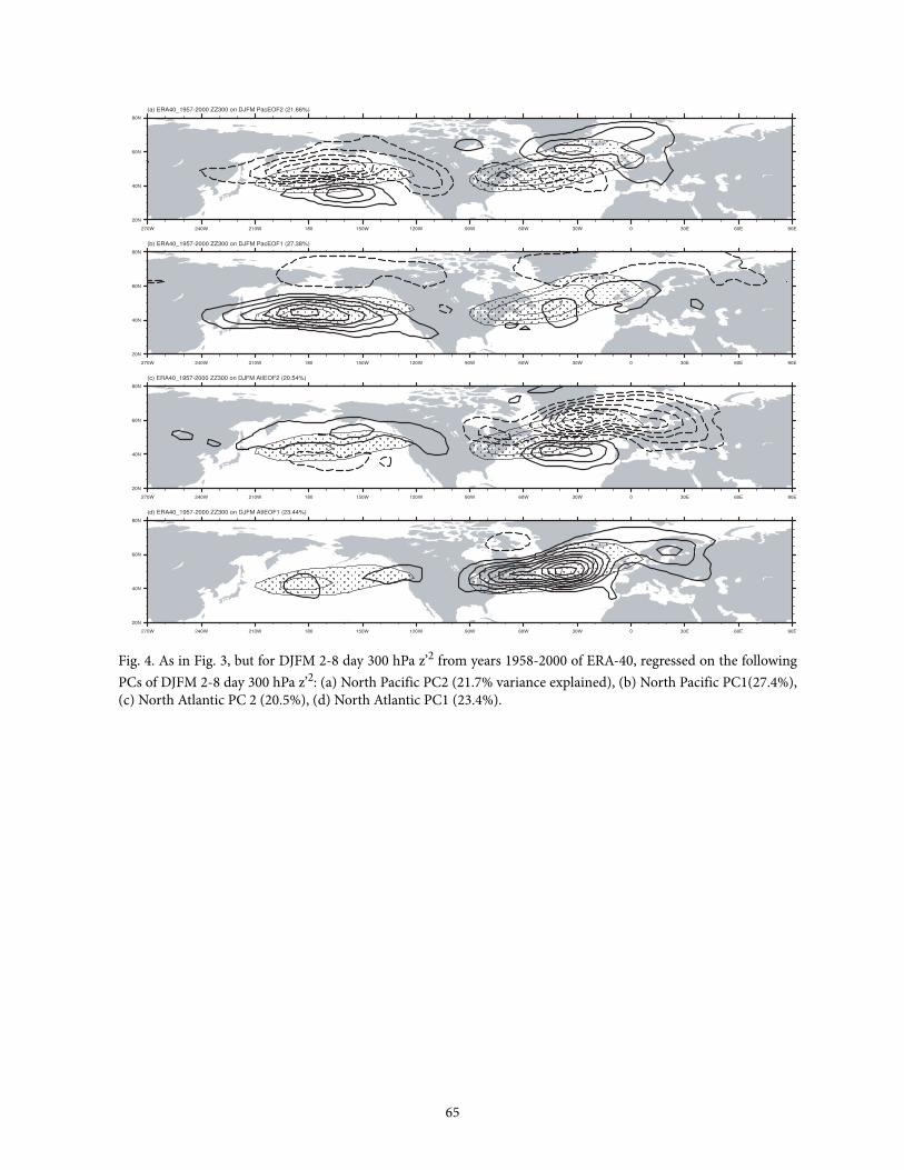
Fig. 4. As in Fig. 3, but for DJFM 2-8 day 300 hPa z’2 from years 1958-2000 of ERA-40, regressed on the following

PCs of DJFM 2-8 day 300 hPa z’2: (a) North Pacific PC2 (21.7% variance explained), (b) North Pacific PC1(27.4%),

(c) North Atlantic PC 2 (20.5%), (d) North Atlantic PC1 (23.4%).

65

Fig. 5. DJFM surface temperature, (color) and 1000 hPa zonal wind (black contours) from years 101-600 of

the CCSM3 T85 control run, regressed on the following PCs of DJFM 2-8 day 300 hPa z’2: (a) North Pacific

PC1, (b) North Pacific PC2, (c) North Atlantic PC1, (d) North Atlantic PC2. The contour interval for surface

temperature is 0.1°C, and the contour interval for 1000 hPa zonal wind is 0.5 m s-1, with the zero contour

omitted. Surface temperature is the equivalent to SST at ice free ocean grid points.

66

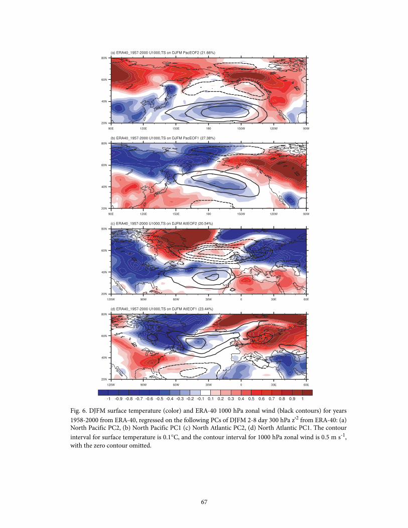
Fig. 6. DJFM surface temperature (color) and ERA-40 1000 hPa zonal wind (black contours) for years

1958-2000 from ERA-40, regressed on the following PCs of DJFM 2-8 day 300 hPa z’2 from ERA-40: (a)North Pacific PC2, (b) North Pacific PC1 (c) North Atlantic PC2, (d) North Atlantic PC1. The contour

interval for surface temperature is 0.1°C, and the contour interval for 1000 hPa zonal wind is 0.5 m s-1,

with the zero contour omitted.

67

Fig. 7. JJA surface temperature (color) and 2-8 day 300 hPa z’2 (black contours) from years 101-600 of the

CCSM3 T85 control run, regressed on the following PCs of JJA 2-8 day 300 hPa z’2: (a) North Pacific PC1(23.1% variance explained) and (c) North Atlantic PC1 (25.1%); JJA surface temperature (color) and 2-8

day 300 hPa z’2 (black contours) during years 1958-2000 from ERA-40, regressed on the following PCs of

JJA 2-8 day 300 hPa z’2 (b) North Pacific PC1 (17.2%) and (d) North Atlantic PC1 (21.7%). The contour

interval for surface temperature is 0.1°C, and the contour interval for 300 hPa z’2 is 250 m2, with the zero

contour omitted.

68

Fig. 8. Linear correlation between JJA seasonal anomalies in low-level cloud cover and SST from observations (top)and the coupled control run of CCSM3 (bottom). Observed correlations are for 1958-97 and CCSM3 correlationsare the median of twelve 40-year realizations (years100-579). Open circles mark where all realizations havecorrelations more negative than the observations and solid circles mark where all realizations have correlationsmore positive. Contour interval is 0.1, solid lines indicate negative values, dashed lines positive values, and the zeroline is thicker. Values between -0.3 and -0.5 are shaded light gray and values below -0.5 are shaded dark gray.

69

Fig. 9. As in Fig. 8, but for the correlation between low-level cloud cover and near-surface meridional wind

component. Values above 0.3 are cross-hatched.

70

Fig. 10. Correlations between interannual variations in CCSM3 monthly mean January 300 hPastreamfunction with variations in the same quantity at 33°N, 127.5°E. In this diagram as well as in Figs. 11

and 12, the effect of tropical SST anomalies has been filtered from the fields using a regression methoddescribed in the text. Also, for these same diagrams, fields have been smoothed by truncating spectrally toR15, transforming to a 48x40 Gaussian grid, and then averaging nine neighboring points. Contour intervalis 0.1.

71

Fig. 11. Correlations between interannual variations in CCSM3 monthly mean January 300 hPa streamfunction a

33°N, 127.5°E and monthly mean January variations in a) sea level pressure, b) surface temperature (which equals SST

at ocean points), c) surface latent heat flux into the atmosphere, and d) surface sensible heat flux into the atmosphere

Contour interval is 0.1.

72

Fig. 12. Correlations between interannual variations in CCSM3 monthly mean January 300 hPa streamfunction

at 33°N, 127.5°E and monthly mean surface temperature in a) February and b) March. Contour interval is 0.1.

73

Fig. 13. (a-d) SLP regimes over the North Pacific in CCSM3 during DJFM. The percentage at the top right of each

panel gives the global population of a given cluster for years 100-599. Contour interval is 2 hPa. (e-h) Simultaneous

DJFM surface temperature composites (oC) related to the four climate regimes. The events selected for the

composite construction correspond to the winters when the regime is dominant. Only significant points based on a

two-sided t-test at the 95% level are shown. Contour interval is 0.2oC.

74

Fig. 14. Same as Fig. 13 but for the regimes in the North Atlantic sector.

75

Fig 15. The observed and simulated long term mean seasonal cycle of temperature (°C, scale at bottom) and MLD

(m) in observations (top) and CCSM3 (bottom) in regions of the central North Pacific (35°N-45°N, 165°E-

175°W) and North Atlantic (50°N-60°N, 20°W-40°W). The observed temperature and MLD values are from the

World Ocean Atlas (Levitus et al. 1998) and Monterey and Levitus (1997), respectively and the model results fromyears 350-599 of CCSM3. The observed and model MLD are both based on density criteria, the former the depth

at which the density is 0.125 kg m-3 greater than at the surface and the latter is the depth of the maximumgradient that is nearest to the surface. Note that the depth scale is different in the Pacific and Atlantic plots.

76

Fig. 16: The reemergence process in the CCSM3 as indicated by lead-lag regressions (˚C per 1˚C) between

temperature anomalies at the base point, defined here as the 3 top ocean model layers (0-30 m) in FMA, and

temperature anomalies from the previous January through the following April in the (a) Pacific and (b) Atlantic

regions. The contour interval is 0.1 and values >0.5 (<0.4) in (a), and >0.8 (<0.6) in (b) are shaded light (dark).

77

Fig. 17: Basin-wide reemergence in the CCSM3 across the North Pacific (left) and North Atlantic (right)Oceans as indicated by monthly lead-lag correlations between temperature anomalies located between 65-85 min August-September, and SST anomalies from the previous January through the following April averaged over42°N-52°N. The contour interval is 0.1, and values greater than 0.55 are shaded.

78

FIg. 18: The a) observed and b) simulated PDO time series in winter, based on the leading principal component

of monthly SST anomalies north of 20oN in the Pacific, averaged over November-March. The correlation

between the wintertime PDO values and the concurrent near-surface air temperature in c) NCEP reanalysis

(1948-2003) and d) the CCSM3 (500-559).

79

120oE 140oE 160oE 180oW 160oW 140oW 120oW 100oW 20oN

30oN

40oN

50oN

60oN (a) EOF 1

(23.2 %)

5101520

25

10

1 0

10

5

5

50

00

0

0

0

0 0

120oE 140oE 160oE 180oW 160oW 140oW 120oW 100oW 20oN

30oN

40oN

50oN

60oN (b) EOF 2

(13.4 %)5

5

5

1015

20

10

10

105

5

55

5

00

0

0 0

0

0 0

Inf 20 10 6.6 5 4 3.3 2.8 2.5 2.2 2

Period (year)

0 0.05 0.1 0.15 0.2 0.25 0.3 0.35 0.4 0.45 0.5

Po

wer

Frequency (cycles/year)

(c)PC1PC2AR195%99%

Inf 20 10 6.6 5 4 3.3 2.8 2.5 2.2 2

Period (year)

Fig. 19. The (a) first and (b) second EOF of the annual mean depth of the 26.8 σθ isopycnal for years 350-599 of

the CCSM3 T85 control experiment. Values are relative to a one standard deviation change in the corresponding

PC. Contour interval is 5 m in (a) and (b). (c) Power spectrum of PC 1 and 2. Also shown are the best fit AR1

spectra and associated 95% and 99% confidence limits.

80

120oE 150oE 180oW 150oW 120oW 90oW 20oS

10oS

0o

10oN

20oN

30oN

40oN

50oN

60oN (a) EOF 1

(23.5 %)

0.2

0.2

0.20.2

0.4

10.80. 8

0.60.6 0.60.4

0.40.4

0. 40.2

0.2

0.2 0.2

0.2

0.20

0

0

0

0 00

00

0

0 0

0

00

00

0

120oE 150oE 180oW 150oW 120oW 90oW 20oS

10oS

0o

10oN

20oN

30oN

40oN

50oN

60oN (b) EOF 2

(14.0 %)

0.2

0.2

0.20.2

0.2

0.4

0.4

0.6

0.6

0.8

1

1

11.2

1.41.61.80. 2

0

0

0

0

0

0

00

00 0

0

0 0 0

Fig. 20. The (a) first (b) second EOF of the December-March mean SST for years 350-599 of the CCSM3 T85

control experiment. Values are relative to a one standard deviation change in the corresponding PC. The contour

interval is 0.2°C.

81

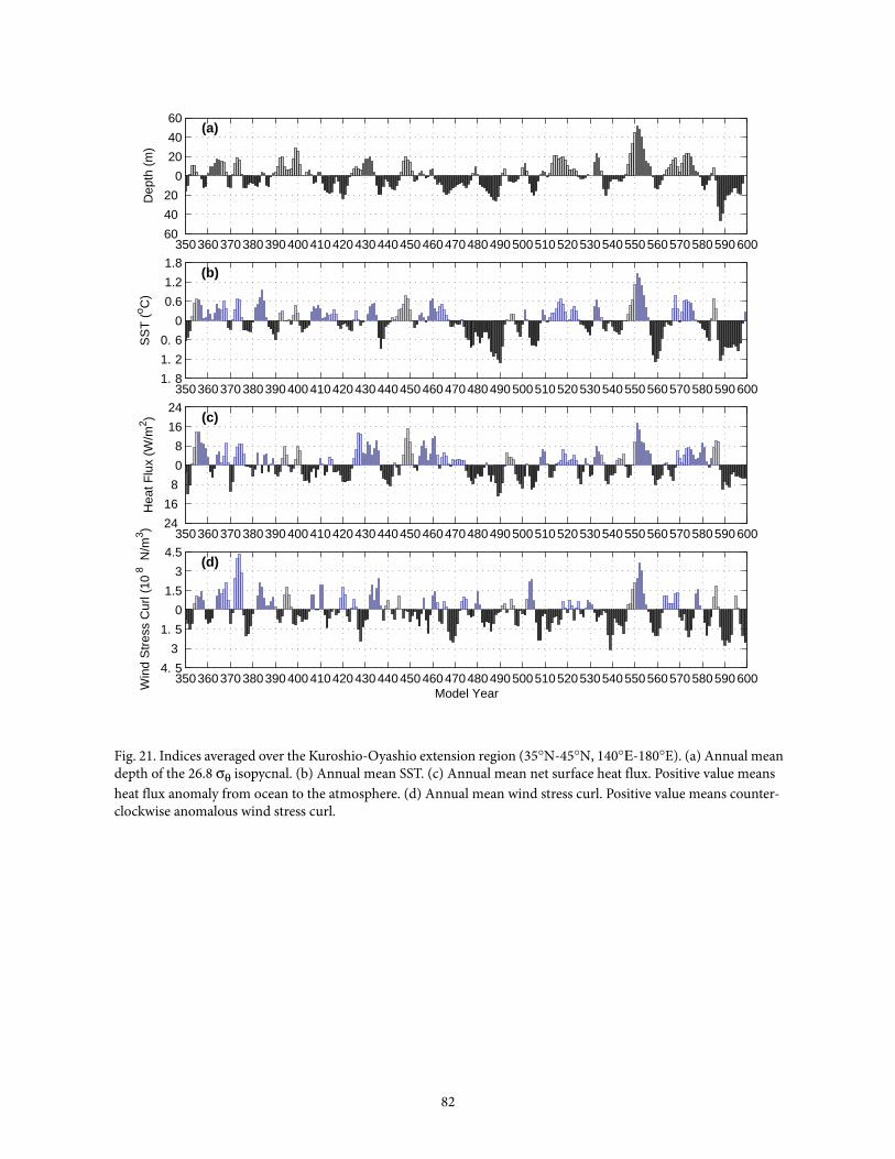
350360 370 380390 400 410420 430 440450 460 470480 490 500510 520 530540 550 560570 580 590 60060

40

20

0

20

40

60

Dep

th (

m)

(a)

350360 370 380390 400 410420 430 440450 460 470480 490 500510 520 530540 550 560570 580 590 6001. 8

1. 2

0. 6

0

0.6

1.2

1.8

SS

T (

o C)

(b)

350360 370 380390 400 410420 430 440450 460 470480 490 500510 520 530540 550 560570 580 590 60024

16

8

0

8

16

24

Hea

t Flu

x (W

/m2 ) (c)

350360 370 380390 400 410420 430 440450 460 470480 490 500510 520 530540 550 560570 580 590 6004. 5

3

1. 5

0

1.5

3

4.5

Win

d S

tres

s C

url (

108

N/m

3 )

(d)

Model Year

Fig. 21. Indices averaged over the Kuroshio-Oyashio extension region (35°N-45°N, 140°Ε-180°E). (a) Annual mean

depth of the 26.8 σθ isopycnal. (b) Annual mean SST. (c) Annual mean net surface heat flux. Positive value means

heat flux anomaly from ocean to the atmosphere. (d) Annual mean wind stress curl. Positive value means counter-

clockwise anomalous wind stress curl.

82

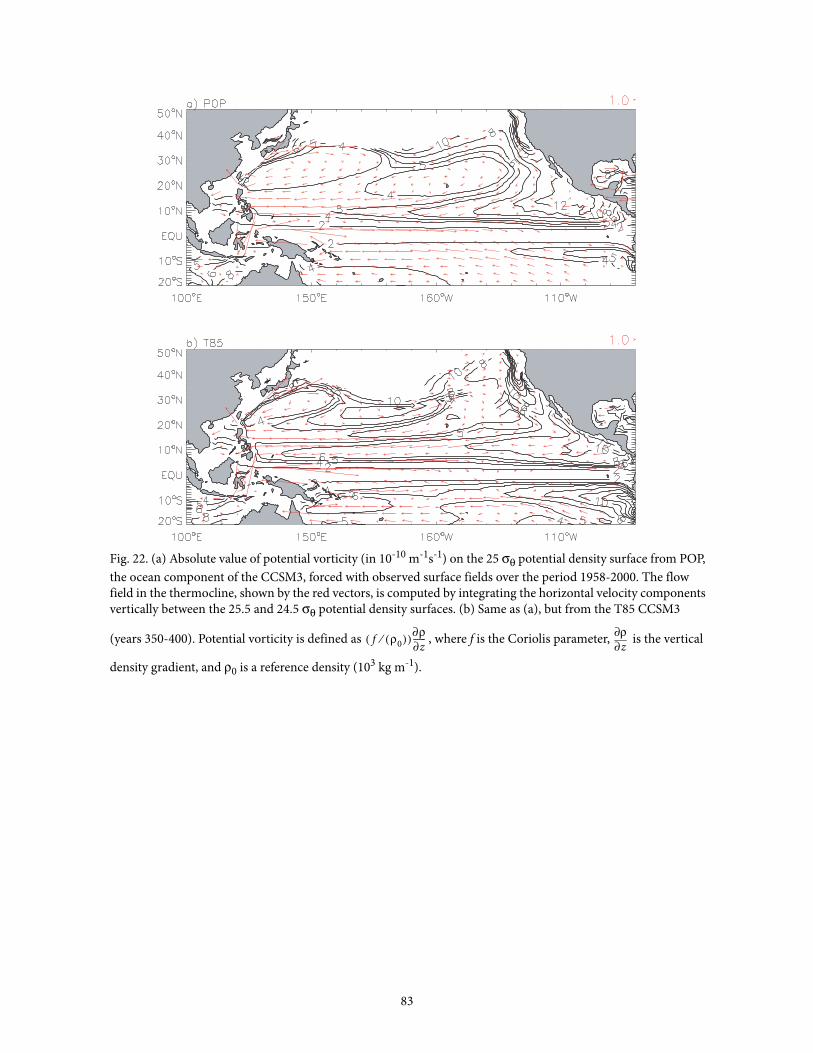
Fig. 22. (a) Absolute value of potential vorticity (in 10-10 m-1s-1) on the 25 σθ potential density surface from POP,

the ocean component of the CCSM3, forced with observed surface fields over the period 1958-2000. The flow

field in the thermocline, shown by the red vectors, is computed by integrating the horizontal velocity components

vertically between the 25.5 and 24.5 σθ potential density surfaces. (b) Same as (a), but from the T85 CCSM3

(years 350-400). Potential vorticity is defined as , where f is the Coriolis parameter, is the vertical

density gradient, and ρ0 is a reference density (103 kg m-1).

f ρ0( )⁄( )∂ρ∂z------

z∂∂ρ

83

60oW 40oW 20oW 0o 20oE

24oS

12oS

0o

12oN

24oN

60oW 40oW 20oW 0o 20oE

24oS

12oS

0o

12oN

24oN

A)

60oW 40oW 20oW 0o 20oE

24oS

12oS

0o

12oN

24oN

60oW 40oW 20oW 0o 20oE

24oS

12oS

0o

12oN

24oN B)

Fig. 23 Lagrangian trajectories along the 25.4 σθ surface in the a) POP and b) CCSM3 simulations. The trajec-

tories are based on annual averages, the triangles represent the yearly position of floats originally released at the

outcrop line in the subtropics, while the vectors indicate the direction of the flow. The trajectories are based on

the projection of the velocity field onto an isopycnal surface and, therefore, do not include diapycnal flow.

84

85

86

87