Extracting waves and vortices from Lagrangian trajectories

J. M. Lilly,1 R. K. Scott,2 and S. C. Olhede3

Received 27 September 2011; revised 25 October 2011; accepted 25 October 2011; published 7 December 2011.

[1] A method for extracting time-varying oscillatory motionsfrom time series records is applied to Lagrangian trajectoriesfrom a numerical model of eddies generated by an unstableequivalent barotropic jet on a beta plane. An oscillation in aLagrangian trajectory is represented mathematically as thesignal traced out as a particle orbits a time-varying ellipse,a model which captures wavelike motions as well as thedisplacement signal of a particle trapped in an evolvingvortex. Such oscillatory features can be separated from theturbulent background flow through an analysis foundedupon a complex-valued wavelet transform of the trajectory.Application of the method to a set of one hundred modeledtrajectories shows that the oscillatory motions of Lagrangianparticles orbiting vortex cores appear to be extracted verywell by the method, which depends upon only a handful offree parameters and which requires no operator intervention.Furthermore, vortex motions are clearly distinguished fromwavelike meandering of the jet—the former are highfrequency, nearly circular signals, while the latter are linearin polarization and at much lower frequencies. This suggeststhat the proposed method can be useful for identifying andstudying vortex and wave properties in large Lagrangiandatasets. In particular, the eccentricity of the oscillatorydisplacement signals, a quantity which is not normallyconsidered in Lagrangian studies, emerges as an informativediagnostic for characterizing qualitatively different types ofmotion. Citation: Lilly, J. M., R. K. Scott, and S. C. Olhede(2011), Extracting waves and vortices from Lagrangian trajectories,Geophys. Res. Lett., 38, L23605, doi:10.1029/2011GL049727.

1. Introduction

[2] Understanding the role of long-lived eddies in theglobal ocean circulation is a major topic in oceanographicresearch. Lagrangian floats and drifters constitute an invalu-able platform for observing the relatively small spatial andtemporal scales associated with such vortices, and indeedmany dozens of publications have examined vortex propertiesfrom regional Lagrangian experiments [e.g., Armi et al., 1989;Flament et al., 2001; Shoosmith et al., 2005]. Systematicinvestigation of the now-extensive historical set of Lagrang-ian drifter and float trajectories is, however, hampered by atechnical limitation—the lack of a reliable and precise methodto meaningfully separate vortex motions from the backgroundflow. Various approaches have been proposed [e.g., Armi

et al., 1989; Flament et al., 2001; Lankhorst, 2006]. How-ever, the fact that this problem remains unsolved is evidencedby the fact that large-scale studies either continue to rely ontraditional subjective identification [e.g., Shoosmith et al.,2005], or else to focus on measures of the effect of vorticeson trajectories rather than the properties of the vorticesthemselves [Griffa et al., 2008].[3] Recently a new and general method has been developed

[Lilly and Gascard, 2006; Lilly and Olhede, 2009a, 2009b,����@� grounded in nonstationary time series theory, whichpermits the automated identification, extraction, and analysisof time-varying oscillatory features of unknown frequency—such as the signature of a particle trapped in a vortex oradvected by a wave. Here the method is applied to Lagrangiantrajectories from a numerical simulation in order to illustratethe possibility of accurately extracting and distinguishingvortex currents and wavelike motions. All relevant analysissoftware is freely distributed to the community as a part ofa Matlab® toolbox, available at http://www.jmlilly.net.

2. Numerical Model

[4] For an idealized numerical model generating eddies aswell as background variability, we choose an equivalentbarotropic quasigeostrophic model of an initially unstable jeton a beta plane. The model integrates the equation for con-servation of potential vorticity following the geostrophicflow

!!t

! k "#F" #! "

#2F $ F=L2D ! by# $

# 0 $1%

where F is the streamfunction, b % df/dJ is the derivative ofthe Coriolis frequency f with latitude , the parameter LD is theRossby radius of deformation, and k is the vertical unitvector. The model is initialized at time t = 0 with an eastwardjet of strength U and width Y having a profile, with i beingthe eastward unit vector, given by

ujt#0 # i Ucos2 yY

p2

# $jyj=Y & 1

0 jyj=Y > 1

%$2%

which corresponds to a maximum initial vorticity anomalywithin the jet of zo % pU/(2Y).[5] Parameters are chosen to give a strong jet with a

deformation radius that is small compared to the radius ofthe earth. The central latitude (y = 0) at the jet axis is set toJ = 45° N, the jet width 2Y and deformation radius LD areboth 80 km, and the maximum initial velocity is 2.08 m s$1.These choices give a jet Rossby number Ro % zo/f = 0.80,and a value of bLD/zo of 1/(20p) & 1/60—meaning thatthe jet relative vorticity anomaly is much larger than thechange in planetary vorticity over one deformation radius,or over the jet width. This system is a convenient way

1NorthWest Research Associates, Redmond, Washington, USA.2Department of Applied Mathematics, University of St Andrews,

St Andrews, UK.3Department of Statistical Science, University College London,

London, UK.

Copyright 2011 by the American Geophysical Union.0094-8276/11/2011GL049727

GEOPHYSICAL RESEARCH LETTERS, VOL. 38, L23605, doi:10.1029/2011GL049727, 2011

L23605 1 of 5

of generating eddies, and is not intended to represent aparticular oceanic current. The initial condition is let tofreely evolve for 360 days with a time step of 5 ! 10$5 !360 days & 26 minutes in a domain of length 2p ! 400 &2500 km on each side. The model is seeded with 100 driftersthat all initially lie along the y = 0 line, sampled every 10time steps or 4.3 hours.[6] A snapshot of the model is shown in Figure 1, together

with overlays of ellipses characterizing oscillatory Lagrangianvariability from our subsequent analysis. Vortices are gener-ated by barotropic instability and then tend to drift westwardas well as meridionally due to nonlinear beta drift [e.g., Lamand Dritschel, 2001], with anticyclones propagating equa-torward and cyclones propagating poleward. Dipole interac-tions are also seen, as captured by the red/blue pair of ellipsesin the upper left quadrant of Figure 1, although these tendto eventually break down. An informative animation ofsnapshots such as the one shown in Figure 1 over the entiremodel run duration, but with the ellipses color coded bydrifter number for visual clarity, is included as a part ofthe auxiliary material.1 Trajectories are shown in Figure 2a,with the dominating presence of vortex motions apparent

as tightly looping or cycloidal curves reaching northwest-ward and southwestward.

3. Analysis Method

[7] A modulated elliptical signal, introduced by Lilly andOlhede [2010], is a time-varying oscillation in two dimen-sions. Such a signal is expressed in matrix form as

ex t$ % # cos q t$ % $sin q t$ %sin q t$ % cos q t$ %

& 'a t$ %cos ! t$ %b t$ %sin ! t$ %

& '$3%

which is the parametric equation for a particle orbiting atime-varying ellipse with semi-major and semi-minor axesa(t) and jb(t)j, where a(t) > jb(t)j > 0, and with its major axisinclined at an angle q(t) with respect to the x-axis. The phasef(t) gives the instantaneous position of the particle along theperiphery of ellipse. The particle orbits the ellipse in themathematically positive or negative direction according tothe sign of b(t).[8] Details of the modulated elliptical signal, including

conditions for associating a unique set of time-varyingellipse parameters to a given oscillatory signal ex t$ % , arediscussed by Lilly and Olhede [2010]. An important specialcase is that of a familiar pure sinusoidal oscillation in twodimensions; however, the model (3) is considerably moregeneral. A practical constraint is that the ellipse propertiesshould vary slowly compared with the timescale 2p/ddtf (t)over which the particle orbits the ellipse, in order that thesubsequent analysis method have small errors [Lilly andOlhede, ����@�[9] The modulated elliptical signal with slowly-varying

ellipse parameters is a good model for the displacementsignal of a particle trapped in an evolving vortex. This classof signals includes Lagrangian displacements due to steadycircular vortex solutions, steadily strained or sheared ellip-tical anticyclones [Ruddick, 1987], and low-frequency peri-odic oscillations of an elliptical shallow water vortex[Young, 1986; Holm, 1991], all observed with instrumentsthat may be experiencing a drift through the vortex in addi-tion to the vortex currents themselves.[10] Ellipse size, shape, and frequency are usefully char-

acterized as follows. The ellipse shape is described by theeccentricity ɛ t$ %%

((((((((((((((((((((((((((((1$b2 t$ %=a2 t$ %

p. The geometric mean

radius and geometric mean velocity are defined as

R t$ %%((((((((((((((((((a t$ %jb t$ %j

p; V t$ %%sgn bu t$ %f g

((((((((((((((((((((((au t$ %jbu t$ %j

p$4%

where the latter quantity is found by writing the velocityeu t$ %% d

dtex t$ % as a time-varying ellipse of the form (3) but witha different set of ellipse parameters, denoted au(t), bu(t), etc.;this may be accomplished algebraically from the parametersof ex t$ % , see Appendix E of Lilly and Gascard [2006]. Theratio of the two quantities V(t) and R(t) defines a frequencyv(t) % V(t)/R(t) which we call the geometric frequency.[11] A Lagrangian trajectory can then be represented as

the sum of a number M of different oscillatory displacementsignals ex mf g t$ %, each of the form (3), plus a residual:

x t$ % # x t$ %y t$ %

& '#

XM

m#1

ex mf g t$ % ! """"" t$ %: $5%

Figure 1. A snapshot of an unstable eastward equivalentbarotropic jet on a mid-latitude beta plane at day 240, withdomain details as discussed in the text. The shading is theabsolute value of the quasigeostrophic potential vorticityappearing in (1). Estimated instantaneous ellipses due toLagrangian oscillatory motions, created as in Section 3, areoverlaid. Highly eccentric ellipses with eccentricity ɛ >0.95 are shown in green, while positively-rotating and nega-tively-rotating ellipses with ɛ ' 0.95 are shown in red andblue, respectively. Dots mark the instantaneous locations of100 Lagrangian particles initially deployed along the jetaxis. Black dots indicate particles in which an oscillatorysignal is detected at this moment, while white dots indicatethe locations of other particles.

1Auxiliary materials are available in the HTML. doi:10.1029/2011GL049727.

LILLY ET AL.: WAVES AND VORTICES L23605L23605

2 of 5

The residual signal """""(t) includes the turbulent backgroundflow, as well as any non-oscillatory component such as amean flow or the systematic self-propagation tendency of avortex. The oscillatory signals may be of finite duration andmay be overlapping in time, so that zero, one, or more thanone such signal may be present at each moment.[12] The problem is then to estimate the oscillations

ex mf g t$ % given an observed trajectory x(t), and from theseestimates to characterize the M different ellipse parametersa{m}(t), b{m}(t), q{m}(t), f{m}(t), and so forth. This is accom-plished using a method called “multivariate wavelet ridgeanalysis” [Lilly and Olhede, 2009a, 2009b, ����@� leadingto estimates x̂ mf g

y t$ % of the M modulated oscillations in eachtrajectory; here the subscript “y” indicates the choice of filter

or wavelet y(t) used in the analysis. A discussion of the basicidea and implementation of the method, together with detailsof the parameter settings used here, are provided ina technical text file that is included in the auxiliary material.[13] From the method, we obtain estimates of ellipse

properties at each moment. As an example, observe the goodagreement in Figure 1 between the ellipses, inferred non-locally from individual particles, and the Eulerian structuresin the potential vorticity field.

4. Results

[14] The results of this analysis are shown in Figures 2and 3. Subtracting the sum over all M estimated oscilla-tions in each time series x(t) leads to an estimate "̂"""" t$ % of the

Figure 2. (a) All Lagrangian trajectories from the unstable barotropic jet simulation, dispersing from their initial locationat y = 0, with each trajectory in a different color. (b) The residual curves from the wavelet ridge analysis. (c, d) Snapshotsofellipses corresponding to the ellipse properties estimated from the wavelet ridge analysis. In Figures 2c and 2d, highlyeccentric ellipses with ɛ > 0.95—typically very low-frequency signals—are plotted with a time step of 1/2 the estimatedperiod, while other ellipses are plotted with the time step of every 3 estimated periods. The highly eccentric ellipses areplotted in Figure 2c in green, while the remaining anticyclonically rotating ellipses and cyclonically rotating ellipses areplotted in blue and red, respectively. Finally in Figure 2d, the ellipses are colored according to log10 of the estimatedgeometric period 2p/$(t), measured in days, as indicated in the color bar.

LILLY ET AL.: WAVES AND VORTICES L23605L23605

3 of 5

non-oscillatory background flow, Figure 2b. Comparisonwith the original time series, Figure 2a, shows that thetightly looping motions associated with vortices appear tohave been nearly completely removed. What remains behindis observed to consist of curving but disorganized motions,together with systematic motion associated with the jetand with eddy drift. Even cycloidal features in Figure 2a,typically low-frequency motion of a particle on the far flankof an eddy, are largely removed. The ability to performsuch a separation on this relative large set of drifters, withno intervention by the analyst, by itself constitutes a tech-nical breakthrough.[15] Instantaneous ellipses associated with the estimated

oscillatory signals are shown in Figures 2c and 2d. Coloringthe ellipses according to their degree of eccentricity andsense of rotation in Figure 2c reveals nearly exclusivelycyclonic motions (red) on the poleward side of the jet andanticyclonic motions (blue) on the equatorward side. Theseparation of vortices by their polarity in this system is dueto nonlinear beta drift acting on eddies generated withinthe jet core during the initial adjustment. Close inspectionreveals some very small circles of opposite color inside someof the eddies; as discussed in the technical appendix, theserepresent weak, low-frequency signals, likely associated with

the presence of exterior opposing vorticity anomalies.Another type of variability, nearly linear in polarization andoriented meridionally, is observed along the jet axis (green).[16] A time scale distinction between these two different

types of motions can be seen in Figure 2d, where the colorcoding represents the instantaneous oscillation period 2p/$(t)as deduced from the geometric frequency $(t). The highlyeccentric motions along the jet axis are seen to be an orderof magnitude lower in frequency than the vortex motions. Theformer arise as particles in the jet are swept eastward throughmeanders caused by the deflection of the jet axis by low-frequency Rossby wave variability, as is readily apparent inAnimation S1 in the auxiliary material.[17] A more detailed view of the properties of the esti-

mated elliptical signals is found in the distribution plots onthe radius/velocity plane of Figure 3. A histogram on thegeometric radius R(t)/geometric velocity V(t) plane is formedin Figure 3a by binning all time points associated with eachestimated modulated oscillation in all 100 trajectories. Notethat the slope V(t)/R(t) on this plane is the geometric fre-quency $(t). This histogram clearly reveals a Rankine-typevortex profile—a solid-body core plus 1/r decay—for cyclo-nic motions, V(t) > 0. As may be expected, the solid-bodyhistogram peak lies along the slope corresponding to the

Figure 3. Statistics of the estimated modulated elliptical signals shown on the geometric radius/velocity or R/V plane. Pos-itive and negative velocities correspond to cyclonic and anticyclonic motions respectively. (a) The histogram on the R/Vplane occupied by all estimated oscillatory signals from all 100 trajectories, with a logarithmic color axis. (b) The medianeccentricity ɛ in each bin. In Figures 3a and 3b, the sloping gray lines correspond to ±zo/2, the geometric frequency valuecorresponding (for an eddy in solid-body rotation) to the maximum initial jet relative vorticity anomaly. The black lines areplus or minus the maximum and minimum cutoff frequencies in the analysis.

LILLY ET AL.: WAVES AND VORTICES L23605L23605

4 of 5

maximum vorticity anomaly of the initial unstable jet pro-file (gray line); because under the assumption of solid-body rotation we have z = 2V/R, this occurs at a frequencyof zo/2 = 0.40f.[18] This vortex profile pattern emerges primarily through

the superposition of a number of different Lagrangian par-ticles at different locations in different eddies. On the anti-cyclonic side the pattern is less evident, since by chance,more particles have ended up in cyclonic eddies compared toanticyclonic eddies in this simulation; this asymmetry is areminder of the well-known slow convergence of Lagrangianstatistics owing to long-term particle trapping [e.g., Pasqueroet al., 2002].[19] The low-frequency motions are evident as the sym-

metric maxima in Figure 3a around the horizontal line V = 0.The median eccentricity ɛ in each bin, Figure 3b, shows thatthe motions in the vortex profile are nearly circular inpolarization, while the low-frequency motions are nearlylinear, confirming that these two regions on the R/V planecorrespond to the two types of features seen in Figures 2cand 2d. An important point is that the nearly circular vor-tex motions and the highly eccentric low-frequency motionsoccupy almost non-overlapping regions of the radius/veloc-ity plane, apart from very large-scale (say (50 km radius)and low-frequency motions, which may either be generatedby jet meander or by circular oscillatory motions on the farflank of a vortex.

5. Conclusions

[20] This paper has applied a new analysis method—multivariate wavelet ridge analysis—to the identification ofoscillatory motions in Lagrangian trajectories from anumerical simulation of an unstable jet. It is shown thatvortex motions can be effectively extracted from the trajec-tories and described locally in terms of their time-varyingfrequency content and ellipse geometry. Meridional mean-dering of the jet axis constitutes another strong oscillatorysignal in this model, but these motions are clearly distin-guished from the vortex motions on account of their muchlower frequency, nearly linear shape polarization, and dif-ferent location in radius/velocity space. The method istherefore able to unravel the superposition of different pro-cesses in individual trajectories, making possible the inves-tigation of these separate processes in isolation from oneanother. These results serve as validation supporting theapplication of this method to large-scale observational stud-ies. Not addressed here, but left to the future, are a detailedtreatment of stochastic errors, the impact of measurement

noise, comparison between the Eulerian and Lagrangianperspectives, and a consideration of method performance forother types of motions such as inertial oscillations or bar-oclinic instability waves.

[21] Acknowledgments. The work of J. M. Lilly was supported byawards #0751697 and #0849371 from the Physical Oceanography programof the United States National Science Foundation. The work of S. C. Olhedewas supported by award EP/I005250/1 from the Engineering and PhysicalSciences Research Council of the United Kingdom.[22] The Editor thanks the two anonymous reviewers for their assis-

tance in evaluating this paper.

ReferencesArmi, L., D. Hebert, N. Oakey, J. F. Price, P. Richardson, and H. Rossby

(1989), Two years in the life of aMediterranean salt lens, J. Phys. Oceanogr.,19, 354–370.

Flament, P., R. Lumpkin, J. Tournadre, and L. Armi (2001), Vortex pairingin an unstable anticyclonic shear flow: Discrete subharmonics of onependulum day, J. Fluid Mech., 440, 401–409.

Griffa, A., R. Lumpkin, and M. Veneziani (2008), Cyclonic and anti-cyclonic motion in the upper ocean, Geophys. Res. Lett., 35, L01608,doi:10.1029/2007GL032100.

Holm, D. D. (1991), Elliptical vortices and integrable Hamiltonian dynamicsof the rotating shallow-water equations, J. Fluid Mech., 227, 393–406.

Lam, J. S.-L., and D. Dritschel (2001), On the beta-drift of an intially circu-lar vortex patch, J. Fluid Mech., 436, 107–129.

Lankhorst, M. (2006), A self-contained identification scheme for eddies indrifter and float trajectories, J. Atmos. Oceanic Technol., 23, 1583–1592.

Lilly, J. M., and J.-C. Gascard (2006), Wavelet ridge diagnosis of time-varying elliptical signals with application to an oceanic eddy, NonlinearProcesses Geophys., 13, 467–483.

Lilly, J. M., and S. C. Olhede (2009a), Wavelet ridge estimation of jointlymodulated multivariate oscillations, in Conference Record of the Forty-Third Asilomar Conference on Signals, Systems, and Computers,pp. 452–456, IEEE Press, New York, doi:10.1109/ACSSC.2009.5469858.

Lilly, J. M., and S. C. Olhede (2009b), Higher-order properties of analyticwavelets, IEEE Trans. Signal Process., 57(1), 146–160, doi:10.1109/TSP.2008.2007607.

Lilly, J. M., and S. C. Olhede (2010), Bivariate instantaneous frequency andbandwidth, IEEE Trans. Signal Process., 58(2), 591–603.

Lilly, J. M., and S. C. Olhede ������� Analysis of modulated multivariateoscillations, IEEE Trans. Signal Process., in press.

Pasquero, C., A. Provenzale, and J. B. Weiss (2002), Vortex statistics fromEulerian and Lagrangian time series, Phys. Rev. Lett., 89(28), 284501.

Ruddick, B. R. (1987), Anticyclonic lenses in large-scale strain and shear,J. Phys. Oceanogr., 17, 741–749.

Shoosmith, D. R., P. L. Richardson, A. S. Bower, and H. T. Rossby (2005),Discrete eddies in the northern North Atlantic as observed by loopingRAFOS floats, Deep Sea Res., Part II, 52, 627–650.

Young, W. R. (1986), Elliptical vortices in shallow water, J. Fluid Mech.,171, 101–119.

J. M. Lilly, NorthWest Research Associates, 4118 148th Ave. NE,Redmond, WA 98052, USA. (lilly@nwra.com)S. C. Olhede, Department of Statistical Science, University College

London, Gower Street, London WC1E 6BT, UK.R. K. Scott, Department of Applied Mathematics, University of St Andrews,

St Andrews KY16 9SS, UK.

LILLY ET AL.: WAVES AND VORTICES L23605L23605

5 of 5

GEOPHYSICAL RESEARCH LETTERS, VOL. ???, XXXX, DOI:10.1029/,

Text S1

The extraction of individual oscillatory signals from the modeled Lagrangian trajectories

is accomplished using a method called “multivariate wavelet ridge analysis” [Lilly and

Olhede, 2009a, 2011]. All numerical code associated with this paper is distributed as

part of a Matlab R! toolbox called Jlab, available at http://www.jmlilly.net. The file

makefigs vortex provides the exact processing steps as well as scripts to generate all

figures. This file describes the basic idea and presents an example. Equation numbers

herein refer to the main text.

An analytic wavelet is a time/frequency localized filter which has vanishing support on

negative Fourier frequencies, and which is therefore complex-valued in the time domain,

see e.g. Lilly and Olhede [2009b] and references therein for details. The wavelet transform

of a real-valued signal vector x(t) with respect to the wavelet !(t) is defined as

wx,!(t, s) "! !

"!

1

s!#

"" # t

s

#x(") d"

and can be seen, on account of the 1/s normalization, as a set of bandpass operations

indexed by the “scale” s which controls the dilation or contraction of the wavelet in time.

The frequency-domain wavelet !(#) obtains a maximum magnitude, set to !(#) = 2, at

some frequency #!. This frequency is used to convert scale into a period via 2$s/#!.

D R A F T November 3, 2011, 11:08am D R A F T

X - 2 LILLY ET AL.: TEXT S1

The particular choice of analyzing wavelet !(t) is important in order to minimize errors

in the subsequent analysis [Lilly and Olhede, 2009b, 2011]. We use the “Airy wavelet”

of Lilly and Olhede [2009b], which can be seen as a superior alternative to the popular

but problematic Morlet wavelet, as discussed therein. The Airy wavelet is controlled by a

parameter P!, with P!/$ giving the number of oscillations spanning the central window

of the wavelet. We choose P!/$ =$6/$ % 0.78 in order to obtain a high degree of time

concentration at the expense of frequency resolution.

Multivariate wavelet ridge analysis estimates modulated oscillations in a multivariate,

or vector-valued, time series by first identifying maxima of the transform magnitude. A

brief introduction to this method may be found in Lilly and Olhede [2009a], with further

details and bias estimates provided by Lilly and Olhede [2011]. A ridge point of wx,!(t, s)

is defined to be a point on the (t, s) or “time/scale” plane satisfying

%

%s&wx,!(t, s)& = 0,

%2

%s2&wx,!(t, s)& < 0

and thus ridge points are locations where the norm of the wavelet transform vector achieves

a local maximum with respect to variations in scale. Adjacent ridge points are then

connected to each other to yield a single-valued, continuous scale curve as a function of

time called a ridge $s(t).

A number, say M , di"erent ridges $s{m}(t) may be present in the same time series, and

may overlap in time. The real part of the wavelet transform along the mth ridge may

be taken as an estimate of the mth oscillatory signal %x{m}(t) in the composite model (5).

That is

$x{m}! (t) " '

&wx,!

't, $s{m}(t)

()= %x{m}(t) +#%x{m}

! (t)

D R A F T November 3, 2011, 11:08am D R A F T

LILLY ET AL.: TEXT S1 X - 3

where the last term on the right-hand side is an error term. This may be understood as

resulting from the fact that the real part of the wavelet transform at scale s = #!/# is a

bandpass at frequency #; thus the wavelet ridge estimate combines di"erent pass bands at

di"erent times, as is appropriate for the time-varying nature of the signal. The error term

depends upon several factors: (i) the local ratio of the oscillatory signal strength to the

background variability strength, (ii) the magnitude of changes in oscillation properties

over the wavelet timescale, see the treatment in Lilly and Olhede [2011], and (iii) the

distance between contemporaneous oscillatory signals in frequency compared with the

wavelet frequency profile. A detailed treatment of errors is outside the scope of this

paper; instead, we will point to Fig. 2b in the text and the example below as subjective

evidence that oscillatory signals have been recovered satisfactorily.

It remains to form estimates of the ellipse parameters in the modulated elliptical signal

model (3) associated with each of the M ridges. Observe that, as there are two param-

eters on the left-hand side of (3) but four parameters on the right-hand side, the ellipse

parameters are underdetermined for a given oscillatory signal %x(t). Since the analytic

wavelet transform wx,!(t, s) is a complex-valued 2-vector, it consists of four quantities at

each time. It has been shown by Lilly and Gascard [2006] and Lilly and Olhede [2010]

that the complex-valued wavelet transform evaluated along the ridge may be written as

wx,!

't, $s{m}(t)

(= ei

!"{m}(t)

*cos $&{m}(t) # sin $&{m}(t)

sin $&{m}(t) cos $&{m}(t)

+ ,$a{m}(t)

#i$b{m}(t)

-

with the four quantities on the right-hand side being the sought-after estimates of the

four ellipse parameters at each moment for each ridge. The “hats” mark estimated ellipse

parameters that are defined implicitly through this equation.

D R A F T November 3, 2011, 11:08am D R A F T

X - 4 LILLY ET AL.: TEXT S1

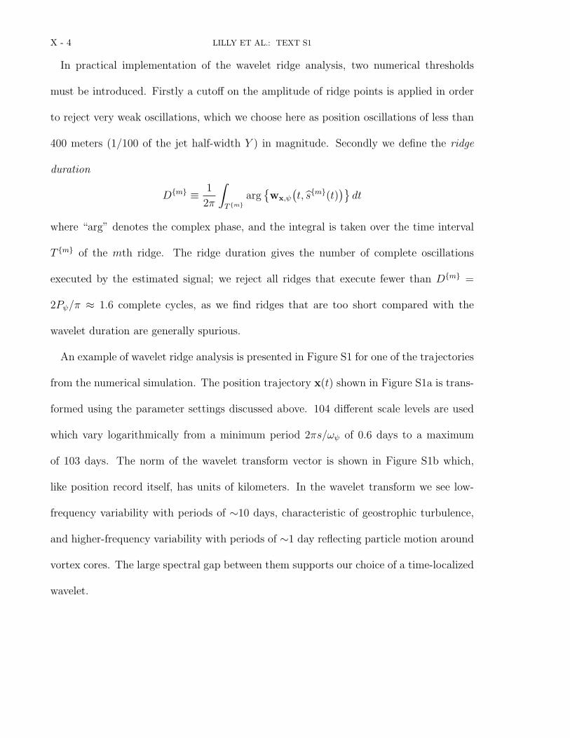
In practical implementation of the wavelet ridge analysis, two numerical thresholds

must be introduced. Firstly a cuto" on the amplitude of ridge points is applied in order

to reject very weak oscillations, which we choose here as position oscillations of less than

400 meters (1/100 of the jet half-width Y ) in magnitude. Secondly we define the ridge

duration

D{m} " 1

2$

!

T {m}arg

&wx,!

't, $s{m}(t)

()dt

where “arg” denotes the complex phase, and the integral is taken over the time interval

T {m} of the mth ridge. The ridge duration gives the number of complete oscillations

executed by the estimated signal; we reject all ridges that execute fewer than D{m} =

2P!/$ % 1.6 complete cycles, as we find ridges that are too short compared with the

wavelet duration are generally spurious.

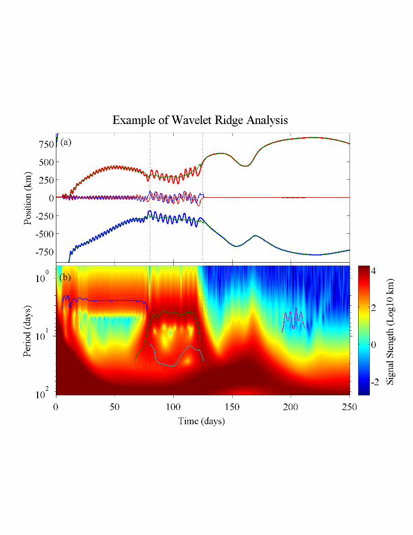
An example of wavelet ridge analysis is presented in Figure S1 for one of the trajectories

from the numerical simulation. The position trajectory x(t) shown in Figure S1a is trans-

formed using the parameter settings discussed above. 104 di"erent scale levels are used

which vary logarithmically from a minimum period 2$s/#! of 0.6 days to a maximum

of 103 days. The norm of the wavelet transform vector is shown in Figure S1b which,

like position record itself, has units of kilometers. In the wavelet transform we see low-

frequency variability with periods of (10 days, characteristic of geostrophic turbulence,

and higher-frequency variability with periods of (1 day reflecting particle motion around

vortex cores. The large spectral gap between them supports our choice of a time-localized

wavelet.

D R A F T November 3, 2011, 11:08am D R A F T

LILLY ET AL.: TEXT S1 X - 5

M = 4 ridges are detected and are marked in the figure as curves indicating maxima of

the wavelet transform with respect to scale. The real part of the wavelet transform along

the mth ridge estimates the mth oscillatory signal component in the composite model (5),

which the analysis is able to isolate from the surrounding variability. These four estimated

signals are then plotted in Figure S1a along with the residuals. It is observed that the

oscillatory features in the original trajectory are removed extremely well by the analysis

method.

In the central part of the record, two ridges are simultaneously present, with the lower-

frequency curve representing an interaction with a distant vortex. A very weak amplitude

ridge, just greater than our cuto" amplitude, is detected near the end of the time series;

this is almost certainly spurious and illustrates the reason why we impose an amplitude

cuto"; weak “false positives” such as this signal do not impact our analysis because

their amplitude is so small, and because they appear to occur rarely. Note that the

low-frequency background, while slowly meandering in nature, does not generate ridges

because it does not typically result in the appearance of multiple orbits through the same

oscillatory structure, and is therefore not characterized as a modulated oscillation by this

analysis.

There are two transitions in this time series: one around 80 days, when the main ridge

lowers its frequency and a second contemporaneous ridge appears, and a second transition

around 125 days, when these two ridges disappear. It can be seen from watching the

animation, also included in the auxilary materials, that these two transitions correspond

to two vortex mergers. In that animation, ellipses associated with this trajectory are drawn

D R A F T November 3, 2011, 11:08am D R A F T

X - 6 LILLY ET AL.: TEXT S1

in black, and the position of this drifter is indicated with a magenta dot. During the first

merger, the vortex grows in size and its frequency decreases, but there is a remaining

distant vortex which causes lower-frequency oscillatory motion that is manifested as the

lower of the two ridges. During the second merger, the particle is ejected in a filament

and consequently the oscillatory motions come to an end. This indicates that transitions

in the ridges can have physical meaning and can capture vortex evolution.

References

Armi, L., D. Hebert, N. Oakey, J. F. Price, P. Richardson, and H. Rossby, Two years in

the life of a Mediterranean salt lens, J. Phys. Oceanogr., 19, 354–370, 1989.

Flament, P., R. Lumpkin, J. Tournadre, and L. Armi, Vortex pairing in an unstable

anticyclonic shear flow: discrete subharmonics of one pendulum day, J. Fluid Mech.,

440, 401–409, 2001.

Gri"a, A., R. Lumpkin, and M. Veneziani, Cyclonic and anticyclonic motion in the upper

ocean, Geophys. Res. Lett., 35, L01,608, 2008.

Holm, D. D., Elliptical vortices and integrable Hamiltonian dynamics of the rotating

shallow-water equations, J. Fluid Mech., 227, 393–406, 1991.

Lam, J. S.-L., and D. Dritschel, On the beta-drift of an intially circular vortex patch, J.

Fluid Mech., 436, 107–129, 2001.

Lankhorst, M., A self-contained identification scheme for eddies in drifter and float tra-

jectories, J. Atmos. Ocean Tech., 23, 1583–1592, 2006.

Lilly, J. M., and J.-C. Gascard, Wavelet ridge diagnosis of time-varying elliptical signals

with application to an oceanic eddy, Nonlinear Proc. Geoph., 13, 467–483, 2006.

D R A F T November 3, 2011, 11:08am D R A F T

LILLY ET AL.: TEXT S1 X - 7

Lilly, J. M., and S. C. Olhede, Wavelet ridge estimation of jointly modulated multivariate

oscillations, in 2009 Conference Record of the Forty-Third Asilomar Conference on Sig-

nals, Systems, and Computers, pp. 452–456, doi:10.1109/ACSSC.2009.5469858, 2009a.

Lilly, J. M., and S. C. Olhede, Higher-order properties of analytic wavelets, IEEE T.

Signal Proces., 57 (1), 146–160, doi:10.1109/TSP.2008.2007607, 2009b.

Lilly, J. M., and S. C. Olhede, Bivariate instantaneous frequency and bandwidth, IEEE

T. Signal Proces., 58 (2), 591–603, 2010.

Lilly, J. M., and S. C. Olhede, Analysis of modulated multivariate oscillations, IEEE T.

Signal Proces., accepted., 2011.

Pasquero, C., A. Provenzale, and J. B. Weiss, Vortex statistics from Eulerian and La-

grangian time series, Phys. Rev. Lett., 89 (28), 284,501–1–284,501–4, 2002.

Ruddick, B. R., Anticyclonic lenses in large-scale strain and shear, J. Phys. Oceanogr.,

17, 741–749, 1987.

Shoosmith, D. R., P. L. Richardson, A. S. Bower, and H. T. Rossby, Discrete eddies in

the northern North Atlantic as observed by looping RAFOS floats, Deep-Sea Res. Pt.

II, 52, 627–650, 2005.

Young, W. R., Elliptical vortices in shallow water, J. Fluid Mech., 171, 101–119, 1986.

D R A F T November 3, 2011, 11:08am D R A F T

X - 8 LILLY ET AL.: TEXT S1

Figure S1. An illustration of wavelet ridge analysis. In (a), the east–west and north–south

displacement signals associated with a Lagrangian “particle” in the model simulation are shown

with the blue and red heavy lines, respectively. Thin blue and red lines show aggregate east–

west and north–south oscillatory displacement signals obtained by summing over all estimated

modulated oscillations $x{m}! (t) at each time. The green curves are the east–west and north–south

residuals x(t) #.M

m=1 $x{m}! (t). The wavelet transform norm &wx,!(t, s)& is shown in (b), with

scale converted into period on the y-axis. Four ridge curves are identified and drawn. The real

part of the wavelet transform evaluated along these four curves give the estimated oscillations

used in panel (a). Vertical lines in both panels mark the approximate times of vortex merger

events as seen in the animation.

D R A F T November 3, 2011, 11:08am D R A F T