Extracting Surface Structural Information from Vibrational Spectra ...

Extracting Surface Structural Information from Vibrational Spectra with LinearProgramming

by

Kuo Kai HungB.Sc., University of Victoria, 2012

A thesis submitted in Partial Fulfillment of theRequirements for the Degree of

MASTER OF SCIENCE

in the Department of Computer Science

c© Kuo Kai Hung, 2015University of Victoria

All rights reserved. This thesis may not be reproduced in whole or in part,by photocopying or other means, without the permission of the author.

ii

Extracting Surface Structural Information from Vibrational Spectra with LinearProgramming

by

Kuo Kai HungB.Sc., University of Victorial, 2012

Supervisory committee

Dr. Dennis K. Hore, Co-Supervisor(Department of Chemistry)

Dr. Ulrike Stege, Co-Supervisor(Department of Computer Science)

iii

Dr. Dennis K. Hore, Co-Supervisor(Department of Chemistry)

Dr. Ulrike Stege, Co-Supervisor(Department of Computer Science)

ABSTRACT

Vibrational spectra techniques such as IR, Raman and SFG all carry molecular orientation

information. Extracting the orientation information from the vibrational spectra often

involves creating model spectra with known orientation details to match the experimental

spectra. The running time for the exhaustive approach is O(n!). With the help of linear

programming, the running time is pseudo O(n). The linear programming approach is

with out a doubt far more superior than exhaustive approach in terms of running time.

We verify the accuracy of the answer of the linear programming approach by creating

mock experimental data with known molecular orientation distribution information of

alanine, isoleucine, methionine, lysine, valine and threonine. Linear programming returns

the correct orientation distribution information when the mock experimental spectrum

consisted of different amino acids. As soon as the mock experimental spectrum consisted

of same amino acids, different conformer with different orientation distribution, linear

programming fails to give the correct answer albeit the species population is roughly

correct.

iv

Contents

Supervisory Committee . . . . . . . . . . . . . . . . . . . . . . . . . . . . . . . ii

Abstract . . . . . . . . . . . . . . . . . . . . . . . . . . . . . . . . . . . . . . . iii

Table of contents . . . . . . . . . . . . . . . . . . . . . . . . . . . . . . . . . . iv

List of figures . . . . . . . . . . . . . . . . . . . . . . . . . . . . . . . . . . . . vii

List of tables . . . . . . . . . . . . . . . . . . . . . . . . . . . . . . . . . . . . . xiii

List of symbols and definitions . . . . . . . . . . . . . . . . . . . . . . . . . . . xiv

Acknowledgments . . . . . . . . . . . . . . . . . . . . . . . . . . . . . . . . . . xv

1 Introduction 1

1.1 Background and Motivation . . . . . . . . . . . . . . . . . . . . . . . . . 1

1.1.1 Infrared absorption spectra . . . . . . . . . . . . . . . . . . . . . . 5

1.1.2 Raman scattering spectra . . . . . . . . . . . . . . . . . . . . . . . 5

1.1.3 Vibrational sum-frequency spectra . . . . . . . . . . . . . . . . . . 6

1.2 Aims and Scope . . . . . . . . . . . . . . . . . . . . . . . . . . . . . . . . 7

2 Methods 9

2.1 Vibrational Spectrum simulation overview . . . . . . . . . . . . . . . . . . 9

2.2 Coordinate transformation . . . . . . . . . . . . . . . . . . . . . . . . . . 11

2.2.1 Unit Vectors in the lab and molecular frames . . . . . . . . . . . . 11

2.2.2 Direction cosine matrix . . . . . . . . . . . . . . . . . . . . . . . . 13

2.2.3 Obtaining the Euler angles . . . . . . . . . . . . . . . . . . . . . . 14

2.3 Projecting molecular properties into the lab frame . . . . . . . . . . . . . . 17

v

2.3.1 Infrared absorption spectra . . . . . . . . . . . . . . . . . . . . . . 17

2.3.2 Raman scattering spectra . . . . . . . . . . . . . . . . . . . . . . . 18

2.3.3 Vibrational sum-frequency spectra . . . . . . . . . . . . . . . . . . 19

2.4 Orientation distribution . . . . . . . . . . . . . . . . . . . . . . . . . . . . 20

2.4.1 Numerical method - Molecular Dynamic (MD) Simulation . . . . . 21

2.4.2 Analytic method - Gaussian Distribution . . . . . . . . . . . . . . 22

3 Sensitivity of different techniques to orientation distribution 23

3.1 Overview . . . . . . . . . . . . . . . . . . . . . . . . . . . . . . . . . . . 23

3.2 Formalism and molecular response . . . . . . . . . . . . . . . . . . . . . . 23

3.2.1 Vibrational Response . . . . . . . . . . . . . . . . . . . . . . . . . 23

3.2.2 Molecular orientation distribution . . . . . . . . . . . . . . . . . . 24

3.3 Results and discussion . . . . . . . . . . . . . . . . . . . . . . . . . . . . 27

3.3.1 Vibrational modes dominated by a single element in the IR and

Raman response . . . . . . . . . . . . . . . . . . . . . . . . . . . 27

3.3.2 Methyl group response . . . . . . . . . . . . . . . . . . . . . . . . 32

3.3.3 Numerical orientation distributions . . . . . . . . . . . . . . . . . 40

3.4 Conclusions . . . . . . . . . . . . . . . . . . . . . . . . . . . . . . . . . . 42

4 Linear Programming 44

4.1 Overview . . . . . . . . . . . . . . . . . . . . . . . . . . . . . . . . . . . 44

4.2 Introduction . . . . . . . . . . . . . . . . . . . . . . . . . . . . . . . . . . 44

4.3 Linear Programming with inequality constraints . . . . . . . . . . . . . . . 49

4.4 Generating the candidates . . . . . . . . . . . . . . . . . . . . . . . . . . . 51

4.5 Combining the candidates . . . . . . . . . . . . . . . . . . . . . . . . . . . 55

4.6 Differential weighting of candidate sampling points . . . . . . . . . . . . . 59

4.7 GNU linear programming tool kit . . . . . . . . . . . . . . . . . . . . . . 60

4.8 Methods and Implementation . . . . . . . . . . . . . . . . . . . . . . . . . 62

vi

4.8.1 Making SFG pickle files for linear programming . . . . . . . . . . 62

4.8.2 The experimental data file . . . . . . . . . . . . . . . . . . . . . . 63

4.8.3 Linear Programming Text Input . . . . . . . . . . . . . . . . . . . 63

4.8.4 Linear Programming Input and Output . . . . . . . . . . . . . . . . 64

4.8.5 Plotting Result . . . . . . . . . . . . . . . . . . . . . . . . . . . . 64

4.9 Results and Discussion . . . . . . . . . . . . . . . . . . . . . . . . . . . . 65

4.9.1 Delta distributions . . . . . . . . . . . . . . . . . . . . . . . . . . 65

4.9.2 Gaussian distribution, theta only . . . . . . . . . . . . . . . . . . . 68

4.9.3 Discussion . . . . . . . . . . . . . . . . . . . . . . . . . . . . . . 70

4.10 Conclusions . . . . . . . . . . . . . . . . . . . . . . . . . . . . . . . . . . 72

5 Summary and future work 77

5.1 Summary . . . . . . . . . . . . . . . . . . . . . . . . . . . . . . . . . . . 77

5.2 Future work . . . . . . . . . . . . . . . . . . . . . . . . . . . . . . . . . . 78

vii

List of Figures

1.1 Various systems that may be probed with vibrational spectroscopy in-

cluding the (a) air/vacuum–solid surface, (b) solid–water interface, (c)

molecules in solution, adsorbed at the solid–solution interface, (d) dried

samples, measured at the air/vacuum–solid surface, and (e) rinsed samples,

measured at the solid–water interface. In each case, IR absorption

spectroscopy, Raman scattering, and/or SFG spectroscopy may be used,

depending on the focus of the study. . . . . . . . . . . . . . . . . . . . . . 4

2.1 Illustration of vectors that may be used to define the molecular-frame

unit vectors for a water molecule. (a) In the case where both O–H bond

lengths are known to be fixed and equal, one can define ~c as the vector

that runs from the midpoint M of the two H atoms to the O atom. ~a is

then simply defined between the two H atoms. (b) In the case where the

bond lengths may be unequal, it may be simpler to define ~a first, between

the two H atoms. ~c would then originate from a point P along ~a, such

that the vector defined between P and the O atom is perpendicular to ~a.

These decisions should follow from whatever is most clear or logical for a

particular molecule. In both cases, ~b may be obtained in the last step from

the cross product relationship between the unit vectors in a right-handed

coordinate system. . . . . . . . . . . . . . . . . . . . . . . . . . . . . . . 12

2.2 The Euler angles represented as the spherical polar angles θ, φ and ψ. . . . 15

viii

2.3 Illustration of the 3 successive rotations that transform the lab (x, y, z)

coordinate system into the molecular (a, b, c) frame. In the case of an

intrinsic set of rotations (top row), one performs Rz(φ) a rotation by φ

about z, Ry′(θ) rotation by θ about y′, and finally Rc(ψ) rotation by ψ

about c. In the case of an extrinsic set of rotations (bottom row), one

performs Rz(ψ) a rotation by ψ about z, Ry(θ) rotation by θ about y, and

finally Rz(φ) rotation by φ about z. . . . . . . . . . . . . . . . . . . . . . 15

3.1 The x and z components of the IR absorption (first row), xx, xy, xz,

and zz components of the Raman scattering (middle row), and xxz, xzx,

and zzz components of the hyperpolarizability (bottom row) for a uniaxial

vibrational mode as a function of the mean tilt angle θ0 and half-width σ of

a Gaussian distribution of the methyl C3 axes. Darker red colors indicate

higher intensity. Horizontal dashed white lines at σ = 7.5 and σ = 50

indicate distribution widths for which derivatives are displayed in Fig. 3.2. . 29

3.2 Derivatives of the uniaxial response function plotted in Fig. 3.1 correspond-

ing to a narrow distribution with σ = 7.5 (a) The solid green line indicates

the slope of x with respect to θ0; the dashed green line z. (b) Similarly, the

slopes of the Raman response are indicated in red, with the solid lines for

xx, short dashes xy, medium dashes xz, and long dashes zz. (c) Finally

the slope of the SFG response with respect to θ0 is indicated in blue, with

the solid line corresponding to xxz, short dashes xzx, and medium dashes

zzz. The second column illustrates a wide distribution with σ = 50 for

the (d) IR, (e) Raman, and (f) SFG response. . . . . . . . . . . . . . . . . . 31

ix

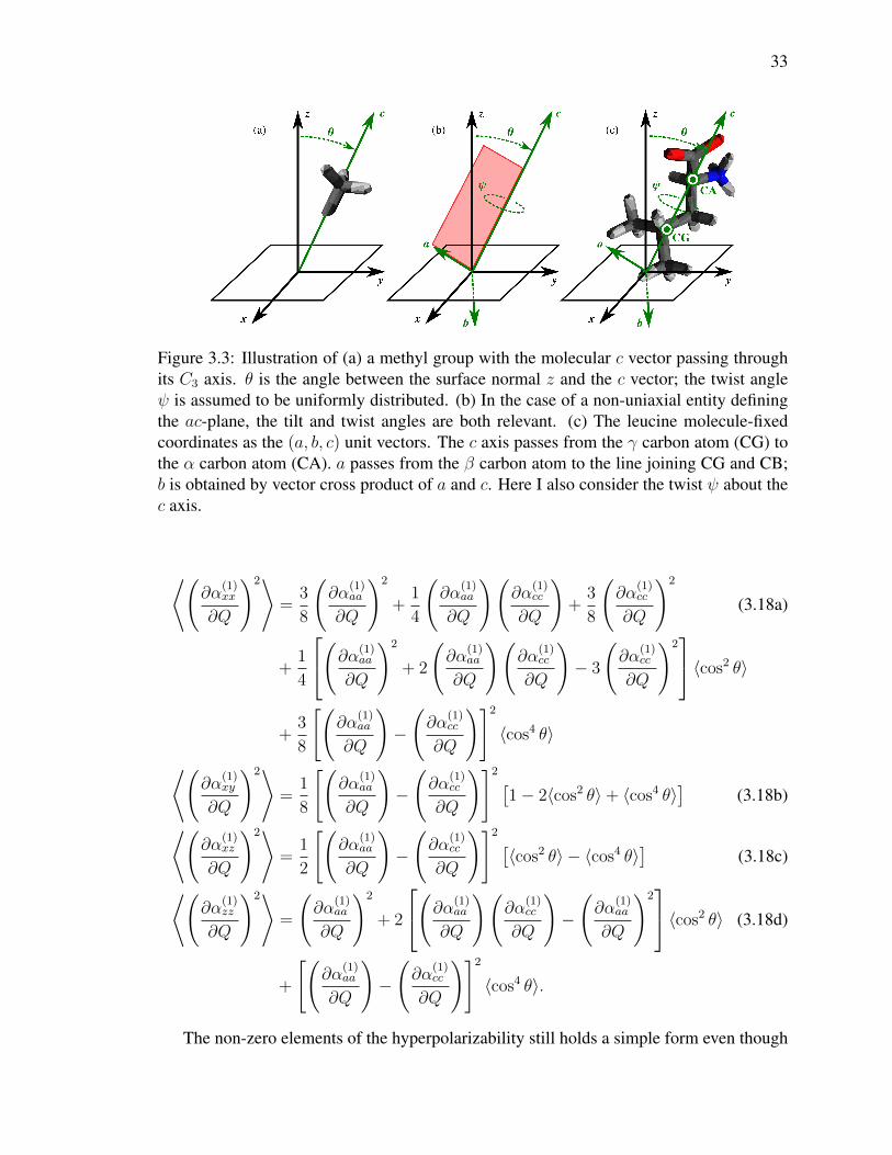
3.3 Illustration of (a) a methyl group with the molecular c vector passing

through its C3 axis. θ is the angle between the surface normal z and the

c vector; the twist angle ψ is assumed to be uniformly distributed. (b) In

the case of a non-uniaxial entity defining the ac-plane, the tilt and twist

angles are both relevant. (c) The leucine molecule-fixed coordinates as the

(a, b, c) unit vectors. The c axis passes from the γ carbon atom (CG) to the

α carbon atom (CA). a passes from the β carbon atom to the line joining

CG and CB; b is obtained by vector cross product of a and c. Here I also

consider the twist ψ about the c axis. . . . . . . . . . . . . . . . . . . . . . 33

3.4 The x and z components of the IR absorption (first row), xx, xy, xz,

and zz components of the Raman scattering (middle row), and xxz, xzx,

and zzz components of the hyperpolarizability (bottom row) for a methyl

symmetric stretch as a function of the mean tilt angle θ0 and half-width

σ of a Gaussian distribution of the methyl C3 axes. Eight combinations

A–H of the parameters θ0 and σ in the Gaussian distribution are shown as

annotations on the plots for comparison with Fig. 3.6 and Fig. 3.7. Positive

values are shaded in red with solid contours; negative values are shaded in

blue with dashed contours. Horizontal dashed white lines at σ = 7.5 and

σ = 50 indicate distribution widths for which derivatives are displayed in

Fig. 3.5. . . . . . . . . . . . . . . . . . . . . . . . . . . . . . . . . . . . . 35

x

3.5 Derivatives of the uniaxial response function plotted in Fig. 3.4 correspond-

ing to a narrow distribution with σ = 7.5 (a) The solid green line indicates

the slope of x with respect to θ0; the dashed green line z. (b) Similarly, the

slopes of the Raman response are indicated in red, with the solid lines for

xx, short dashes xy, medium dashes xz, and long dashes zz. (c) Finally

the slope of the SFG response with respect to θ0 is indicated in blue, with

the solid line corresponding to xxz, short dashes xzx, and medium dashes

zzz. The second column illustrates a wide distribution with σ = 50 for

the (d) IR, (e) Raman, and (f) SFG response. . . . . . . . . . . . . . . . . . 37

3.6 The aliphatic stretching spectra of leucine for 4 combinations A–D of

the parameters θ0 and σ representing wide Gaussian distributions of tilt

angles. Model IR absorption x and z spectra are shown in the top row.

Raman xx, xy, xz, and zz scattering spectra are displayed in the middle

row. The imaginary component of the complex-valued xxz, xzx, and

zzz χ(2) spectra corresponding to a visible-IR sum-frequency generation

experiment are shown in the bottom row. . . . . . . . . . . . . . . . . . . . 39

3.7 The aliphatic stretching spectra of leucine for 4 combinations E–H of the

parameters θ0 and σ representing relatively narrow Gaussian distributions

of tilt angles. Model IR absorption x and z spectra are shown in the top row.

Raman xx, xy, xz, and zz scattering spectra are displayed in the middle

row. The imaginary component of the complex-valued xxz, xzx, and

zzz χ(2) spectra corresponding to a visible-IR sum-frequency generation

experiment are shown in the bottom row. . . . . . . . . . . . . . . . . . . . 40

xi

3.8 The aliphatic stretching spectra of leucine obtained from molecular dy-

namics simulations of adsorption from solution onto two types of surfaces.

Results for a superhydrophobic surface (contact angle ≈ 150) are shown

in blue; results for a moderately hydrophobic surface (contact angle≈ 85)

are shown in red. Model IR absorption x and z spectra are shown in the

top row. Raman xx, xy, xz, and zz scattering spectra are displayed in

the middle row. The imaginary component of the complex-valued xxz,

xzx, and zzz. χ(2) spectra corresponding to a visible-IR sum-frequency

generation experiment are shown in the bottom row. . . . . . . . . . . . . . 41

4.1 These are three figures to help explain the idea of sum of difference. A is

the target. B and C are candidates. Three points selected in each figure to

perform sum of difference. . . . . . . . . . . . . . . . . . . . . . . . . . . 45

4.2 These are three figures to help explain the idea of sum of squared

difference. A is the target. B and C are candidate. Three points selected in

each figure to perform sum of squared difference. . . . . . . . . . . . . . . 47

4.3 All the possible solutions that satisfies the constraints are inside the gray

area. The optimum solution happens at the vertices. . . . . . . . . . . . . . 49

4.4 The imaginary component of alaine’s ssp response. Blue line represent

alanie with orientation distribution of θ0 = 60 and θσ = 30. Green line

represents alanine with orientation distribution of θ0 = 30 and θσ = 5 . . 56

4.5 The top panel show the spectrum that linear programming returns. The bot-

tom panel show the difference between the result that linear programming

returns and the actual spectrum. . . . . . . . . . . . . . . . . . . . . . . . 66




xii




4.8 Linear programming solver does not return the optimal solution. The

bottom panel show the difference at each data point. As one can see, there

are some difference at some data points. This indicates the returned answer

is not perfect. . . . . . . . . . . . . . . . . . . . . . . . . . . . . . . . . . 69

4.9 The vertical axis is θ0. The saturation of the color is representative of the

difference in shape between θσ = 5 and θσ = 30 for that particular θ0 of

alanine. The first three panels represents the difference for ssp, sps and ppp

respectively. The bottom panel shows the difference considering all three

polarizations. . . . . . . . . . . . . . . . . . . . . . . . . . . . . . . . . . 73


difference in shape between θσ = 5 and θσ = 30 for that particular θ0

of Isoleucine. The first three panels represents the difference for ssp, sps

and ppp respectively. The bottom panel shows the difference considering

all three polarizations. . . . . . . . . . . . . . . . . . . . . . . . . . . . . . 74


difference in shape between θσ = 5 and θσ = 30 for that particular θ0

of methionine. The first three panels represents the difference for ssp, sps

and ppp respectively. The bottom panel shows the difference considering

all three polarizations. . . . . . . . . . . . . . . . . . . . . . . . . . . . . . 75

xiii

List of Tables

4.1 This shows whether or not the linear programming solver returns more

accurate results as the intensity magnitude increases. The true column

shows what the correct answer should be. The other columns show the

answer that linear programming solver returns at different intensity scaling. 71

xiv

List of Symbols and Definitions

symbol definition units

α polarizability C m2 V−1

λ wavelength m

χ electric susceptibility a.u.

χ(2) second order nonlinear susceptibility a.u.

ω angular frequency rad s−1

t time s

µ electric dipole moment C · m

Γ spectral linewi cm−1

SFG sum frequency generation

MD molecular dynamics

R direction cosine matrix

θ, φ, ψ Euler angles for tilt, azimuth and twist deg or rad

xyz laboratory coordinate system unit vector

ijk place holders for any of the x, y or z coordinates

abc molecular coordinate system unit vectors

lmn place holders for any of the a, b or c coordinates

xv

ACKNOWLEDGEMENTS

I would like to thank:

Dr. Dennis Hore and Dr Ulrike Stege, for being very supportive, meeting with me over

the skype, helping me develop a lot of key ideas in this thesis and finish the thesis in time.

My family, for always be there for me, especially when I need emotional support.

Sandra Roy, for generating the molecular properties files.

Sandra Roy, William FitzGerald and Paul Covert, for being such a great company in

the lab.

PITA group, for all the fun, laughter and knowledge we share in the PITA weekly meeting.

UVic, for financial support and nurturing me for almost 8 years

Compute Canada, for the use of the Westgrid clusters, , and especially Belaid Moa for

advice and support.

1

Chapter 1

Introduction

1.1 Background and Motivation

Vibrational spectra, especially when performed by selecting different combination of

polarization states of input and/or output beams, carry a lot of structural information of

molecular organization at interfaces. This is key to deeper understanding of catalytic

processes [1–3], biocompatibility [4, 5], and chemical separations [6–9]. Optical methods

such as infrared absorption (IR), Raman scattering and sum-frequency generation (SFG)

have distinctive advantage over other experimental techniques to probing molecules at

surfaces in that they are rapid, non-destructive and are able to access buried interfaces.

However, various types of analysis are required to extract quantitative structural informa-

tion that molecules adopt when adsorbed onto the surfaces. Vibrational spectra allows us to

examine structural information of the molecule adsorbed onto a surface. Different types of

vibrational spectroscopy requires different analysis processes to extract such information.

Generally speaking, it involves knowing the properties of a molecule’s vibrational mode in

the molecular frame, hypothesizing the orientation average of the molecules adsorbed onto

the surface based on mathematical distribution function and projecting the vibrational mode

properties from molecular frame to laboratory frame. The experimental spectra that match

the modeled spectra are assumed to have similar, if not the same, molecular orientation

[10–14, 14, 15]. The orientation average can be acquired otherwise via molecular dynamic

simulation. It is a more time consuming, computationally intensive approach but it provides

2

a much different orientation distribution that is not constrained to any specific distribution

functional. Either way, properties projection from molecular frame to laboratory frame is

necessary.

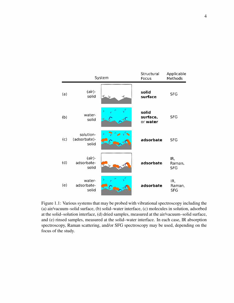
Fig. 1.1 shows various interfacial environments. Scenarios such as the surface

of interest is sandwiched between two condensed phases is often seen in biological

environment. One of the difficulty is to achieve selectivity for the interfacial chemical

species (e.g. adsorbate on a surface), ignoring signals coming from the adjacent condensed

phases. In Fig. 1.1a, the signals coming from the bulk should be separated from the the

signals coming from the solid surface. Fig. 1.1b illustrates Fig. 1.1a being placed in water.

One may want to study the structural change of the solid surface or how water molecules

orient and stack near the solid surface. Last but not least, Fig. 1.1c represents another

scenario where selectivity for the interfacial chemical species is crucial.

I only want the vibrational signal from the adsorbate. The vibrational signal coming

from the same molecules floating in the solution should be excluded. In the three cases

mentioned above, techniques based on even orders of the electronic susceptibility tensor are

suitable since they do not produce spectral response from centro-symmetric environments.

In another words, molecules that are not ordered in a polar manner will not trigger a signal.

Therefore, techniques such as electronic second-harmonic generation [16–21], vibrational

sum-frequency generation (SFG) [22, 23, 23–29] and difference-frequency generation

(DFG) [30, 31] are ideal for probing interfacial structures. Although in some scenarios a

χ(2) based spectroscopy technique such as SFG is an obvious choice to achieve interfacial

specificity, IR and Ramman scattering may also be considered in situations where the

surface is dried after adsorption from solution (Fig. 1.1d) or the solution is washed away

and replaced with water (Fig. 1.1e). By leveraging polarized light, IR [32–36], Raman

[37–43], SHG [44–49], SFG [22, 50–59] have become techniques capable of determining

quantitative structural information.

Extracting quantitative structural information involves creating a model spectra that

3

matches the experimental spectrum. Dipole moment and polarizability of a molecule

produces the spectrum signals. They are dependent on the conformation of the molecule.

That is, if the conformation of a molecule changes, the molecule’s dipole moment and

polarizability change as well. It is obvious that the number of possible dipole moments

and polarizability would be enormous for a big molecule. Besides that, there are also Euler

angles (tilt, twist and azimuthal) that play direct part in dictating the spectroscopy response.

In this study, I limit the number of possible dipole moment and polarizability by studying

small but crucial molecules, amino acids. I also limit the Euler angle parameter space by

considering only tilt and twist and assume isotropy in the azimuthal angular distribution.

Even with all the limitations, the number of candidate spectra is still great and the possible

combination of them is even greater. Trying to build the model spectrum from a large

number of candidate spectra to match the experimental spectrum would take a lot of time

and computational resources. A new algorithm is in need for building a model spectrum to

match the experimental one from the candidates.

Linear programming is a very promising approach to such problem. It is a method to

achieve an optimal solution (maximum or minimum) whose requirements are represented

in linear equality/inequality. In world war II, linear programming was used to plan military

activities to reduce costs and increase enemy’s losses [60]. In this case, I want to find

the best combination of the candidate spectrum that matches the experimental spectrum.

With the right combination, I would have a modeled spectrum whose difference with the

experimental spectrum is minimum. Linear programming problem can be solved in pseudo

polynomial time [61]. It is still an open question as to whether linear programming admit

a strongly polynomial-time algorithm. Even so, by formulating the spectrum modeling

problem as linear programming, I can explore larger parameter space and avoid exponential

running time. Since this thesis is about extracting orientation information from the

vibrational spectra, the rest of this section is going to give introduction to vibrational spectra

techniques (IR, Raman and SFG) and their formalism.

4

Figure 1.1: Various systems that may be probed with vibrational spectroscopy including the(a) air/vacuum–solid surface, (b) solid–water interface, (c) molecules in solution, adsorbedat the solid–solution interface, (d) dried samples, measured at the air/vacuum–solid surface,and (e) rinsed samples, measured at the solid–water interface. In each case, IR absorptionspectroscopy, Raman scattering, and/or SFG spectroscopy may be used, depending on thefocus of the study.

5

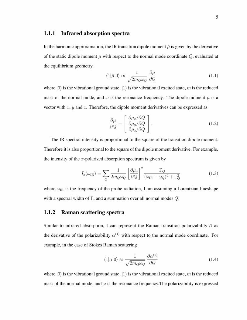
1.1.1 Infrared absorption spectra

In the harmonic approximation, the IR transition dipole moment µ is given by the derivative

of the static dipole moment µ with respect to the normal mode coordinate Q, evaluated at

the equilibrium geometry.

〈1|µ|0〉 ≈ 1√2mQωQ

∂µ

∂Q(1.1)

where |0〉 is the vibrational ground state, |1〉 is the vibrational excited state,m is the reduced

mass of the normal mode, and ω is the resonance frequency. The dipole moment µ is a

vector with x, y and z. Therefore, the dipole moment derivatives can be expressed as

∂µ

∂Q=

∂µx/∂Q∂µy/∂Q∂µz/∂Q

. (1.2)

The IR spectral intensity is proportional to the square of the transition dipole moment.

Therefore it is also proportional to the square of the dipole moment derivative. For example,

the intensity of the x-polarized absorption spectrum is given by

Ix(ωIR) =∑Q

1

2mQωQ

[∂µx∂Q

]2ΓQ

(ωIR − ωQ)2 + Γ2Q

(1.3)

where ωIR is the frequency of the probe radiation, I am assuming a Lorentzian lineshape

with a spectral width of Γ, and a summation over all normal modes Q.

1.1.2 Raman scattering spectra

Similar to infrared absorption, I can represent the Raman transition polarizability α as

the derivative of the polarizability α(1) with respect to the normal mode coordinate. For

example, in the case of Stokes Raman scattering

〈1|α|0〉 ≈ 1√2mQωQ

∂α(1)

∂Q(1.4)


mass of the normal mode, and ω is the resonance frequency.The polarizability is expressed

6

as a matrix, as it couples (x, y, z) components of the driving field with (x, y, z) components

of the induced dipole. The derivatives are therefore written as

∂α(1)

∂Q=

∂α(1)xx /∂Q ∂α

(1)xy /∂Q ∂α

(1)xz /∂Q

∂α(1)yx /∂Q ∂α

(1)yy /∂Q ∂α

(1)yz /∂Q

∂α(1)zx /∂Q ∂α

(1)zy /∂Q ∂α

(1)zz /∂Q

. (1.5)

The intensity of the Raman scattering is proportional to the square of the transition

polarizability which also means it’s proportional to the square of the polarizability

derivative. For example, with the incident field linearly-polarized along x, the x component

of the scattered radiation is given by

Ixx(ωIR) =∑Q

1

2mQωQ

[∂α

(1)xx

∂Q

]2ΓQ


. (1.6)

where ωIR is the frequency of the probe radiation, I am assuming a Lorentzian lineshape

with a spectral width of Γ, and a summation over all normal modes Q.

1.1.3 Vibrational sum-frequency spectra

Vibrational sum-frequency generation (SFG) spectroscopy has proven itself to be a useful

probe of molecules in non-centrosymmetric environments such as at surfaces and buried

interfaces. It is something that infrared absorption spectra and Raman scattering spectra

not capable of. The intensity is proportional to the squared magnitude of the second-order

susceptibility, |χ(2)|2. χ(2) itself is derived from the ensemble average of each molecule’s

second-order polarizability, α(2).

When only the infrared beam is near a molecular resonance α(2) is given by the

polarizablity derivative and dipole moment derivative product.

〈0|α|1〉〈1|µ|0〉 ≈ 1

2mQωQ

(∂α(1)

∂Q⊗ ∂µ

∂Q

). (1.7)

In other words, any of the 27 elements of α(2) may be evaluated from

α(2)lmn ≈

∂α(1)lm

∂Q

∂µn∂Q

. (1.8)

7

The spectral response is represented by the following complex-valued expression.

χ(2)xzx =

N

ε0

∑Q

1

2mQωQ

α(2)xzx

ωQ − ωIR − iΓQ(1.9)

in the case of an x-polarized infrared pump beam, z-polarized visible pump beam, and

x-polarized SFG emission. Here N is the number of molecules contributing to the SFG

process, ε0 is the vacuum permittivity, and i =√−1.

1.2 Aims and Scope

Linear programming is a type of optimization technique that can deal with large scale

decision problems of complexity. Simplex algorithm, which is a widely adapted to solve

linear program efficiently, is considered one of the greatest algorithm invented in the

20th century [62]. There exists algorithms that can solve linear programming problem in

weakly polynomial time, such as ellipsoid methods [63] and interior-point techniques [64].

However, whether or not there is a strong polynomial time algorithm to solve general

linear programming problem is still one of the biggest unanswered question [65]. Despite

linear programming’s great potential to solve decision problem efficiently, it had not been

intensively discussed and studied until after 1947. Fourier had published a paper that

solves the linear programming in 1837, but not much study follows up after that [60].

The thesis is not about linear programming itself, but rather how to use it to extract

quantitative orientation information from vibrational spectra. That is, how to formulate a

linear programming. In chapter 4, I gave a introduction to linear programming as to what is

it and why it is relevant. Along with detailed description in a step by step manner including

formalism to how to formulate a linear programming problem. However, it is extremely

important to create quality spectra candidates. Without them, the results returned by linear

programming would still be meaningless. Therefore, two chapters are devoted to discuss

the different aspects of generating vibrational spectra.

The rotation from one Cartesian coordinate system to another has been a well-

8

developed method [66–68]. However, in practice, the process is often very confusing

because the rotation operator expression changes drastically as the convention system

changes. To make things worse, identifying which convention system is used in a

particular formula is not straight forward. In section 2.2, I revisit the topic of coordinate

transformation and show how to do coordinate transformation without confusion. By

applying the knowledge from section 2.2, I demonstrate how to project dipole moment and

polarizability derivatives from molecular frame to laboratory frame with clearly described

convention and formalism in section 2.3. Section 2.4 discussed two approaches to deriving

orientation distribution for generating simulated spectrum.

There have been many studies discussing surface specificity of SHG/SFG [15, 22, 23,

49, 69, 70]. However, there is little for IR and Raman. In chapter 3, I compare the ability

of IR, Raman and SFG to detecting molecular orientation changes. First, I establish

the formalism of generating the spectroscopy responses for each techniques subject to

orientation distribution. Secondly, I present results considering gaussian distribution of

methyl tilt angles on a surface with common methyl symmetric vibrational mode. Next I

present results of leucine’s entire aliphatic C-H stretching mode when leucine is absorbed

onto a surface. Lastly, I investigate the scenario where I sample the molecular tilt and

twist angle distribution from molecular dynamic simulations instead of using analytical

distribution function such as gaussian distribution function.

9

Chapter 2

Methods

2.1 Vibrational Spectrum simulation overview

Atoms can be considered the building blocks for bigger molecules. All atoms are comprised

of protons, neutrons and electrons. Most of an atom’s mass is centered at the atom space,

taking up only a tiny portion of the total atom space. The rest of the space is taken up by

electrons. Although electrons are much, much lighter than protons and neutrons, they play

a very important role in chemical reaction. Atoms bind to one another stably by losing

or gaining electrons, forming molecules. Electronic structure is the state of motion of the

electrons. Electrons are not stationary like the nuclei of an atom. They are constantly

moving. Therefore, at different times, a molecule has different electronic structures and

different energies associated with each structure. The fact that the electrons are constantly

mobile means that the electron density in the molecule is uneven, which in turn, causes the

molecule to have electronic polarity. This phenomenon can be described mathematically

by

µ = α× E0 (2.1)

The expanded form µxµyµz

=

αxx αxy αxzαyx αyy αyzαzx αzy αzz

× ExEyEz

(2.2)

10

µ is a quantity called dipole moment, which is the electronic polarity of the molecule at a

given state. The dipole moment is induced when there is uneven distribution of electronic

cloud in the molecule. It is a product of α and E. α is a quantity called polarizability,

which describes the molecule’s ability to be polarized in an electromagnetic field. E

is the electromagnetic field in which the molecule resides. In the world of vibrational

spectroscopy, dipole moment and polarizability are very important in that their derivatives

gives signals to vibrational spectroscopic techniques such as IR, Raman and SFG.

A very important intermediate step is to come up with dipole moment derivatives and

polarizability derivatives. IR is essentially governed by sum of dipole moment derivatives

squared. Raman is essentially governed by sum of polarizability squared and SFG is

essentially governed by the square of absolute value of dipole moment derivatives and

polarizability product. The following sections will explain in details the expressions of the

three spectrum techniques.

The approach to obtaining the derivatives goes like this. The program chosen to do

electronic structure calculation is GAMESS [71]. First, do an hessian calculation on the

molecule, then one will get equilibrium coordinates, all of the vibrational modes along

with their frequencies and displacements. Second, imagine taking 7 snapshots when

the molecule is vibrating in a specific mode. At each moment the dipole moment and

polarizability are different. The values are obtained by doing a force field calculation

for each moment. Interpolate the dipole moment and polarizability at those moment and

differentiate the corresponding function; one can therefore obtains the dipole moment

derivatives and polarizability derivatives. These values are crucial in simulating IR, Raman

and SFG spectrums as discussed before. A lot of content in this chapter is based on my

previously co-authored paper “Rotations, Projections, Direction Cosines, and Vibrational

Spectra” [72].

11

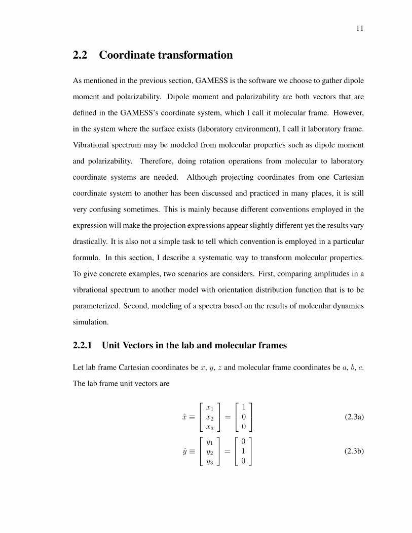
2.2 Coordinate transformation

As mentioned in the previous section, GAMESS is the software we choose to gather dipole

moment and polarizability. Dipole moment and polarizability are both vectors that are

defined in the GAMESS’s coordinate system, which I call it molecular frame. However,

in the system where the surface exists (laboratory environment), I call it laboratory frame.

Vibrational spectrum may be modeled from molecular properties such as dipole moment

and polarizability. Therefore, doing rotation operations from molecular to laboratory

coordinate systems are needed. Although projecting coordinates from one Cartesian

coordinate system to another has been discussed and practiced in many places, it is still

very confusing sometimes. This is mainly because different conventions employed in the

expression will make the projection expressions appear slightly different yet the results vary

drastically. It is also not a simple task to tell which convention is employed in a particular

formula. In this section, I describe a systematic way to transform molecular properties.

To give concrete examples, two scenarios are considers. First, comparing amplitudes in a

vibrational spectrum to another model with orientation distribution function that is to be

parameterized. Second, modeling of a spectra based on the results of molecular dynamics

simulation.

2.2.1 Unit Vectors in the lab and molecular frames

Let lab frame Cartesian coordinates be x, y, z and molecular frame coordinates be a, b, c.

The lab frame unit vectors are

x ≡

x1

x2

x3

=

100

(2.3a)

y ≡

y1

y2

y3

=

010

(2.3b)

12

Figure 2.1: Illustration of vectors that may be used to define the molecular-frame unitvectors for a water molecule. (a) In the case where both O–H bond lengths are known tobe fixed and equal, one can define ~c as the vector that runs from the midpoint M of thetwo H atoms to the O atom. ~a is then simply defined between the two H atoms. (b) In thecase where the bond lengths may be unequal, it may be simpler to define ~a first, betweenthe two H atoms. ~c would then originate from a point P along ~a, such that the vectordefined between P and the O atom is perpendicular to ~a. These decisions should followfrom whatever is most clear or logical for a particular molecule. In both cases, ~b may beobtained in the last step from the cross product relationship between the unit vectors in aright-handed coordinate system.

z ≡

z1

z2

z3

=

001

(2.3c)

If the molecule of interest is a linear shape, it would be very confusing if I choose

something other than the its long axis. Let’s call this long axis c; the tilt angle which brings

the z into c is θ. If the molecule is ”cigar-like”, then it doesn’t matter how you choose

your a and b molecular axis. As long as a, b and c are all perpendicular to one another and

follows the right-handed coordinate system form, which is defined as

a× b = c (2.4)

However, if the molecule of interest has a flat part, it is highly recommended to choose a

or b that lies in the plane of the flat region, as shown in 2.1.

Now that I have vectors ~a, ~b, ~c vectors in molecular frame, let’s turn them into unit

vectors a, b, c.

a =~a

‖~a‖(2.5a)

c =~c

‖~c‖(2.5b)

13

It’s easy to calculate the unit vector b from a and c. This is done by re-arranging Eq. 2.4.

b = c× a (2.5c)

Since a and c are unit vectors, the cross product of a and c is also a unit vector. So there is

no need to normalize ~b. The order of the cross product is extremely important. c × a = b

and a × c = −b; the former is a right-handed coordinate system and the latter one is a

left-handed coordinate system. I now have the molecular frame unit vectors.

a ≡

a1

a2

a3

(2.6a)

b ≡

b1

b2

b3

(2.6b)

c ≡

c1

c2

c3

(2.6c)

With Eq. 2.3, I have a complete set of unit vectors in both lab and molecular frame.

2.2.2 Direction cosine matrix

The direction cosine matrix (DCM) is a matrix that can be used to directly transform Eq. 2.3

into Eq. 2.6. In fact, all the vectoral properties can be transformed from coordinate system

represented by Eq. 2.3 (lab frame) to coordinate system represented by Eq. 2.6 (molecular

frame). The matrix gets its name because each element is a cosine between vector i in the

lab frame and vector l in the molecular frame.

D =

cos ξxa cos ξxb cos ξxccos ξya cos ξyb cos ξyccos ξza cos ξzb cos ξzc

(2.7)

I can view the matrix in a different way. Take the top left D1,1 as an example.

cos ξxa =x · a‖x‖‖a‖

=x1a1 + x2a2 + x3a3

1 · 1= a1

(2.8)

14

Because x1 is one and x2 and x3 are zero, the only surviving term is a1. Repeating the

same process for all of the elements in the matrix, the final DCM may be written in a very

compact form

D =

a1 b1 c1

a2 b2 c2

a3 b3 c3

. (2.9)

The inverse of the DCM is also very important, as it takes the vectoral properties from

molecular frame into lab frame. Since the DCM is an orthogonal matrix, its inverse is also

its transpose

D−1 =

a1 a2 a3

b1 b2 b3

c1 c2 c3

= DT . (2.10)

As one can tell, D and D−1 are very similar. It is important not to confuse one with the

other. Bear in mind that the D provides tranformation from lab frame to molecular frame.

D ·

100

=

a1

a2

a3

and D−1 provides tranformation from molecular frame to lab frame.

D−1 ·

a1

a2

a3

=

100

With these two equations, one can quickly do a sanity test on the correctness of rotation

and identify DCM and inverse DCM.

2.2.3 Obtaining the Euler angles

The Euler angles is a popular definition and convention for paramerizing rotations. It is

by no means, the only choice. But Euler angles do permit nice visualization in three

dimensions. In the previous section, I construct the form of DCM. It so happens that I

can extract the Euler angles from the DCM. I have already defined θ as the tilt angle, it

is the angle between z and c. There are two more angles φ and ψ. φ is the azimuthal

angle of rotation about z. To be more precise, it is the angle between x and the projection

of a into the xy-plane. ψ is the twist angle about c. The definitions of these angles are

15

Figure 2.2: The Euler angles represented as the spherical polar angles θ, φ and ψ. [66]

Figure 2.3: Illustration of the 3 successive rotations that transform the lab (x, y, z)coordinate system into the molecular (a, b, c) frame. In the case of an intrinsic set ofrotations (top row), one performs Rz(φ) a rotation by φ about z, Ry′(θ) rotation by θabout y′, and finally Rc(ψ) rotation by ψ about c. In the case of an extrinsic set of rotations(bottom row), one performs Rz(ψ) a rotation by ψ about z, Ry(θ) rotation by θ about y,and finally Rz(φ) rotation by φ about z. [66]

illustrated in Fig. 2.2. Technically speaking, both φ and ψ are both azimuthal angles about

different vectors. To avoid confusion, I refer only φ as azimuth and ψ as twist angle. Three

successive rotations can turn molecular frame into lab frame, as illustrated in Fig. 2.3 The

first operation is a rotation by about the molecular c axis, followed by a rotation about

N , the line of nodes that is defined by the current location of the molecular b axis (see

Fig. 2.3b). Finally a rotation is performed about the lab frame z axis. This follows the right-

handed convention, rotating counter-clockwise when looking towards the origin. There are

two conventions for describing and applying the rotation operators: intrinsic and extrinsic.

16

Intrinsic rotations are applied to a rotating coordinate system, where subsequent rotations

are performed on axes that exist only as a result of a prior rotation operation. On the other

hand, extrinsic rotations are applied about a fixed frame. In other words, the successive

rotation operators are always about x-, y-, or z-axes, even in intermediate step. Extrinsic

rotations can be easily described by the three following operators

Rz(ψ) =

cosψ − sinψ 0sinψ cosψ 0

0 0 1

(2.11a)

Ry(θ) =

cos θ 0 sin θ0 1 0

− sin θ 0 cos θ

(2.11b)

Rz(φ) =

cosφ − sinφ 0sinφ cosφ 0

0 0 1

(2.11c)

These operators represent rotating about a fixed frames’ Z, Y, Z axis for ψ, θ and φ

respectively. Having seen the Fig. 2.3, one may think the rotation from molecular frame to

lab frame is the product of the three extrinsic operators in the order they are listed. This is a

common misunderstanding. The rotations illustrated in Fig. 2.3 are not extrinsic rotations.

Extrinsic rotations applied to fixed frames. The rotations shown in Fig. 2.3 are performed

on axis that is the result of the previous rotation. Luckily, there is a straightforward

relationship between extrinsic and intrinsic rotations. Any extrinsic rotation is equivalent

to an intrinsic rotation by the same angles but with inverted order of elemental rotations,

and vice-versa. Therefore, the intrinsic rotations illustrated in Fig. 2.3 can be described by

extrinsic operator as

D(θ, φ, ψ) = Rz(φ) ·Ry(θ) ·Rz(ψ)

=

cosφ cos θ cosψ − sinφ sinψ − cosφ cos θ sinψ − sinφ cos θ sin θ cosφsinφ cos θ cosψ + cosφ sinψ − sinφ cos θ sinψ + cosφ cosψ sin θ sinφ

− cosψ sin θ sinψ sin θ cos θ

.(2.12)

17

D is a function of the Euler angles, for brevity I will write only D instead of D(θ, φ, ψ).

Looking closely at Eq. 2.12 The Euler angles may be obtained from

θ = cos−1D3,3 (2.13a)

φ = tan−1 D2,3

D1,3

(2.13b)

ψ = tan−1 D3,2

−D3,1

. (2.13c)

Note that quadrant preservation is tricky in the arctangent evaluation as both φ and ψ

are defined in the interval (−π, π). For example, arctan(1/1) is π/4 rad or 45. arctan(-1/-1)

will also be evaluated to π/4 rad or 45 as well where it clearly should be 3π/4 rad, or 135.

To prevent this from happening, arctan2 function is devised to prevserve the quadrant by

considering the signs of both vector components.

2.3 Projecting molecular properties into the lab frame

Here I deal with the situation where an optical property is known (possibly through an

electronic structure calculation) in the (a, b, c) molecular frame defined by the electronic

structure calculation program (GAMESS). I wish to construct spectra based on snapshots

of a molecular dynamics simulation, where the coordinates of the molecule are given in the

laboratory frame.

2.3.1 Infrared absorption spectra

In the harmonic approximation, the IR transition dipole moment µ is governed by the

derivative of the dipole moment µ evaluated at the equilibrium geometry.

〈1|µ|0〉 ≈ 1√2mQωQ

∂µ

∂Q(2.14)


mass of the normal mode, and ω is the resonance frequency. The dipole moment is a

18

vectoral quantity (tensor of rank 1) with a, b and c components in the Cartesian molecular

frame, and so the derivative becomes

∂µ

∂Q=

∂µa/∂Q∂µb/∂Q∂µc/∂Q

. (2.15)

As the intensity of the IR absorption is proportional to the square of the dipole moment,

I wish to compute elements of (∂µ/∂Q)2 in the lab (i, j, k) frame. The requires

transformation as in∂µ

∂Q(θ, φ, ψ)

∣∣∣∣ijk

= D · ∂µ∂Q

∣∣∣∣lmn

(2.16)

Here I can see that ∂µ/∂Q in the lab frame is a function the Euler angles. This is equivalent

to writing∂µi∂Q

(θ, φ, ψ) =abc∑l

Dil∂µl∂Q

. (2.17)

2.3.2 Raman scattering spectra

Based on the formalism developed in the above section, I can consider that the Raman

transition polarizability α may approximated as the derivative of tge polarizability α(1)

with respect to the normal mode coordinate [67]. For example, in the case of Stokes Raman

scattering

〈1|µ|v〉〈v|µ|0〉 ≡ 〈1|α|0〉 ≈ 1√2mQωQ

∂α(1)

∂Q(2.18)

where the ground and first excited vibrational states are connected through the virtual

electronic state |v〉. The polarizability can be expressed as a matrix.

∂α(1)

∂Q=

∂α(1)aa /∂Q ∂α

(1)ab /∂Q ∂α

(1)ac /∂Q

∂α(1)ba /∂Q ∂α

(1)bb /∂Q ∂α

(1)bc /∂Q

∂α(1)ca /∂Q ∂α

(1)cb /∂Q ∂α

(1)cc /∂Q

. (2.19)

The intensity of the Raman scattering is proportional to the square of the lab frame

polarizability derivative. For example, with the incident field linearly-polarized along x,

19

the x component of the scattered radiation is given by

Ixx(ωIR) =∑Q

1

2mQωQ

[∂α

(1)xx

∂Q

]2ΓQ


. (2.20)

To project α(1) into the lab frame on an element-by-element basis

∂α(1)ij

∂Q(θ, φ, ψ) =

abc∑l

abc∑m

Dil Djm∂α

(1)lm

∂Q. (2.21)

There are 9 terms in the above expression, as each of α(1)aa , α(1)

ab , all the way to α(1)cc

contribute to α(1)xx . A similar expression then provides the 9 terms required to calculate

α(1)xy , and so on. 81 terms must be evaluated to complete α(1) in the lab frame. There is a

more efficient and straightforward way to do this.

∂α(1)

∂Q(θ, φ, ψ)

∣∣∣∣ijk

= D · ∂α(1)

∂Q

∣∣∣∣lmn

·D−1 (2.22)

As a result, transforming ∂α(1)/∂Q from molecular frame into the lab frame requires only

the multiplication of 3 matrices.

2.3.3 Vibrational sum-frequency spectra

Vibrational sum-frequency generation (SFG) spectroscopy has proven itself to be a useful

probe of molecules in non-centrosymmetric environments such as at surfaces and buried

interfaces. [23, 24, 28, 73–75] The intensity is proportional to the squared magnitude of

the second-order susceptibility, |χ(2)|2. χ(2) itself is derived from the ensemble average of

each molecule’s second-order polarizability, α(2). [74] in the case of an anti-Stokes Raman

transition from |1〉 to |0〉. When only the infrared beam is near a molecular resonance α(2)

is given by the tensor product

〈0|α|1〉〈1|µ|0〉 ≈ 1

2mQωQ

(∂α(1)

∂Q⊗ ∂µ

∂Q

). (2.23)

In other words, any of the 27 elements of the tensor α(2) may be evaluated from

α(2)lmn ≈

∂α(1)lm

∂Q

∂µn∂Q

. (2.24)

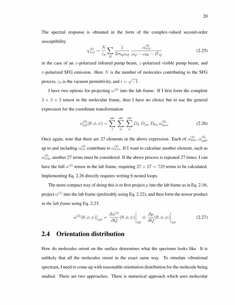
20

The spectral response is obtained in the form of the complex-valued second-order

susceptibility

χ(2)xzx =

N

ε0

∑Q

1

2mQωQ

α(2)xzx

ωQ − ωIR − iΓQ(2.25)

in the case of an x-polarized infrared pump beam, z-polarized visible pump beam, and

x-polarized SFG emission. Here N is the number of molecules contributing to the SFG

process, ε0 is the vacuum permittivity, and i =√−1.

I have two options for projecting α(2) into the lab frame. If I first form the complete

3 × 3 × 3 tensor in the molecular frame, then I have no choice but to use the general

expression for the coordinate transformation

α(2)ijk(θ, φ, ψ) =

abc∑l

abc∑m

abc∑n

Dil Djm Dkn α(2)lmn. (2.26)

Once again, note that there are 27 elements in the above expression. Each of α(2)aaa, α

(2)aab,

up to and including α(2)ccc contribute to α(2)

xxx. If I want to calculate another element, such as

α(2)xxy, another 27 terms must be considered. If the above process is repeated 27 times, I can

have the full α(2) tensor in the lab frame, requiring 27 × 27 = 729 terms to be calculated.

Implementing Eq. 2.26 directly requires writing 6 nested loops.

The more compact way of doing this is to first project µ into the lab frame as in Eq. 2.16,

project α(1) into the lab frame (preferably using Eq. 2.22), and then form the tensor product

in the lab frame using Eq. 2.23.

α(2)(θ, φ, ψ)∣∣ijk

=∂α(1)

∂Q(θ, φ, ψ)

∣∣∣∣ijk

⊗ ∂µ

∂Q(θ, φ, ψ)

∣∣∣∣ijk

(2.27)

2.4 Orientation distribution

How do molecules orient on the surface determines what the spectrum looks like. It is

unlikely that all the molecules orient in the exact same way. To simulate vibrational

spectrum, I need to come up with reasonable orientation distribution for the molecule being

studied. There are two approaches. There is numerical approach which uses molecular

21

dynamic simulation and analytic method which follows specific distribution function, in

this case, Gaussian distribution.

2.4.1 Numerical method - Molecular Dynamic (MD) Simulation

MD simulation is one way to find out the populations of different orientation, which is

essential for generating vibrational spectra. The benefit of this is that it adds flexibility and

is not constrained to specific functional form. However, it is much more time consuming. A

few seconds worth of MD simulation could take days or months to generate depending on

the size of the molecule and the complexity of the environment. Another way is to assume

the population of different orientation follows a specific distribution function. Gaussian

distribution is a good example and will be discussed in more detail in the next section.

The program that is chosen to perform molecular dynamic simulation is GROMACS.

By specifying system such as the molecule of interest, solution type and surface type,

GROMACS simulates the physical movement of molecules in the system with Newtonian

physics. The GROMACS output file is a series of frames. Each frame is a snapshot of

the system at a particular time. The location and orientation of a particular molecule is

represented by the Cartesian coordinates of each atoms in the molecule. Since I am only

interested in molecules on the surface, only frames with molecules close to the surface is

selected to study. The information to extract from the frames are how the molecules orient

on the surface (Euler angles) in the form of orientation distribution. Keep in mind that the

electronic structure calculation is done in one coordinate system (molecular frame) and the

MD simulation is done in yet another coordinate system (laboratory frame). To properly

generate predicted vibrational spectra based on the orientation distribution obtained from

MD simulation, I need to project the vectoral values in molecular frame such as dipole

moment and polarizability into laboratory frame.

22

2.4.2 Analytic method - Gaussian Distribution

This is a counterpart of the MD simulation. With MD, I go through each frame to obtain

the orientation distribution. Here, it is assumed that the molecule orientation distribution

follows Gaussian distribution. If only θ is being considered, then the distribution function

can be expressed as Eq. 2.28.

f(θ) = exp

[−(θ − θ0)2

2σ2

](2.28)

The θ0 dictates the mean orientation population and the σ dictates deviation from the

mean orientation population. The orientation distribution gathered from MD does not

necessarily resemble that of any distribution function. Simulating orientation distribution

with distribution function is faster. A numerical approach (molecular dynamic simulation)

requires considering every single frame to aggregate a final orientation distribution. Where

as in analytic approach (Gaussian distribution), orientation distribution can be derived

directly from a math expression.

23

Chapter 3

Sensitivity of different techniques toorientation distribution

3.1 Overview

In chapter 2, I have discussed some of the aspects of creating vibrational spectrum, such

as properties projection and how to obtain mock orientation distribution. In this chapter, I

am going to compare the orientation sensitivity of different spectroscopy techniques. This

is done by generating spectra for IR, Raman and SFG starting with a simple orientation

distribution of a single vibrational mode, leading up to a complex orientation distribution

with multiple vibrational modes and then comparing their spectra response sensitivity to

the features of the orientation distribution. The result of this chapter allows us to choose

appropriate spectroscopy technique for generating spectrum that is rich in orientation

information. This chapter is based on my previously co-authored paper “IR Absorption,

Raman Scattering, and IR-vis Sum-frequency Generation Spectroscopy as Quantitative

Probes of Surface Structure” [76].

3.2 Formalism and molecular response

3.2.1 Vibrational Response

The formalism for IR, Raman and SFG spectrum has been developed and shown in section

1.1. I will discuss it briefly here again. In the case of IR, the response intensity of x-

24

polarized absorption spectrum under harmonic approximation is governed by

Ix(ωIR) ∝ N∑q

1

2mqωq

⟨[∂µx∂Q

]2

q

⟩Γ2q

(ωIR − ωq)2 + Γ2q

(3.1)

Ix represents x-polarized intensity. The same expression applies to Iy and Iz. ωIR is the

frequency of the probe radiation. µ is the dipole moment. mq, ωq, Γq, Qq are the reduced

mass, resonance frequency, homogeneous linewidth, and normal mode coordinate of the

qth vibrational mode. x-polarized Raman spectrum has similar approximated expression

Ixx(∆ω) ∝ N∑q

1

2mqωq

⟨[∂α

(1)xx

∂Q

]2

q

⟩Γ2q

(∆ω − ωq)2 + Γ2q

(3.2)

where ∆ω is the Stokes Raman shift and α(1)xx is one of the 9-element polarizability tensor.

The last technique is visible-infrared sum-frequency generation (SFG). The response is

second-order susceptibility tensor χ(2). For instance, χ(2)xxx is probed in such way that

a x-polarized visible incoming beam at frequency ωvis and x-polarized infrared beam

incoming with frequency ωIR are incident to the sample, and the x-component of the SFG

at frequency ωSFG = ωvis + ωIR is selected for detection. When only the infrared beam is

close to a molecular resonance, the response intensity is governed by

χ(2)xxx(ωIR) =

N

ε0

∑q

1

2mqωq

⟨[∂α

(1)xx

∂Q

]q

[∂µx∂Q

]q

⟩1

ωq − ωIR − iΓq(3.3)

As one can see, χ(2) is a complex value because of i =√−1 in the denominator. Therefore,

the real and imaginary components of the second-order susceptibility can be determined.

The SFG response can be shown as Im[χ(2)xxz(ωIR)].

3.2.2 Molecular orientation distribution

General description. All of the molecular properties such as dipole moments and

polarizability derivatives are defined in the molecular frame (x, y, z). However, they are

only valuable when they are put in the right context, which is the laboratory frame. The

transition involves projecting these values into the lab frame based on their Euler angles

25

(θ, φ, ψ) in the lab frame. These angles can be obtained through molecular dynamic

simulation (numerical approach) or orientation distribution function (analytic approach).

For example, if the coordinates of all the molecules are known, I can compute x-polarized

IR as

N

⟨[∂µx∂Q

]2⟩

=∑

molecules

[∂µx∂Q

(θ, φ, ψ)

]2

(3.4)

The projection into the lab frame dipole moment derivative can be expressed as

∂µx∂Q

(θ, φ, ψ) = D1,1(θ, φ, ψ)∂µa∂Q

+D1,2(θ, φ, ψ)∂µb∂Q

+D1,3(θ, φ, ψ)∂µc∂Q

(3.5)

where D is a 3x3 direction cosine matrix. Similar expressions exist for Raman and SFG,

although in more complex forms. In the case of analytic approach where an orientation

distribution is determined by an orientation distribution function instead of deriving from

individual coordinates, the dipole moment can be computed as

⟨[∂µx∂Q

]2⟩≈ Nc

∫Ω

f(Ω)

[∂µx∂Q

(Ω)

]2

∂Ω

≡

∫ 2π

0

∫ 2π

0

∫ π

0

f(θ, φ, ψ)

[∂µx∂Q

(θ, φ, ψ)

]2

sin θ ∂θ ∂φ ∂ψ∫ 2π

0

∫ 2π

0

∫ π

0

f(θ, φ, ψ) sin θ ∂θ ∂φ ∂ψ

(3.6)

Isotropic averages. In a bulk liquid phase, such as water. There is no preference in

orientation. All Euler angles are uniformly distributed. Therefore achieving isotropic

distribution. The spectral response in the environment is very different for IR, Raman

and SFG. For IR, all elements of the dipole moment derivative are equal and they represent

the average of the molecular frame dipole moment derivative.

⟨[∂µx∂Q

]2⟩

=

⟨[∂µy∂Q

]2⟩

=

⟨[∂µz∂Q

]2⟩

=1

3

([∂µa∂Q

]2

+

[∂µb∂Q

]2

+

[∂µc∂Q

]2)

(3.7)

26

In the case of Raman scattering, all 3 values 〈[∂α

(1)ij /∂Q

]2

〉 with i = j are equivalent,

as are the 6 values for which i 6= j. As a result, any two elements of these sets may be used

to calculate the Raman depolarization ratio in solution [72]. Sum-frequency generation

requires a net polar orientation to break inversion symmetry. The technique is valued for

its surface specificity as all 21 achiral elements of χ(2)ijk (excluding the 6 elements for which

i 6= j 6= k) have an isotropic average of zero.

Uniaxial tilt and twist distributions. In most cases, I assume isotropy distribution in

the azimuthal angle φ since it is the most common scenario. This may not be true on the

surfaces that are rubbed or striped causing alignment in the plane of the surface. Other than

that, symmetry may only break in the up-down direction. If I assume isotropic orientation

distribution in both φ and ψ and consider tilt angle θ follows Gaussian distribution. The

resulting orientation distribution function would be

f(θ) = Nc exp

[−(θ − θ0)2

2σ2

](3.8)

Gaussian distribution looks like a bell curve. In this context, θ0 is the center of the bell-

curve (mean tilt angle). σ is the half-width of the bell curve. Nc is a normalization constant.

Taking the x- polarized IR absorption spectrum as an example, the response is calculated

according to Eq. 3.6. When the half-width σ is small, the bell curve will look like a tall thin

peak. If the width is infinitesimal δ(θ−θ0), I end up with the 〈[∂µx/∂Q]2〉 = 〈[∂µy/∂Q]2〉.

That is, identical x- and y- polarized IR absorption spectra. For Raman spectra, I am still

considering scenarios where far from electronic resonance, Raman tensor being symmetric.

Therefore, I still have 〈[∂α(1)ij /∂Q]2〉 = 〈[∂α(1)

ji /∂Q]2〉. However, I now have four unique

elements instead of two in the isotropic case. They are

27

⟨[∂α

(1)xx

∂Q

]2⟩=

⟨[∂α

(1)yy

∂Q

]2⟩(3.9a)⟨[

∂α(1)xy

∂Q

]2⟩=

⟨[∂α

(1)yx

∂Q

]2⟩(3.9b)⟨[

∂α(1)xz

∂Q

]2⟩=

⟨[∂α

(1)yz

∂Q

]2⟩=

⟨[∂α

(1)zx

∂Q

]2⟩=

⟨[∂α

(1)zy

∂Q

]2⟩(3.9c)⟨[

∂α(1)zz

∂Q

]2⟩. (3.9d)

For simplicity, I write these Raman responses as xx = yy, xy = yx, xy = xz = zx = zy,

and zz. I refer to each unique response by the first member of each set. In SFG spectra, 7

out of 27 elements of χ(2) are now non-zero and 3 out of 7 are unique.

〈α(2)xxz〉 = 〈α(2)

yyz〉 (3.10a)

〈α(2)xzx〉 = 〈α(2)

yzy〉 = 〈α(2)zxx〉 = 〈α(2)

zyy〉 (3.10b)

〈α(2)zzz〉 (3.10c)

Again, for simplicity, I write xxz = yyz, xzx = yzy = zxx = zyy, and zzz. The

amplitudes and imaginary part of the spectra associated with these four unique elements

are labeled according to the first member of each set.

3.3 Results and discussion

3.3.1 Vibrational modes dominated by a single element in the IR andRaman response

I now consider a vibrational mode dominated by a single element of the dipole moment

∂µ

∂Q=

00

∂µc/∂Q

(3.11)

28

and a single element of the polarizability derivative

∂α(1)

∂Q=

0 0 00 0 0

0 0 ∂α(1)cc /∂Q

. (3.12)

Both of these properties are along the bond axis. That is why I call this case uniaxial case.

This describes a carbonyl group or a single C–H bond. The intensity of the IR absorption

spectra are proportional to the square of the laboratory frame dipole moment derivative as

described in Eq. 3.1. In this particular case, the resulting expressions are⟨(∂µx∂Q

)2⟩

=1

2

(∂µc∂Q

)2 [1− 〈cos2 θ〉

](3.13a)⟨(

∂µz∂Q

)2⟩

=

(∂µc∂Q

)2

〈cos2 θ〉, (3.13b)

and the Raman scattering may bear the form⟨(∂α

(1)xx

∂Q

)2⟩=

3

8

(∂α

(1)cc

∂Q

)2 [1− 2〈cos2 θ〉+ 〈cos4 θ〉

](3.14a)⟨(

∂α(1)xy

∂Q

)2⟩=

1

8

(∂α

(1)cc

∂Q

)2 [1− 2〈cos2 θ〉+ 〈cos4 θ〉

](3.14b)⟨(

∂α(1)xz

∂Q

)2⟩=

1

2

(∂α

(1)cc

∂Q

)2 [〈cos2 θ〉 − 〈cos4 θ〉

](3.14c)⟨(

∂α(1)zz

∂Q

)2⟩=

(∂α

(1)cc

∂Q

)2

〈cos4 θ〉. (3.14d)

In the uniaxial case, the expression for lab frame hyperpolarizability which dictates the

SFG response intensity is also very compact.

〈α(2)xxz〉 = 〈α(2)

xzx〉 =1

2α(2)ccc

(〈cos θ〉 − 〈cos3 θ〉

)(3.15a)

〈α(2)zzz〉 = α(2)

ccc〈cos3 θ〉. (3.15b)

There are now only two unique elements of the hyperpolarizability (and therefore χ(2))

in the lab frame. These elements of α(2) directly influenced the measured SFG intensities

according to the polarization (s or p) of the incoming visible and IR beams, and the (s or

29

Figure 3.1: The x and z components of the IR absorption (first row), xx, xy, xz, and zzcomponents of the Raman scattering (middle row), and xxz, xzx, and zzz components ofthe hyperpolarizability (bottom row) for a uniaxial vibrational mode as a function of themean tilt angle θ0 and half-width σ of a Gaussian distribution of the methylC3 axes. Darkerred colors indicate higher intensity. Horizontal dashed white lines at σ = 7.5 and σ = 50

indicate distribution widths for which derivatives are displayed in Fig. 3.2.

30

p) generated SFG beam. As stated in our description of the experiments, 〈α(2)xxz〉 is probed

with Issp, while 〈α(2)zzz〉 is one of four contributions to Ippp.

I can verify the predicted response when the narrow distributions (σ is almost zero,

along the bottom edge of the subplots) since the trigonometric functions in Eq. 3.13 and

Eq. 3.15 are relatively simple. For instance, the z- polarized component is proportional to

cos2 θ. This means the highest intensity happens when the methyl group is perpendicular

to the surface. The x- polarized IR has the highest intensity when θ = 90 because it is

proportional to 1 − cos2 θ (or sin2 θ). Same analogy applies to xy Raman component and

xyz SFG component. At narrow distribution, the maxima happens at θ other than 0 or 90.

Fig. 3.1 directly plotted the variation in signal intensity as the θ0 and σ of the normal

distribution varies. However, it is not intuitive to compare the orientation sensitivity of the

three technique this way. It is difficult in that it is the combination of the magnitude of the

signal intensity and the amount in which the signal varies that defines the sensitivity. In

other words, the one which has the biggest difference in magnitude does not necessary

mean it is the most sensitive. It is the percentage change that shows the sensitivity.

Therefore, I normalized the signals within each techniques and calculated the derivatives

with respect to θ0. Two scenarios are shown in Fig. 3.2. (a–c) show a narrow distribution

with σ = 7.5 and (d–f) show a wide distribution with σ = 50.

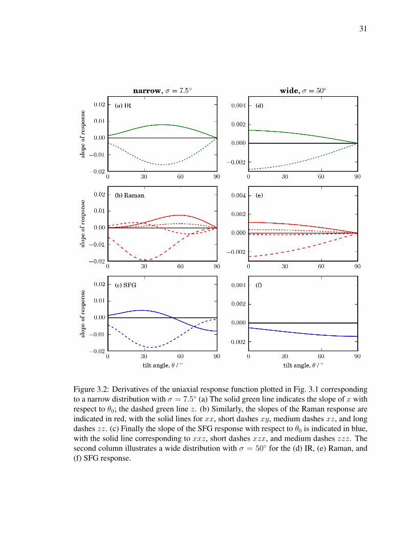
Looking at Fig. 3.2, especially the lines that represent IR z, Raman zz and SFG zzz

curves, one can observe that Raman has the steepest slope, followed by SFG and then

IR.The steepness of the slope correspond to the sensitivity since the percentage change is

higher. Looking at the x- polarized response, Raman is once again more sensitive than

IR. (Cannot compare to SFG since χ(2)xxx = 0). Comparing the rest of the elements are

much more difficult since they all show comparable sensitivity to θ. However, the bottom

line is, in scenarios such as narrow orientation distribution, Raman has higher sensitivity to

orientational changes.

31

Figure 3.2: Derivatives of the uniaxial response function plotted in Fig. 3.1 correspondingto a narrow distribution with σ = 7.5 (a) The solid green line indicates the slope of x withrespect to θ0; the dashed green line z. (b) Similarly, the slopes of the Raman response areindicated in red, with the solid lines for xx, short dashes xy, medium dashes xz, and longdashes zz. (c) Finally the slope of the SFG response with respect to θ0 is indicated in blue,with the solid line corresponding to xxz, short dashes xzx, and medium dashes zzz. Thesecond column illustrates a wide distribution with σ = 50 for the (d) IR, (e) Raman, and(f) SFG response.

32

3.3.2 Methyl group response

The discussion in the previous section has allowed us to make comparisons between the

three techniques in terms of orientaional sensitivity. There is a simple relationship between

the tilt angle and single element of IR and Raman response along the bond axis. However,

since the results are sensitive to nature of the specific vibrational mode, I should also

consider a more complex mode, such as the methyl symmetric stretch. The dipole moment

derivative of the common C3v symmetry functional group is governed by

∂µ

∂Q=

00

∂µc/∂Q

=

00−1

(3.16)

and the expression for polarizability is

∂α(1)

∂Q=

∂α(1)aa /∂Q 0 0

0 ∂α(1)aa /∂Q 0

0 0 ∂α(1)cc /∂Q

=

2.5 0 00 2.5 00 0 −1

(3.17)

where the molecular c axis is aligned with the methyl C3 axis, pointing from the

carbon atom towards the hydrogen atoms. Here I can see that, although the dipole moment

derivative is still assumed to lie entirely along the three-fold symmetry axis, I now introduce

an additional non-zero element of the polarizability derivative perpendicular to this axis.

Furthermore, methyl represents a significant departure from the Raman tensor dominated

by ∂α(1)cc /∂Q as ∂α(1)

aa /∂Q is larger than this element by a factor of 2.5. The resulting

expressions for the lab-frame IR response are therefore identical to those presented in

Eq. 3.14, but the Raman expressions become

33

Figure 3.3: Illustration of (a) a methyl group with the molecular c vector passing throughits C3 axis. θ is the angle between the surface normal z and the c vector; the twist angleψ is assumed to be uniformly distributed. (b) In the case of a non-uniaxial entity definingthe ac-plane, the tilt and twist angles are both relevant. (c) The leucine molecule-fixedcoordinates as the (a, b, c) unit vectors. The c axis passes from the γ carbon atom (CG) tothe α carbon atom (CA). a passes from the β carbon atom to the line joining CG and CB;b is obtained by vector cross product of a and c. Here I also consider the twist ψ about thec axis.

⟨(∂α

(1)xx

∂Q

)2⟩=

3

8

(∂α

(1)aa

∂Q

)2

+1

4

(∂α

(1)aa

∂Q

)(∂α

(1)cc

∂Q

)+

3

8

(∂α

(1)cc

∂Q

)2

(3.18a)

+1

4

(∂α(1)aa

∂Q

)2

+ 2

(∂α

(1)aa

∂Q

)(∂α

(1)cc

∂Q

)− 3

(∂α

(1)cc

∂Q

)2 〈cos2 θ〉

+3

8

[(∂α

(1)aa

∂Q

)−

(∂α

(1)cc

∂Q

)]2

〈cos4 θ〉⟨(∂α

(1)xy

∂Q

)2⟩=

1

8

[(∂α

(1)aa

∂Q

)−

(∂α

(1)cc

∂Q

)]2 [1− 2〈cos2 θ〉+ 〈cos4 θ〉

](3.18b)⟨(

∂α(1)xz

∂Q

)2⟩=

1

2

[(∂α

(1)aa

∂Q

)−

(∂α

(1)cc

∂Q

)]2 [〈cos2 θ〉 − 〈cos4 θ〉

](3.18c)

⟨(∂α

(1)zz

∂Q

)2⟩=

(∂α

(1)aa

∂Q

)2

+ 2

(∂α(1)aa

∂Q

)(∂α

(1)cc

∂Q

)−

(∂α

(1)aa

∂Q

)2 〈cos2 θ〉 (3.18d)

+

[(∂α

(1)aa

∂Q

)−

(∂α

(1)cc

∂Q

)]2

〈cos4 θ〉.

The non-zero elements of the hyperpolarizability still holds a simple form even though

34

more elements of the Raman tensor are added.

〈α(2)xxz〉 =

1

2

(α(2)aac + α(2)

ccc

)〈cos θ〉+

1

2

(α(2)aac − α(2)

ccc

)〈cos3 θ〉 (3.19a)

〈α(2)xzx〉 =

1

2

(α(2)ccc − α(2)

aac

) (〈cos θ〉 − 〈cos3 θ〉

)(3.19b)

〈α(2)zzz〉 = α(2)

aac〈cos θ〉+ (α(2)ccc − α(2)

aac)〈cos3 θ〉. (3.19c)

The first row, second row and bottom row represents IR, Raman and SFG respectively

as a function of θ0 and σ of the tilt Gaussian distribution described in Eq. 3.8. As described

in the previous, the x- and y- components of the IR intensity are the same when considering

isotropic azimuthal angle. Therefore, I only displayed x and z. The first thing I observe

is that when σ ≈ 90 (effectively isotropic distribution), x ≈ y. This is equivalent to

x = y = z = 1/3 and is expected according to Eq. 3.7. Moving on to the trends observed

at small σ, the IR intensity for x increases when θ0 increases whereas the IR intensity for z

decreases when θ0 increases. This makes sense since the methyl dipole moment is parallel

with the x- polarized and z- polarized IR probe when θ0 = 90 and θ0 = 0 respectively.

Another observation is that z has the highest intensity. This is due to the fact that, for

the orientation distribution I assume, all of the molecules could align along z (θ0 = 0,

σ ≈ 0), while having molecules uniformly distributed in the xy-plane when θ0 = 90. The

last observation is that the z-polarized component for IR adsorption at narrow distribution

is more sensitive than the x- and y- polarized component. For broad distribution, IR is

simply not very sensitive to the change in title angle.

Moving on to the results of Raman scattering shown in the middle row of Fig. 3.4.

In the case of narrow distributions, all of the elements in the Raman tensor are sensitive

to mean tilt angle and width of the tilt Gaussian distribution. Take xz for example, its

intensity increases as θ0 increases until approximately 45 but starts decreasing when the

methyl group is closing on to the plan of the surface. zz shares the same behavior with its

peak intensity at around θ0 = 25. The results also show that when the σ of the distribution

gets bigger (isotropic distribution), then xx = zz and xy = xz. These observations indicate

35

Figure 3.4: The x and z components of the IR absorption (first row), xx, xy, xz, and zzcomponents of the Raman scattering (middle row), and xxz, xzx, and zzz components ofthe hyperpolarizability (bottom row) for a methyl symmetric stretch as a function of themean tilt angle θ0 and half-width σ of a Gaussian distribution of the methyl C3 axes. Eightcombinations A–H of the parameters θ0 and σ in the Gaussian distribution are shown asannotations on the plots for comparison with Fig. 3.6 and Fig. 3.7. Positive values areshaded in red with solid contours; negative values are shaded in blue with dashed contours.Horizontal dashed white lines at σ = 7.5 and σ = 50 indicate distribution widths forwhich derivatives are displayed in Fig. 3.5.

36

that Raman may have shown more sensitivity to orientational change than IR at narrow

distribution.

Hyperpolarizability tensor α(2) intensity, which is the a measure of heterodyne SFG

spectroscopy response is shown in the bottom row of Fig. 3.4 as a result of varying θ0

and σ. Representing α(2)ijk, dashed contour and blue shading indicate negative value while

solid contour ad red shading indicate positive values. When σ is large (isotropic average),

the hyperpolarizability tensor α(2) becomes small. For this reason, SFG shows the most

contrast when θ0 and/or σ of the orientation distribution is very large or small. One

may also notice that, for relatively narrow distribution (σ < 20), xzx is more sensitive

to orientational changes (greater variation in intensity) than the xxz element. This is

consistent with the understanding in SFG spectroscopy that ssp polarization is not as

sensitive to symmetric modes as other polarization combination. Most noticeably, zzz

shows most sensitivity to orientation distribution change. This may be one reason that

the ppp element, which includes xxz, xzx, zxx and zzz, show very good sensitivity to

orientation change in some cases [47, 49].

The most direct way to compare these techniques in terms of orientation sensitivity is

the rate of changing (slopes) with respect to θ0. Two values of θσ are chosen from Fig. 3.4

to represent narrow and wide distribution scenarios. The results of the narrow distribution

slopes (small θσ) are shown in Fig. 3.5a–c. The results of wide distribution slopes (bigger

θσ) are shown in Fig. 3.5d–f.

Note that these derivatives are displayed using the same scale as those shown for the

simpler vibrational mode in Fig. 3.2.

In practice, it is more useful to compare the local slopes of these plots rather than

comparing extrema as it is the local slopes that determine the orientation sensitivity. To

study this in more detail, in the following section I will create model spectra that consider

multiple vibrational mode. By doing this, the line shape for different spectroscopy can be

taken into account since they also contribute to the observed response, especially when

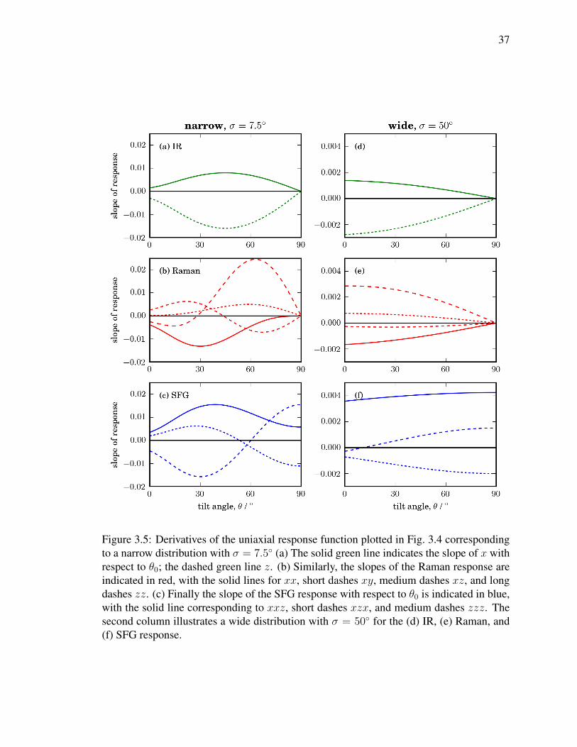
37

Figure 3.5: Derivatives of the uniaxial response function plotted in Fig. 3.4 correspondingto a narrow distribution with σ = 7.5 (a) The solid green line indicates the slope of x withrespect to θ0; the dashed green line z. (b) Similarly, the slopes of the Raman response areindicated in red, with the solid lines for xx, short dashes xy, medium dashes xz, and longdashes zz. (c) Finally the slope of the SFG response with respect to θ0 is indicated in blue,with the solid line corresponding to xxz, short dashes xzx, and medium dashes zzz. Thesecond column illustrates a wide distribution with σ = 50 for the (d) IR, (e) Raman, and(f) SFG response.

38

considering neighboring vibrational modes. Since the sign of the imaginary of χ(2) is

preserved, it provides orientation information that is not found in IR and Raman response.

For example, the fact that xxz < 0 and xzx > 0 tells the polarity of the orientation. To be

more precise, it allows us to determine if the molecules orient with 0 < θ0 < 90 or they

position upside down with 90 < θ0 < 180.

Spectra with multiple vibrational modes. So far I have only discussed spectrum with

single vibrational mode. Let’s consider a more complicated molecular response by taking

into account multiple vibrational modes. The theory behind the more complicated spectrum

is the same except that now polarizability derivative has 6 unique elements and dipole

moment derivative has 3 unique non-zero elements. Amino acid leucine is a good molecule

to study for comparison purpose since leucine’s vibrational response has been well studied,

including SFG [77, 78, 78, 79]. Leucine’s structure, along with its molecular frame is

illustrated in Fig. 3.3c. I used GAMESS package [71] with B3LYP/6-31G(d,p) to calculate

the dipole moment and polarizability derivatives. To approximate an aqueous solution

environment, a polarizable continuum is selected. Lorentzian line shapes were set to have

width of Γ = 10 cm−1, which is in agreement with experiment [78]. In light of the

experiment [77], Harmonic frequencies from a Hessian calculation were scaled by 0.945.

The results for methyl group orientation presented in the previous section compare

the three techniques with 8 different Gaussian distributions, four broad distribution (A-D)

and four narrow distributions (E-H), shown in the inset of Fig. 3.4. Similar approach is

applied to leucine molecule. I will start the discussion in broad distribution. The simulated

IR, Raman and SFG spectra of the broad distribution distributions (A–D) are shown in

Fig. 3.6 with aliphatic C-H stretching region 2800–3000 cm−1. A and B both have θ0 = 30

but different width. Similarly, C and D both have θ0 = 70 but different width. One

can immediately see that IR (top row) and Raman (middle row) both have spectra with

not much variation for the (A-D) distribution. Raman scattering arguably shows more

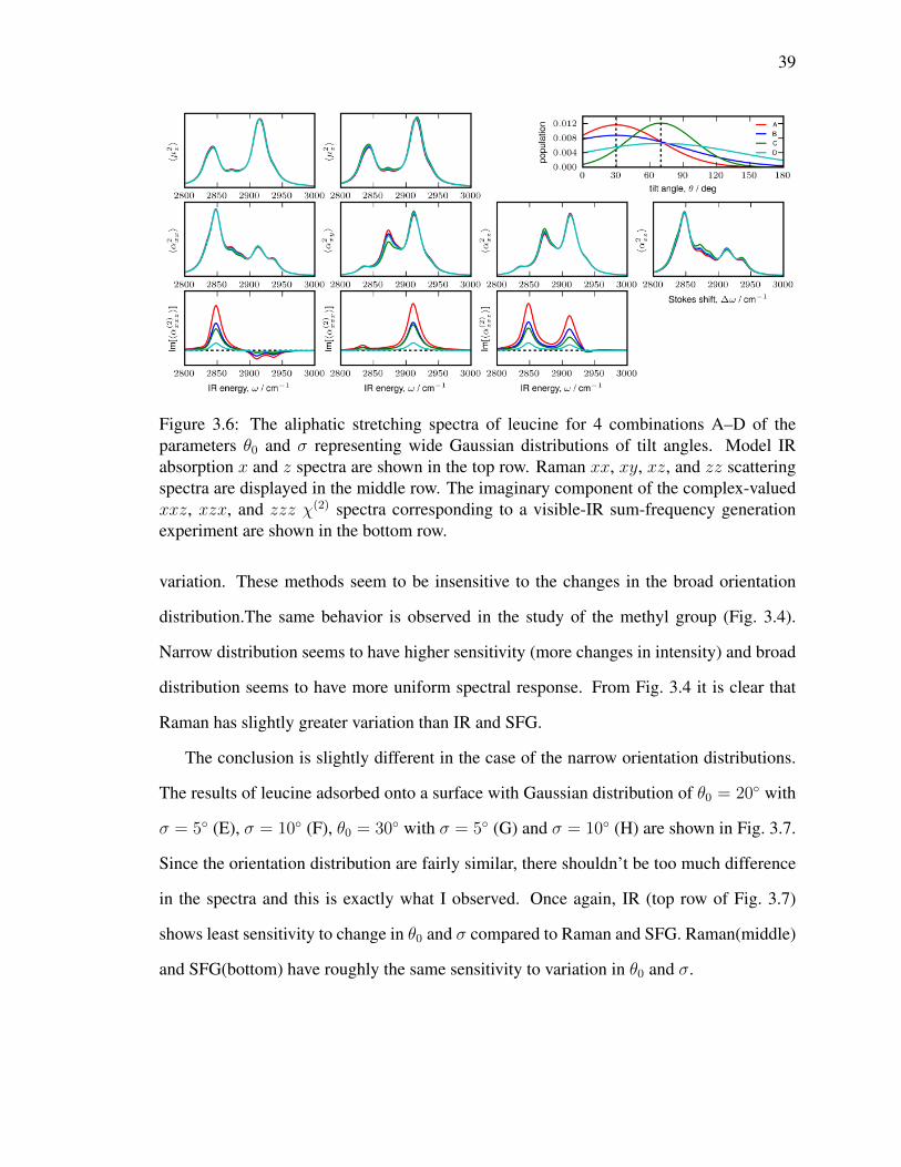
39

Figure 3.6: The aliphatic stretching spectra of leucine for 4 combinations A–D of theparameters θ0 and σ representing wide Gaussian distributions of tilt angles. Model IRabsorption x and z spectra are shown in the top row. Raman xx, xy, xz, and zz scatteringspectra are displayed in the middle row. The imaginary component of the complex-valuedxxz, xzx, and zzz χ(2) spectra corresponding to a visible-IR sum-frequency generationexperiment are shown in the bottom row.

variation. These methods seem to be insensitive to the changes in the broad orientation

distribution.The same behavior is observed in the study of the methyl group (Fig. 3.4).

Narrow distribution seems to have higher sensitivity (more changes in intensity) and broad

distribution seems to have more uniform spectral response. From Fig. 3.4 it is clear that

Raman has slightly greater variation than IR and SFG.

The conclusion is slightly different in the case of the narrow orientation distributions.

The results of leucine adsorbed onto a surface with Gaussian distribution of θ0 = 20 with

σ = 5 (E), σ = 10 (F), θ0 = 30 with σ = 5 (G) and σ = 10 (H) are shown in Fig. 3.7.

Since the orientation distribution are fairly similar, there shouldn’t be too much difference

in the spectra and this is exactly what I observed. Once again, IR (top row of Fig. 3.7)

shows least sensitivity to change in θ0 and σ compared to Raman and SFG. Raman(middle)

and SFG(bottom) have roughly the same sensitivity to variation in θ0 and σ.

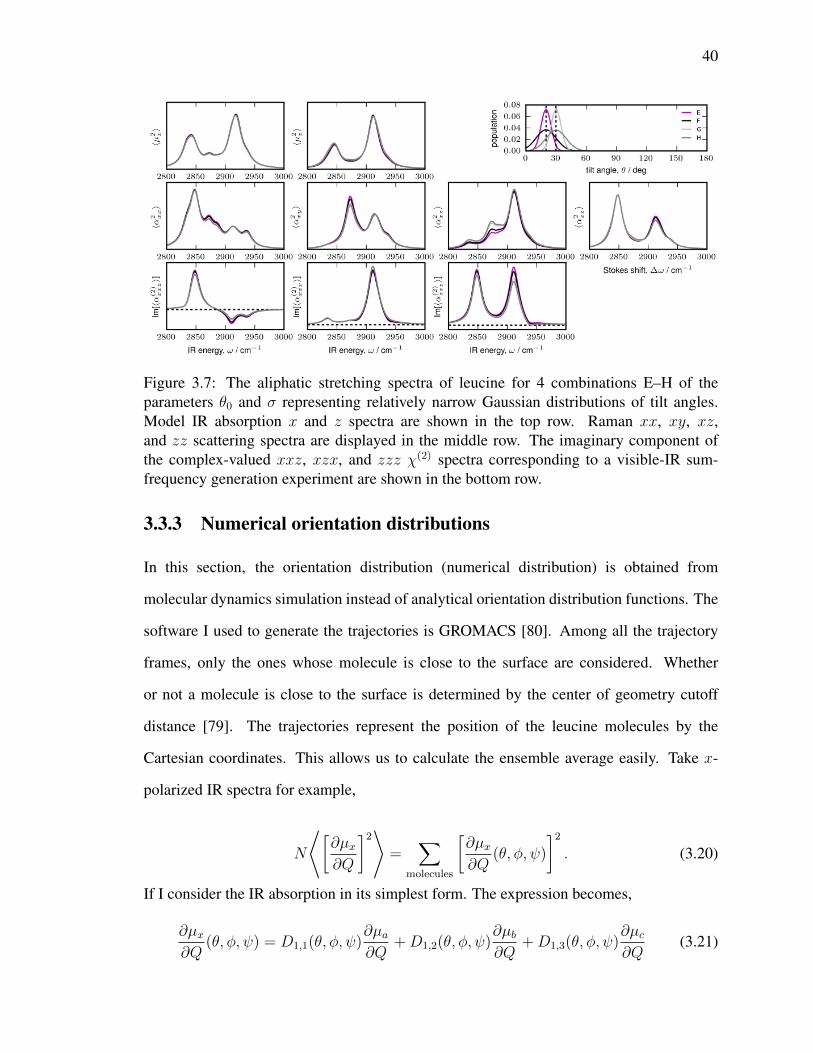
40

Figure 3.7: The aliphatic stretching spectra of leucine for 4 combinations E–H of theparameters θ0 and σ representing relatively narrow Gaussian distributions of tilt angles.Model IR absorption x and z spectra are shown in the top row. Raman xx, xy, xz,and zz scattering spectra are displayed in the middle row. The imaginary component ofthe complex-valued xxz, xzx, and zzz χ(2) spectra corresponding to a visible-IR sum-frequency generation experiment are shown in the bottom row.

3.3.3 Numerical orientation distributions

In this section, the orientation distribution (numerical distribution) is obtained from

molecular dynamics simulation instead of analytical orientation distribution functions. The

software I used to generate the trajectories is GROMACS [80]. Among all the trajectory

frames, only the ones whose molecule is close to the surface are considered. Whether

or not a molecule is close to the surface is determined by the center of geometry cutoff

distance [79]. The trajectories represent the position of the leucine molecules by the

Cartesian coordinates. This allows us to calculate the ensemble average easily. Take x-

polarized IR spectra for example,

N

⟨[∂µx∂Q

]2⟩

=∑

molecules

[∂µx∂Q

(θ, φ, ψ)

]2

. (3.20)

If I consider the IR absorption in its simplest form. The expression becomes,

∂µx∂Q

(θ, φ, ψ) = D1,1(θ, φ, ψ)∂µa∂Q

+D1,2(θ, φ, ψ)∂µb∂Q

+D1,3(θ, φ, ψ)∂µc∂Q

(3.21)

41

Figure 3.8: The aliphatic stretching spectra of leucine obtained from molecular dynamicssimulations of adsorption from solution onto two types of surfaces. Results for asuperhydrophobic surface (contact angle ≈ 150) are shown in blue; results for amoderately hydrophobic surface (contact angle ≈ 85) are shown in red. Model IRabsorption x and z spectra are shown in the top row. Raman xx, xy, xz, and zz scatteringspectra are displayed in the middle row. The imaginary component of the complex-valuedxxz, xzx, and zzz. χ(2) spectra corresponding to a visible-IR sum-frequency generationexperiment are shown in the bottom row.

where Dij are elements of the direction cosine matrix

D(θ, φ, ψ)

=

cosφ cos θ cosψ − sinφ sinψ − cosφ cos θ sinψ − sinφ cosψ sin θ cosφsinφ cos θ cosψ + cosφ sinψ − sinφ cos θ sinψ + cosφ cosψ sin θ sinφ

− cosψ sin θ sinψ sin θ cos θ

.(3.22)

I avoid calculating the Euler angles to express the lab-frame quantities by computing the

direction cosine matrix for each vibrational mode. Eq. 3.21 that the lab frame dipole

moment derivative is solely dependent on the elements of D, which is again dependent

on the Euler angle of the molecule. Note that dipole moment derivative is a constant in the

(a, b, c) molecular frame.

The blue spectroscopic response in Fig. 3.8 is a result of leucine adsorbed onto

superhydrophobic surface with its orientation distribution closely resembles Gaussian

42

distribution of tilt angles with θ0 ≈ 25 and σθ ≈ 20, twist angles with ψ0 ≈ 135

and σψ ≈ 80. The red spectroscopic response is the result of leucine adsorbed onto

moderately/minimally hydrophobic surface with complex orientation distribution in tilt (θ)

and twist (ψ). For the leucine molecules that are considered close to the surface, their

tilt (θ) and twist (ψ) angles are calculated. The aggregate results are shown in the inset of

Fig. 3.8. Fig. 3.8 shows that all three spectroscopic techniques are sensitive to the two (θ,ψ)

distribution that I picked. IR (top row) does show some variation in response intensity, but

the overall shape stays roughly the same. Raman (middle row) shows significant difference

expecially in in the xy- and zz-polarized components. SFG has the greatest sensitivity

among the three spectroscopic techniques as it shows appreciable differences in all three

elements of χ(2).

3.4 Conclusions

Nonlinear Spectroscopic techniques such as SFG has advantage over the linear spectro-

scopic techniques such as IR and Raman in that it is able to gather spectroscopic response

from the molecules that are ordered in a polar manner and ignore the spectroscopic response

from the molecules in the adjacent bulk phase. However, in the case where the molecules

being studied only present in the interfacial region and there is not need for adjacent

bulk discrimination IR and Raman are also viable alternatives that may even provide

richer structural information by probing the molecules with polarized light. Molecular

response tensor for each vibrational mode, the relative position of the chemical functional

groups within the molecule, the line shape and how the molecular properties (dipole

moment and polarizability) are projected into the lab frame all take part in determine the

sensitivity of the spectroscopic techniques to the orientational change. In this chapter,

I have discussed every one of the factors listed here by examining simple uniaxial

molecular response, symmetric stretch in methyl group with three-fold symmetry and C–H

stretching region of the leucine molecule. In these three scenarios, first they are examined

43

with analytical orientation distribution (Gaussian distribution) and then with numerical

orientation distribution which is gathered by sampling the molecular dynamics simulation

trajectory. Even though SFG is a the only surface specific spectroscopic technique that is

able to discriminate the adjacent bulk phase, in the scenario such as molecules adsorbed

on a surface where the bulk solution is absent, IR and Raman also provides molecular

orientation information. Lastly, all three techniques can be combined to reliably extract

molecular orientation distribution parameters and additional information.

44

Chapter 4

Linear Programming

4.1 Overview

Knowing which spectroscopy technique is sensitive to orientation change is important. It

enables us to generate a spectrum that is most rich in orientation distribution information.

However, it is a whole different story to extract orientation distribution information from

a vibrational spectrum. To extract the orientation distribution information, it involves

creating model spectrum with known orientation distribution. If the model spectrum

matches the experimental spectrum, they most likely carry the same orientation distribution

information. In Chapter 3, I illustrated how to make vibrational spectra and what they

look like. Now I am going to generate many spectra based on Gussian distribution with

different θ0 and θσ and call them candidates. Then I am going to combine them in a known

ratio to create model spectra and apply linear programming approach to see if the linear

programming approach can return the accurate ratio of the candidates.

4.2 Introduction

If I consider a spectrum as a polynomial function, it is really just a line constituted of an

infinite number of points with x and y values. If I denote the points in one spectrum as

(x1, y1) and the points in another spectrum as (x2, y2). The two spectra are identical if and

only if y1 = y2 when x1 = x2 or y1 − y2 = 0 when x1 − x2 = 0. That is, the points’ y

45

Figure 4.1: These are three figures to help explain the idea of sum of difference. A is thetarget. B and C are candidates. Three points selected in each figure to perform sum ofdifference.

value should the same if their x value is the same. It is easy to determine if two spectra

are identical because the criterion is straightforward. To determine the level of similarity

between spectra is another story. If I have spectra A, B and C, how do I determine between

B and C which one is more similar to A? A more advanced questions would be, what is

the best ratio of B and C that would produce a new spectrum closest to A. This is exactly

the question I want to answer here; how to find the best ratio of the candidates that best

fits the target spectrum. To say one ratio is better than the other, I must give each ratio

a score. I consider two approaches to obtain such a score; sum of differences and sum of

squared differences. Each method has its advantages and disadvantages along with different

statistical implication [81, 82].

The sum of differences approach sums up all the absolute differences in y value along

the x axis. Whichever candidate spectrum has the least sum of differences is the one most

similar to the target spectrum. The sum of differences between Fig. 4.1A and Fig. 4.1B is

|(2− 3)|+ |(3− 4)|+ |(3− 1)| = 4.

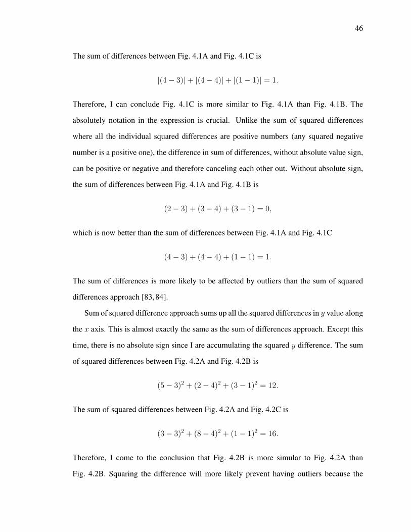
46

The sum of differences between Fig. 4.1A and Fig. 4.1C is

|(4− 3)|+ |(4− 4)|+ |(1− 1)| = 1.

Therefore, I can conclude Fig. 4.1C is more similar to Fig. 4.1A than Fig. 4.1B. The

absolutely notation in the expression is crucial. Unlike the sum of squared differences

where all the individual squared differences are positive numbers (any squared negative

number is a positive one), the difference in sum of differences, without absolute value sign,

can be positive or negative and therefore canceling each other out. Without absolute sign,

the sum of differences between Fig. 4.1A and Fig. 4.1B is

(2− 3) + (3− 4) + (3− 1) = 0,

which is now better than the sum of differences between Fig. 4.1A and Fig. 4.1C

(4− 3) + (4− 4) + (1− 1) = 1.

The sum of differences is more likely to be affected by outliers than the sum of squared

differences approach [83, 84].

Sum of squared difference approach sums up all the squared differences in y value along

the x axis. This is almost exactly the same as the sum of differences approach. Except this

time, there is no absolute sign since I are accumulating the squared y difference. The sum

of squared differences between Fig. 4.2A and Fig. 4.2B is

(5− 3)2 + (2− 4)2 + (3− 1)2 = 12.

The sum of squared differences between Fig. 4.2A and Fig. 4.2C is

(3− 3)2 + (8− 4)2 + (1− 1)2 = 16.

Therefore, I come to the conclusion that Fig. 4.2B is more simular to Fig. 4.2A than

Fig. 4.2B. Squaring the difference will more likely prevent having outliers because the

47

Figure 4.2: These are three figures to help explain the idea of sum of squared difference. Ais the target. B and C are candidate. Three points selected in each figure to perform sum ofsquared difference.

outliers are penalized heavily. In comparison, the sum of differences approach, the

difference between Fig. 4.2A and Fig. 4.2B is

|(5− 3)|+ |(2− 4)|+ |(3− 1)| = 6.

The differences between Fig. 4.2A and Fig. 4.2C is

|(3− 3)|+ |(8− 4)|+ |(1− 1)| = 4.

Fig. 4.2C now has better score than Fig. 4.2B. Although sum of squared difference is

favorable from the statistic point of view, the associated optimization technique, quadratic

programming, is far more computational intensive than linear programming and therefore

limiting the problem size [64].

If we search for the best ratio by calculating scores for all the possible ratios, it wouldn’t

scale well and examining more complex molecule/surface would be infeasible. Consider

the scenario where there are n candidates and the percentage is allocated to each candidate

48

in the granularity of 1%, the least percentage a candidate can have is 0% and the most

percentage a candidate can have is 100%. Finding out the total number of possible ratios

in this case is equivalent to finding all possible combination of 100 identical balls in n

non-identical bins. The answer to the question is

(100 + n− 1)!

100!(n− 1)!.

Therefore, even scoring takes constant time, the time complexity for the exhaustive

approach is still O(n!).

Since the exhaustive approach is not very appealing due to its complexity, I next turn to

mathematical programming. Mathematical programming is the selection of best element

among the alternatives. Since mathematical programming has been studied intensively,

a lot of efficient algorithms have been proposed and practiced. The hope is that, by

formulating the candidate ratio problem in a mathematical programming, I could take

advantage of the efficiency of the mathematical programming algorithm. Depending

on which scoring scheme is chosen, sum of difference or sum of squared difference,

the candidate ratio problem can be formulated as linear programming or quadratic

programming respectively. Because quadratic programming is far more computational

intensive than linear programming and therefore limiting the problem size, I choose linear

programming to solve candidate ratio problem.

Linear programming is an optimization technique to find optimum solutions for a

linear objective function under linear constraints. It is a special case of mathematical

programming whose constraint can be arbitrary degree of polynomial functions. Linear

constraints, whether it is linear equality or linear inequality constraints, collectively define

the region in n dimensional space in which all the possible solutions are defined. This

feasible region on a 2 dimensional space is often a polygon. The linear objective function’s

minimum or maximum happens at the vertices of the polygon. A linear programming

algorithm finds the vertex where the linear objective function has smallest or largest value

if it exists. The theory behind linear programming provides a way to drastically reduce the

49

Figure 4.3: All the possible solutions that satisfies the constraints are inside the gray area.The optimum solution happens at the vertices.

parameter space needs to be explored to determine the optimal solution. (See Fig. 4.3 for

example).

4.3 Linear Programming with inequality constraints

This section will show a simple linear programming example which involves inequality

constraints. The concepts and procedures shown here are directly applicable to formulating

candidate ratio problem as a linear program. Let us consider a simple example where the

to-be-minimized objective functions is

|x− 10|+ |y − 6|+ |z + 3|. (4.1)

This objective function, however, has a small problem. In the world of linear programming,

everything should be a linear function including objective function and constraints. Having

absolute signs in your function disqualifies it to be a linear function. Luckily, there is a

relatively simple way to take out the absolute signs from the objective function by adding

few more constrains. Two for each absolute value to be more precise.

If I want to minimize |x|, it is equivalent to minimize t with two constraints t ≥ x and

t ≥ −x. When x is a negative number, say -1, the constraints dictates that t ≥ −1 and

50

t ≥ −(−1) which causes t to be 1. This is correct because absolute value of -1 is indeed 1.

When x is a positive number, 1, the constraint dictates that t ≥ 1, t ≥ −1 which causes t

to be 1. This is also correct because absolute value of 1 is still 1. Therefore, no matter x is

greater or less than 0, I always have the desired value. Now that I establish the technique

to take out the absolute value sign from the linear function. Let us apply it to the objective

function 4.1.

For |x− 10|, let

X1 = |x− 10|

X1 ≥ x− 10 (4.2a)

X1 ≥ −x+ 10 (4.2b)

For |y − 6|, let

X2 = |y − 6|

X2 ≥ y − 6 (4.3a)

X2 ≥ −y + 6 (4.3b)

For |z + 3|, let

X3 = |z + 3|

X3 ≥ z + 3 (4.4a)

X3 ≥ −z − 3 (4.4b)

By letting t1, t2 and t3 represent each absolute value, the objective function to be minimized

now becomes

t1 + t2 + t3 (4.5)

with six constraints 4.2a - 4.4b.

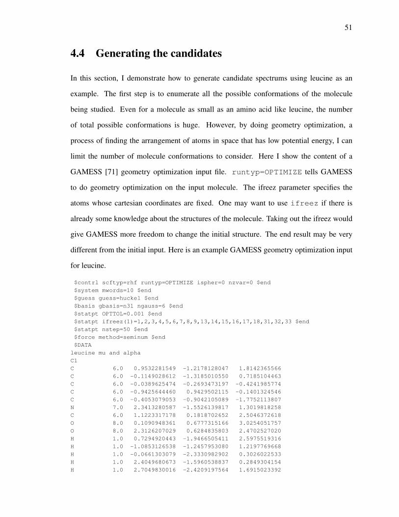
51

4.4 Generating the candidates

In this section, I demonstrate how to generate candidate spectrums using leucine as an

example. The first step is to enumerate all the possible conformations of the molecule

being studied. Even for a molecule as small as an amino acid like leucine, the number

of total possible conformations is huge. However, by doing geometry optimization, a

process of finding the arrangement of atoms in space that has low potential energy, I can

limit the number of molecule conformations to consider. Here I show the content of a

GAMESS [71] geometry optimization input file. runtyp=OPTIMIZE tells GAMESS

to do geometry optimization on the input molecule. The ifreez parameter specifies the

atoms whose cartesian coordinates are fixed. One may want to use ifreez if there is

already some knowledge about the structures of the molecule. Taking out the ifreez would

give GAMESS more freedom to change the initial structure. The end result may be very

different from the initial input. Here is an example GAMESS geometry optimization input

for leucine.

$contrl scftyp=rhf runtyp=OPTIMIZE ispher=0 nzvar=0 $end

$system mwords=10 $end

$guess guess=huckel $end

$basis gbasis=n31 ngauss=6 $end

$statpt OPTTOL=0.001 $end

$statpt ifreez(1)=1,2,3,4,5,6,7,8,9,13,14,15,16,17,18,31,32,33 $end

$statpt nstep=50 $end

$force method=seminum $end

$DATA

leucine mu and alpha

C1

C 6.0 0.9532281549 -1.2178128047 1.8142365566

C 6.0 -0.1149028612 -1.3185010550 0.7185104463

C 6.0 -0.0389625474 -0.2693473197 -0.4241985774

C 6.0 -0.9425644460 0.9429502115 -0.1401324546

C 6.0 -0.4053079053 -0.9042105089 -1.7752113807

N 7.0 2.3413280587 -1.5526139817 1.3019818258

C 6.0 1.1223317178 0.1818702652 2.5046372618

O 8.0 0.1090948361 0.6777315166 3.0254051757

O 8.0 2.3126207029 0.6284835803 2.4702527020

H 1.0 0.7294920443 -1.9466505411 2.5975519316

H 1.0 -1.0853126538 -1.2457953080 1.2197769668

H 1.0 -0.0661303079 -2.3330982902 0.3026022533

H 1.0 2.4049680673 -1.5960538837 0.2849304154

H 1.0 2.7049830016 -2.4209197564 1.6915023392

52

H 1.0 2.8624743345 -0.6924557806 1.6767353227

H 1.0 0.9961898439 0.0983591282 -0.5006749995

H 1.0 -0.8161334887 1.7137851886 -0.9082518288

H 1.0 -0.7317827535 1.3805339291 0.8384528790

H 1.0 -1.9958591030 0.6340267584 -0.1471630607

H 1.0 -0.3736111792 -0.1606071906 -2.5788293493

H 1.0 0.2782305563 -1.7177411715 -2.0422388509

H 1.0 -1.4199240724 -1.3196029859 -1.7451355742

$END

After the geometry optimization, the next step is to do Hessian calculation. The Hessian

calculation tells us the number vibrational modes and associated displacement from the

equilibrium state. Again, the program I choose to do the calculation is GAMESS. The

header for the GAMESS electronic structure calculation is very similar to that of geometry

optimization file. The major difference is that RUNTYP is now HESSIAN instead of

OPTIMIZE. Here is an example GAMESS Hessian calculation input for leucine.

$contrl scftyp=rhf runtyp=Hessian nosym=1 ispher=0 $end

$system mwords=10 $end

$DFT dfttyp=b3lyp $end

$guess guess=huckel $end

$basis gbasis=n31 ngauss=6 npfunc=1 ndfunc=1 $end

$PCM solvnt=water $end

$force method=seminum $end

$DATA

leucine mu and alpha

C1

C 6.0 0.9532281549 -1.2178128047 1.8142365566

C 6.0 -0.1149028612 -1.3185010550 0.7185104463

C 6.0 -0.0389625474 -0.2693473197 -0.4241985774

C 6.0 -0.9425644460 0.9429502115 -0.1401324546

C 6.0 -0.4053079053 -0.9042105089 -1.7752113807

N 7.0 2.3413280587 -1.5526139817 1.3019818258

C 6.0 1.1223317178 0.1818702652 2.5046372618

O 8.0 0.1090948361 0.6777315166 3.0254051757

O 8.0 2.3126207029 0.6284835803 2.4702527020

H 1.0 0.7294920443 -1.9466505411 2.5975519316

H 1.0 -1.0853126538 -1.2457953080 1.2197769668

H 1.0 -0.0661303079 -2.3330982902 0.3026022533

H 1.0 2.4049680673 -1.5960538837 0.2849304154

H 1.0 2.7049830016 -2.4209197564 1.6915023392

H 1.0 2.8624743345 -0.6924557806 1.6767353227

H 1.0 0.9961898439 0.0983591282 -0.5006749995

H 1.0 -0.8161334887 1.7137851886 -0.9082518288

H 1.0 -0.7317827535 1.3805339291 0.8384528790

H 1.0 -1.9958591030 0.6340267584 -0.1471630607

H 1.0 -0.3736111792 -0.1606071906 -2.5788293493

53

H 1.0 0.2782305563 -1.7177411715 -2.0422388509

H 1.0 -1.4199240724 -1.3196029859 -1.7451355742

$END

The Hessian calculation result is in pure text format. For the resutls to be usable for

the programs, I need to parse the output. The python script parse.py is created for this

purpose. The results will be parsed into Python pickle file. In Python, pickling is a standard

way to serialize data. Run the following command to parse the output file

python parse.py <Gamess output file name>

<pickle file name>.pkl

To access the frequency for each mode: Frequency[mode]

Frequency[0] returns the frequency of model

Frequency[40] returns the frequency of mode41

To access the equilibrium coordinates: Coordinates[xyz][atom]

Coordinates[0][0] access the x coordinate of atom1

Coordinates[1][2] access the y coordinate of atom3

Coordinates[2][35] access the z coordinate of atom36

To access the displacement of an atom in x, y, z direction in each vibration mode:

Displacement [mode][xyz][atom]

Displacement[0][0][0] access the displacement of mode1

in x coordinate of atom1

The rest of the information stored in the pickle file are AtomType, ReducedMass and

AtomCharge. The way to access them is similar to that of frequency. The information

are stored into a pickle file in the order of frequency, coordinates, displacement, atomtype,

reducedmass and atomCharge. When the pickle file is unloaded, the information is

unloaded the same order.

54

A specific vibrational mode indicates the molecule vibrates in a certain way, described

by the x, y, z displacement from the equilibrium state of each atom. Dipole moment

and polarizability both change as the shape of the molecule changes. Calculate the dipole

moment and polarizability at different moment of the vibration, interpolate the value,

calculate the rate of changing at equilibrium state and I now have the dipole moment

derivative and polarizability derivative.

In practice, each vibrational mode has 7 snapshots, which represent each differ-

ent state the molecule can assume during the mode vibration. The python script

create input files.py is created to do the job. This script will create multiple

GAMESS input files (7 in this case) based on the information in pickle file from the Hessian

calculation. The run type for each GAMESS job is runtyp=ffield. This run type

does the electronic calculation and return dipole moment and polarizability. The following

shows how to run the script. The first argument is the pickle file; second argument is

starting mode number; third number is ending mode number; fourth argument is part of the

name of the input file.

python create_input_files.py

<Hessian calculation result pickle>.pkl

<start mode number> <end node number>

<file header>

After the last step, I obtained 7 dipole moments and polarizabilities for each mode. I

interpolate those values with second degree polynomial plot and calculate the rate of change

at equilibrium point to get the derivative of dipole moment and polarizability for each mode.

read output files.py takes care of all that. The first argument is the output pickle

file name. Second argument is the name header of GAMESS output file from last step.

For example, if the output file names are of the form glu mode X point X.out then put

glu. Third argument is the dipole moment derivative pickle file name you want. The fourth

argument and fifth argument specifies the starting mode and ending mode number inclusive.

55

python read_output_files.py

<Hessian calculation result pickle>.pkl <file header>

<dipole moment/polarizability derivatives output file>.pkl

<start mode number> <end node number>

Now that all the necessary pieces (dipole moment derivative and polarizability derivative)

are gathered, I can finally create the candidate spectrum. Instead of doing MD simulation

and project derivatives from molecular frame to lab frame. I leverage orientation distribu-

tion function (Normal/Gaussian distribution). Use spectrum orientation distr

ibution analyticalMeshgrid.py to generate analytical spectrum. Here is the

usage to this script:

python

spectrum_orientation_distribution_analyticalMeshgrid.py

<dipole moment/polarizability derivatives output file>.pkl

<output file name>.pkl

<theta0=x> <thetasigma=y> <psi0=x> <psisigma=y>

<thetaonly=true/false>

This script assumes uniformly distributed φ and/or ψ. theta0 defines the average in the θ

normal distribution. thetasigma defines θσ in the θ normal distribution. psi0 defines the

average in the ψ normal distribution. psisigma defines ψσ in the ψ normal distribution.

If thetaonly is set to true, this means I assume an uniform distribution in both φ and ψ.

The candidate spectrum is stored in a pickle file. Fig. 4.4 shows an example of alanine

candidates.

4.5 Combining the candidates

As demostrated I can compare candidates with the target spectrum by applying sum of

differences technique to find which single candidate is most similar to the target spectrum.

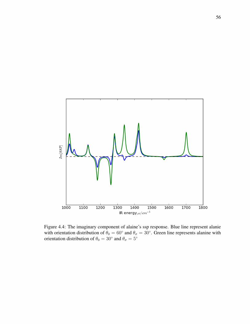
56

Figure 4.4: The imaginary component of alaine’s ssp response. Blue line represent alaniewith orientation distribution of θ0 = 60 and θσ = 30. Green line represents alanine withorientation distribution of θ0 = 30 and θσ = 5

57

It is a problem that requires little computational power. The running time is O(n).

However, it is not quite what I want. In real life, molecules don’t orient on a surface

in a single way. They orient in different ways with different population. Therefore,

the candidates should not be considered individually. I should instead consider different

combinations of the candidates spectra to find the best match to the target spectrum.

Let us consider m sample points in n candidates spectra whose population is denoted

as X1, X2, X3 ... Xn and the functions to represent each candidate spectrum as

f1(x), f2(x), f3(x)...fn(x), the function to represent target spectrum is f0(x). Because

the final population is always 100%, the population for each candidate spectrum will add

up to one, X1 + X2 + X3 + ...Xn = 1. When m = 1, meaning only one sample point

is picked, the expression for calculating sum of differences for each candidate population

combination is |f0(x1)− (X1 · f1(x1) +X2 · f2(x1) +X3 · f3(x1) + ...Xn · fn(x1))|. In a

more general form where there are m sample points, I have

|f0(x1)− (X1 · f1(x1) +X2 · f2(x1) +X3 · f3(x1) + ...Xn · fn(x1))|+



|f0(x2)− (X1 · f1(x3) +X2 · f2(x3) +X3 · f3(x3) + ...Xn · fn(x3))|+...

|f0(xm)− (X1 · f1(xm) +X2 · f2(xm) +X3 · f3(xm) + ...Xn · fn(xm))|

(4.6)

The compact form ispoints∑p=1

∣∣∣∣∣Im[χ(2)]p −candidates∑

c=1

fc · Im[χ(2)]c,p

∣∣∣∣∣ (4.7)

I can take out the absolute sign as demostrated in section 4.3. Let t1, t2, t3, ..., tm represent

each of the absolute value and the objective function becomes

t1 + t2 + t3 + ...+ tm (4.8)

. This is the constraint due to the fact that the ratio adds up to 1 (or 100%)

X1 +X2 +X3 + ...+Xn = 1 (4.9)

58

These constraints are the byproduct of getting rid of the absolute sign.

t1 −X1 · f1(x1)−X2 · f2(x1)−X3 · f3(x1)− ...Xn · fn(x1) ≥ −f0(x1)

t1 +X1 · f1(x1) +X2 · f2(x1) +X3 · f3(x1) + ...Xn · fn(x1) ≥ f0(x1)

...

tn −X1 · f1(xn)−X2 · f2(xn)−X3 · f3(xn)− ...Xn · fn(xn) ≥ −f0(xn)

tn +X1 · f1(xn) +X2 · f2(xn) +X3 · f3(xn) + ...Xn · fn(xn) ≥ f0(xn)

(4.10)

In the end, we have a linear program with one objective function and 2m+ 1 constraints.

If I do this exhaustively, i.e. calculating the sum of differences for all possible

combinations of the candidates, the problem space will be too big to compute. Assuming

the population percentage is allocated wholly, the total possible number of combination

among n candidates will be(100 + n− 1)!

100!(n− 1)!.

This leads the running time of solving the problem toO(n!), which is infeasible to compute

even for moderate size n . The number of sample points picked to calculate sum of

differences also impacts the performance. Picking too many sample points requires too

much computational power. However, If the number of sample points are too few, then the

final answer may not be very accurate. How many points in a figure should I consider for

calculating sum of differences? There is no single answer that fits all scenarios. Please

consult NyquistShannon sampling theorem for sampling guidance [85].

I now have established the goal is to model the (target) experimental spectra based of

the linear combinations of the candidates. Each candidate is a spectrum whose orientation

distribution and electronic structure properties are known. For example, I could have a

spectrum candidate in which the species is leucine with Gaussian distribution of θ0 = 30

and θσ = 5. Choosing candidates is important. If I consider too many variables, the

number of candidate could grow exponentially. For instance, consider one conformer of

leucine with delta distribution on tilt and twist angle in 1 step. I will easily have 180x360

= 64800 candidates. No matter how many candidates are there, the final population is

59

always 100 %. For example, I have three candidates a, b, c with population A, B, C, then

A+B + C = 1. One possible answer is A = 0.6, B = 0.3 and C = 0.1. This means 60%

of a, 30% of b and 10% of c. It is absolutely possible for a candidate to have population

zero in the final answer. As a matter of fact, since the number of candidates is generally

big, most of the candidate’s population will be zero or nearly zero.

4.6 Differential weighting of candidate sampling points

For the mathematical expression shown in Fig. 4.6, it is assumed that the difference at all

the data points are weighed equally. However, in some scenarios, some data points should

be weighed more heavily than the other ones. For example, if there are features (peaks and

valley) in a spectrum which one deems important, I can put more weight on the data points

reside in those regions by introducing a1, a2....am in front of each elements in function 4.6.

The expression now becomes Fig. 4.11. For example, if a1 is 10 and a2 is 1, this means

data point a1 is weighed 10 times more than a2. When the weight factor a1, a2...am is 1 for

all the data points, all the data points are weighed equally.

a1 · |f0(x1)− (X1 · f1(x1) +X2 · f2(x1) +X3 · f3(x1) + ...Xn · fn(x1))|+

a2 · |f0(x2)− (X1 · f1(x2) +X2 · f2(x2) +X3 · f3(x2) + ...Xn · fn(x2))|+

a3 · |f0(x2)− (X1 · f1(x3) +X2 · f2(x3) +X3 · f3(x3) + ...Xn · fn(x3))|+...

am · |f0(xm)− (X1 · f1(xm) +X2 · f2(xm) +X3 · f3(xm) + ...Xn · fn(xm))|

(4.11)

In this thesis, I treated all the points in the spectra to be equal. However, this is a

important technique to be noted. In the later of this chapter I will show that some of the

spectra region is more sensitive to the orientational changes. Therefore, if we put more

weights on the points reside in that region, more accurate results could be achieved.

60

4.7 GNU linear programming tool kit

The tool I choose to carry out Linear programming is called “GNU linear programming

tool kit” (GLPK). It is written in ACNSI C and is intended for solving large scale linear

programming. The format in which I represent our linear program is CPLEX format.

Another possible format is MPS. GLPSOL, the GLPK command-line solver is capable

of consuming this type of input format and carrying out linear programming optimization.

For example, the linear programming problem in Func 4.1 can be represented as follows

Minimize

objective: T1 + T2 + T3

Subject To

constraint0: T1 - x >= -10

constraint1: T1 + x >= +10

constraint2: T2 - y >= -6

constraint3: T2 + y >= +6

constraint4: T3 - z >= +3

constraint5: T3 + z >= -3

Bounds

- infinity <= x <= + infinity

- infinity <= y <= + infinity

- infinity <= z <= + infinity

End

Bounds

- infinity <= x <= + infinity

- infinity <= y <= + infinity

- infinity <= z <= + infinity

61

End

If the input is saved as test.lp, run the following command. The output is saved as

test.out.

glpsol -o test.out --lp test.lp

It is necessary to specify the bounds of x, y, z to be between positive and negative infinity.The default lower bound is zero and the default upper bound is positive infinity. The defaultwill remain in effect until the bound is explicitly changed. Here is the output:

Output:

Problem:

Rows: 6

Columns: 6

Non-zeros: 12

Status: OPTIMAL

Objective: objective = 0 (MINimum)

No. Row name St Activity Lower bound Upper bound Marginal

------ ------------ -- ------------- ------------- ------------- -------------

1 constraint0 NL -10 -10 0.5

2 constraint1 NL 10 10 0.5





No. Column name St Activity Lower bound Upper bound Marginal

------ ------------ -- ------------- ------------- ------------- -------------

1 T1 B 0 0

2 T2 B 0 0

3 T3 B 0 0

4 x B 10

5 y B 6

6 z B -3

Karush-Kuhn-Tucker optimality conditions:

KKT.PE: max.abs.err = 0.00e+00 on row 0

max.rel.err = 0.00e+00 on row 0

High quality

KKT.PB: max.abs.err = 0.00e+00 on row 0


High quality

KKT.DE: max.abs.err = 0.00e+00 on column 0

max.rel.err = 0.00e+00 on column 0

High quality

KKT.DB: max.abs.err = 0.00e+00 on row 0

62


High quality

End of output

The optimal solution to the linear programming is listed above. As one can see, T1, T2,

and T3 are zeros. This is as a result of x = 10, y = 6 and z = −3. The last section is called

Karush-Kuhn-Tucker optimality conditions [86, 87]. They are necessary and sufficient for

the given solution to be a global optimum.

4.8 Methods and Implementation

4.8.1 Making SFG pickle files for linear programming

A SFG pickle file contains necessary information to create a SFG spectrum. spectrum

orientation distribution analyticalMeshgrid.py will generate such

pickle file given necessary parameter from command line such as θ angle, ψ angle and the

dipole property pickle file of the molecule being studied. Because the number of candidates

is big and I am creating a SFG pickle file for each candidate, it is inefficient to create

them one by one on a terminal. I use make theta psi analytical pickles.sh to

generate those SFG pickle files. make theta psi analytical pickles.shwill in

turn calls spectrum orientation distribution analyticalMeshgrid.py

with different θ and ψ value. Make sure spectrum orientation distribution

analyticalMeshgrid.py is up-to date.

make theta psi analytical pickles.sh can create mulitple pickles with

different θ0 and ψ0 all with delta distribution. However, the script can be changed to create

pickle file with gaussian distribution as well. There is another scrip make theta analyt

ical pickles.sh that does the same thing except for it’s θ only. Details for how to

generate dipoleproperty pickle file, please refer to the previous document.

63

4.8.2 The experimental data file

All of the pickle files generated from the last step are the candidates. I want to know

what combinations/percentage of each candidates will reproduce the experimental SFG

spectrum.The experimental data file consists of four columns. The columns, from left to

right, represents wavelength, ssp, sps and ppp. Use getData.py to print the data points

to standard output (POINTS PICKED is defined in fresnelsMicro.py) This script

will print to stdout the y values of the experimental spectrum at POINTS PICKED and is

an auxiliary script used by makeLP.py. You most likely won’t use this script directly.

python getData.py <dataFileName> <sps/ssp/ppp/all>

With all option, the script will print out all three polarization in the order of ssp, sps and

ppp. so the number of values being printed out is POINTS PICKED*3

4.8.3 Linear Programming Text Input

This is the final step before creating CPLEX LP input for GLPSOL. The linear pro-

gramming text input contains the number of the candidates, the number of the sample

points, the location of the candidate files, the y values of the data points in target and

in each candidates.The first line of the linear programming text input are two numbers.

The first number is the number of candidates. The second number is the number of data

points being sampled and it should be the same as POINTS PICKED which is defined in

fresnelsMicro.py. The second line are the y values of the experimental spectrum at

POINTS PICKED. The first two lines are taken care of by the makeLP.py.

python makeLP.py <dataFileName> <number cadidates>

<number points picked> <ssp/sps/ppp/all>

The rest of the lines starts with the location of the pickle file of each candidate followed

by the y values of the experimental spectrum at POINTS PICKED. The rest of the lines

64

are filled by completeLP.sh which in turn calls makeLPinputFromPickel.py. Here

is the example of calling completeLP.sh.

completeLP.sh lp.txt ssp

Note that the location of the pickle files and the pattern of the name of the pickle files are

still hard-coded. Here is the example of the linear programming text input. There are 2

candidates in total and the number of sample points is 3.

2 3

1 2 3

candidates/candidate1.pkl 1 1 1

candidates/candidate2.pkl 3 2 1

4.8.4 Linear Programming Input and Output

realProblemSolver.pywill parse the linear programming text input into CPLEX LP

format.

realProblemSolver.py <linrear programming input> <outputfile>

Linear Programming Calculation with GLPSOL

glpsol -o <output file> --lp <CPLEX LP input file>

In the output file, there lies the answer.

4.8.5 Plotting Result

As a result of the previous step, I now know what is the best, or at least optimal combina-

tion/percentage of the candidates to reconstruct the target spectrum. plotResultByPo

pulation.sh draws the spectrum based on the answer given the linear programming

output file. It does this by parsing the linear programming output file and pass the

information to plotResultByPopulation.py.

65

4.9 Results and Discussion

I have established the theory and implementation details in the previous chapters. The next

step is to see if the linear programming approach indeed returns the optimal solution or

a near optimal solution. It is not practical to use experimental spectra as target spectra

because the orientation distribution is usually unknown. Instead, the target spectra is made

up with known candidates and known orientation distribution. This allows us to evaluate

the accuracy of the answer that linear programming returns.

4.9.1 Delta distributions

All of the candidates created in this section assume delta distribution. Delta distribution, in

this context, means all of the population has the same orientation and has no deviation at all.

Different amino acids, θ0 only. The target spectrum presented here is θ only with delta

distribution. It consists of 34% alanine with θ0 = 20, 12% isoleucine with θ0 = 30 and

54% methionine with θ0 = 40. 2001 data points are picked evenly between 1000 cm−1

and 3000 cm−1, ssp only. With this setting, the linear programming solver is able to find

right combination of among candidates to match the target spectrum. The candidates are

alanine, isoleucine, methionine, lysine, valine and threonine with θ0 from 10 to 180 in

10 step. Linear programming returns the right answer. The result is represented visually

in Fig. 4.5. As one can see, the bottom panel is zero across all data point. This means that

linear programming returns the perfect answer.

Different amino acids, θ0 and ψ0. The target spectrum presented here is both θ and ψ

with delta distribution. It is consisted of 34% alanine with θ0 = 30 and ψ0 = 10,

12% isoleucine with θ0 = 50 and ψ0 = 250, 54% methionine with θ0 = 110 and

ψ0 = 150. 2001 data points are picked evenly between 1000−1 and 3000 cm−1, ssp

only. With this setting, the linear programming solver is able to find right combination

66

Figure 4.5: The top panel show the spectrum that linear programming returns. The bottompanel show the difference between the result that linear programming returns and the actualspectrum.

67


among 972 candidates to match the target spectrum. The candidates are alanine, isoleucine,

methionine, lysine, valine and threonine with θ0 from10 to 170 in 20 step and ψ0 from

10 to 350 in 20 step. Again, linear programming returns the correct answer. The result

is represented visually in Fig. 4.6.

Same amino acids, different degree in θ0. The target spectrum presented here is θ only

with delta distribution. It is consisted of 34 % alanine with θ0 = 20, 12% alanine with

θ0 = 30 and 54% alanine with θ0 = 40. The 2001 data points are picked evenly between

1000 cm−1 and 3000 cm−1, ssp only.

With this setting, the linear programming solver is not able to find right combination of

68


108 candidates to match the target spectrum. The candidates are 18 of alanine, isoleucine,

methionine, lysine, valine and threonine each at various degree in θ. The returned answer

from linear programming solver is 3.0% alanine with θ0 = 10, 82.3% alanine with θ0 =

30 and 14.6% alanine with θ0 = 50. Although the answer is incorrect, it is worth noting

that the species is correct. They are all alanine. The result is represented visually in Fig. 4.7.

4.9.2 Gaussian distribution, theta only

Different amino acids, different degree in θ0. The target spectrum presented here is theta

only with delta distribution. It is consisted of 34% alanine with θ0 = 40 and θσ = 5, 12%

isoleucine with θ0 = 130 and θσ = 30 and 54% methionine with θ = 170 and θσ = 5.

2001 data points are picked evenly between frequency 1000 and 3000 cm−1, ssp only.

69

Figure 4.8: Linear programming solver does not return the optimal solution. The bottompanel show the difference at each data point. As one can see, there are some difference atsome data points. This indicates the returned answer is not perfect.

With this setting, the linear programming solver is not able to find right combination of

180 candidates to match the target spectrum. The candidates are 30 of alanine, isoleucine,

methionine, lysine, valine and threonine each at various degree in θ and various degree in

θσ. The returned answer from linear programming solver is 10.2 % alanine with θ0 = 20

and θσ = 5 , 25.5% alanine with θ0 = 50 and θσ = 5 , 7.0% isoleucine with θ0 = 130

and θσ = 5 , 0.8% isoleucine with θ0 = 170 and θσ = 5 , 1.4% methionine with θ = 60

and θσ = 5, 33.5% methionine with θ0 = 180 and θσ = 5 and 21.6% methionine with

θ0 = 160 and θσ = 5 . By grouping the percentages by species, I have alanine 35.8%,

isoleucine 7.764% and methionine 56.4%. The population for each species is roughly

correct. The result is represent visually in Fig. 4.8

70

4.9.3 Discussion

In the case of delta distribution, whether it’s theta only or both theta and psi, the linear

programming solver is always able to get the correct solution when the target spectrum

consisted of different molecules (i.e. no same molecules with different orientation). See

Fig. 4.5 and Fig. 4.6. I then turned to see if the linear programming solver is able to

return the optimal solution when the target spectrum consisted of candidates which are the

same molecule but has different orientation. This is supposedly a harder problem because

candidates that are the same molecule with different orientation are much more similar to

each other than they are when the candidates are different molecules. Unfortunately, the

linear programming solver did not return the optimal solution in the case of Fig. 4.7.

It is a success when the target spectrum consisted of different molecules (i.e. no

same molecules with different orientation) in the case of delta distribution. The linear

programming solver is able to find the optimal solution. Same condition for the target

spectrum (i.e. no same molecules with different orientation) in the case of Gaussian

distribution. This time the linear programming solver failed to return the optimal solution.

However, the linear programming solver did return roughly the correct population by

molecule.

Scaling the intensity. One of the theory behind the linear programming solver unable to

find the optimal solution in some scenarios (e.g. Same amino acids, different degree in

theta) is because each candidate’s intensity is too small. If I examine Fig. 4.5, Fig. 4.6,

Fig. 4.7 and Fig. 4.8 carefully, it is not hard to see the intensities are in the neighborhood

of 10−3 and 10−4. The difference at each data point is even smaller, between 10−10 and

10−9. Perhaps the diminutiveness of the spectrum for each candidate hinders the linear

programming solver’s ability to give right answers. I attempted to prove this theory by

increasing intensity of the target spectrums and candidates by various magnitude.

Looking at the results presented in Fig. 4.1, it is difficult to say that the accuracy

71

AA true scale 1 scale 10 scale 100 scale 1K scale 10KAla 0.150 0.151 0.151 0.151 0.155 0.150Ile 0.100 0.114 0.114 0.114 0.109 0.091Thr 0.150 0.150 0.150 0.150 0.150 0.184Met 0.330 0.273 0.273 0.273 0.274 0.305Val 0.270 0.312 0.312 0.312 0.312 0.270total 1.000 1.000 1.000 1.000 1.000 1.000

Table 4.1: This shows whether or not the linear programming solver returns more accurateresults as the intensity magnitude increases. The true column shows what the correctanswer should be. The other columns show the answer that linear programming solverreturns at different intensity scaling.

increases as the intensity magnitude increases. However, it is clearly that the linear

programming solver returns different answers as the magnitude changes. Investigating

further into the relation between intensity magnitude and linear programming would shed

more lights on how to make linear programming solver return more accurate answers.

Narrow/Wide distributions. Linear programming works the best when the candidates

are drastically different from one another. The results presented in section 4.9.2 suggests

that linear programming could not differentiate candidates if they only differ in θσ. This

could also mean that at some scenarios, candidates which differ only in θσ may look very

similar. Here I investigate the difference between narrow(θσ = 5) and wide (θσ = 30)

distribution for the amino acids I study. The first amino acid I look at is the alanine. From

Fig. 4.9, I can clearly see that the difference is nearly 0 for wave number 1000 cm−1 to

1200 cm−1and 1400 cm−1 to 1800 cm−1 for ppp, sps and ssp and all three polarizations.

sps shows most difference between wave number 1200 cm−1 to 1400 cm−1 and θ0 = 60 to

θ0 = 90. ppp and ssp shows most difference in the same wave number region, 1200 cm−1

to 1400 cm−1 but with θ0 = 0 to θ0 = 30. If I consider ppp, ssp and sps together (Fig. 4.9

bottom panel), the most difference region is still between wave number, 1200 cm−1 to

1400 cm−1 and θ0 = 0 to θ0 = 30. This is not surprising considering two of three

polarization’s most difference region is there. Coming up is isoleucine. ssp, sps and ppp all

72

show noticeable difference at wavenumbers 1060 cm−1, 1210 cm−1, 1340 cm−1 between

θ0 = 60 to θ0 = 90 and θ0 = 0 to θ0 = 40. Besides those wavenumbers, ssp also

has two more bands at wave number 1280 cm−1 and 1460 cm−1. The last amino acid

to examine is methionine. sps and ppp have very similar bad patterns. They all show

significant differences at wave number 1080 cm−1 and 1450 cm−1 between θ0 = 0 to

θ0 = 35 and θ0 = 60 to θ0 = 90. ssp shows great difference at the same wave numbers,

but only between θ0 = 0 to θ0 = 35. The ssp spectrum also shows a band that is not seen

in sps and ppp at wave number 1550 cm−1 between θ0 = 60 to θ0 = 90. Having know the

region where most difference happens helps us to decide which points to put more weights

on. This could theoretically increases the accuracy of the result linear programming returns.

4.10 Conclusions

Doing an exhaustive search among the candidates to find the right combination that best

matches the experimental spectrum is intuitive and accurate. However, the running time

for the exhaustive approach is O(n!), which is even worse than the exponential growth

rate. Therefore, it doesn’t scale and prevents us from examining the spectrum for large

size molecules. By formulating the problem as linear programming, the running time is

now drastically reduced to pseudo O(n) and I can therefore consider more parameters and

examine spectrum of bigger molecules. To evaluate the accuracy of the linear programming

approach, mock spectra for IR, Raman and SFG are made with known ration of the

candidates and apply linear programming to see if the results is the same as the known

ratio. In the case where the candidates are delta distribution, linear programming is able to

return the right ratio when the mock spectra is constituted of different species even when

considering both θ and ψ Euler angles. However, when the mock spectra is made out of

candidates of same species, linear programming returns the right specie but with wrong

orientation distribution. In the case of broad distribution, linear programming does not

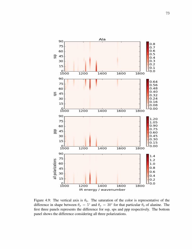
73

Figure 4.9: The vertical axis is θ0. The saturation of the color is representative of thedifference in shape between θσ = 5 and θσ = 30 for that particular θ0 of alanine. Thefirst three panels represents the difference for ssp, sps and ppp respectively. The bottompanel shows the difference considering all three polarizations.

74

Figure 4.10: The vertical axis is θ0. The saturation of the color is representative of thedifference in shape between θσ = 5 and θσ = 30 for that particular θ0 of Isoleucine. Thefirst three panels represents the difference for ssp, sps and ppp respectively. The bottompanel shows the difference considering all three polarizations.

75

Figure 4.11: The vertical axis is θ0. The saturation of the color is representative of thedifference in shape between θσ = 5 and θσ = 30 for that particular θ0 of methionine. Thefirst three panels represents the difference for ssp, sps and ppp respectively. The bottompanel shows the difference considering all three polarizations.

76

return the perfect answer like it did in the case of delta distribution. Nonetheless, it is still

worth noting that the linear programming solver does return roughly the right ratio in terms

of species.

77

Chapter 5

Summary and future work

5.1 Summary

Extracting quantitative orientation information from the spectra often involves creating

a model spectra from the candidates that closely resemble, if not identical, to the

experimental spectra. However, creating a model spectra from the candidates in a

exhaustive way is very time consuming and requires a lot of computational resources

because the complexity is O(n!) and the number of candidates is usually very large. The

possible combination of them is even greater. Linear programming provides a way to

solve this problem in pseudo polynomial time O(n). Before one can take advantage of

the power of linear programming, the problem needs to be formulated as one. Detailed

steps from creating the linear programming input to using the GNU linear programming

tool kit has been provided and discussed. Linear programming may not always return

the correct answer as demonstrated by the mock experimental data test. However, it is

almost always correct about the species that contribute to the spectrum and their population.

To explore linear programming’s ability in extracting quantitative orientation information

from spectra, it requires development of lots of candidate spectra which involves property

projection between different coordinate systems and evaluation of each spectroscopic

technique’s sensibility to orientational changes. Infrared absorption (IR), Raman scattering

and sum-frequency generation (SFG) are three viable spectroscopy techniques to determine

structure at surfaces. In the case where adjacent bulk response needs to be excluded, SFG

78

would be an obvious choice because it is based on even orders of the electric susceptibility

tensor and therefore does not produce a response from centrosymmetric environments.

However, in other cases where bulk discrimination is not need, IR and Raman are the

alternative technique that could carry even richer molecular orientation information than

SFG in some scenario. It would be more robust to extract orientation information by

combing all three techniques together.

5.2 Future work

Linear programming is proven to be great at solving large scale problem and therefore

is a very promising technique to help extracting quantitative structure information from

vibrational spectra. However, although linear programming has excellent running time

O(n) compared to the original exhaustive approach O(n!), it doesn’t seem to always return

the optimal solution. This is perhaps a limitation for linear programming. Nonetheless, an

answer to what causes this limitation is still very much in need. As it may provide more

insight as to how to formulate the input to increase the accuracy of the linear programming,

even with the trade-off of computation time.

One of the important direction is to understand the pros and cons of each mainstream

linear programming solver algorithms, such as simplex algorithm and interior point

method. Some algorithms are better at dealing with certain problems than the other one.

With more detailed understanding of the algorithms, it allows us to choose the algorithm

that could potentially deliver better outcome, at least in theory. The other direction is to

survey all of the linear programming solvers and programming frame works. In this thesis

I choose GLPK, but there are a lot of other options both proprietary ones and open source

ones, each with different strength and focus. Further down the road, once the technique

of using linear programming to extract quantitative orientation information has matured,

studying bigger molecules on a more complex surface will then be much more feasible.

79

References

[1] Liu, Q. S.; Zhang, Q. C.; Ma, W. P.; He, R. X.; Kou, L. J.; Mou, Z. J. Prog. Chem.

2005, 17, 389–398.

[2] van Santen, R. A.; Neurock, M. Molecular Heterogeneous Catalysis; Wiley-VCH:

Weinheim, 2006.

[3] Somorjai, G. A.; Rupprechter, G. J. Phys. Chem. C 1999, 103, 1623–1638.

[4] Kasemo, B. Curr. Opin. Solid State Mater. Sci. 1998, 3, 451-459.

[5] Pavithra, D.; Doble, M. Biomed. Mater. 2008, 3, 034003–034016.

[6] Gupta, V.; Nath, S.; Chand, S. Polym. J. 2002, 43, 3387–3390.

[7] Shibukawa, M.; Kondo, Y.; Ogiyama, Y.; Osuga, K.; Saito, S.

Phys. Chem. Chem. Phys. 2011, 13, 15925–15935.

[8] Lu, J. R.; Zhao, X.; Yaseen, M. Curr. Opin. Coll. Inter. Sci. 2007, 12, 9–16.

[9] Zhang, L.; Sun, Y. Biochem. Eng. J. 2010, 48, 408–415.

[10] Hall, S. A.; Hickey, A. D.; Hore, D. K. J. Phys. Chem. C 2010, 114, 9748–9757.

[11] Jena, K. C.; Covert, P. A.; Hall, S. A.; Hore, D. K. J. Phys. Chem. C 2011, 115,

15570–15574.

[12] Hore, D. K.; Beaman, D. K.; Richmond, G. L. J. Am. Chem. Soc. 2005, 127, 9356–

9357.

80

[13] Hore, D. K.; Beaman, D. K.; Parks, D. H.; Richmond, G. L. J. Phys. Chem. B 2005,

109, 16846–16851.

[14] Soule, M. C. K.; Hore, D. K.; Fellin, D. M. J.; Richmond, G. R. J. Phys. Chem. B

2006, 110, 16575–16583.

[15] Wang, H.-F.; Gan, W.; Lu, R.; Rao, Y.; Wu, B. H. Int. Rev. Phys. Chem. 2005, 24,

191–256.

[16] Eisenthal, K. B. Chem. Rev. 1996, 96, 1343–1360.

[17] Geiger, F. M. Ann. Rev. Phys. Chem. 2009, 60, 61–83.

[18] Bloembergen, N.; Pershan, P. S. Phys. Rev. 1962, 128, 606–622.

[19] Petersen, P. B.; Saykally, R. J. Ann. Rev. Phys. Chem. 2006, 57, 333–364.

[20] Zhao, X.; Ong, S.; Eisenthal, K. B. Chem. Phys. Lett. 1993, 202, 513–520.

[21] Ong, S.; Zhao, X.; Eisenthal, K. B. Chem. Phys. Lett. 1992, 191, 327–335.

[22] Miranda, P. B.; Shen, Y. R. J. Phys. Chem. B 1999, 103, 3292–3307.

[23] Chen, Z.; Shen, Y. R.; Somorjai, G. A. Annu. Rev. Phys. Chem. 2002, 53, 437–465.

[24] Richmond, G. L. Chem. Rev. 2002, 102, 2693–2724.

[25] Jung, S.-Y.; Lim, S.-M.; Albertorio, F.; Kim, G.; Gurau, M. C.; Yang, R. D.;

Holden, M. A.; Cremer, P. S. J. Am. Chem. Soc. 2003, 125, 12782–12786.

[26] Du, Q.; Freysz, E.; Shen, Y. R. Phys. Rev. Lett. 1994, 72, 238–241.

[27] Kim, J.; Cremer, P. S. J. Am. Chem. Soc. 2000, 122, 12371–12372.

[28] Shen, Y. R.; Ostroverkhov, V. Chem. Rev. 2006, 106, 1140–1154.

[29] Jena, K. C.; Hore, D. K. Phys. Chem. Chem. Phys. 2010, 12, 14383–14404.

81

[30] Pluchery, O.; Humbert, C.; Valamanesh, M.; Lacaze, E.; Busson, B. Phys. Chem.

Chem. Phys. 2009, 11, 7729–7737.

[31] Humbert, C.; Pluchery, O.; Lacaze, E.; Tadjeddine, A.; Busson, B. Phys. Chem.

Chem. Phys. 2012, 14, 280–289.

[32] Flach, C. R.; Gericke, A.; Mendelsohn, R. J. Phys. Chem. B 1997, 101, 58–65.

[33] Blaudez, D.; Turlet, J.-M.; Dufourcq, J.; Bard, D.; Buffeteau, T.; Desbat, B. J.

Chem. Soc. Faraday Trans. 1996, 92, 525–530.

[34] Buffeteau, T.; Desbat, B.; Besbes, S.; Nafati, M.; Bokobza, L. Polymer 1994, 35,

2538–2541.

[35] Dion, C.; Bandrauk, A.; Atabek, O.; Keller, A.; Umeda, H.; Fujimura, Y. Chem.

Phys. Lett. 1999, 302, 215–223.

[36] Greenler, R. G. J. Chem. Phys. 1966, 44, 310–315.

[37] Sourisseau, C. Chem. Rev. 2004, 104, 3851–3892.

[38] Lagugne Labarthet, F. Annu. Rep. Prog. Chem. 2007, 103, 326–350.

[39] Richard-Lacroix, M.; Pellerin, C. Macromolecules 2012, 45, 1946–1953.

[40] Tanaka, M.; Young, R. J. Macromolecules 2006, 39, 3312–3321.

[41] Liu, T.; Kumar, S. Chem. Phys. Lett. 2003, 378, 257–262.

[42] Pigeon, M.; Prud’homme, R. E.; Pezolet, M. macromolecules 1991, 24, 5687–5694.

[43] Basova, T.; Kolesov, B. Thin Solid Films 1998, 325, 140–144.

[44] Madden, J. T.; Hall, V. J.; Simpson, G. J. Analyst 2011, 136, 652–662.

[45] Simpson, G. J.; Plocinik, R. M. Proc. SPIE 2004, 5510, 97–106.

82

[46] Simpson, G. J. Appl. Spectrosc. 2001, 55, 16A–32A.

[47] Rao, Y.; Tao, Y.-S.; Wang, H. J. Chem. Phys. 2003, 119, 5226–5236.

[48] Lu, R.; Wang, H.-F. Chin. Phys. Lett. 2003, 20, 1269–1271.

[49] Zhang, W.-K.; Wang, H.-F.; Zheng, D.-S. Phys. Chem. Chem. Phys. 2006, 8, 4041–

4052.

[50] Shultz, M. J.; Baldelli, S.; Schnitzer, C.; Simonelli, D. J. Phys. Chem. B 2002, 106,

5313–5324.

[51] Shultz, M. J.; Schnitzer, C.; Simonelli, D.; Baldelli, S. Int. Rev. Phys. Chem. 2000,

19, 123–153.

[52] Eisenthal, K. B. J. Am. Chem. Soc. 1993, 26, 636–643.

[53] Lu, R.; Gan, W.; Wang, H. Chin. Sci. Bull. 2003, 48, 2183–2187.

[54] Gan, W.; Wu, B.-h.; Chen, H.; Guo, Y.; Wang, H. Chem. Phys. Letts. 2005, 406,

467–473.

[55] Chen, H.; Gan, W.; Wu, B.-H.; Wu, D.; Zhang, Z.; Wang, H.-F. Chem. Phys. Lett.

2005, 408, 284–289.

[56] Gan, W.; Wu, D.; Zhang, Z.; Feng, R.-R.; Wang, H.-F. J. Chem. Phys. 2006, 124,

114705.

[57] Wu, H.; Zhang, W.-K.; Gan, W.; Cui, Z.-F.; Wang, H.-F. Chin. J. Chem. Phys. 2006,

19, 187–189.

[58] Wu, H.; Zhang, W.; Gan, W.; Cui, Z.; Wang, H. F. J. Chem. Phys. 2006, 125,

133203.

83

[59] Hall, S. A.; Jena, K. C.; Covert, P. A.; Roy, S.; Trudeau, T. G.; Hore, D. K. J. Phys.

Chem. B 2014, 118, 5617–5636.

[60] Dantzig, G. B. Oper. Res. Lett. 1982, 1, 43–48.

[61] Khachiyan, L. G. USSR Comput. Math. Math. Phys. 1980, 20, 53–72.

[62] Cipra, B. A. SIAM news 2000, 33, 1–2.

[63] Karmarkar, N. Combinatorica 1984, 4, 373–395.

[64] Nesterov, Y.; Nemirovskii, A.; Ye, Y. Interior-point polynomial algorithms in convex

programming; volume 13 SIAM: Philadelphia, PA, 1994.

[65] Smale, S. 1998, 5–30.

[66] Zare, R. N. Angular Momentum: Understanding Spatial Aspects in Chemistry and

Physics; John Wiley & Sons: New York, 1988.

[67] Long, D. A. The Raman Effect: A Unified Treatment of The Theory of Raman

Scattering by Molecules; John Wiley & Sons: New Jersey, USA, 2002.

[68] Goldstein, H. Classical Mechanics; Addison-Wesley: Reeding, MA, 1980.

[69] Vidal, F.; Tadjeddine, A. Rep. Prog. Phys. 2005, 68, 1095–1127.

[70] Shen, Y. R. Nature 1989, 337, 519–525.

[71] Schmidt, M. W.; Baldridge, K. K.; Boatz, J. A.; Elbert, S. T.; Gordon, M. S.;

Jensen, J. H.; Koseki, S.; Matsunaga, N.; Nguyen, K. A.; Su, S.; Windus, T. L.;

Dupuis, M.; Montgomery Jr, J. A. J. Comput. Chem. 1993, 14, 1347-1363.

[72] Roy, S.; Hung, K.-K.; Stege, U.; Hore, D. K. Appl. Spectrosc. Rev. 2013, 49, 233–

248.

[73] Scatena, L. F.; Brown, M. G.; Richmond, G. L. Science 2001, 292, 908–912.

84

[74] Lambert, A. G.; Davies, P. B.; Neivandt, D. J. Appl. Spectrosc. Rev. 2005, 40, 103–

145.

[75] Hopkins, A. J.; McFearin, C. L.; Richmond, G. L. Curr. Op. Sol. State Mater. Sci.

2005, 9, 19–27.

[76] Hung, K.-K.; Stege, U.; Hore, D. K. Appl. Spectrosc. Rev. 2015, 50, 351–376.

[77] Ji, N.; Shen, Y.-R. J. Chem. Phys. 2004, 120, 7107–7112.

[78] Hall, S. A.; Jena, K. C.; Trudeau, T. G.; Hore, D. K. J. Phys. Chem. C 2011, 115,

11216–11225.

[79] Trudeau, T. G.; Hore, D. K. Langmuir 2010, 26, 11095–11102.

[80] van der Spoel, D.; Lindahl, E.; Hess, B.; Groenhof, G.; Mark, A. E.; Berendsen, H.

J. C. J. Comp. Chem. 2005, 26, 1701–1718.

[81] Brownlee, K. A.; Brownlee, K. A. Statistical theory and methodology in science and

engineering; volume 150 John Wiley & Sons: New York, NY, 1965.

[82] Montgomery, D. C.; Runger, G. C.; Hubele, N. F. Engineering statistics; John Wiley

& Sons: New York, NY, 2009.

[83] Koenker, R.; Hallock, K. J. Econ. Perspect. 2001, 15, 43–56.

[84] Gorard, S. Br. J. Ed. Studies 2005, 53, 417–430.

[85] Jerri, A. J. Proc. IEEE 1977, 65, 1565–1596.

[86] Kojima, M.; Mizuno, S.; Yoshise, A. A primal-dual interior point algorithm for

linear programming; Springer: New York, NY, 1989.

[87] Scheel, H.; Scholtes, S. Math. Oper. Res. 2000, 25, 1–22.

Extracting Surface Structural Information from Vibrational Spectra ...

Documents

Transcript of Extracting Surface Structural Information from Vibrational Spectra ...