Extracting Macroscopic Dynamics: Model Problems & Algorithms

Extracting Macroscopic Dynamics:Model Problems & Algorithms

Dror Givon 1, Raz Kupferman 1 2 and Andrew Stuart 3

Abstract

In many applications, the primary objective of numerical simu-lation of time-evolving systems is the prediction of macroscopic, orcoarse-grained, quantities. A representative example is the predictionof biomolecular conformations from molecular dynamics. In recentyears a number of new algorithmic approaches have been introducedto extract effective, lower-dimensional, models for the macroscopic dy-namics; the starting point is the full, detailed, evolution equations. Inmany cases the effective low-dimensional dynamics may be stochastic,even when the original starting point is deterministic.

This review surveys a number of these new approaches to the prob-lem of extracting effective dynamics, highlighting similarities and dif-ferences between them. The importance of model problems for theevaluation of these new approaches is stressed, and a number of modelproblems are described. When the macroscopic dynamics is stochas-tic, these model problems are either obtained through a clear separa-tion of time-scales, leading to a stochastic effect of the fast dynamicson the slow dynamics, or by considering high dimensional ordinarydifferential equations which, when projected onto a low dimensionalsubspace, exhibit stochastic behaviour through the presence of a broadfrequency spectrum. Models whose stochastic microscopic behaviourleads to deterministic macroscopic dynamics are also introduced.

The algorithms we overview include SVD-based methods for non-linear problems, model reduction for linear control systems, optimalprediction techniques, asymptotics-based mode elimination, coarse time-stepping methods and transfer-operator based methodologies.

1Institute of Mathematics, The Hebrew University, Jerusalem, 91904 Israel.{givon, raz}@math.huji.ac.il

2Department of Mathematics, Lawrence Berkeley Laboratory, Berkeley CA 94720 USA.3Mathematics Institute, Warwick University, Coventry, CV4 7AL, England.

[email protected]

2 D. GIVON, R. KUPFERMAN & A.M. STUART

1 Set up

The general problem may be described as follows: let Z be a Hilbert space,and consider the noise-driven differential equation for z ∈ Z:

dz

dt= h(z) + γ(z)

dW

dt, (1.1)

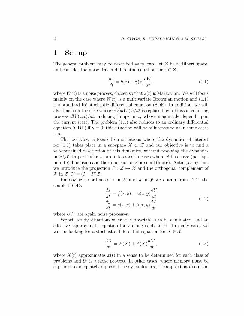
where W (t) is a noise process, chosen so that z(t) is Markovian. We will focusmainly on the case where W (t) is a multivariate Brownian motion and (1.1)is a standard Ito stochastic differential equation (SDE). In addition, we willalso touch on the case where γ(z)dW (t)/dt is replaced by a Poisson countingprocess dW (z, t)/dt, inducing jumps in z, whose magnitude depend uponthe current state. The problem (1.1) also reduces to an ordinary differentialequation (ODE) if γ ≡ 0; this situation will be of interest to us in some casestoo.

This overview is focused on situations where the dynamics of interestfor (1.1) takes place in a subspace X ⊂ Z and our objective is to find aself-contained description of this dynamics, without resolving the dynamicsin Z\X . In particular we are interested in cases where Z has large (perhapsinfinite) dimension and the dimension of X is small (finite). Anticipating this,we introduce the projection P : Z 7→ X and the orthogonal complement ofX in Z, Y = (I − P )Z.

Employing co-ordinates x in X and y in Y we obtain from (1.1) thecoupled SDEs

dx

dt= f(x, y) + α(x, y)

dU

dtdy

dt= g(x, y) + β(x, y)

dV

dt

(1.2)

where U ,V are again noise processes.We will study situations where the y variable can be eliminated, and an

effective, approximate equation for x alone is obtained. In many cases wewill be looking for a stochastic differential equation for X ∈ X :

dX

dt= F (X) + A(X)

dU ′

dt, (1.3)

where X(t) approximates x(t) in a sense to be determined for each class ofproblems and U ′ is a noise process. In other cases, where memory must becaptured to adequately represent the dynamics in x, the approximate solution

Extracting macroscopic dynamics: model problems & algorithms 3

X(t) is a component of a problem which evolves in a space of dimension higherthan the dimension of X , but still smaller than the dimension of Z. Weconsider cases where the original model (1.1) for z is either an autonomousODE or a noise-driven differential equation, such as an SDE, and wherethe effective dynamics (1.3) for X is either an ODE or an SDE. The ideaswe describe have discrete time analogues, and some of the algorithms weoverview extract a discrete time model in X , such as a Markov chain, ratherthan a continuous time model. We will also examine situations where theeffective dimension reduction can be carried out in the space of probabilitydensities propagated by paths of (1.1); this requires consideration of theMaster Equation for probability densities.

The primary motivation for this paper is to overview the wealth of recentwork concerning algorithms which attempt to find the effective dynamics inX . This work is, at present, not very unified and our aim is to highlightthe similarities and differences among the approaches currently emerging. Inorder to do this we will spend a substantial fraction of the paper explain-ing situations in which it is possible to find closed equations for X whichadequately approximate the dynamics of x ∈ X . Thus most of the paperwill be devoted to the development of model problems, and the underlyingtheoretical context in which they lie. Model problems are of primary impor-tance in order to make clear statements about the situations in which weexpect given algorithms to be of use, and in order to develop examples whichcan be used to test these algorithms. We do not state theorems and giveproofs— we present the essential ideas and reference the literature for detailsand rigorous analysis.

Section 2 contains an introduction to the Master Equation, first for count-able state space Markov chains. On uncountable state spaces, and for W (t)Brownian motion in (1.1), the Master Equation is a partial differential equa-tion (PDE)—the Fokker-Planck equation—and its adjoint—the Chapman-Kolmogorov equation—propagates expectations; we describe these PDEs. InSection 3 we outline the Mori-Zwanzig projection operator approach whichdescribes the elimination of variables at the level of the Master Equation.Sections 4–8 describe a variety of situations where an effective equation forthe dynamics in X can be derived. Section 9 is devoted to a description ofa variety of algorithms recently developed, or currently under development,which aim to find effective dynamics in X , given the full evolution equation(1.1) in Z.

The following provides an overview of a number of important themes


running throughout this paper.

i) Reduction Principles. In conceptualizing these algorithms it is impor-tant to appreciate that any algorithm aimed at extracting dynamics inX , given the equations of motion (1.1) in Z, has two essential com-ponents: (i) determining the projection P which defines X throughX = PZ; (ii) determining the effective dynamics in X . In some in-stances P is known a priori from the form of the model (1.1) and/orfrom physical considerations; in others its determination may be themost taxing part of the algorithm.

ii) Memory. An important aim of any such algorithm is to choose Pin such a way that the dynamics in X is memoryless. In principle,y can always be eliminated from (1.2) to obtain an equation for xalone but, in general, this equation will involve the past history of x;this is the idea of Mori-Zwanzig formalism. In order to understandand improve algorithms it is therefore important to build up intuitionabout situations in which memory in X disappears or, alternatively,in which it can be modelled by a few degrees of freedom. Sections 4-8 are all devoted to situations where the effect of memory disappearscompletely, except Section 7 which also describes situations where amemory effect remains, but can be modelled by adding a small numberof extra degrees of freedom.

iii) Classification of Model Problems. It is useful to classify the modelproblems according to whether or not the dynamics in Z and X aredeterministic or stochastic. The situations outlined in Sections 4, 5, 6,7, 8 are of the form D-D, D-D, S-S, D-S and S-D respectively where Ddenotes Deterministic, and S denotes Stochastic, and the first (resp. sec-ond) letter defines the type of dynamics in Z (resp. X ).

iv) Scale Separation. Sections 4 – 6 all rely on explicit time-scale separationto achieve the memoryless effect. In contrast the examples in Section 7rely on the high dimensionality of Y relative to X ; the mean time-scalein Y then separates from that in X , but there is no pure separation ofscales. Thus, whilst scale separation is a useful concept which unifiesmany of the underlying theoretical models in this subject area, thedetails of how one establishes rigorously a given dimension reduction


differ substantially depending on whether there is a clear separation ofscales, or instead a separation in a mean sense.

2 The Master Equation

In this section we consider dynamical systems of the form (1.1) within aprobabilistic setting, by considering the evolution of probability measuresinduced by the dynamics of paths of (1.1). There are two essential reasonsfor considering a probabilistic description rather than a pathwise one:

i) Variable reduction is often related to uncertainty in initial data, hencewith ensembles of solutions. The reduced initial data x(0) = Pz(0)are a priori compatible with a large set of initial data z(0) for the fullevolution equation. Every initial datum z(0) gives rise to a differentsolution z(t) and to different projected dynamics x(t). In many cases itis meaningless to consider how x(0) evolves into x(t) without specifyinghow the eliminated variables, y(0), are initially distributed.

ii) The evolution of the measure is governed by a linear PDE. In spiteof the increased complexity due to the infinite dimensionality of thesystem, the linearity enables the use of numerous techniques adaptedfor linear systems, such as projection methods, and perturbation ex-pansions.

A useful example illustrating the first point comes from statistical me-chanics. It is natural to specify the temperature in (some components of)a molecular system, since it is a measurable macroscopic quantity, withoutspecifying the exact positions and velocities; this corresponds to specifying aprobability measure on the positions and velocities, with variance determinedby the temperature.

A useful example illustrating the second point is passive tracer advec-tion: the position of a particle advected in a velocity field, and subject tomolecular diffusion, can then be modelled by a nonlinear SDE; collectionsof such particles have density satisfying a linear advection-diffusion equa-tion. In the absence of noise this simply reflects the fact that the method ofcharacteristics for a linear hyperbolic problem gives rise to nonlinear ODEs.

In Subsection 2.1 we describe the derivation of the equation governingprobability measures for countable state space Markov chains; in Subsection


2.2 we generalize this to the case of Ito SDEs, which give rise to Markovprocesses on uncountable state spaces.

2.1 Countable State Space

Consider a continuous time Markov chain z(t), t ≥ 0, taking values in thestate space I ⊆ {0, 1, 2, . . . }. Let pij(t) be the transition probability fromstate i to j:

pij(t) = P{z(t) = j | z(0) = i},i.e., the probability that the process is in state j at time t, given that it wasin state i at time zero. The Markov property implies that for all t,∆t ≥ 0,

pij(t+ ∆t) =∑

k

pik(t)pkj(∆t),

and sopij(t+ ∆t)− pij(t)

∆t=

∑k

pik(t)`kj(∆t),

where

`kj(∆t) =1

∆t×

{pkj(∆t) k 6= j

pjj(∆t)− 1 k = j

Suppose that the limit `kj = lim∆t→0 `kj(∆t) exists. We then obtain, for-mally,

dpij

dt=

∑k

pik`kj. (2.1)

Because∑

j pij = 1 it follows that∑

j ìj(∆t) = 0, and we expect that∑j

ìj = 0.

Introducing the matrices P , L with entries pij, ìj, respectively, i, j ∈ I,equation (2.1) reads, in matrix notation,

dP

dt= PL, P (0) = I. (2.2)

Since P (t) = exp(Lt) solves this problem we see that P and L commute sothat P (t) also solves

dP

dt= LP, P (0) = I. (2.3)


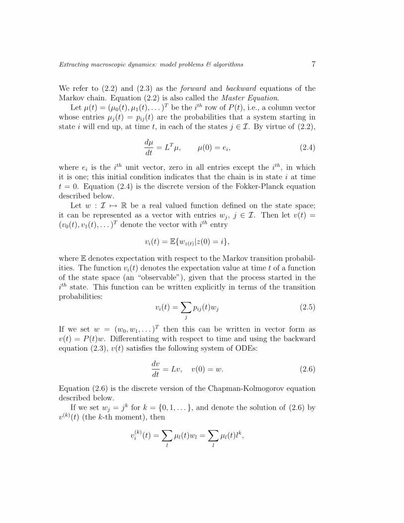
We refer to (2.2) and (2.3) as the forward and backward equations of theMarkov chain. Equation (2.2) is also called the Master Equation.

Let µ(t) = (µ0(t), µ1(t), . . . )T be the ith row of P (t), i.e., a column vector

whose entries µj(t) = pij(t) are the probabilities that a system starting instate i will end up, at time t, in each of the states j ∈ I. By virtue of (2.2),

dµ

dt= LTµ, µ(0) = ei, (2.4)

where ei is the ith unit vector, zero in all entries except the ith, in whichit is one; this initial condition indicates that the chain is in state i at timet = 0. Equation (2.4) is the discrete version of the Fokker-Planck equationdescribed below.

Let w : I 7→ R be a real valued function defined on the state space;it can be represented as a vector with entries wj, j ∈ I. Then let v(t) =(v0(t), v1(t), . . . )

T denote the vector with ith entry

vi(t) = E{wz(t)|z(0) = i},

where E denotes expectation with respect to the Markov transition probabil-ities. The function vi(t) denotes the expectation value at time t of a functionof the state space (an “observable”), given that the process started in theith state. This function can be written explicitly in terms of the transitionprobabilities:

vi(t) =∑

j

pij(t)wj (2.5)

If we set w = (w0, w1, . . . )T then this can be written in vector form as

v(t) = P (t)w. Differentiating with respect to time and using the backwardequation (2.3), v(t) satisfies the following system of ODEs:

dv

dt= Lv, v(0) = w. (2.6)

Equation (2.6) is the discrete version of the Chapman-Kolmogorov equationdescribed below.

If we set wj = jk for k = {0, 1, . . . }, and denote the solution of (2.6) byv(k)(t) (the k-th moment), then

v(k)i (t) =

∑l

µl(t)wl =∑

l

µl(t)lk,


where µ(t) is defined as above. Notice that, if the evolution is deterministic,then µ(t) will remain at all times a unit vector, em(t), for some fixed integerm. Then

v(k)i (t) = [v

(1)i (t)]k,

so that the first moment characterizes the process completely. This ideageneralizes to continuous state space processes, for example those in thenext subsection.

This suggests a more a general question: for a given Markov chain on Istarting in state i, do there exist a small number of linear functions of p(t)(i.e., expectation values of functions on I) which, at least approximately,characterize the behaviour of (some) components of the process? This ques-tion is at the heart of the model problems and algorithms that we studyhere.

Some of the algorithms we highlight work in discrete time. Then theanalogue of (2.4) is the iteration

µn+1 = Tµn, µ0 = ei.

Again, if the state space I is large or infinite, it is natural to ask whetherthe expectation values of a small number of functions of the process can beused to approximate the whole process, or certain aspects of its behaviour.

2.2 Fokker-Planck and Chapman-Kolmogorov Equa-tions

The concepts introduced in Subsection 2.1 are now extended to continuoustime Markov processes over uncountable state spaces, specifically, to diffu-sion processes defined by SDEs. Consider the case where W (t) is a multi-dimensional Brownian motion and (1.1) is an Ito SDE. We assume that Zhas dimension d and let ∇ and ∇· denote gradient and divergence in Rd. Thegradient can act on both scalar valued functions φ, or vector valued functionsv, via

∇φ =∂φ

∂zi

ei, ∇v =∂vi

∂zj

eieTj


for orthonormal basis {ei} in Rd. The divergence acts on vector valuedfunctions v, or matrix valued functions A via

∇ · v =∂vi

∂zi

, ∇ · A =∂Aij

∂zj

ei.

In the preceding we are assuming the Einstein summation convention, wherebyrepeated indices imply a summation. Below we will use ∇x (resp. ∇y) todenote gradient or divergence with respect to x (resp. y) co-ordinates alone.

With the functions h(z),γ(z) defining the SDE (1.1) we define

Γ(z) = γ(z)γ(z)T ,

and then the generator L by

Lφ = h · ∇φ+1

2Γ : ∇(∇φ), (2.7)

where · denotes the standard inner-product on Rd, and : denotes the innerproduct on Rd×d which induces the Frobenius norm—A : B = trace(ATB).We will also be interested in the operator L∗ defined by

L∗ρ = −∇ · (hρ) +1

2∇ · [∇ · (Γρ)] ,

which is the adjoint of L with respect to the scalar product

〈φ, ρ〉 =

∫Zφ(z)ρ(z) dz,

i.e., 〈Lφ, ρ〉 = 〈φ,L∗ρ〉.If we consider solutions of (1.1) with initial data distributed according to

a measure with density ρ0(z) then, at time t > 0, z(t) is distributed accordingto a measure with density ρ(z, t) satisfying the Fokker-Plank equation

∂ρ

∂t= L∗ρ (z, t) ∈ Rd × (0,∞),

ρ = ρ0 (z, t) ∈ Rd × {0} .(2.8)

This is the analogue of the Master Equation (2.4) in the countable state spacecase. We are implicitly assuming that the measure µt, defined by µt(A) =P{z(t) ∈ A}, has density ρ(z, t) with respect to Lebesgue measure. Here P


is the probability measure on paths of Brownian motion (Wiener measure),and we denote by E expectation with respect to this measure. Whether ornot such a smooth density exists depends on the (hypo-) ellipticity propertiesof L.

The adjoint counterpart of the Fokker-Planck equation is the Chapman-Kolmogorov equation. Let w(z) be a function on Z and consider the functionv(z0, t) = E[w(z(t))|z(0) = z0], where the expectation is with respect toall Brownian driving paths satisfying z(0) = z0. Then v(z, t) solves theChapman-Kolmogorov equation

∂v

∂t= Lv (z, t) ∈ Rd × (0,∞),

v = w (z, t) ∈ Rd × {0} .(2.9)

This is the analogue of (2.6) in the countable state space case. If γ ≡ 0 in(1.1), i.e. the dynamics are deterministic, and ϕt is the flow on Z so thatz(t) = ϕt(z(0)), then the Chapman-Kolmogorov equation (2.9) reduces toa hyperbolic equation, whose characteristics are the integral curves of theODE (1.1), and its solution is v(z, t) = w(ϕt(z)).

We will adopt the semigroup notation, denoting the solution of (2.8) byρ(z, t) = eL

∗tρ0(z), and the solution of (2.9) by v(z, t) = eLtw(z). Theconnection between the two evolution operators is as follows:

eLtw(y) =

∫Z(eL

∗tρ0)(z)w(z) dz, (2.10)

where ρ0(z) = δ(z − y). This is the analogue of (2.5) in the countable statespace case. Indeed, both sides of (2.10) represent the expectation value attime t of w(z(t)) with respect to the distribution of trajectories that originateat the point y.

2.3 Discussion and Bibliography

A good background reference on Markov chains is Norris [Nor97]. For adiscussion of SDEs from the Fokker-Planck viewpoint, see Risken [Ris84] orGikhman and Skorokhod [GS96] . For a discussion of the generator L, andthe Chapman Kolmogorov equation, see Oksendal [Øks98]. For a discussionconcerning ellipticity, hypo-ellipticity and smoothness of solutions to theseequations see Rogers and Williams [RW00].


3 Mori-Zwanzig Projection Operators

The Mori-Zwanzig formalism is a technique developed for irreversible statis-tical mechanics to reduce, at least formally, the dimensionality of a systemof ODEs. For a system of the form (1.2), with α = β ≡ 0, the Mori-Zwanzigformalism yields an equation for x(t) of the form

dx(t)

dt= f(x(t)) +

∫ t

0

K(x(t− s), s) ds+ n(x(0), y(0), t). (3.1)

The first term on the right hand side is only a function of of the instantaneousvalue of x at time t, and therefore represents a “Markovian” term. The secondterms depends on values of x at all times between 0 and t, and thereforerepresents a “memory” effect. The function K : X × [0,∞) 7→ X is thememory kernel. The function n(x(0), y(0), t) satisfies an auxiliary equation,known as the orthogonal dynamics equation, and depends on full knowledge ofthe initial conditions. If the initial data for y(0) is random then this becomesa random force. The Mori-Zwanzig formalism is a nonlinear extension of themethod of undetermined coefficients for variable reduction in linear systems.

The reduction from (1.2) to an equation of the form (3.1) is not unique.It relies on the definition of an operator P, the projection1, which mapsfunctions of (x, y) into functions of x only. The projection operator that ismost appropriate in our context is the following. The state of the systemis viewed as random, distributed with a probability density ρ(x, y). Anyfunction w(x, y) has then an expected value, which we denote by Ew; theexpected value is the best approximation of a function by a constant in an L2

sense. If the value of the coordinate x is known, then the best approximationto w(x, y) is the conditional expectation of w given x, usually denoted byE[w|x]. The conditional expectation defines a mapping w 7→ Pw = E[w|x]from functions of (x, y) to functions of x. Specifically,

(Pw)(x) =

∫Y ρ(x, y)w(x, y) dy∫

Y ρ(x, y) dy.

With the initial value y(0) viewed as random, the function n(x(0), y(0), t)is a random function, or a stochastic process. The equation (3.1) is derivedsuch that n(x(0), y(0), t) has zero expected value for all times, which makes

1Not to be confused with the projection P defined in the Introduction


it an unbiased “noise”. In the original context of statistical mechanics, wherethe governing dynamics are Hamiltonian, the noise n(x(0), y(0), t) and thememory K(x, t) satisfy what is known as the fluctuation-dissipation relation.Equation (3.1) is often called a generalized Langevin equation. Analogouslyto the Fokker-Planck versus Chapman-Kolmogorov duality there exist twoversions of the Mori-Zwanzig formalism: one for the expectation value offunctions and one for probability densities.

The derivation of (3.1) is quite abstract, and we only present here asummary. If ϕt(x, y) is the flow map induced by (1.2) with α = β = 0, andP is the projection (x, y) 7→ x, then the function x(t) is more accuratelywritten as Pϕt(x, y), where here (x, y) are the initial data. The x-equationin (1.2) is

∂

∂tPϕt(x, y) = f(ϕt(x, y)), (3.2)

and, of course, is not a closed equation for Pϕt(x, y).The first step in the Mori-Zwanzig formalism is to replace f on the right

hand side by its best approximation given only its first argument. Thus (3.2)is rewritten as follows:

∂

∂tPϕt(x, y) = (Pf)(Pϕt(x, y)) +

[f(ϕt(x, y))− (Pf)(Pϕt(x, y))

]. (3.3)

The function Pf is identified with f in (3.1).The next stage is to re-arrange the terms in the square brackets in (3.3).

Defining the operator L = f(x, y) · ∇x + g(x, y) · ∇y, the noise functionn(x, y, t) is defined as the solution of the orthogonal dynamics equation:

∂n

∂t= (I −P)Ln

n(x, y, 0) = f(x, y)− (Pf)(x).(3.4)

The memory kernel is defined as

K(x, t) = PLn(x, y, t).

One can then check explicitly that the residual terms in (3.3) can be writtenas

f(ϕt(x, y))− (Pf)(Pϕt(x, y)) = n(x, y, t) +

∫ t

0

K(Pϕt−s(x, y), s) ds, (3.5)


hence (3.3) takes the form (3.1).To understand the last identity, we note that the left hand side can be

written asetL(I −P)Lw,

where w = w(z) = Pz, hence Lw(z) = f(z); semi-group notation hasbeen used for the solution operator of the flow map ϕt(z): exp(tL)w(z) =w(ϕt(z)). The noise can, likewise, be written in the form n(z, t) = exp[t(I −P)L] (I −P)Lw, so that the right-hand side of (3.5) reads

εt(I−P)L (I −P)Lw +

∫ t

0

e(t−s)LPLes(I−P)L (I −P)Lw ds.

The validity of (3.5) is a consequence of the operator identity,

etL = et(I−P)L +

∫ t

0

e(t−s)LPLes(I−P)L ds,

known in the Physics literature as Dyson’s formula [EM90].It is important to point out that (3.1) is not simpler than the original

problem. The complexity has been transfered, in part, to the solution ofthe orthogonal dynamics (3.4). The value of (3.1) is first conceptual, andsecond that it constitutes a good starting point for asymptotic analysis andstochastic modelling. In particular it suggests that deterministic problemswith random data may be modelled by stochastic problems with memory. Inthe case where the memory can be well-approximated by the introductionof a small number of extra variables and so that the whole system is thenMarkovian in time, this leads to a simple low dimensional stochastic modelfor the dynamics in X . This basic notion underlies many of the examplesused in the following.


The original derivation of Mori-Zwanzig formalism can be found in Mori[Mor65] and Zwanzig [Zwa73]. Most of the statistical physics literature usesthe Mori Zwanzig formalism with a projection on the span of linear functionsof the essential degrees of freedom. Zwanzig in [Zwa80] developed a nonlineargeneralization, which is equivalent to the conditional expectation used here.All the above references use the “Chapman-Kolmogorov” version of this for-malism; the “Fokker-Planck” version can be found in [MFS74]. The existence


of solutions to the orthogonal dynamics equation (3.4) turns out to be verysubtle; see Givon et al. [GHK03]. An alternative to the Mori-Zwanzig ap-proach is to derive convolutionless, non-Markovian evolution equations; thisapproach, and an application in plasma physics, is outlined in [VEG98] anda more recent applications in [KMVE03]. Recent uses of the Mori-Zwanzigformalism in the context of variable reduction can be found in Just et al.[JKRH01, JGB+03] and Chorin et al. [CHK02].

4 Scale Separation and Invariant Manifolds

In the classification of Section 1, this section is devoted to problems of thetype D-D – deterministic systems with lower dimensional deterministic sys-tems embedded within them. The key mathematical construct used is thatof invariant manifolds, and scale separation is the mechanism by which thesemay be constructed. For such problems the initial conditions in Y are irrel-evant, after, perhaps, an initial transient.

4.1 Theory

Consider equations (1.2) in the deterministic setting when α, β ≡ 0 and letf(x, y) and g(x, y) be written in the following form:

f(x, y) = L1x+ f(x, y),

g(x, y) = L2y + g(x, y).(4.1)

Assume for simplicity that the operators L1, L2 are self-adjoint and that themaximum eigenvalue of L2 is less than the minimum of L1. If the gap in thespectra of L1 and L2 is large then for the purely linear problem, found bydropping f and g, the dynamics is dominated, relatively speaking, by thedynamics in X . In the fully nonlinear problem, if the gap is assumed largerelative to the size of f and g (and the argument can be localized by useof cut-off functions), then the existence of an exponentially attractive andinvariant manifold

y = η(x)


may be proved. Thus, after an initial transient, the effective dynamics in Xis governed by the approximating equation

dX

dt= L1X + f(X, η(X))

X(0) = x(0).(4.2)

Specifically, under suitable conditions on the spectra of L1 and L2, X(t) andx(t) remain close, at least on bounded time intervals. In many cases, thevalidity of this approximation requires assumptions on the initial value ofthe discarded variables y(0).

4.2 Model Problem

A useful model problem arises when X = Rn, Y = R and (1.2) has the form,for ε� 1,

dx

dt= f(x, y)

dy

dt= −y

ε+g(x)

ε.

(4.3)

In reference to the spectral properties of L1, L2 in (4.1), the unique eigenvalueof L2 is −1/ε, which for small enough ε is less than the minimum eigenvalueof the linear component of f(x, y).

Assume that f , g are smooth and bounded, with all derivatives bounded.Then, seeking an approximate invariant manifold in the form

y = g(x) + εg1(x) +O(ε2)

gives, substituting into the y-equation in (4.3), expanding to O(1) and usingthe x-equation in (4.3),

∇g(x) · f(x, g(x)) = −g1(x).

Thus, up to errors of O(ε2), the reduced dynamics are

dX

dt=f(X,G(X)), (4.4)

G(X) =g(X)− ε∇g(X) · f(X, g(X))), (4.5)

with X(0) = x(0). Note that for the derivation to be consistent the initialvalue y(0) should be close to the invariant manifold, |y(0)− g(x(0))| = O(ε),


otherwise, an initial layer forms near time t = 0; after this initial layer theinitial condition in Y is essentially forgotten.

Example 4.1 Consider the equations

dx1

dt= −x2 − x3

dx2

dt= x1 +

1

5x2

dx3

dt=

1

5+ y − 5x3

dy

dt= −y

ε+x1x3

ε,

(4.6)

so that X = R3 and Y = R. The expression (4.5) with ε = 0 indicates that,for small ε, y ≈ x1x3, so that the solution for x = (x1, x2, x3) should be wellapproximated by X = (X1, X2, X3) solving the Rossler system [Ros76]

dX1

dt= −X2 −X3

dX2

dt= X1 +

1

5X2

dX3

dt=

1

5+X3(X1 − 5)

(4.7)

Figure 4.1 shows the attractor for (x, y), projected onto (x1, x2), comparedwith the attractor forX projected onto (X1, X2) at the value ε = 0.01. Noticethe clear similarities between the two. Figure 4.2 compares the histogramsfor x1 and X1 over 105 time units; the two histograms are clearly closelyrelated.


The reduction of differential systems with attracting slow manifold intodifferential-algebraic systems is due originally to independent work of Levin-son and Tikhonov (O’Malley [O’M91], Tikhonov et al. [TVS85]). The use ofa spectral gap sufficiently large relative to the size of the nonlinear terms isused in the construction of local stable, unstable and center manifolds (e.g.,Wiggins [Wig90]), slow manifolds (Kreiss [Kre92]) and inertial manifolds


−8 −6 −4 −2 0 2 4 6 8 10−10

−8

−6

−4

−2

0

2

4

6

8Atrractor. ε=0.01

x1

x 2

−8 −6 −4 −2 0 2 4 6 8 10−10

−8

−6

−4

−2

0

2

4

6

8Attractor.

X1

X2

Figure 4.1: Comparison between the attracting sets for (4.6) with ε = 0.01(left) and (4.7) (right), projected on the (x1, x2) and (X1, X2) planes, respec-tively.

−10 −5 0 5 10 150

0.01

0.02

0.03

0.04

0.05

0.06

0.07

0.08

0.09

0.1ε = 0.01

x1 X

1

Em

piric

al M

easu

re

Figure 4.2: Comparison between the empirical measures of x1 solving (4.6)with ε = 0.01 (solid line), and X1 solving (4.7) (dashed line). The empiricalmeasure was computed from a trajectory over a time interval of 105 units.


(Constantin et al. [CFNT94]). A variety of methods of proof exist, pre-dominantly the Lyapunov-Perron approach (Hale [Hal88], Temam [Tem99])and the Hadamard graph transform (Wells [Wel76]). The numerical calcula-tion of slow dynamics, via dimension reduction in fast-slow systems and withapplication to problems in chemical kinetics, is described in [DH96].

5 Scale Separation and Averaging

There exists a vast literature on systems, which in the classification of Sec-tion 1 are of type D-D, that can be unified under the title of “averagingmethods”. Averaging methods have their early roots in celestial mechanics,but apply to a broad range of applications.

Averaging methods are concerned with situations where, for fixed x, thetrajectories of the y-dynamics do not tend to a fixed point. Instead, thefast dynamics affect the slow dynamics through the empirical measure thatits trajectories induce on Y . The simplest such situation is where the fastdynamics converge to a periodic solution; other possibilities are convergenceto quasi-periodic solutions, or chaotic solutions.

5.1 The averaging method

For concreteness, we limit our discussion to systems with scale separation ofthe form

dx

dt= f(x, y)

dy

dt=

1

εg(x, y),

(5.1)

where ε� 1.

The starting point is to analyze the behaviour of the fast dynamics withx being a parameter. In the previous section we considered systems in whichthe fast dynamics converge to an x-dependent fixed point. This gives rise toa situation where the y variables are “slaved” to the x variables. Averaginggeneralizes this idea to situations where the dynamics in the y variable, withx fixed, is more complex.

We start by discussing the case when the dynamics for y is ergodic. Ageneral theorem on averaging, due to Anosov, applies in this case. Let ϕt

x(y)


be the solution operator of the fast dynamics with x a fixed parameter. Then

d

dtϕt

x(y) = g(x, ϕtx(y)), ϕ0

x(y) = y (5.2)

(the 1/ε rate factor has been omitted because time can be rescaled when thefast dynamics is considered alone). The fast dynamics is said to be ergodic,for given fixed x, if for all functions ψ : Y → R the limit of the time average

limT→∞

1

T

∫ T

0

ψ(ϕtx(y)) dt,

exists and is independent of y. In particular, ergodic dynamics define anergodic measure, µx, on Y , which is invariant under the fast dynamics; notethat the invariant measure depends, in general, on x.

Anosov’s theorem states that, under ergodicity in Y for fixed x, the slowvariables x(t) converge uniformly on any bounded time interval to the solu-tion X(t) of the averaged equation,

dX

dt= F (X) (5.3)

F (ζ) =

∫Yf(ζ, y)µζ(dy). (5.4)

Similar ideas prevail if the invariant measure generated by the y dynamicsdepends upon the initial data in Y , but are complex to state in general. Weoutline some of these situations in the remainder of this section.

5.2 Model Problem

An application area where averaging techniques are of current interest ismolecular dynamics. Here one encounters Hamiltonian systems with strongpotential forces, responsible for fast, small amplitude, oscillations arounda constraining sub-manifold. The goal is to describe the evolution of theslowly evolving degrees of freedom by averaging over the rapidly oscillatingvariables. Bornemann and Schutte [BS97] developed a systematic treatmentof such systems that builds upon earlier work by Rubin and Ungar [RU57],using the techniques of time-homogenization [Bor98].

The general setting is a Hamiltonian of the form

H(z, p) =∑

j

p2j

2mj

+ V (z) +1

ε2U(z),


where z = (z1, . . . , zn+m) and p = (p1, . . . , pn+m) are the coordinates and mo-menta, V (z) is a “soft” potential, whereas ε−2U(z) is a “stiff” potential. It isassumed that U(z) attains a global minimum, 0, on a smooth n-dimensionalmanifold, M. The limiting behaviour of the system, as ε→ 0, depends cru-cially on the choice of initial conditions. The setting appropriate to molecularsystems is where the total energy E (which is conserved) is assumed inde-pendent of ε. Then, as ε → 0, the states of the system are restricted to anarrow band in the vicinity of M; the goal is to approximate the evolutionof the system by a flow on M.

Example 5.1 The following simple example, taken from [BS97], shows howproblems with this form of Hamiltonian can be cast in the general set-up ofequations (5.1). Consider a two-particle system with Hamiltonian,

H(x, p, y, v) =1

2(p2 + v2) + V (x) +

ω(x)

2 ε2y2,

where (x, y) and (p, v) are the respective coordinates and momenta of the twoparticles, V (x) is a non-negative potential and ω(x) is assumed to be uni-formly bounded away from zero: ω(x) ≥ ω > 0 for all x. The correspondingequations of motion are

dx

dt= p

dp

dt= −V ′(x)− ω′(x)

2ε2y2

dy

dt= v

dv

dt= −ω(x)

ε2y.

The assumption that the energy does not depend on ε implies that y2 ≤2ε2E/ω and the solution approaches the submanifold y = 0 as ε → 0. Note,however, that y appears in the combination y/ε in the x equations. Thus itis natural to make the change variables η = y/ε. The equations then read

dx

dt= p

dp

dt= −V ′(x)− ω′(x)

2η2

dη

dt=

1

εv

dv

dt= −ω(x)

εη.

In these variables we recover a system of the form (5.1) with “slow” variables,(x, p), and “fast” variables, (η, v). The fast equations represent an harmonicoscillator whose frequency, ω1/2(x), is modulated by the x variables.


The limiting solution of a fast modulated oscillator can be derived usinga WKB expansion [BO99], but it is more instructive to consider the followingheuristic approach. Suppose that the slow variables (x, p) are given. Then,the energy available for the fast variables is

Hη(x, p) = E − 1

2p2 − V (x).

Harmonic oscillators satisfy an equi-partition property, whereby, on average,the energy is equally distributed between its kinetic and potential contribu-tions (the virial theorem). Thus the time-average of the kinetic energy of thefast oscillator is ⟨

ω(x)

2η2

⟩=

1

2

[E − 1

2p2 − V (x)

],

where (x, p) are viewed as fixed parameters and the total energy E is specifiedby the initial data. The averaging principle states that the rapidly varyingη2 in the equation for p can be approximated by its time-average, giving riseto a closed system of equations for (X,P ) ≈ (x, p),

dX

dt= P

dP

dt= −V ′(X)− ω′(X)

2ω(X)

[E − 1

2P 2 − V (X)

],

(5.5)

with initial data E, X0 = x0 and P0 = p0. It is easily verified that (X,P )satisfying (5.5) conserve the following invariant,

1

ω(X)

[E − 1

2P 2 − V (X)

],

Thus, (5.5) reduces to the simpler form

dX

dt= P

dP

dt= −V ′(X)− c ω′(X),

where

c =1

2ω(X0)

[E − 1

2P 2

0 − V (X0)

].


This means that the influence of the stiff potential on the slow variables isto replace the potential V (x) by an effective potential,

V eff(x) = V (x) + c ω(x).

Note that the limiting equation contains memory of the initial conditions forthe fast variables, through the initial energy E. Thus the situation differsslightly from the Anosov theorem described previously.

This heuristic derivation is made rigorous in [BS97], using time-homogenizationtechniques, and it is also generalized to higher dimension. The conditionthat ω(x) be bounded away from zero may be viewed as a non-resonancecondition. Resonances become increasingly important as the co-dimension,m, increases, limiting the applicability of the time-homogenization approach(Takens [Tak80]).


A detailed account on the averaging method, as well as numerous examplescan be found in Sanders and Verhulst [SV85]. Much of the literature on av-eraging was published in Russian and has remained untranslated; an Englishreview of this literature is found in Lochak and Meunier [LM88].

Anosov’s theorem requires the fast dynamics to be ergodic. Often ergod-icity fails due to the presence of “resonant zones”—regions in X for which thefast dynamics is not ergodic. Arnold and Neistadt [LM88] extended Anosov’sresult for situations in which the ergodicity assumption fails on a sufficientlysmall set of x ∈ X .

The situations in which the fast dynamics tend to fixed points, periodicsolutions, or chaotic solutions can be treated in a unified manner throughthe introduction of Young measures. Artstein and co-workers considered aclass of singularly perturbed system of type (5.1), with attention given to thelimiting behaviour of both slow and fast variables. In all of the above casesthe pair (x, y) can be shown to converge to (X,µX), where X is the solutionof

dX

dt=

∫Yf(X, y)µX(dy),

and µX is the ergodic measure on Y ; the convergence of y to µX is in thesense of Young measure. (In the case of a fixed point the Young measure isconcentrated at a point.) A general theorem along these lines is proved in[Art02].


There are many generalization to this idea. The case of non-autonomousfast dynamics, as well as a case with infinite dimension are covered in [AS01].Moreover, these results still make sense even if there is no unique invariantmeasure µx, in which case the slow variables can be proved to satisfy a (non-deterministic) differential inclusion [AV96].

In the context of stochastic systems, an interesting set-up for averagingis to consider systems of the form

dx

dt= f(x, y)

dy

dt=

1

εg(x, y) +

1√ε

dV

dt.

(5.6)

If the y dynamics, with x frozen at ζ, is ergodic, then the analogue of theAnosov result holds with µζ the invariant measure of this y dynamics. Thisgives rise to a set-up of type S−D. This idea is generalized in Subsection 6.1where the chosen scaling leads not only to an averaged deterministic vectorfield in x, but also to additional stochastic fluctuations.

6 Scale Separation and White Noise Approx-

imation

In Section 4 a separation of time-scales led to deterministic dynamics in Xand the “slaving” of the y variable to the x variable. In the Fokker-Planckpicture this corresponds to a situation where, after a short transient, theprobability density has the approximate form

ρ(x, y, t) ≈ δ(y − η(x))ρ(x, t)

(the measure is concentrated near the approximation to the invariant mani-fold, namely y = η(x)).

In this section we consider how to use the PDEs for propagation of ex-pectations and probability densities to study stochastic dimension reductionwhen there is a clear scale separation between the x and y dynamics, butthe effective dynamics in X is stochastic; the original dynamics in Z may bedeterministic or stochastic. Thus we study problems of the form D-S or S-Sin the classification of Section 1. The theory will be developed for problemswith a skew-product structure: the dynamics for y evolves independently of


the dynamics for x. This simplifies the analysis, but is not necessary; inthe final subsection we review literature when full back-coupling between thevariables is present.

In the skew-product case we will look for an approximate probabilitydensity of the form

ρ(x, y, t) ≈ ρ∞(y)ρ(x, t),

with ρ∞(·) a smooth probability density on Y , invariant under the y-dynamics.This ansatz assumes that the distribution of y reaches equilibrium on a timescale much shorter than the time scale over which x evolves. This is theprobabilistic analog of the slaving and averaging techniques of the previoustwo sections. When full back-coupling is present, the approximate solutionwill take the form

ρ(x, y, t) ≈ ρ∞(x, y)ρ(x, t), (6.1)

where ρ∞(x, y) is a density invariant under the y-dynamics, with x viewedas a fixed parameter.

We start by studying the approach based on the Chapman-Kolmogorovpicture and then re-study the problem using the Fokker-Planck approach.The two approaches are both illustrated by a model problem, accompanied bynumerical results. The final subsection overviews the literature and describesa variety of extensions of the basic idea.

6.1 Chapman-Kolmogorov Picture

Consider the case of (1.2) where α ≡ 0 and f, g, β are of the form

f(x, y) =1

εf0(x, y) + f1(x, y)

g(x, y) =1

ε2g0(y)

β(x, y) =1

εβ0(y),

(6.2)

that isdx

dt=

1

εf0(x, y) + f1(x, y)

dy

dt=

1

ε2g0(y) +

1

εβ0(y)

dV

dt.

Both the x and y equations contain fast dynamics, but the dynamics in y isan order of magnitude faster than x (note that white noise scales differently


from regular time derivatives and that, in the Fokker-Planck picture, thecontributions from both the drift term, g, and the diffusion term, β, are oforder 1/ε2). Then the variable y induces fluctuations in the equation for x,(which will see below are formally of order 1/ε). We are going to assume thatf0(x, y) averages to zero under the y dynamics, but that f1(x, y) does not. Incertain situations it can then be shown that both terms in f contribute at thesame order. The term f0 will give the effective stochastic contribution and f1

the effective drift. One way to see this is by using the Chapman-Kolmogorovequation and we now develop this idea. Although the underlying theory inthis area is developed by Kurtz [Kur73], we follow the recent presentationgiven by Majda et al. [MTVE01] in which the mathematical structure ismade very clear through perturbation expansions.

Recall that v(x, y, t) satisfying equation (2.9), namely

∂v

∂t= Lv, v(x, y, 0) = w(x, y),

is the expected value at time t of w(·) over all solutions starting at thepoint (x, y); the probability space is induced by the Brownian motion in they variables. If w is only a function of x, then v(x, y, t) (which remains afunction of both x and y) describes the expected evolution of a propertypertinent to the essential dynamics on X .

Substituting (6.2) into the Chapman-Kolmogorov equation (2.9) withw = w(x) gives,

∂v

∂t=

1

ε2L1v +

1

εL2v + L3v

v(x, y, 0) = w(x),(6.3)

where

L1v = g0 · ∇yv +1

2(β0β

T0 ) : ∇y(∇yv) (6.4)

L2v = f0 · ∇xv (6.5)

L3v = f1 · ∇xv. (6.6)

We seek an expansion for the solution with the form

v = v0 + εv1 + ε2v2 + · · ·


Substituting this expansion into (6.3) and equating powers of ε gives a hier-archy of equations, the first three of which are

L1v0 = 0 (6.7)

L1v1 = −L2v0 (6.8)

L1v2 =∂v0

∂t− L2v1 − L3v0. (6.9)

The initial conditions are that v0 = w and vi = 0 for i ≥ 1.Note that L1, given by (6.4), is the Chapman-Kolmogorov operator con-

strained to the y-dynamics, and that constants (in y) are in the null-spaceof L1. Assume that there is a unique density ρ∞(y) in the null-space of L∗1(i.e., a unique density invariant under the y-dynamics), and denote by 〈·〉averaging with respect to this density. Assume further that the dynamics isergodic in the sense that any initial density ρ0(y), including a Dirac mass,tends, as t→∞, to the unique invariant density ρ∞(y); the system “returnsto equilibrium”. By (2.10)

limt→∞

eL1tφ(y0) = limt→∞

∫Yφ(y)

(eL

∗1tρ0

)(y) dz =

∫Yφ(y)ρ∞(y) dy = 〈φ〉 ,

(6.10)where ρ0(y) = δ(y − y0) and the limit is attained for any y0. Later we willalso assume that the operator L1 is negative definite on the inner productspace weighted by the invariant density and excluding constants; this kindof spectral gap is characteristic of many ergodic systems.

We now argue that functions φ satisfying L1φ = 0 are independent of y.Indeed,

d

dseL1sφ(y) = eL1sL1φ(y) = 0,

so that φ(y) = eL1sφ(y) for all s. Letting s→∞ and using (6.10) we get

φ(y) = 〈φ〉 ,

and the latter is independent of y. Thus, the first equation (6.7) in thehierarchy implies v0 = v0(x, t).

Consider next the v1 equation (6.8). For it to be solvable, L2v0 has tobe orthogonal to the kernel of L∗1, which by assumption contains only ρ∞(y).Thus, orthogonality to the kernel of L∗1 amounts to averaging to zero under


the y-dynamics. The solvability condition is then 〈L2v0〉 = 0, or substituting(6.5):

〈f0〉 · ∇xv0(x, t) = 0.

Thus, for the expansion to be consistent it suffices that 〈f0〉 ≡ 0; this meansthat the leading order x dynamics averages to zero under the invariant mea-sure of the y dynamics. It follows that the equation for v1 is solvable and wemay formally write

v1 = −L−11 L2v0.

Similarly, considering (6.9) the solvability condition for v2 becomes

∂v0

∂t= −

⟨L2L−1

1 L2v0

⟩+ 〈L3v0〉 . (6.11)

In view of the fact that L2 and L3 are first order differential operators inx, that L1 involves only y, and 〈·〉 denotes y averaging, this is a Chapman-Kolmogorov equation for an SDE in X :

dX

dt= F (X) + A(X)

dU

dt,

U being standard Brownian motion. That is, (6.11) is of the form

∂v0

∂t= F (x) · ∇xv0 +

1

2[A(x)A(x)T ] : ∇x(∇xv0),

To see how F (X) and A(X) are determined note that, by virtue of thelinearity of L1 and structure of L2,

L−11 L2v0 = L−1

1 f0 · ∇xv0 = r · ∇xv0,

where r = r(x, y) solves L1r(x, y) = f0(x, y). Hence

L2L−11 L2v0 = f0 · ∇x(r · ∇xv0) = (rfT

0 ) : ∇x(∇xv0) + f0 · ∇xr · ∇xv0,

and (6.11) takes the explicit form

∂v0

∂t= 〈f1 − f0 · ∇xr〉 · ∇xv0 +

1

2

⟨−2rfT

0

⟩: ∇x(∇xv0).

Thus A(x) satisfiesA(x)A(x)T = −2

⟨rfT

0

⟩.


In order to be able to extract a non-singular matrix rootA(x) fromA(x)A(x)T

it is necessary to show that the right hand side, −2⟨rfT

0

⟩, is positive definite.

Notice that, for all constant vectors a,

aT rfT0 a = (a · r)(a · f0) = (a · r)L1(a · r).

If, as mentioned above when discussing ergodicity, L1 is negative definitein the inner product space weighted by the invariant density and excludingconstants, we see that

aT (A(x)A(x)T )a > 0 ∀a 6= 0.

Finally,F (x) = 〈f1 − f0 · ∇xr〉 .

Note that the explicit extraction of A(X), F (X) may not be possible in gen-eral since it requires the inversion of L1.

6.2 Model Problem

Consider the equations in X = Y = R:

dx

dt= −λx+

1

εyx,

dy

dt= − 1

ε2y +

1

ε

dV

dt,

where V is standard Brownian motion on R. Here

L1v = −y∂v∂y

+1

2

∂2v

∂y2

L2v = xy∂v

∂x

L3v = −λx∂v∂x.

From the definition of L1 it is easily verified that the only density invari-ant under L∗1 is π−1/2 exp(−y2), so that the averaging 〈·〉 is with respect toGaussian measure N (0, 1

2). Now, L1v1 = −L2v0 reads

−y∂v1

∂y+

1

2

∂2v1

∂y2= −xy∂v0

∂x,


which has the solution

v1(x, y, t) = −L−11 L2v0 = xy

∂v0

∂x.

Finally,

−⟨L2L−1

1 L2v0

⟩=

⟨xy

∂

∂x

(xy∂v0

∂x

)⟩=x

2

∂

∂x

(x∂v0

∂x

),

and

〈L3v0〉 = −λx∂v0

∂x,

so that (6.11) yields the following equation for v0 = v0(x, t):

∂v0

∂t=

(x2− λx

) ∂v0

∂x+x2

2

∂2v0

∂x2.

Comparing with (2.9) we see that this equation arises as the Chapman-Kolmogorov equation of the (effective) SDE

dX

dt=

(1

2− λ

)X +X

dU

dt. (6.12)

Recall the Ito formula whereby a function Y = g(t, U) satisfies the SDE:

dY

dt=

(∂g

∂t+

1

2

∂2g

∂U2

)+∂g

∂U

dU

dt.

Using this, it is immediately verified that equation (6.12) has the exact so-lution

X(t) = X(0) exp [−λt+ U(t)] .

In order to test the theory we compare the behaviour of x against knowntheoretical properties of X solving the limiting SDE (6.12). From the exactsolution X(t) and the properties of Brownian motion (see Mao [Mao97], p.105) it follows that:

λ > 0 ⇔ limt→∞

X(t) = 0 a.s.

λ = 0 ⇔ lim supt→∞

|X(t)| = ∞ and lim inft→∞

|X(t)| = 0 a.s.

λ < 0 ⇔ limt→∞

|X(t)| = ∞ a.s.


0 10 20 30 40 50 60 70 80 90 100−20

0

20

40

60

80

100

120lo

g(x)

time

λ = −1 ε = 0.1

0 10 20 30 40 50 60 70 80 90 100−6

−4

−2

0

2

4

6

8

log(

x)

time

λ = 0 ε = 0.1

0 10 20 30 40 50 60 70 80 90 100−120

−100

−80

−60

−40

−20

0

20

log(

x)

time

λ = 1 ε = 0.1

Figure 6.1: Time evolution of log x(t) for ε = 0.1 and (a) λ = −1, (b) λ = 0,and (c) λ = 1.

In Figure 6.1 we show three trajectories of log x(t) for λ = −1, 0 and 1respectively. The value of ε is 0.1 . In Figure 6.2 we repeat this experimentwith smaller ε = 0.01 . Notice the agreement with theoretical predictionsfrom the SDE, although for λ = 0 the wild oscillations appear to stop at a fi-nite time, rather than persisting indefinitely, and then x(t) dies out, decayingto 0 (log x(t) tends to −∞).


0 5 10 15 20 25 30 35 40 45 50−10

0

10

20

30

40

50

60

log(

x)

time

λ = −1 ε = 0.01

0 5 10 15 20 25 30 35 40 45 50−18

−16

−14

−12

−10

−8

−6

−4

−2

0

2

log(

x)

time

λ = 0 ε = 0.01

0 5 10 15 20 25 30 35 40 45 50−70

−60

−50

−40

−30

−20

−10

0

10

log(

x)

time

λ = 1 ε = 0.01

Figure 6.2: Time evolution of log x(t) for ε = 0.01 and (a) λ = −1, (b) λ = 0,and (c) λ = 1.


6.3 The Fokker-Planck Picture

If β0 ≡ 0 then the basic ideas outlined in Subsection 6.1 still apply formally,provided the dynamics in z is mixing in a sufficiently strong sense2. Theapproach based on the Chapman-Kolmogorov equations is no longer appro-priate in the deterministic setting as it does not allow averaging with respectto initial data; hence we develop a treatment similar to that in Subsection 6.1,but using the Fokker-Planck equation. We will retain the noise term β0, butallow it to be zero when interpreting the final results. In the Fokker-Planckpicture this corresponds to parabolic regularization.

With f , g, and β still of the form (6.2), the Fokker-Planck equation (2.8)becomes

∂ρ

∂t=

1

ε2L∗1ρ+

1

εL∗2ρ+ L∗3ρ,

where

L∗1φ = −∇y · (g0φ) +1

2∇y ·

[∇y · (β0β

T0 φ)

]L∗2φ = −∇x · (f0φ)

L∗3φ = −∇x · (f1φ).

We seek an expansion for ρ in the form

ρ = ρ0 + ερ1 + ε2ρ2 + · · · ,

substitute it into the Fokker-Planck equation, and equate powers of ε toobtain

L∗1ρ0 = 0

L∗1ρ1 = −L∗2ρ0

L∗1ρ2 =∂ρ0

∂t− L∗2ρ1 − L∗3ρ0.

We assume that the y-dynamics is ergodic so that eL1tφ→ 〈φ〉 as t→∞,with 〈·〉 denoting expectation with respect to an invariant measure, possiblyrestricted to some submanifold, in Y . Thus L∗1ρ∞(y) = 0 for some densityρ∞(y). The solution for ρ0(x, y, t) is then of the form

ρ0(x, y, t) = ρ∞(y)ρ(x, t).

2Examples of deterministic dynamics with provably strong mixing properties includegeodesic flow on manifolds with negative curvature [KH95]; empirically there are manyinteresting systems which appear to obey this condition, including the Lorenz equations,for example, and the recent interesting “Burger’s bath” of Majda and Timofeyev [MT00].


Thus, to leading order, the distribution of solutions is a product measure—the x and y components of the solution are independent. The density of theslow variables, ρ(x, t), is the quantity of interest.

To solve the equation L∗1ρ = r we require that r be orthogonal to thenull space of L1, i.e., that it integrates to zero against constants (in y). If〈f0〉 = 0, so that the leading order x dynamics averages to zero under theinvariant measure for y, the equation for ρ1 is solvable, and

ρ1 = −(L∗1)−1L∗2ρ∞(y)ρ(x, t).

A similar solvability condition applied to the equation for ρ2 leads to thefollowing equation for ρ(x, t) :

∂ρ

∂t= −

∫YL∗2(L∗1)−1L∗2ρ∞ρ dy +

∫YL∗3ρ∞ρ dy. (6.13)

In view of the fact that L∗2 is a first order differential operator in x, andthe averaging is over y, this is the Fokker-Planck equation for an SDE in X :

dX

dt= F (X) + A(X)

dU

dt,

U being standard Brownian motion. The arguments showing this are similarto those in the previous subsection.

6.4 Model Problem

Consider the equations

dx

dt= x− x3 +

4

90εy2

dy1

dt=

10

ε2(y2 − y1)

dy2

dt=

1

ε2(28y1 − y2 − y1y3)

dy3

dt=

1

ε2(y1y2 −

8

3y3)

(6.14)

Note that the vector y = (y1, y2, y3)T solves the Lorenz equations, at param-

eter values where the solution is chaotic [Wig90]. Thus the equation for x is


a scalar ODE driven by a chaotic signal with characteristic time ε2. We willshow how, for small ε, the x-dynamics may be approximated by the SDE

dX

dt= X −X3 + σ

dW

dt, (6.15)

where σ is a constant. Although the asymptotics of the previous subsectioncannot be rigorously justified in this case without the addition of a whitenoise term to the equations for y, we nonetheless proceed to find an SDEin the small ε limit, showing by means of numerical experiment that the fitbetween x and X is a good one. We interpret (6.13) by taking ρ∞(y) to bethe density generated by the empirical measure of the Lorenz equations.

Here f1 = f1(x) = x− x3 and f0 = f0(y) = 4y2/90. Since L1 is indepen-dent of x we deduce that

(L∗1)−1L∗2ρ∞ρ = −(L∗1)−1 ∂

∂x(f0ρ∞ρ) = r

∂ρ

∂x,

where r = r(y) solves the equation

L∗1r(y) = −f0(y)ρ∞(y).

(It is for this step that the regularization of the y dynamics, by addition ofwhite noise, is required; otherwise L∗1 may not have a unique inverse on theappropriate subspace, and r(y) will not be well-defined.) Proceeding withthis expression we find that

−∫YL∗2(L∗1)−1L∗2ρ∞ρ dy =

∫Y

∂

∂x

(f0r

∂ρ

∂x

)dy =

σ2

2

∂2ρ

∂x2

where

σ2 =8

90

∫Yy2r(y) dy.

Also ∫YL∗3ρ∞ρdy = − ∂

∂x

[(x− x3)ρ

].

Thus the limiting equation for probability densities is

∂ρ

∂t+

∂

∂x

[(x− x3)ρ

]=σ2

2

∂2ρ

∂x2,

which is the Fokker-Planck equation for the SDE (6.15).


However we do not know r(y) explicitly (indeed it is only well-defined ifwe add noise to the Lorenz equations) and thus do not know σ explicitly.To circumvent this difficulty, we estimate σ from a sample path of x(t),calculated with a small time step ∆t. We study the time-series γn defined by

γn = h−12{xn+1 − xn − h[xn − xn+1x

2n]}

for xn = x(nh) and h small (typically chosen as some multiple of ∆t sothat interpolation of numerically generated data is not necessary). If x weregoverned by the SDE (6.15) then γn should be an approximately i.i.d sequencedistributed as N (0, σ2) and this fact can be used to estimate σ3.

Figure 6.3 shows the estimate of σ2 calculated from this data, using ε =∆t = 10−3. The left figure shows the dependence of the estimate on the timeinterval for h = 0.05; notice that the estimate converges very fast in time.The right figure shows how this estimate varies with the sampling interval h.For h ∈ [0.05, 0.4] we obtain σ2 = 0.126± 0.003.

To verify that the fit with the SDE at the predicted value of σ is a goodone, we compare the empirical density of the data in Figure 6.4 (which is overthe long time 104), generated from x(t), with the exact invariant measure forthe SDE (6.15), at the estimated value of σ. The agreement is very good.


The basic perturbation expansion outlined in the Chapman-Kolmogorov casecan be rigorously justified and weak convergence of x to X proved as ε→ 0;see Kurtz [Kur73]. Applications to climate models, where the atmosphereevolves slowly relative to the fast oceanic variations, are surveyed in Majdaet al. [MTVE01]; as mentioned above, it is the presentation in [MTVE01]which we have followed here.

Studying the derivation of effective stochastic models when the variablesbeing eliminated do not necessarily come from an Ito SDE, as we did in theFokker-Planck picture, is a subject investigated in some generality in [PK74].The idea outlined here is carried out in discrete time by Beck [Bec90] whoalso uses a skew-product structure to enable the analysis; the ideas can thenbe rigorously justified in some cases. Related ideas in continuous time are

3This method of parameter estimation for the stochastic model is quite general anddoes not exploit the scale-separation in an optimal fashion; other methods could be usedwhich do exploit scale-separation, such as the method outlined in [VE03].


0 2 4 6 8 10 12 14 16 18 200

0.2

0.4

0.6

0.8

1

1.2

1.4

time

σ 2

0.05 0.1 0.15 0.2 0.25 0.3 0.35 0.40.122

0.123

0.124

0.125

0.126

0.127

0.128

0.129

0.13

0.131

h

σ 2

Figure 6.3: Left: estimated value of σ as function of the size of the timeinterval for ε2 = 0.001 and h = 0.05. Right: estimated value of σ as functionof the sampling interval h.

−2 −1.5 −1 −0.5 0 0.5 1 1.5 20

0.2

0.4

0.6

0.8

1

1.2

1.4

x

Em

piric

al M

easu

re

ε2=0.001

Figure 6.4: Empirical measure of x(t) solving (6.14) for ε2 = 0.001 (solidline) compared with the empirical measure of X(t) solving (6.15).


addressed in [JKRH01, JGB+03] for differential equations; however, ratherthan developing a systematic expansion in powers of ε, they find the exactsolution of the Fokker-Planck equation, projected into the space X , by use ofthe Mori-Zwanzig formalism (see Section 3) [CHK02], and then make powerseries expansions in ε of the resulting problem.

There are many variants on the basic themes introduced in the previoustwo sections. Here we briefly discuss two of them. The first is fast deter-ministic dynamics. The set-up is as in Subsection 6.1, but we do not assumethat the vector field f0(x, y) averages to zero under 〈·〉 and, as a consequence,there is additional fast dynamics not present in Subsection 6.1. Consequentlywe introduce a new time variable

s = ε−1t

and seek a two-time-scale expansion of the Chapman-Kolmogorov equation,setting

∂

∂t→ ∂

∂t+

1

ε

∂

∂s.

Having performed this expansion and converting back from the Chapman-Kolmogorov picture, combining to give one time variable yields

dX

dt=

1

εF0(X) + F1(X) + A(X)

dU

dt,

U being standard Brownian motion.In the Fokker-Planck picture we are seeking an approximation of the form

ρ(x, y, t) ≈ ρ∞(y)ρ(x, t, s).

This situation, and more general related ones, is covered in a series of papersby Papanicolaou and co-workers—see [PV73, Pap74, PK74, Pap76], buildingon original work of Khasminkii [Kha63, Kha66]. See also [JKRH01, JGB+03,Bec90, MTVE01].

The second generalization is to include back coupling. We again considera set-up similar to Section 6, but now allow back-coupling of the x-variableinto the equation for y. We consider (1.2) with α = 0

f(x, y) =1

εf0(x, y), g(x, y) =

1

ε2g0(x, y), β(x, y) =

1

εβ0(x, y).


The equation for y is thus

dy

dt=

1

ε2g0(x, y) +

1

εβ0(x, y)

dV

dt.

Since x evolves more slowly than y it is natural to study the equation

dY

dt= g0(ζ, y) + β0(ζ, y)

dV

dt, (6.16)

where ζ is viewed as a parameter. If this equation is ergodic, for each fixed ζ,with invariant measure πζ , then it is natural to try and generalize the studiesof the previous sections, replacing 〈·〉 by by averaging with respect to πx,since the slower time-scale of x relative to y means that it will be effectivelyfrozen in the y dynamics. In the Fokker-Planck picture we are seeking asolution of the form (6.1), where ρ∞(ζ, y) is the invariant density for (6.16).Such ideas can be developed systematically; see [Kha63, Kha66, MTVE01,PV73, PK74, Pap76, JKRH01, JGB+03] for details. An approximation ofthe form (6.1) also underlies the averaging techniques of Section 5.

7 White and Coloured Noise Approximations

of Large Systems

In the last section we showed how effective low-dimensional stochastic modelscan arise from either higher dimensional SDEs or ODEs, when a separationof time-scales occurs. We worked with the Chapman-Kolmogorov or Fokker-Planck equations, rather than paths of (1.1) itself. In this section we describean alternative situation where effective low-dimensional SDEs can arise. Thisis achieved by coupling a small problem weakly to a heat bath, a large Hamil-tonian system. Here we will study the system from a pathwise perspective,rather than using the Chapman-Kolmogorov or Fokker-Planck picture. Weare studying problems of the form D-S in the classification of Section 1.

7.1 Trigonometric Approximation of Gaussian Processes

Recall that mean zero Gaussian processes Z(t) have the property that givenany sequence of times t1, t2, . . . , tk, the vector

(Z(t1), Z(t2), . . . , Z(tk))


is a mean zero Gaussian random vector in Rk. It is stationary if the statisticsare unchanged when the {ti}k

i=1 are all translated by a single time s. Subjectto some continuity properties on paths (see e.g. Karlin and Taylor [KT75])a mean zero stationary Gaussian process is completely characterized by itsauto-covariance function

R(τ) := EZ(t+ τ)Z(t).

The basic building block in this section is trigonometric series for Gaus-sian processes (see Kahane [Kah85]). We consider the approximation ofGaussian processes by finite series of the form

ZN(t) =1

N b

N∑j=1

F (ωj) [ξj cos(ωjt) + ηj sin(ωjt)] , (7.1)

where the ξj and ηj are mutually independent i.i.d. sequences with ξ1, η1 ∼N (0, 1). The sequence of frequencies ωj may or may not be random. Theprocess (7.1) is Gaussian, once the frequencies are specified. Letting E denoteexpectation with respect to ξj and ηj, with the ωj fixed, we see that

EZN(t+ τ)ZN(t) = RN(τ)

where

RN(τ) =1

N2b

N∑j=1

F 2(ωj) cos(ωjτ). (7.2)

The idea is to choose the function F (ω) and the sequence of frequencies ωj sothat RN(τ) approximates R(τ) for large N , thus building an approximationZN(t) of the stationary Gaussian process Z(t). This basic idea, as well as itsapplications, are made more precise in the following subsections.

7.2 Skew-Product Systems

Consider now the system of ODEs:

dx

dt= f(x) +

N∑j=1

kjqj

mjd2

dt2qj + qj = 0, j = 1, 2, . . . , N,


where mj = ω−2j and the kj are constants to be determined.

To put this in the general framework of Section 1 we set y = (q, dqdt

), and

z = (x, y) = (x, q, dqdt

), where q = (q1, q2, . . . , qN)T . The problem is in skew-product form: the y dynamics evolves independently of the x dynamics. Fullcoupling is considered in the next subsection.

We note that the q equations derive from the Hamiltonian

H(p, q) =1

2

N∑j=1

p2j

mj

+1

2

N∑j=1

q2j .

Here pj = mj (dq/dt). The functions qj(t) may be viewed as the trajectoriesof N independent harmonic oscillators with mass mj, spring constant 1 and

natural frequencies ωj = m−1/2j . Together, the N oscillators constitute a

“heat bath”. If we choose initial data for this heat bath from the Gibbsdistribution at inverse temperature β, that is we pick from the density

1

Ze−βH(p,q),

then

q(0) ∼ β−1/2 ξj, q(0) ∼ β−1/2ωj ηj,

where the random variables ξj and ηj are, as above, mutually independentsequences of i.i.d. N (0, 1).

To establish a connection with the previous subsection we choose thespring constants kj so that

kj =F (ωj)

N b.

Then,N∑

j=1

kjqj = β−1/2 ZN(t),

where ZN(t) is given by (7.1), and thus the “essential dynamics”, x(t), satisfythe randomly-driven ODE:

dx

dt= f(x) + β−1/2 ZN(t). (7.3)


Example 7.1 We start with an example where ZN(t) approximates a colourednoise process. Choose a ∈ (0, 1), 2b = 1 − a, and ωj = Naζj whereζ := {ζj}∞j=1 is an i.i.d. sequence with ζ1 uniformly distributed in [0, 1],ζ1 ∼ U [0, 1]. Defining ∆ω = Na/N , which is the mean frequency spacing,(7.2) takes the form

RN(t) =N∑

j=1

F 2(ωj) cos(ωjt) ∆ω,

which, as N → ∞, is a Monte-Carlo approximation to the Fourier-cosinetransform of F 2(ω):

R(t) =

∫ ∞

0

F 2(ω) cos(ωt) dω.

If F 2(ω) is bounded and decays at least as fast as 1/ω1+δ, for some δ >0,then for almost every ζ, RN(t) converges to R(t) point-wise and in L1[0, T ],T > 0 arbitrary. The random forcing, (7.1), which takes the form

ZN(t) =N∑

j=1

F (ωj)[ξj cos(ωjt) + ηj sin(ωjt)] (∆ω)1/2,

then converges weakly (with respect to the probability space for {ξj}, {ηj}) inC([0, T ],R) to a zero mean Gaussian process with auto-covariance R(t) (see[KSTT02] for details; see [Bil68] for a general reference on weak convergence).

In particular, if

F 2(ω) =2α/π

α2 + ω2,

where α > 0 is a constant, then

R(τ) = exp(−α|τ |),

and Z(t) is an Ornstein-Uhlenbeck (OU) process defined by an Ito SDE.Finally, it can be shown that (7.3) defines a continuous mapping, ZN 7→ x,between C([0, T ],R) functions. Since weak convergence is preserved undercontinuous mappings it follows that x(t) is approximated, for N large, byX(t) solving the SDE

dX

dt=f(X) + β−1/2Z(t), (7.4)

dZ

dt=− αZ + (2α)1/2 dB

dt, (7.5)


where B(t) is standard Brownian motion and Z(t) is an OU process.

Example 7.2 In this second example, ZN(t) approximates white noise, whichmay be viewed as a delta-correlated Gaussian (generalized) process. We setb = 0 and the ωj are chosen deterministically:

ωj = 2(j − 1), j = 1, 2, . . . , N ;

the F (ωj) are given by

F (ωj) =

{(1/π)1/2 j = 1

(2/π)1/2 j = 2, . . . , N.

This choice makes RN(t) a truncation of the formal Fourier series for a deltafunction. To exploit this fact rigorously it is necessary to work with theintegral of ZN(t) which we will call YN(t), normalizing by YN(0) = 0. Thefunction YN(t) converges almost surely to a function in C([−π/2, π/2],R)which may be identified with Brownian motion ([Kry95]). Thus, for large N ,x is approximated by the SDE:

dX

dt= f(X) + β−1/2dU

dt.

The mapping YN → x is continuous and hence Here U is standard Brownianmotion. x converges strongly to X as N → ∞ and error estimates can befound [CSSW01]. However the convergence is only on a finite time-interval,because of the periodicity inherent in the construction.

7.3 Hamiltonian Systems

We now generalize the ideas developed in the last subsection to situationswith back-coupling between the x and y variables so that the simplifyingskew-product nature is lost.

We consider a mechanical system, which consists of a “distinguished”particle which moves in a one-dimensional potential field, and experiences,in addition, interactions with a large collection of “heat bath” particles. Thegoal is to derive a reduced equation for the distinguished particle underthe assumption that the initial data for the heat bath are random. Mod-els of this type were first introduced in the 1960s by Ford, Kac and Mazur


[FK87, FKM65] and by Zwanzig and co-workers [Zwa73, Zwa80]. The resultsreported here can be found, in full detail, in [SW99, KSTT02].

The mechanical system is defined by the following Hamiltonian,

H(PN , QN , p, q) =1

2P 2

N + V (QN) +N∑

j=1

p2j

2mj

+N∑

j=1

kj

2(qj −QN)2, (7.6)

where QN , PN are the coordinate and momentum of the distinguished par-ticle, and q, p are, as before, vectors whose entries are the coordinates andmomenta of the heat bath particles. The function V (Q) is the potentialfield experienced by the distinguished particle; the j-th heat bath particlehas mass mj and interacts with the distinguished particle via a linear springwith stiffness constant kj; the j-th heat bath particle has a characteristicfrequency ωj = (kj/mj)

1/2. The subscript N in QN , PN denotes the size ofthe heat bath as we will be considering systems of increasing size.

Hamilton’s equations are

QN + V ′(QN) =N∑

j=1

kj(qj −QN)

qj + ω2j (qj −QN) = 0,

(7.7)

with initial conditions QN(0) = Q0, PN(0) = P0, qj(0) = q0j , and pj(0) = p0

j .The system is set up so that Q0 and P0 are given, whereas the q0

j and p0j

are randomly drawn from a Gibbs distribution with inverse temperature β,i.e., from a distribution with density proportional to exp(−βH). It is easilyverified that this amounts to choosing

q0j = Q0 + (1/βkj)

1/2ξj

p0j = (mj/β)1/2ηj,

where the sequence ξj, ηj are defined as above.The equations for qj can be solved in terms of the past history of QN , and

the qj can then be substituted back into the equation for QN . This yieldsthe following integro-differential equation for QN :

QN + V ′(QN) +

∫ t

0

RN(t− s)QN(s) ds = β−1/2ZN(t), (7.8)


where

RN(t) =N∑

j=1

kj cos(ωjt)

and

ZN(t) =N∑

j=1

k1/2j [ξj cos(ωjt) + ηj sin(ωjt)] .

Equation (7.8) is an instance of a generalized Langevin equation, with memorykernel RN and random forcing β−1/2ZN .

By choosing the parameters kj, ωj different limiting behaviours can beobtained as N →∞.

Example 7.3 By choosing ωj = Naζj, with i.i.d ζj and ζ1 ∼ U(0, 1], 0 <a < 1, and

kj = F 2(ωj) ∆ω =2α/π

α2 + ω2

Na

N,

the functions RN , ZN coincide with those in Example 7.1. Thus RN con-verges to R(t) = e−α|t|, and ZN weakly converges on any bounded intervalto the OU process Z(t) in (7.5). It can further be shown, using a continuityargument, that QN weakly converges to the stochastic process Q(t) solvingthe stochastic IDE:

Q+ V ′(Q) +

∫ t

0

R(t− s)Q(s) ds = β−1/2Z(t). (7.9)

Moreover, Q solving (7.9) is equivalent to Q solving the SDE

dQ

dt= P

dP

dt= Z − V ′(Q)

dZ

dt= (−αZ − P ) + (2α/β)1/2dB

dt

(7.10)

where B(t) is standard Brownian motion. Thus, a Hamiltonian system with2(N +1) variables has been reduced to an SDE for the distinguished particlewith one auxiliary variable, Z(t), which embodies, for large N , the memoryeffects.


-3 -2 -1 0 1 2 30

0.1

0.2

0.3

0.4

0.5

0.6

0.7

Empirical Distribution of Qn(t)

n = 5000 T = 50000

-3 -2 -1 0 1 2 30

0.05

0.1

0.15

0.2

0.25

0.3

0.35

0.4

0.45

0.5

Empirical Distribution of Qn(t)

n = 5000 T = 50000

Figure 7.1: Circles: empirical distribution of QN(t) for a sample path ofthe Hamiltonian system in Example 7.3, with parameters n = 5000, α = 1,β = 2, and a sampling time of T = 50000. The solid line correspondsto the Boltzmann distribution. The graph on the left is for a single-wellpotential, V (Q) = Q2/2; the graph on the right is for a double-well potential,V (Q) = Q4/4−Q2/2.

In Figure 7.1 we show empirical distribution of QN(t), n = 5000, forsample paths over a time interval of T = 50, 000 (open circles). The twographs correspond to the cases of single-well, and double-well potential V (Q).In each case, the solid line is the Boltzmann distribution, proportional toexp(−βV (Q)), which is the empirical measure for the ergodic SDE (7.10).

Example 7.4 By a slight modification of the arguments in [SW99], a limitto a memoryless Langevin equation can be obtained through Fourier series,taking ωj = (2j − 1), and choosing the kj = F 2(ωj) appropriately so thatRN approximates a delta function, as in Example 7.2. As mentioned in thatcontext, the use of Fourier series means that long time behaviour cannot bestudied without seeing periodicity of KN and ZN . One way to circumventthis is to re-randomize the data in {p, q} periodically in time which is donein [HSS03].



Ford, Kac and Mazur [FKM65] were the first to study mechanical modelsof masses and springs as a model of a particle interacting with a heat bath;see also Ford and Kac [FK87] and Zwanzig [Zwa73, Zwa80]. There exists ansubstantial amount of literature on the subject in both classical and quan-tum contexts (see [FK87, JP97, BM96, LS81]). The more recent work onheat bath models focuses on those aspects related to dimensional reductionand coarse grained time stepping. In [SW99] the spectrum of the heat bathwas chosen such that the frequencies are rationally related and the trajec-tories of the distinguished particle converge in a strong sense to Brownianmotion. A drawback of this approach is its restriction to a fixed time intervalsince the approximate trajectories are periodic. Example 7.3 was studied in[KSTT02]. While the main results concern the weak convergence of QN(t)on bounded time intervals, certain convergence results, and notable ergodicproperties were also proven for infinite time intervals. A generalization ofthose results for the case of heat bath interactions via nonlinear springs maybe found in [KS03]. This work contains, in addition, a systematic evaluationof the effective models by means of time series analyses for the distinguishedparticle trajectories QN(t), with N large. Aspects related to coarse grainedintegration are studied in [SW99] and in [HK02a].

8 Chemical Kinetics

Here we present a class of examples of the form S-D, in the classificationof Section 1. Chemical reactions are often modelled through birth-deathprocesses, counting molecular concentrations of different chemical species,with transition rates proportional to algebraic expressions related to speciesconcentrations [Gar85]. In this section we start with a very simple exampleof this kind of model showing how, in a certain limit, a closed ODE forthe first moment describes the dynamics completely; formal expansions andnumerical experiments are used to study this example. We follow this witha more involved example where numerical experiments show that a similarclosed system of ODEs governs the dynamics.


8.1 Introductory Example

Consider the chemical reaction X k2k1A, assuming the species A to be held

at a fixed concentration a. Let pij(t) denote the probability that at time tthere are j particles of species X, given that there were i at time zero. Themaster equation (2.2) is thus

dpij

dt= k1a pij−1 + k2(j + 1) pij+1 − (k1a+ k2j)pij, pij(0) = δij, (8.1)

for j = 1, 2, . . . , and

dpi0

dt= k2 pi1 − k1api0, pi0(0) = δi0 (8.2)

for j = 0; see [Gar85].Recall that for SDEs we have a direct connection between the Chapman-

Kolmogorov equation (Master equation) and a pathwise description throughSDEs. In this section the pathwise description is simply stated throughdefining an algorithm. Sample paths z(t), t ≥ 0, with the master equation(8.1) can be generated as follows. Assume that we are given z(tl), the numberof particles at time tl ≥ 0. Let T, S be independent exponential randomvariables with rates k1a, k2z(tl) respectively. Define

tl+1 − tl = min(T, S).

We then set

z(tl+1) =

{z(tl) + 1 if T = min(T, S)

z(tl)− 1 if S = min(T, S).(8.3)

This gives a process whose Master equation is (8.1). Suitably modified, whenz(tl) = 0, it gives (8.2). This is an implementation of a birth-death process,a basic continuous time countable state space Markov chain.

Figure 8.1 shows three sample paths of this model, calculated with initialdata z(0) = N , with k1 = 2, k2 = 1, and a = N ; the different pathscorrespond to N = 100, 500, and 1000. In each case we plot y(t) = N−1z(t),together with a smooth curve which is the function 2− exp(−t), for reasonswe now make apparent.

Consider (8.1) with k1 = 2, k2 = 1, and a = N . Setting ρj = pNj so that

dρj

dt= 2N ρj−1 + (j + 1) ρj+1 − (2N + j) ρj, ρj(0) = δNj.


0 0.5 1 1.5 2 2.5 3 3.5 4 4.5 50.8

1

1.2

1.4

1.6

1.8

2

2.2

time

y(t)=

z(t)/

N

N = 100

0 0.5 1 1.5 2 2.5 3 3.5 4 4.5 50.8

1

1.2

1.4

1.6

1.8

2

2.2

time

y(t)=

z(t)/

N

N = 500

0 0.5 1 1.5 2 2.5 3 3.5 4 4.5 50.8

1

1.2

1.4

1.6

1.8

2

2.2

time

y(t)=

z(t)/

N

N = 1000

Figure 8.1: Solid lines: sample paths of z(t)/N for the birth death process(8.3) with z(0) = N , k1 = 2, k2 = 1, and a = N for (a) N = 100, (b)N = 500, and (c) N = 1000. Dashed lines: the curve 2− exp(−t).


This may be re-written as, with ∆x = N−1,

dρj

dt=

(j + 1)∆x ρj+1 − j∆x ρj

∆x+ 2

ρj−1 − ρj

∆x, ρj(0) = δNj. (8.4)

Viewing ρj(t) as a finite difference approximation of a continuous densityρ(x, t), so that ρj(t) ≈ ρ(j∆x, t), we see that (8.4) formally approximatesthe PDE

∂ρ

∂t=

∂

∂x(xρ)− 2

∂ρ

∂x(8.5)

(such approximation is known as a Kramers-Moyal expansion [Gar85]). Butthis is simply the Fokker-Planck equation for the ODE

dX

dt= 2−X, X(0) = 1. (8.6)

This may be viewed as a closed equation for the first moment of the process.Since the limit dynamics is deterministic, because no diffusion is present in(8.5), all other moments are determined by the first one.

This formal argument indicates that, as N → ∞, the fluctuations insample paths of (8.1) should diminish, following the deterministic dynamicsgiven by (8.6), that is

X(t) = 2− exp(−t).

This is exactly what Figure 8.1 shows.

8.2 More Involved Example

A generalization of the previous example to more general chemical reactionsis as follows (see Gilespie [Gil76, Gil77]). As in the previous example it issimplest to write down a pathwise description through an algorithm. Letx(t) = (x1, . . . , xm) ∈ Zm denote the number of molecules of species xj attime t for j = 1, 2, . . . ,m. Let hi(x), i = 1, 2, . . . , n denote a set of n reactionrates (which depend on the state x), and let ν`j ∈ Z, ` = 1, 2, . . . , n, j =1, 2, . . . ,m, denote the change in the number of molecules of species j afterreaction `. Assuming that the reactions occur at exponentially distributedtimes, independent of one another, gives rise to a birth-death process whichcan be computed as follows:

i) Initialize xj(0), j = 1, 2, . . . ,m; set k = 0 and tk = 0.


ii) Compute the reaction rates ri = hi(x(tk)), i = 1, 2, . . . , n, and setr =

∑ni=1 ri.

iii) Select a reaction: partition [0, 1] into n disjoint intervals Ii of lengthri/r and select a uniform random variable p1 in [0, 1]. If p1 falls in Iithen select reaction i .

iv) Pick a second independent random variable p2 uniformly in [0,1] andset

τ = − ln(p2)/r, tk+1 = tk + τ.

v) Set xj(t) = xj(tk), t ∈ [tk, tk+1) and xj(tk+1) = xj(tk) + νij, j =1, . . . ,m .

vi) Return to ii) with k → k + 1.

We assume that each hi(x) is a homogeneous polynomial of the form

hi(x) = N κi

(x1

N

)ei,1(x2

N

)ei,2

. . .(xm

N

)ei,m

≡ N hi

( xN

).

Then, if Xi = xi/N , and X = (X1, . . . , Xm), arguments similar to those inthe previous subsection show that the Master Equation can be approximatedby the Fokker-Planck equation

∂ρ

∂t+

m∑i=1

∂

∂Xi

[Hi(X)ρ] = 0,

where

Hi(X) =n∑

j=1

νjihj(X).

This indicates that the stochastic process for X will, for large N , be close tothe deterministic system of ODEs

dXi

dt= Hi(X), i = 1, . . . ,m.

We illustrate this phenomenon with an example. Let ` = m = 3 andx(0) = (1, 1, N), h1(x) = x2

1, h2(x) = x1x2, h3(x) = x3. If

ν11 = −1, ν12 = 1

ν22 = −1, ν23 = 1

ν33 = −1, ν31 = 1


with all other νij = 0 then the limiting ODE system is

dX1

dt= −X2

1 +X3

dX2

dt= −X1X2 +X2

1

dX3

dt= −X3 +X1X2

(8.7)

Figure 8.2 shows three sample paths of x(t)/N for x(t) given by the abovebirth death process, for three values of N . As N increases, paths of thestochastic process exhibit diminishing fluctuations about paths which solvethe ODEs (8.7).


The fact that birth-death processes, of the type studied here, can be approxi-mated for large N by ODEs, has been exploited in the physics and chemistrycommunities for some time [Gar85]. Theorems making the formal asymptoticexpansions given here rigorous may be found in [Kur76, Kur78]; an overviewof these theorems, from an applied perspective, may be found in the paper[FK91]. When the birth-death process has spatial dependence through alattice, then under appropriate scaling of the lattice variable with N it ispossible to obtain PDEs and stochastic PDEs when fluctuations remain inthe limit; see [HV02, Vve03], and the references therein, for example. Thederivation of reaction-diffusion equations, and stochastic reaction-diffusionequations, from a birth-death process combined with random walks, is anarea of active interest in the physics community; see the lecture notes [Car].

9 Algorithms

There has been an explosion of interest in developing algorithms to computethe evolution of macroscopic quantities from detailed microscopic systems,at minimum cost. Here we briefly highlight some of these approaches, givingpointers to the literature for details.

Recall from the discussion of Reduction Principles in the Introductionthat any algorithm for dimension reduction comprises two components: de-termination of the space X and then determination of the dynamics in X .


0 1 2 3 4 5 6 7 8 9 100

0.1

0.2

0.3

0.4

0.5

0.6

0.7

0.8

0.9

1

time

y(t)=

x(t)/

N

N = 100

0 1 2 3 4 5 6 7 8 9 100

0.1

0.2

0.3

0.4

0.5

0.6

0.7

0.8

0.9

1

time

y(t)=

x(t)/

N

N = 500

0 1 2 3 4 5 6 7 8 9 100

0.1

0.2

0.3

0.4

0.5

0.6

0.7

0.8

0.9

1

time

y(t)=

x(t)/

N

N = 1000

Figure 8.2: Solid lines: sample paths of x(t)/N , where x(t) is generated bythe birth death process with h(x), ν`j, and x(0) as described in the text, for(a) N = 100, (b) N = 500, and (c) N = 1000. Dashed lines: trajectories ofX3(t) for X(t) solving (8.7) with initial data (1/N, 1/N, 1).


The model problems in the previous sections have not addressed the first is-sue at all: the space X is explicit from the form of the model problems in allcases. In what follows, the first two subsections, on POD-Based Techniquesand Model Reduction, together with the last subsection on Transfer Opera-tor Approaches, all describe algorithms which attempt not only to performdimension reduction, but also to identify the space X ; the methods based oncoarse-grained integration also attempt to identify appropriate coarse vari-ables, possibly by the inclusion of further moments.

The subject is very much in its infancy and clear evaluation of the bene-fits and drawbacks of the different algorithms has not been carried out in theliterature. A starting point for this would be to carefully compare the be-haviour of algorithms when applied to the model problems described in thispaper, and to more challenging problems with similar character drawn fromthe sciences and engineering. It is important to realize that the discussion inthis section is neither comprehensive, nor do we claim to make any seriousevaluation of the relative merits of the algorithms described.

9.1 POD-Based Techniques

Consider the deterministic version of (1.1), with γ ≡ 0. The basic idea isto observe a single path of (1.1), use a POD (proper orthogonal decomposi-tion or singular value decomposition) to extract dominant modes, and thenproject the equation (1.1) onto them.

Let

z = [z(t1), z(t2), . . . , z(tN)]

be a matrix formed from a large number of samples of a single path of (1.1).The SVD is used to approximate z as

z = UΣV ∗ ≈ UkΣkV∗k

where U∗k projects from Z into a low dimensional subspace of dimension k.

Σk contains the k leading singular values of Σ. Then the dynamics in (1.1)is approximated by

ξ(t) = U∗kf (Ukξ(t))

For applications of this approach see [BHL96], [SS89]. The usefulness ofthis method is sometimes limited by the fact that the low dimensional basis,


onto which the solution is projected, is calculated from information which isglobal in time. Nonetheless, information from PODs is used in a variety ofsituations to identify an appropriate choice for the subspace X in situationswhere it is not identifiable a priori.

9.2 Model Reduction

Here the usual application domain is control theory, and most work to dateconcerns linear systems. With this in mind we set

h(z) = Az, γ(z) = B,dW

dt(t) = u(t)

in equation (1.1) and obtain

dz

dt= Az +Bu.

We assume that the object of interest is a linear functional of z:

η = Cz.

The objective of model reduction is to find A, B, C so that the reduceddynamics

dx

dt= Ax+ Bu

η′ = Cx

provides a good approximation η′ to η, for a range of controllers u. Inthe (x, y) picture of equations (2), this corresponds to finding co-ordinatesin which the y variable can be effectively eliminated without introducingmemory. On the assumption that A is negative-definite, by use of the Laplacetransform, the question reduces to finding A, B, C so that η′(s) is a goodapproximation to η(s), where

η(s) = C(sI − A)−1B

η′(s) = C(sI − A)−1B.

This problem in approximation theory can be tackled in a number of differentways, depending on the range of s over which good approximation is required.


Two basic approaches are Krylov subspace (moment matching) and SVDbased. See [BG02, Fre99, ASG01].

It would be of interest to extend these ideas to systems, such as thosein Subsection 7.3, where stochastic effects arise when eliminating variables.This would occur, for example, if A is skew, contrasting with existing workon model reduction where A is negative-definite.

9.3 Optimal Prediction

In this work [CKK98, CKL00, CHK00, CHK02] the underlying assumption isthat the equation (1.1) carries a natural measure ν which is invariant underthe flow induced by (1.1). For simplicity assume that γ ≡ 0 so that theproblem is deterministic; thus α, β ≡ 0 too.

The objective is to find an equation for the conditional expectation,

X(t) = E[x(t)|x(0) = x0], (9.1)

where E is with respect to measure ν on z(0). This X(t) is the first momentof x(t).

One basic approximation is to simply average f(x, y) with respect to ν,conditional on x being held at its mean value, yielding

dX

dt= F (X), X(0) = x0 (9.2)

where

F (ζ) =

∫f(ζ, y)νζ(dy)∫

νζ(dy), (9.3)

and where νζ is the appropriate conditional measure.In certain cases, where a separation of scale exists, this approximation

coincides with the method of averaging. It cannot work well in general, anderrors between the solution of (9.2) and the desired x solving (9.1) can growlike t [Hal99]. However, for certain model problems, this method gives anexcellent prediction. One such set of problems are the particle-in-a-heat-bathmodels of Subsection 7.3 [Kas00].

In order to understand the limitations of this approach, consider thediscussion of the Master Equation for countable state space Markov chainsin Section 2. It is clear that, in general, there will be no closed equationfor the first moment X(t). The approach of Chorin et al. in [BCC00] to


overcome this is to put fluctuations back into the model (9.2) to understandhow typical paths x might behave. This is done on an ad hoc basis by fittinga diffusion co-efficient α in the model

dX

dt= F (X)− γX +

√2γT

dU

dt,

where U is standard Brownian motion.

9.4 Coarse-Grained Integration

The aim of this approach is, as for optimal prediction, to produce algorithmsfor X defined by (9.1). Again we assume α, β, γ ≡ 0 and random initialdata. However the methods generalize to random driving, as for optimalprediction.

The motivation for the details of the approach is that, if the time t mapinduced by the flow of the vector field F can be approximated numerically, avariety of algorithms from computational bifurcation theory can be used tocompute families of steady solutions, their stability, periodic solutions and soforth. It is possible, in certain circumstances, that stochastic equations forz may have a choice of coarse-grained variables x, for which X is effectivelydeterministic, as in Section 8, and the algorithm has been used in this context.

Let ρ(x, y, t;X) denote the probability density function for (9.2), startedfrom measure ν, conditional on x(0) = X. In its simplest form the methodintroduced in [MMK02] is to consider the map

Xn+1 = Γ(Xn) (9.4)

where

Γ(X) =

∫ρ(x, y, t;X) x dxdy. (9.5)

This may be viewed as an attempt to approximate the time t map for X(t)given by (9.1), and it suffers from many of the same limitations as (9.2), (9.3);however, through the time-scale parameter t, it has an additional flexibilitywhich may be useful. Infinitesimally the method reduces to (9.2), (9.3). Tosee this we assume smoothness of ρ in t so that

ρ(x, y, t;X) ≈ ρ(x, y, 0;X) + t∂ρ

∂t(x, y, 0;X).


Now∂ρ

∂t+∇x · (fρ) +∇y · (gρ) = 0

and so, for ρ = ρ(x, y, 0;X),

Γ(X) ≈∫ρx dxdy − t

[∫[∇x · (fρ) +∇y · (gρ)]x dxdy

]= X + t

∫fρ dxdy.

Here we have used the fact that ρ(x, y, 0;X) acts as a delta function δ(x−X)when integrated against functions of x alone, and integration by parts in xand y on the second and third terms respectively. Thus

Γ(X)−X

t≈ F (X),

with F (X) as in the previous subsection. Thus (9.4) is seen to be of the form

Xn+1 ≈ Xn + tF (Xn),

an approximation of (9.2), (9.3) which recovers the solution of these equationsin the limit t→ 0.

In situations where the approximation (9.2), (9.3) or (9.4), (9.5) fails, theapproach in [MMK02] proposes a rational closure scheme, in contrast to thesomewhat ad hoc closure proposed in [BCC00]. The idea in [MMK02] is topropagate a number of moments of X rather than just the mean. Let

X(j) = E[x(t)j | x(0) = x0],

and let ρ(x, y, t;X(1), . . . , X(k)) denote the probability density function for(1.2), started from measure ν, conditional on knowing the first k momentsof x(0). The natural generalization of (9.4), (9.5) is the map

X(j)n+1 = Γ(j)(X(1)

n , . . . , X(k)n ),

where

Γ(j)(X(1), . . . , X(k)) =

∫ρ(x, y, t;X(1), . . . , X(k)) xj dxdy.


By increasing k this gives a rational way of improving the approximation un-derlying equations (9.2), (9.3) because, under certain regularity assumptions,the moments of x do form a basis for the Master Equation.

However, the moments may form an ill-conditioned basis and, in general,a better choice of basis will give rise to improved approximation of the dy-namics for x(t). However, for a number of problems similar to those outlinedin Section 8, including problems in chemical reactions, but also more com-plex systems such as lattice Boltzmann models for fluids, the idea of usingmoments to represent the system is physically natural, and algorithmicallysuccessful.

The approach outlined here may yield considerable savings when embed-ded in bifurcation or continuation software. The approach is studied, byapplying it to the heat bath examples of Subsection 7.3, in [BKS03]. An-other possible saving arises if the computational approximation to F (X)found by integrating the full system over step t, is used to propagate thesystem through time T > t, using

Xn+1 = Xn + TF (Xn).

For systems with scale separation, such as (5.6) and those in Subsection6, Vanden-Eijnden has derived a new numerical method designed to makesimilar savings, exploiting decorrelation of fast variables to justify the ac-curacy [VE03], and building on the asymptotics based mode elimination of[MTVE01]. The method described in this section is more general than thatof [VE03], but is less efficient when applied to the particular classes of scale-separated problems for which Vanden-Eijnden’s method is purpose-built.

9.5 Coarse Time-Stepping

A related idea is to integrate (1.1) by a time-stepping method which doesnot resolve time-scales in y. In general this approach will fail because of nu-merical instabilities or resonances between the time-step frequency and fastunresolved-scales (see [AR99] for example). However, there are situationswhere unresolved simulations correctly reproduce macroscopic behaviour,and one example is for models similar to the Hamiltonian heat bath modelof Example 7.3 [SW99, CSSW01, HK02a]. One approach to coarse time-stepping is introduced in [TQK00], with applications to problems of the typedescribed in Section 8 covered, for example, in [MMK02, MMPK02]. Appli-cation of related algorithmic ideas to the dynamics of a biomolecule may be


found in [HK02b]. Another approach is to use different time-steps for thefast and slow contributions to the force [GASSS98].

9.6 Transfer Operator Approach

The methods of optimal prediction and coarse-grained integration, describealgorithms which attempt to approximate the dynamics of various momentsof x, given the full evolution equations for z = (x, y). The transfer operatorapproach is a more sophisticated, and in general more expensive, attemptto represent the dynamics in x by a small number of degrees of freedom.To simplify exposition of the method, we describe an idealization studied in[HSS03]. In practice the algorithm is used in a more complex fashion anddetails may be found in [DHFS00].

Imagine that we are given a sampled time series zn = z(n∆) ∈ Z forsome ∆ > 0, z(t) solving (1.1). By projecting into X we find the sequencexn ∈ X , n ∈ Z. From this it is possible to find an empirical Markov chainon some finite partition of X , say X δ. The maximum likelihood estimatorof this Markov chain simply counts the number of transitions xn makes fromstate i to j as a proportion of all transitions from i. This gives a Markovtransition matrix P . The idea of the transfer operator approach is to tryand extract from this matrix P , a simpler Markov chain on a state spaceof low dimension. This idea works well, and can be rigorously justified,when the matrix P has a single eigenvalue on the unit circle, necessarily at1, with a small cluster of eigenvalues, say m − 1, near to the unit circle,and the rest of the eigenvalues separated by an order one amount (measuredin terms of the nearness of the m − 1 dominant eigenvalues) from the unitcircle. It is then possible to find a Markov chain on an m−dimensional statespace which accurately approximates the coarse dynamics of the problem. In[HSS03] various models similar to those described in Subsection 7.2 are usedto evaluate the Transfer Operator approach.

9.7 Other Literature

The algorithmic derivation of effective coarse-grained equations for bothstatic and dynamic problems, and for both ODEs and PDEs, is a subject ofgrowing importance. It would be impossible to do justice to the whole field, sowe simply mention here several representative references. The asymptotics-based mode elimination of Section 6 is developed into a numerical method in


[VE03]. The work of Keverekidis, outlined in Subsection 9.4 is representativeof a general philosophy, which is further generalized in [GK, KGH+02]. Arelated approach is developed in [EE03], with applications across a range ofproblems. For PDEs with multiple-scales there is interesting recent work,using finite elements built on micro-structure, which addresses spatial issuesanalogous to the temporal issues considered in this paper; see for example[Hug95, EHW00]; see [Bra01] for a recent review on multiscale methods.

The idea of scale separation and the resulting invariant manifolds, out-lined in Section 4, has been used as the basis for numerical algorithms appliedto Galerkin truncations for PDEs. Here x represent the low wave numbermodes, and y the remainder and the algorithms attempt to approximatenumerically the function η. A useful reference where this is studied in anapplied context is [KJT90], and a discussion of the rate of convergence ofsuch algorithms may be found in [DMT93]. A more recent perspective onthese methods, and a cheap implementation through post-processing of thestandard Galerkin method, is discussed in [GANT02].

Acknowledgements This paper is based on the 2002 Ron Diperna MemorialLecture, given by AMS at the Mathematics Department, University of Cal-ifornia, Berkeley, February 7th 2002. The authors are grateful to Xinyu Hefor helping with some preliminary numerical calculations and to Zvi Artstein,Christof Schutte, Paul Tupper, Eric Vanden Eijnden and Petter Wiberg forhelpful comments on a preliminary draft. DG and RK are supported in partby the Israel Science Foundation founded by the Israel Academy of Sciencesand Humanities, and by the Applied Mathematical Sciences subprogram ofthe Office of Energy Research of the US Department of Energy under Con-tract DE-AC03-76-SF00098. AMS is supported by the EPSRC (UK).

References

[AR99] U. Ascher and S. Reich. The midpoint scheme and variants forHamiltonian systems: advantages and pitfalls. SIAM J. Sci.Comp., 21:1045–1065, 1999.

[Art02] Z. Artstein. On singularly perturbed ordinary differential equa-tions with measure-valued limits. Math. Bohem., 127:139–152,2002.


[AS01] Z. Artstein and M. Slemrod. On singularly perturbed retardedfunctional differential equations. J. Diff. Eq., 171:88–109, 2001.

[ASG01] A.C. Antoulas, D.C. Sorensen, and S. Gugerrin. A survey ofmodel reduction methods for large scale systems. Contemporarymathematics. AMS Publications, 2001.

[AV96] Z. Artstein and A. Vigodner. Singularly perturbed ordinary dif-ferential equations with dynamic limits. Proc. Roy. Soc. Edim-burgh, 126A:541–569, 1996.

[BCC00] J. Bell, A.J. Chorin, and W. Crutchfield. Stochastic optimalprediction with application to averaged Euler equations. In C.A.Lin, editor, Proc. 7th Nat. Conf. Comput. Fluid Mech., pages 1–13, Pingtung, Taiwan, 2000.

[Bec90] C. Beck. Brownian motion from deterministic dynamics. PhysicaA, 169:324–336, 1990.

[BG02] Z. Bai and G. Golub. Computation of large scale quadratic formsand transfer functions using the theory of moments, quadratureand Pade approximation. In A. Bourlioux and M.J. Gander, ed-itors, Modern methods in scientific computing and applications,NATO Science Series. Kluwer Academic Pubs., 2002.

[BHL96] G. Berkooz, P. Holmes, and J. Lumley. Coherent structures,dynamical systems and symmetry. Cambridge monograph onmechanics, Cambridge, 1996.

[Bil68] P. Billingsley. Convergence of probability measures. John Wiley& Sons, New York, 1968.

[BKS03] D. Barkley, I.G. Kevrekidis, and A.M. Stuart. Coarse integra-tion for large scale dynamical systems: A numerical study. inpreparation, 2003.

[BM96] M. Bianucci and R. Mannella. Linear response of Hamiltonianchaotic systems as a function of the number of degrees of free-dom. Phys. Rev. Lett., 77:1258–1261, 1996.


[BO99] C.M. Bender and S.A. Orszag. Advanced mathematical methodsfor scientists and engineers. Springer-Verlag, New York, 1999.

[Bor98] F. Bornemann. Homogenization in Time of Singularly PerturbedMechanical Systems. Springer-Verlag, New York, 1998.

[Bra01] A. Brandt. Multiscale scientific computing: review 2001. In T.J.Barth, T.F. Chan, and R. Haimes, editors, Multiscale and mul-tiresolution methods: theory and applications. Springer Verlag,Heidelberg, 2001.

[BS97] F.A. Bornemann and Ch. Schutte. Homogenization of Hamilto-nian systems with a strong constraining potential. Physica D,102:57–77, 1997.

[Car] J. Cardy. Field theory and nonequilib-rium statistical physics. Notes, http://www-thphys.physics.ox.ac.uk/users/JohnCardy/home.html.

[CFNT94] P. Constantin, C. Foias, B. Nicolaenko, and R. Temam. Integralmanifolds and inertial manifolds. Springer, New York, 1994.

[CHK00] A.J. Chorin, O.H. Hald, and R. Kupferman. Optimal predictionand the Mori-Zwanzig representation of irreversible processes.Proc. Nat. Acad. Sci. USA, 97:2968–2973, 2000.

[CHK02] A.J. Chorin, O.H. Hald, and R. Kupferman. Optimal predictionwith memory. Physica D, 166:239–257, 2002.

[CKK98] A.J. Chorin, A. Kast, and R. Kupferman. Optimal prediction ofunderresolved dynamics. Proc. Nat. Acad. Sci. USA, 95:4094–4098, 1998.

[CKL00] A.J. Chorin, R. Kupferman, and D. Levy. Optimal predictionfor Hamiltonian partial differential equations. J. Comp. Phys.,162:267–297, 2000.

[CSSW01] B. Cano, A.M. Stuart, E. Suli, and J.O. Warren. Stiff oscillatorysystems, delta jumps and white noise. Found. Comp. Math.,1:69–100, 2001.


[DH96] P. Deuflhard and J. Heroth. Dynamic dimension reduction inODE models. In F. Keil, W. Mackens, H. Voss, and J. Werther,editors, Scientific computing in chemical engineering. Springer,1996.

[DHFS00] P. Deuflhard, W. Huisinga, W. Fischer, and C. Schutte. Iden-tification of almost invariant aggregates in reversible nearly un-coupled Markov chains. Lin. Alg. Appl., 315:39–59, 2000.

[DMT93] C. Devulder, M. Marion, and E.S. Titi. On the rate of conver-gence of the nonlinear Galerkin methods. Math. Comp., 60:495–514, 1993.

[EE03] W. E and B. Engquist. The heterogenous multiscale method.preprint, 2003.

[EHW00] Y.R. Efendiev, T.Y. Hou, and X.H. Wu. Convergence of a non-conformal multiscale finite element method. SIAM J. Num.Anal., 37:888–910, 2000.

[EM90] D. Evans and G. Morriss. Statistical Mechanics of Nonequilib-rium Liquids. Academic Press, London, 1990.

[FK87] G.W. Ford and M. Kac. On the quantum Langevin equation. J.Stat. Phys., 46:803–810, 1987.

[FK91] R.F. Fox and J. Keizer. Amplification of intrinsic fluctuationsby chaotic dynamics in physical systems. Phys. Rev. A, 43:1709–1720, 1991.

[FKM65] G.W. Ford, M. Kac, and P. Mazur. Statistical mechanics ofassemblies of coupled oscillators. J. Math. Phys., 6:504–515,1965.

[Fre99] R.W. Freund. Reduced-order modelling techniques based onKrylov subspaces and their use in circuit simulation. Appl.Comp. Control, Signals and Circuits, 1:435–498, 1999.

[GANT02] B. Garcia-Archilla, J. Novo, and E.S. Titi. PostprocessingFourier spectral methods: the case of smooth solutions. Appl.Numer. Math., 43:191–209, 2002.


[Gar85] C.W. Gardiner. Handbook of stochastic methods. Springer-Verlag, New-York, second edition, 1985.

[GASSS98] B. Garca-Archilla, J.M. Sanz-Serna, and R.D. Skeel. Long-time-step methods for oscillatory differential equations. SIAM J. Sci.Comp., 20:930–963, 1998.

[GHK03] D. Givon, O.H. Hald, and R. Kupferman. Existence of orthogo-nal dynamics. submitted to SIAM J. Math. Anal., 2003.

[Gil76] D.T. Gilespie. A general method for numerically simulating thestochastic time evolution of coupled chemical reactions. J. Comp.Phys., 22:403–434, 1976.

[Gil77] D.T. Gilespie. Exact stochastic simulation of coupled chemicalreactions. J. Phys. Chem., 81:2340–2361, 1977.

[GK] C. W. Gear and I.G. Kevrikidis. Projective methods for stiffdifferential equations: problems with gaps in their eigenvaluespectrum. submitted to SIAM J. Sci. Comp; also in NEC Tech-nical Report NECI-TR 2001-029.

[GS96] I.I Gikhman and A.V. Skorokhod. Introduction to the theory ofrandom processes. Dover, Mineola, NY, 1996.

[Hal88] J.K Hale. Asymptotic behavior of dissipative systems, volume 25of Mathematical surveys and monographs. AMS, Providence,1988.

[Hal99] O.H. Hald. Optimal prediction of the Klein-Gordon equation.Proc. Nat. Acad. Sci. USA, 96:4774–4779, 1999.

[HK02a] O.H. Hald and R. Kupferman. Asymptotic and numerical analy-ses for mechanical models of heat baths. J. Stat. Phys., 106:1121–1184, 2002.

[HK02b] G. Hummer and I.G. Kevrikidis. Coarse molecular dynamics ofa peptide fragment: free energy, kinetics and long time dynamicscomputations. submitted to J. Chem. Phys., 2002.


[HSS03] W. Huisinga, C. Schutte, and A.M. Stuart. Extracting macro-scopic stochastic dynamics: model problems. Comm. Pure Appl.Math., 56:234–269, 2003.

[Hug95] T.J.R. Hughes. Multiscale phenomena: Green’s functions, theDirichlet-to-Neumann formulation, subgrid-scale models, bub-bles and the origins of stabilized methods. Computer Methodsin Applied Mechanics and Engineering, 127:387–401, 1995.

[HV02] C. Haselwandter and D. Vvedensky. Fluctuations in the latticegas for Burgers’ equation. J. Phys. A: Math. Gen., 35:579–584,2002.

[JGB+03] W. Just, K. Gelfert, N. Baba, A. Riegert, and H. Kantz. Elimi-nation of fast chaotic degrees of freedom: on the accuracy of theBorn approximation. J. Stat. Phys., 112:277–292, 2003.

[JKRH01] W. Just, H. Kantz, C. Rodenbeck, and M. Helm. Stochasticmodelling: replacing fast degrees of freedom by noise. J. Phys.A, 34:3199–3213, 2001.

[JP97] V. Jaksic and C.-A. Pillet. Ergodic properties of the non-Markovian Langevin equation. Lett. Math. Phys., 41:49–57,1997.

[Kah85] J.P Kahane. Some random series of functions. Cambridge Uni-versity Press, Cambridge, 1985.

[Kas00] A.P. Kast. Optimal prediction of stiff oscillatory mechanics.Proc. Nat. Acad. Sci. USA, 97:6253–6257, 2000.

[KGH+02] I.G. Kevrekidis, C. W. Gear, J. M. Hyman, P. G. Kevrekidis,O. Runborg, and K. Theodoropoulos. Equation-free multi-scale computation: enabling microscopic simulators to performsystem-level tasks. submitted to Comm. Math. Sci., 2002.

[KH95] A. Katok and B. Hasselblatt. Introduction to the modern theoryof dynamical systems. Cambridge University Press, Cambridge,1995.


[Kha63] R.Z. Khasminskii. Principle of averaging for parabolic and el-liptic differential equations and for markov processes with smalldiffusion. Theory. Prob. Applics., 8:1–21, 1963.

[Kha66] R.Z. Khasminskii. A limit theorem for the solutions of differ-ential equations with random right-handed sides. Theory. Prob.Applics., 11:390–406, 1966.

[KJT90] I.G. Keverekidis, M.S. Jolly, and E. S. Titi. Approximate inertialmanifolds for the Kuramoto-Sivashinsky equation: Analysis andcomputations. Physica D, 44:38–60, 1990.

[KMVE03] P.R. Kramer, A.J. Majda, and E. Vanden-Eijnden. Testing ap-proximate closures for turbulent diffusion on some model flows.J. Stat. Phys, 111:565–679, 2003.

[Kre92] H.-O. Kreiss. Problems with different time-scales. Acta Numer-ica. Cambridge University Press, Cambridge, 1992.

[Kry95] N.V. Krylov. Introduction to the theory of diffusion processes,volume 142 of AMS Translation of Monographs. AMS, Provi-dence, RI, 1995.

[KS03] R. Kupferman and A.M. Stuart. Fitting SDE models to non-linear Kac-Zwanzig heat bath models. submitted to Physica D,2003.

[KSTT02] R. Kupferman, A.M Stuart, J.R. Terry, and P.F. Tupper. Longterm behaviour of large mechanical systems with random initialdata. Stoch. Dyn., 2:533–562, 2002.

[KT75] S. Karlin and H.M. Taylor. A first course in stochastic processes.Academic Press, New York, 1975.

[Kur73] T.G. Kurtz. A limit theorem for perturbed operator semigroupswith applications to random evolutions. J. Func. Anal., 12:55–67, 1973.

[Kur76] T.G. Kurtz. Limit theorems and diffusion approximations fordensity dependent Markov chains. Math. Prog. Stud., 5:67, 1976.


[Kur78] T.G. Kurtz. Strong approximation theorems for density depen-dent Markov chains. Stoch. Proc. Applics., 6:223, 1978.

[LM88] P. Lochak and C. Meunier. Multiple phase averaging for classicalsystems. Springer-Verlag, New York, 1988.

[LS81] K. Lindenberg and V. Seshadri. Dissipative contributions of in-ternal multiplicative noise. I: mechanical oscillator. Physica A,109:483–499, 1981.

[Mao97] X. Mao. Stochastic differential equations and applications. Hor-wood, Chichester, 1997.

[MFS74] H. Mori, H. Fujisaka, and H. Shigematsu. A new expansion ofthe master equation. Prog. Theor. Phys., 51:109–122, 1974.

[MMK02] A. Makeev, D. Maroudas, and Y. Kevrekidis. “Coarse” stabil-ity and bifurcation analysis using stochastic simulators: kineticMonte Carlo examples. J. Chem. Phys., 2002.

[MMPK02] A. G. Makeev, D. Maroudas, A. Z. Panagiotopoulos, and I.G.Kevrekidis. Coarse bifurcation analysis of kinetic Monte Carlosimulations: a lattice gas model with lateral interactions. J.Chem. Phys., 117:8229–8240, 2002.

[Mor65] H. Mori. Transport, collective motion, and Brownian motion.Prog. Theor. Phys., 33:423–450, 1965.

[MT00] A. Majda and I. Timofeyev. Remarkable statistical behavior fortruncated Burgers-Hopf dynamics. Proc. Nat. Acad. Sci. USA,97:12413–12417, 2000.

[MTVE01] A.J. Majda, I. Timofeyev, and E. Vanden-Eijnden. A mathe-matical framework for stochastic climate models. Comm. PureAppl. Math., LIV:891–947, 2001.

[Nor97] J. Norris. Markov chains. Cambridge University Press, Cam-bridge, 1997.

[Øks98] B. Øksendal. Stochastic differential equations. Springer-Verlag,Berlin, fifth edition edition, 1998.


[O’M91] R.E. O’Malley. Singular perturbation methods for ordinary dif-ferential equations. Springer, New York, 1991.

[Pap74] G. Papanicolaou. Introduction to the asymptotic analysis ofstochastic equations. In R.C. DiPrima, editor, Modern Modelingof Continuum Phenomena. AMS, 1974.

[Pap76] G.C. Papanicolaou. Some probabilistic problems and methodsin singular perturbations. Rocky Mtn. J. Math, 6:653–673, 1976.

[PK74] G.C. Papanicolaou and W. Kohler. Asymptotic theory of mixingstochastic ordinary differential equations. Comm. Pure Appl.Math, XXVII:641–668, 1974.

[PV73] G.C. Papanicolaou and S.R.S. Varadhan. A limit theorem withstrong mixing in Banach space and two applications to stochasticdifferential equations. Comm. Pure Appl. Math., XXVI:497–524,1973.

[Ris84] H. Risken. The Fokker-Planck equation. Springer, New York,1984.

[Ros76] O.E. Rossler. An equation for continuous chaos. Phys. Lett.,35a:397–398, 1976.

[RU57] H. Rubin and P. Ungar. Motion under a strong constrainingforce. Comm. Pure Appl. Math., 10:65–87, 1957.

[RW00] L.C.G. Rogers and D. Williams. Diffusions, Markov processesand martingales. Volume 2: Ito calculus. Cambridge UniversityPress, Cambridge, second edition, 2000.

[SS89] L. Sirovich and C.H. Sirovich. Low dimensional description ofcomplicated phenomena, in connection between finite and infin-ity dimensional flows. Cont. Math., 99:277–305, 1989.

[SV85] J.A. Sanders and F. Verhulst. Averaging methods in nonlineardynamical systems. Springer-Verlag, New York, 1985.

[SW99] A.M. Stuart and J.O. Warren. Analysis and experiments for acomputational model of a heat bath. J. Stat. Phys., 97:687–723,1999.


[Tak80] F. Takens. Motion under the influence of a strong constrainingforce. In Z. Nitecki and C. Robinson, editors, Global theory ofdynamical systems, Evanston 1979. Springer, Berlin, 1980.

[Tem99] R. Teman. Infinite dimensional dynamical systems. Springer-Verlag, New York, second edition, 1999.

[TQK00] K. Theodoropoulos, Y.-H. Qian, and I.G. Kevrekidis. ‘coarse”stability and bifurcation analysis using timesteppers: a reactiondiffusion example. Proc. Natl. Acad. Sci., 97:9840–9843, 2000.

[TVS85] A.N. Tikhonov, A.B. Vasileva, and A.G. Sveshnikov. Differentialequations. Springer, Berlin, 1985.

[VE03] E. Vanden-Eijnden. Numerical techniques for multi-scale dynam-ical systems with stochastic effects. Comm. Math. Sci., 1:377–384, 2003.

[VEG98] E. Vanden-Eijnden and A. Greco. Stochastic modelling of tur-bulence and anomalous transport in plasmas. J. Plasma Phys.,59:683–694, 1998.

[Vve03] D. Vvedensky. Edwards-Wilkinson equation from lattice transi-tion rules. Preprint, Imperial Colledge Physics Dept., 2003.

[Wel76] J.C. Wells. Invariant manifolds of nonlinear operators. Pac. J.Math., 62:285–293, 1976.

[Wig90] S. Wiggins. Introduction to applied nonlinear dynamical systemsand chaos. Springer, New York, 1990.

[Zwa73] R. Zwanzig. Nonlinear generalized Langevin equations. J. Stat.Phys., 9:215–220, 1973.

[Zwa80] R. Zwanzig. Problems in nonlinear transport theory. InL. Garrido, editor, Systems far from equilibrium, pages 198–225.Springer, New York, 1980.

Extracting Macroscopic Dynamics: Model Problems & Algorithms

Documents

Transcript of Extracting Macroscopic Dynamics: Model Problems & Algorithms