External Memory Algorithms

Kamesh Munagala

External Memory Model

Aggrawal and Vitter, 1988

Typical Memory Hierarchy

CPU L1 L2 Main Memory

Disk

Simplified Hierarchy

CPUMain

Memory

Disk

• Disk access is slow• CPU speed and main memory access is really fast

• Goal: Minimize disk seeks performed by algorithm

Disk Seek Model

Block 1 Block 2 Block 3 Block 4

• Disk divided into contiguous blocks

• Each block stores B objects (integers, vertices,….)

• Accessing one disk block is one seek

Time = 1Time = 3Time = 2

Complete Model Specification• Data resides on some N disk blocks

• Implies N * B data elements!

• Computation can be performed only on data in main memory

• Main memory can store M blocks• Data size much larger than main memory

size• N M: interesting case

Typical Numbers Block Size: B = 1000 bytes

Memory Size: M = 1000 blocks

Problem Size: N = 10,00,000 blocks

Upper Bounds for Sorting

John von Neumann, 1945

Merge Sort Iteratively create large sorted

groups and merge them

Step 1: Create N/(M –1) sorted groups of size (M – 1) blocks each

Merge Sort: Step 1

B = 2; M = 3; N = 8 N/(M –1) = 4

1 2 4 2

1 2 2 4

1 2 4 2 9 1 5 3 8 0 3 2 8 0 5 2

Main Memory

Merge Sort: Step 1

9 1 5 3

1 2 2 4 1 3 5 9

1 2 4 2 9 1 5 3 8 0 3 2 8 0 5 2

End of Step 1

N/(M-1) = 4 sorted groups of size (M-1) = 2 each

1 2 2 4 1 3 5 9 0 2 3 8 0 2 5 8

1 2 4 2 9 1 5 3 8 0 3 2 8 0 5 2

One Scan

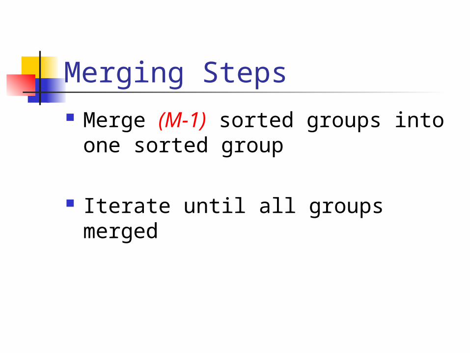
Merging Steps Merge (M-1) sorted groups into one

sorted group

Iterate until all groups merged

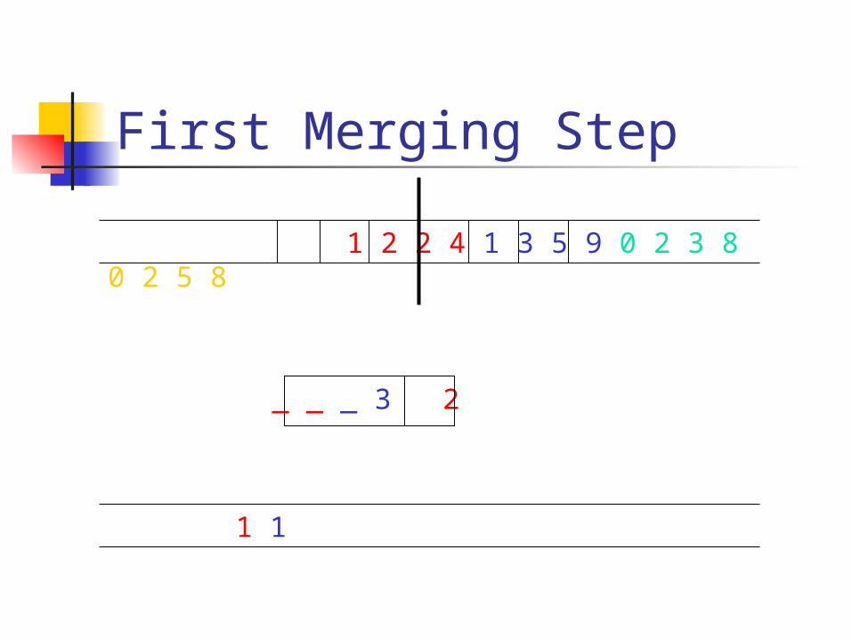
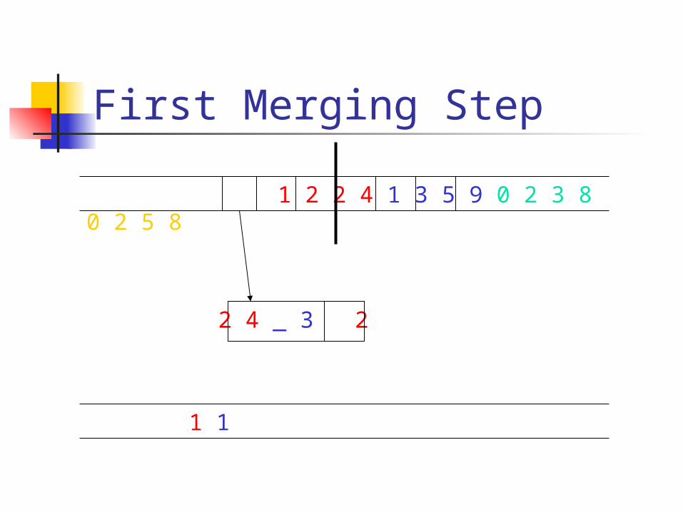
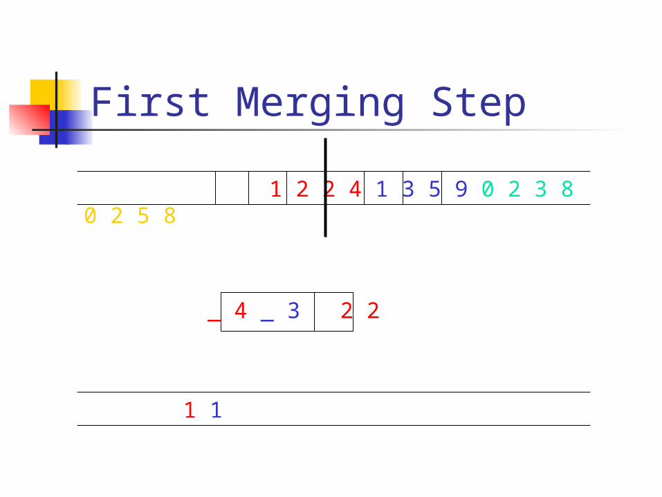
First Merging Step

1 2 1 3

1 2 2 4 1 3 5 9 0 2 3 8 0 2 5 8

N = 8M-1 = 2

First Merging Step

_ 2 _ 3 1 1

1 2 2 4 1 3 5 9 0 2 3 8 0 2 5 8

First Merging Step

_ 2 _ 3

1 2 2 4 1 3 5 9 0 2 3 8 0 2 5 8

1 1

First Merging Step

_ _ _ 3 2

1 2 2 4 1 3 5 9 0 2 3 8 0 2 5 8

1 1

First Merging Step

2 4 _ 3 2

1 2 2 4 1 3 5 9 0 2 3 8 0 2 5 8

1 1

First Merging Step

_ 4 _ 3 2 2

1 2 2 4 1 3 5 9 0 2 3 8 0 2 5 8

1 1

First Merging Step

_ 4 _ 3

1 2 2 4 1 3 5 9 0 2 3 8 0 2 5 8

1 1 2 2

End of First Merge

1 2 2 4 1 3 5 9 0 2 3 8 0 2 5 8

1 1 2 2 3 4 5 9 0 0 2 2 3 5 8 8

Start of Second Merge

1 1 2 2 3 4 5 9 0 0 2 2 3 5 8 8

1 1 0 0

End of Second Merge

1 1 2 2 3 4 5 9 0 0 2 2 3 5 8 8

0 0 1 1 2 2 2 2 3 3 4 5 5 8 8 9

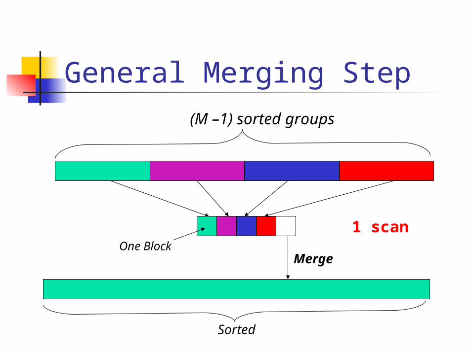
General Merging Step

Sorted

1 scan

(M –1) sorted groups

One BlockMerge

Overall Algorithm Repeat merging till all data sorted

N/(M-1) sorted groups to start with Merge (M-1) sorted groups into one

sorted group O(log N / log M) iterations Each iteration involves one scan of the data

O(log N/ log M) scans: Alternatively, N log N/ log M seeks

Lower Bounds for Sorting

Aggrawal and Vitter, 1988

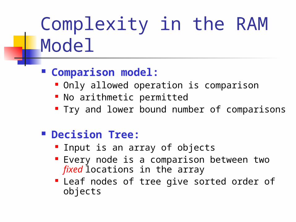
Complexity in the RAM Model Comparison model:

Only allowed operation is comparison No arithmetic permitted Try and lower bound number of comparisons

Decision Tree: Input is an array of objects Every node is a comparison between two

fixed locations in the array Leaf nodes of tree give sorted order of objects

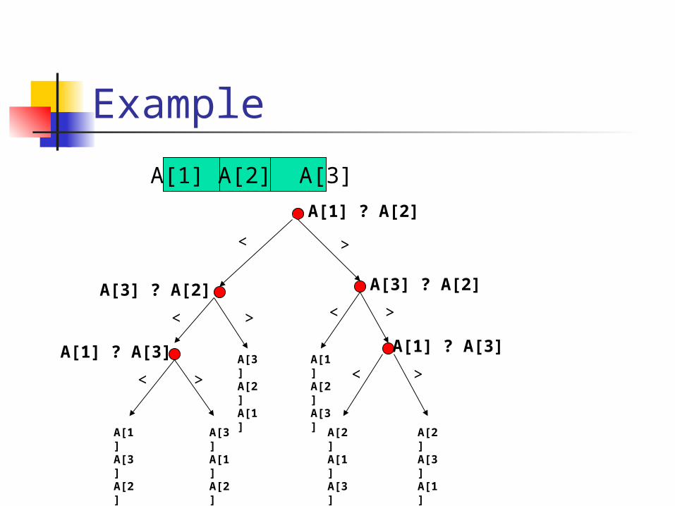
Example

A[1] A[2] A[3]

A[1] ? A[2]

< >

A[3] ? A[2]A[3] ? A[2]>

A[1] A[2] A[3]

<>

A[3] A[2] A[1]

<

< > ><A[1] ? A[3] A[1] ? A[3]

A[1] A[3] A[2]

A[3] A[1] A[2]

A[2] A[1] A[3]

A[2] A[3] A[1]

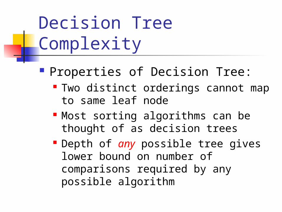
Decision Tree Complexity Properties of Decision Tree:

Two distinct orderings cannot map to same leaf node

Most sorting algorithms can be thought of as decision trees

Depth of any possible tree gives lower bound on number of comparisons required by any possible algorithm

Complexity of Sorting Given n objects in array:

Number of possible orderings = n! Any decision tree has branching

factor 2 Implies depth log (n!) = (n log n)

What about disk seeks needed?

I/O Complexity of Sorting Input has NB elements

Main memory size can store MB elements We know the ordering of all elements in

main memory What does a new seek do:

Read in B array elements New information obtained:

Ordering of B elements Ordering of (M-1)B elements already in memory

with the B new elements

Example Main memory has A < B < C

We read in D,E Possibilities:

D < E: D E A B C D A E B C A D B E C …

D > E: E D A B C E A D B C A E B D C …

20 possibilities in all

Fan Out of a Seek Number of possible outcomes of the

comparisons:

This is the branching factor for a seek

We need to distinguish between possible outcomes

( )!! exp( log( ))

( )!

MB MBB B MB

B MB B

( )!NB

Merge Sort Is Optimal

log(( )!) log( )Depth of Tree =

log( )( )!log

( )!

NB NBN

MBMBMB B

Merge Sort is almost optimal

Upper Bound for Merge Sort = O(N log N/ log M)

Improved Lower Bound Relative ordering of B elements in

block unknown iff block never seen before Only N such seeks In this case, possible orders =

Else, possible orders =

!MB

BB

MB

B

Better Analysis Suppose T seeks suffice For some N seeks:

Branching factor =

For the rest of the seeks: Branching factor =

!MB

BB

MB

B

Final Analysis

( !) ( )!

log log

log log

T

N MBB NB

B

NB N N NT

B M M

Merge Sort is optimal!

Some Notation Sort(X):

Number of seeks to sort X objects

Scan(X): Number of seeks to scan X objects =

log /

log

X BX

B M

X

B

Graph Connectivity

Munagala and Ranade, 1999

Problem Statement V vertices, E edges

Adjacency list: For every vertex, list the adjacent vertices O(E) elements, or O(E/B) blocks

Goal: Label each vertex with its connected component

Breadth First Search Properties of BFS:

Vertices can be grouped into levels

Edges from a particular level go to either:

Previous level Current level Next level

Notation Front(t) = Vertices at depth t

Nbr(t) = Neighbors of Front(t)

Example BFS Tree

Front(1)

Front(2)

Front(3)

Front(4)

Nbr(3)

Algorithm Scan edges adjacent to Front(t) to compute

Nbr(t)

Sort vertices in Nbr(t)

Eliminate: Duplicate vertices Front(t) and Front(t-1)

Yields Front(t+1)

Complexity I Scanning Front(t):

For each vertex in Front(t): Scan its edge list Vertices in Front(t) are not contiguous on

disk Round-off error of one block per vertex

O(Scan(E) + V) over all time t

Yields Nbr(t)

Complexity II Sorting Nbr(t):

Total size of Nbr(t) = O(E) over all times t Implies sorting takes O(sort(E)) I/Os

Total I/O: O(sort(E)+V)

Round-off error dominates if graph is sparse

PRAM Simulation

Chiang, Goodrich, Grove, Tamassia, Vengroff and Vitter

1995

PRAM Model

Memory

Parallel Processors

Model At each step, each processor:

Reads O(1) memory locations Performs computation Writes results to O(1) memory locations

Performed in parallel by all processors Synchronously! Idealized model

Terms for Parallel Algorithms Work:

Total number of operations performed

Depth: Longest dependency chain Need to be sequential on any parallel

machine

Parallelism: Work/Depth

PRAM Simulation Theorem: Any parallel algorithm with:

O(D) input data Performing O(W) work With depth one

can be simulated in external memory using O(sort(D+W)) I/Os

Proof Simulate all processors at once:

We write on disk the addresses of operands required by each processor

O(W) addresses in all

We sort input data based on addresses O(sort(D+W)) I/Os Data for first processor appears first, and so

on

More Proof Proof continued:

Simulate the work done by each processor in turn and write results to disk along

O(scan(W)) I/Os

Merge new data with input if required O(sort(D+W)) I/Os

Example: Find-min Given N numbers A[1…N] in array

Find the smallest number

Parallel Algorithm: Pair up the elements For each pair compute the smaller

number Recursively solve the N/2 size problem

Quality of Algorithm Work = N + N/2 + … = O(N)

Depth at each recursion level = 1 Total depth = O(log N)

Parallelism = O(N/log N)

External Memory Find Min First step: W = N, D = N, Depth = 1

I/Os = sort(N)

Second step: W = N/2, D = N/2, Depth = 1 I/Os = sort(N/2)

… Total I/Os = sort(N) + sort(N/2) + …

I/Os = O(sort(N))

Graph Connectivity Due to Chin, Lam and Chen, CACM 1982

Assume vertices given ids 1,2,…,V

Step 1: Construct two trees: T1: Make each vertex point to some

neighbor with smaller id T2: Make each vertex point to some

neighbor with larger id

Example

1

2

3

4

56

7

8

1

2

3

4

56

7

8

1

2

3

4

56

7

8

Graph T1 T2

Lemma One of T1 and T2 has at least V/2

edges Assuming each vertex has at least

one neighbor Proof is homework! Choose tree with more edges

Implementation Finding a larger/smaller id vertex:

Find Min or Find Max for each vertex O(E) work and O(log V) depth O(sort(E)) I/Os in external memory In fact, O(scan(E)) I/Os suffice!

Step 2: Pointer Doubling Let Parent[v] = Vertex pointed to by v

in tree If v has no parent, set Parent[v] = v

Repeat O(log V) times: Parent[v] = Parent[Parent[v]]

Each vertex points to root of tree to which it belongs

Implementation Work = O(V) per unit depth

Depth = O(log V)

I/Os = O(log V sort(V))

Total I/Os so far: O(scan(E) + log V sort(V))

Collapsing the Graph

2

56

7

1

9

1112

8

3

15

1314

10

4

1 3 4

Procedure Create new graph:

For every edge (u,v) Create edge (Parent[u], Parent[v]) O(E) work and O(1) depth O(scan(E)) I/Os trivially

Vertices: v such that Parent[v] = v Number of vertices at most ¾ V

Duplicate Elimination Sort new edge list and eliminate

duplicates O(E) work and O(log E) depth Parallel algorithm complicated O(sort(E)) I/Os trivially using Merge Sort

Total I/O so far: O(sort(E) + log V sort(V))

Iterate Problem size:

¾ V vertices At most E edges Iterate until number of vertices at most MB

For instance with V’ vertices and E’ edges: I/O complexity:

O(sort(E’) + log V’ sort(V’))

Total I/O Complexity

log ( )

3 3 log( ) ( ) log ...

4 4

log ( ) log( ) ( )

log( ) ( )

Vsort E

MB

V VV sort V sort

Vsort E V sort V

MB

V sort E

Comparison BFS Complexity:

O(sort(E) + V) Better for dense graphs (E > BV)

Parallel Algorithm Complexity: O(log V sort(E)) Better for sparse graphs

Best Algorithm Due to Munagala and Ranade, 1999

Upper bound:

Lower bound: (sort(E))

log log 1 ( )VB

O sort EE