External Debt and Economic Growth in Iran and Malaysia: A ...

Iranian Economic Review 2021, 25(2): 323-335

DOI: 10.22059/ier.2020.74562

RESEARCH PAPER

External Debt and Economic Growth in Iran and Malaysia:

A Smooth Transition Regression Model

Jalal Montazeri Shoorekchalia,*

, Ebrahim Eltejaeib

a, b. Department of Economics, Institute for Humanities and Cultural Studies, Tehran, Iran

Received: 25 May 2019, Revised: 21 September 2019, Accepted: 14 October 2019

© University of Tehran

Abstract

Since the debt crisis in the 1980s, the effect of external debt on economic growth has been a controversial

issue for economists. This paper aims to investigate the effects of external debt on economic growth in Iran

and Malaysia. Findings of a Smooth Transition Regression (STR) model support a nonlinear

relationship between the external debt size (the ratio of external debt stocks to GDP) and economic

growth in Iran and Malaysia over the period 1973–2017. Moreover, results of the STR models

estimation show that external debt affects Iranian economic growth in a two-regime structure with a

threshold of 2.96%, so that, the effect is negative in both regimes, but in the second regime as debt

increases, the negative effect becomes larger. Also, findings indicate that external debt size harms

Malaysian economic growth in a three-regime structure with two thresholds of 24.41% and 55.76%.

Finally, the mentioned negative effect is considerably less severe in Malaysia than in Iran.

Keywords: External Debt, Economic Growth, STR Model, Iran, Malaysia.

JEL Classification: C22, H63, O40.

Introduction

The experience of developing countries in the 1950s and 1960s indicates that most of them

relied largely on domestic resources rather than external resources to finance public

investment projects. In contrast, since 1970s, an increasing number of countries have adopted

debt-based growth approach (Ajayiand Oke, 2012: 297). In fact, foreign financial resources

helped those economies to develop, so that it created the economic miracle of Brazil and some

emerging Asian economies (Changyong et al., 2012: 158). In the 1980s, some countries,

particularly in Latin America, like Brazil, Argentina, and Mexico, faced difficulties to repay

their debts. Since the mid-1990s, the problem of high external debt of developing countries

has been considered by policymakers and has been recognized as a big obstacle for poor

countries in economic growth and development process.

Despite many difficulties, financing deficits by borrowing from foreign and international

resources has remained as a broadly used way. Some countries may need to borrow in early

stages of growth to achieve capital accumulation and ease economic growth. However, raising

the level of debt will lead to various risks. Economists have proposed various opinions and

theories in this view. Based on liquidity constraints hypothesis, in heavy indebted countries

repayment of debts requires lots of credit, which causes shortage of resources for investment

(Hofman and Reisen, 1991: 282). In standard overlapping generation's models, increasing

debts, due to reduction of saving and capital accumulation has negative effect on long-run

* Corresponding author email: [email protected]

https://dx.doi.org/10.22059/ier.2020.74562

324 Shoorekchali and Eltejaei

economic growth (Eberhardt and Presbitero, 2015: 3). Based on debt overhang theory, a high

level of general debts, due to substitution effect, has negative effects on domestic saving and

investment, so reduces economic growth (Krugman, 1988). This argument is represented in

the “debt Laffer curve”, which posits that larger debt tend to be associated with lower

economic growth, since it reduces total factor productivity (TFP) and lowers probabilities of

debt repayments (Karadam, 2018: 2). Therefore, debt-growth relationship may be nonlinear,

implying that debt is growth enhancing at lower debt/GDP ratio levels and growth reducing at

higher debt/GDP ratio levels (Eboreime and Sunday, 2017: 7).

Based on this theoretical literature, empirical investigation of the effects of external debt

on economic growth is important in each economy. Obviously, this importance is doubled in

developing countries, such as Iran, because of their low ratio of capital formation. In fact, the

main question is that, based on the “debt Laffer curve” theoretical framework, weather a

suggestion for developing countries can be made to hire external borrowed reserves below an

allowed ceiling to finance their productive investment projects, so these borrowed reserves

have no negative effects on their economic growth.

Also, this paper tries to use a comparative approach to compare the effects of external debt

on economic growth in Iran and Malaysia. However, it is supposed that Malaysian

experiments in using external debts are transferable to other developing countries like Iran.

There are some other reasons for selecting Malaysia as a comparative case:

Over the recent four decades, Malaysian economy has transited from a producer and

exporter of primary goods to an exporter of industrial goods. Currently, its industrial

sector share in GDP is four times larger than its agricultural sector share. So, Malaysian

economy may be a good model for the Iranian single product and oil based economy.

Comparing Iran and Malaysia based on external debt size and economic growth, shows

that both these variables were obviously greater than those of Iran during 1973-2017

period (figures 1 and 2). Malaysia and Iran respectively have experimented an average

of 46.84 and 6.61 percent for external debt/GDP ratio and an average of 6.21 and 2.09

percent for economic growth. Therefore, two questions are remarkable: first; how

external debt has affected economic growth in both economies? Second; does relying on

external debt in Malaysian economy, as a relatively successful developing country in

economic growth, have applied lessons for Iranian economy?

Figure 1. External Debt Stocks (% of GDP)

Source: World Development Indicators, 2019.

y = 0.0469x + 5.5332

y = 0.7214x + 30.253

0

10

20

30

40

50

60

70

80

90

1,9

73

1,9

75

1,9

77

1,9

79

1,9

81

1,9

83

1,9

85

1,9

87

1,9

89

1,9

91

1,9

93

1,9

95

1,9

97

1,9

99

2,0

01

2,0

03

2,0

05

2,0

07

2,0

09

2,0

11

2,0

13

2,0

15

2,0

17

Iran Malaysia Linear ( Iran) Linear (Malaysia)

19

73

19

75

19

77

19

79

19

81

19

83

19

85

19

87

19

89

19

91

19

93

19

95

19

97

19

99

20

01

20

03

20

05

20

07

20

09

20

11

20

13

20

15

Iranian Economic Review 2021, 25(2): 323-335 325

Figure 2. GDP Growth (annual %) Based on Constant 2000 U.S. $

Source: World Development Indicators (WDI), 2019.

In brief, this paper aims to investigate nonlinear effects of external debt size that is external

debt over GDP ratio on economic growth and compare this effect in Iran and Malaysia. Foe

this, a Smooth Transition Regression (STR) model on the data of 1973–2017 period is hired.

This paper is continued as follows. The next section presents a brief literature review on the

relationship between external debt and economic growth. In Section 3, the models are presented

followed by Estimation of Smooth Transition Regression (STR) models in section4. Finally,

concluding remarks are given in Section 5.

Literature Review

Generally, budget deficit can be financed by domestic or international resources. In absence of a

strong private sector and an efficient banking system, domestic resources are not responsible

and many poor countries borrow from international lenders and other external resources.

External debt affects economic growth through two channels. First, through the debt overhang

effect, that states when debt level increases, investors expect rising taxes in the future; this,

affect total investment, especially private investment, negatively. Second, through debt

crowding out effect, that says when export revenues go to repayment debt stocks, no

resources remain for investment, so economic growth reduces (Ejigayehu, 2013:3).

Presbitero (2012) states that industrial countries use borrowed funds in sectors which are

more productive better than developing countries. Therefore, they control better the negative

consequences of debts, such as crowding out effect, disincentive environment to investment,

political uncertainty, and capital outflow due to anxiety about national currency devaluation.

Thus, external debt, due to weak management, has a negative effect on the economic growth

of poor countries (Kharusi and Ada, 2018:1144).

It is said, generally, that a low or reasonable level of debts probably increase economic

growth, but high-level debts decrease it. This is known as nonlinearity or asymmetry effecting

of external debt on economic growth. Countries that borrow in early stages of growth,

actually want to benefit from investment opportunities with higher rate of return. In other

words, these countries can improve economic growth through productive investments that are

financed by borrowed funds. Nevertheless, raising the level of debt will lead to various risks.

When the debt stocks increase, the repayment ability will be more sensitive to income level

-40

-30

-20

-10

0

10

20

30

1,9

73

1,9

75

1,9

77

1,9

79

1,9

81

1,9

83

1,9

85

1,9

87

1,9

89

1,9

91

1,9

93

1,9

95

1,9

97

1,9

99

2,0

01

2,0

03

2,0

05

2,0

07

2,0

09

2,0

11

2,0

13

2,0

15

2,0

17

Iran Malaysia

19

73

19

75

19

77

19

79

19

81

19

83

19

85

19

87

19

89

19

91

19

93

19

95

19

97

19

99

20

01

20

03

20

05

20

07

20

09

20

11

20

13

20

15

20

17


and interest rates, meanwhile, a negative shock, will severely have negative effect on the level

of economic activity (Karadam, 2018: 1–2). Therefore, high-level debt stocks will lead to

increase fluctuations in real sector, fragility of financial sector, and decline average long-run

economic growth. Theoretically, this argument is offered under the “theory of optimal level

for government debt”. Based on this theory, there is an inverted U relationship between

government debt/GDP ratio and economic growth (Figure 1), in which up to a certain

threshold, increasing the ratio, because of increasing savings (since the government replaces

borrowing for taxes to offset the deficit) has a positive effect on economic growth. Beyond

that, increasing debt/GDP ratio, due to crowding out effect, causes a decline in long-run

economic growth (Eboreimand Sunday, 2017:8).

Figure 1. Nonlinear Relationship between Debt/GDP Ratio and Economic Growth

Source: Eboreimand Sunday, 2017: 8.

In summary, it can be said that asymmetric or nonlinear effect of government debt on

economic growth, is more consistent with the economic realities because of three main points:

First, debt is an unavoidable part of government finance. Second, depending on economic

conditions and structures, debt can have different economic consequences. In other words,

debt is a double-edged sword, which if there is economic stability, it will act as an economic

stimulus, but in the case of wasteful growing debt stocks, it raises uncertainty and narrows

private sector access to financial resources and savings, and acts as a barrier to economic

growth. Third, according to Jiménez (2011), the efficiency of government debt depends on the

economy condition and government financial situation.

Empirically, the effect of external debt on economic growth has been discussed in various

studies. Kharusi and Ada (2018) using an Autoregressive Distributed Lag (ARDL)

Cointegration model showed that external debt has negative effect on economic growth of

Jordan during 1990-2015. Before, similar findings were reported by Akram (2011), and Rais

and Anwar (2012) in Pakistan by the time series of 1972-2009 and 1972-2010; Umaru et al.

(2013) and Mbah et al. (2016) in Nigeria in 1970-2010 and 1970-2013; Calderón and Fuentes

(2013) in Latin American countries during 1970-2010 and Tchereni et al. (2013) in Malawi

during 1975-2003.

On the contrary, some studies have showed positive effect of external debt on economic

growth. Korkmaz (2015) using seasonal data on 2003:1-2014:3 in Turkey showed a one-way

causality and positive effect of external debt on economic growth. Also, Kadiu (2015)

reported this positive effect in Albany during 1991-2012, Ebi et al. (2013) and Utomi (2014)

in Nigeria during 1970-2011 and 1980-2012 and in Zaman and Arslan (2014) in Pakistan

during 1972-2010.

In addition, nonlinear relationship between external debt and economic growth has been

studied empirically in some papers. Doğan and Bilgili (2014) by Turkish time series data

during 1974-2009 using a Markov-switching model show that economic growth and


borrowing variables have negative relationship but do not follow a linear path. Dao and Oanh

(2017) using Johansen-Juselius technique on Vietnamese seasonal data during 2000-2012

have confirmed inverted U-shaped relationship between external debt and economic growth

and showed the threshold point at 28%. Haron and Maingi (2018) examined this nonlinear

relationship in Kenya during 1970-2017, using a Generalized Method of Moments (GMM)

model and estimated the mentioned threshold at about 61%.

The Model

Based on theoretical framework of debt Laffer curve, the impacts of external debt size on

economic growth are not the same in various observations and follow a nonlinear pattern.

Therefore, very likely the dynamic relationship between variables is not constant and depends

on the concurrent state of the economy. Generally, modeling this case involves using

approaches that consider threshold limits such as “Threshold Regression (TR)”, “Smooth

Transitional Regression (STR)”, “Artificial Neural Networks (ANN)” and “Markov

Switching Model”. In this paper we use a STR model to investigate the nonlinear effects of

external debt on economic growth based on the debt Laffer curve. Compared with other

approaches, the STR model has some advantages as:

The STR model considers regime switching or structural changes directly within the

model and there is no need to enter dummy variables or to check structural changes by

additional diagnostic tests.

The STR model shows regime switching speed in addition to the number and the time

of regime switching. The STR model is a specific case of TR models.

Although the ANN approach has a good fit on data, but it involves an important

problem that has no clear economic interpretation. When the number of connected units

or nodes, that are called artificial neurons, is very big, the model will be over-fitted. But

in the STR model the coefficients have clear interpretation.

In Markov Switching model the regime switching is exogenous, but this is endogenous

in STR model (Enders 2004, Van Dijk et.al 2000).

According to Teräsvirta (1994), for considering the nonlinear effects of external debt size

on economic growth, we specify a nonlinear structure based on the smooth transition

regression (STR) model as follows:

0 1 * ( , , )t t t tEG x Z g EDS c (1)

Where, EG is economic growth, EDS is the external debt size (that is the ratio of external debt

stocks over GDP), and Z is the vector of explanatory variables consist of current and lagged

values of EDS and lagged values of economic growth. 0 and 1 are the vectors of linear and

nonlinear part coefficients. t is an independent and identically distributed (i.i.d.) process

with zero mean and finite variance. So, ),0( 2 iidt . Assuming a two-regime transition

function in which regime change occurs once, the logistic function is as follows:

1

1( , , ) 1 exp ( ) 0

t

k

t k tk

d

g EDS c EDS c with

(2)

Where, g is a transition function bounded by zero and one (where g becomes Heaviside).

Additionally, ( , , ) 0.5g EDS c ; therefore, we can say that the location parameter c


represents the point of transition between the two extreme regimes with lim 0ts g and

lim 1ts g . k is a parameter to show the number of regime changes. The slope parameter

indicates how rapidly the transition of g from zero to one takes place. When , if cst ,

then 1g , and if cst , then 0g . Therefore, the Equation (1) will be a threshold

regression (TR) model. When 0 , the Equation (2) becomes a linear regression model

(Van Dijk, 1999; Teräsvirta, 2004).

In the case of a three-regime model in which two regime-changes occur, Jansen and

Teräsvirta (1996) propose the logistic function as the following form:

1 2

1( , , )

1 exp ( )( )t

t t

g EDS cEDS c EDS c

0,21 cc (3)

In this case, when 0 , the model will be linear and when , for 1tEDS c and

2tEDS c , we will have ( , , ) 1tg EDS c , and for 1 2tc EDS c , we will have

( , , ) 0tg EDS c . Meanwhile, G is symmetric about the point 2

21 cc and lim 1

ts g .

In general, STR modeling includes three steps:

1) Specification starts with setting up a linear model that forms a starting point for the

analysis. It can be modelled by using the VAR framework. The second part of

specification involves testing for nonlinearity, choosing transition variable and deciding

whether LSTR1or LSTR2 should be used.

2) Estimation involves finding appropriate starting values for the nonlinear estimation and

estimating the model.

3) Evaluation of the model usually includes various tests for problems such as error

autocorrelation, parameters stability, remaining nonlinearity, ARCH and non-normality.

Empirical Results

As said before, the first step in the STR modeling is to specify an adequate linear model and

determine the number of lags for relevant variables, in order to capture the dynamic process.

Since, we want to investigate nonlinear effect of external debt size (EDS) on economic

growth (EG) in Iran and Malaysia; we only include the EDS and its lagged values as

explanatory variables. According to the number of observations (that are less than 100), the

optimal lags are determined based on Schwarz Bayesian Criterion (SBC). Next, it is necessary

to test the null hypothesis of linearity against nonlinearity as the alternative hypothesis. If the

transition variable is unknown, then the test haste is repeated for every potential transition

variable. If the null cannot be rejected in any case, then we conclude that the linear model is

appropriate and there is no need to proceed with STR models. But, if the null hypothesis is

rejected for any transition variable, then we must use a STR model to capture the full behavior

of the time series. If the null can be rejected more than once in favor of the STR models, then

the model with the strongest rejection (lowest p-value) is selected to be estimated. In brief, we

test the null of linearity against the alternative hypothesis of STR model and decide for the

appropriate transition variable and the number of regimes based on F, F2, F3, and F4 statistics.

The results of this step, reported in Table 1, indicate that the null hypothesis of linear

relationship between the variables can be rejected at 5% level of significance only for 2tEDS

in Iran and for tEDS in Malaysia, and these variables are selected as the transition variables.


Also, based on the test statistics F2, F3, and F4 reported in Table 1, for the transition variable

2tEDS , the logistic model with one threshold (LSTR1) and for the transition variable tEDS ,

the logistic model with two threshold (LSTR2) are selected as the appropriate models.

Table 1. The Results of the Linearity Tests Against the STR Model

Country Transmission

variable

P-value of the

F-statistic

P-value of the

F2-statistic

P-value of the

F3-statistic

P-value of the

F4-statistic

Proposed

model

Iran

EDS(t) 0.79 0.85 0.21 0.84 Linear

EDS(t-1) 0.37 0.04 0.11 0.78 Linear

EDS(t-2) 0.04 0.004 0.62 0.08 LSTR1

EDS(t-3) 0.26 0.03 0.77 0.32 Linear

EDS(t-4) 0.08 0.10 0.61 0.08 Linear

Malaysia EDS(t) 0.001 0.37 0.002 0.01 LSTR2

EDS(t-1) 0.11 0.63 0.18 0.06 Linear

Source: Research finding.

Now, having determined the transition variables we can estimate the models using the

Newton-Raphson algorithm and maximum likelihood method. Results for each country, Iran

and Malaysia are reported in Tables 2 and 3.

Table 2. Results of Model Estimation - Iran

Coefficient T-statistic P-value

Linear Part

CONST 0.23 2.89 0.01

EG(t-2) -1.95 -3.45 0.00

EG(t-3) -2.57 -3.52 0.00

EG(t-4) -1.65 -3.84 0.00

EDS(t) -1.23 -3.87 0.00

EDS(t-1) -0.86 -2.57 0.02

EDS(t-3) 2.26 3.18 0.00

EDS(t-4) -1.35 -2.63 0.01

Nonlinear Part

CONST -0.16 -1.94 0.06

EG(t-2) 1.34 2.33 0.03

EG(t-3) 2.56 3.46 0.00

EG(t-4) 1.58 3.52 0.00

EDS(t) 1.26 3.95 0.00

EDS(t-1) -0.83 -2.46 0.02

EDS(t-3) -2.26 -3.18 0.00

EDS(t-4) 1.34 2.60 0.02

Adjusted R2: 86.76 AIC: -6.01

SC: -5.26 HQ: -5.74

Note: coefficients, which are not statistically significant, excluded in the final model.



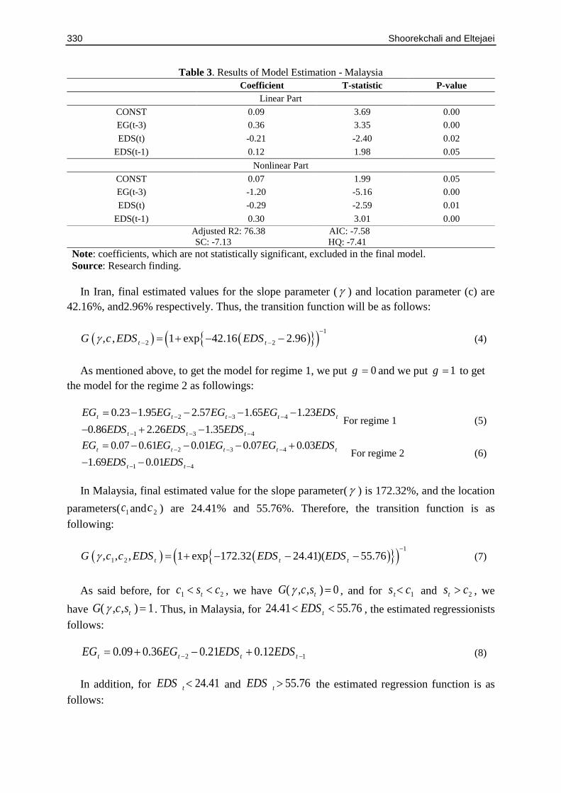
Table 3. Results of Model Estimation - Malaysia

Coefficient T-statistic P-value

Linear Part

CONST 0.09 3.69 0.00

EG(t-3) 0.36 3.35 0.00

EDS(t) -0.21 -2.40 0.02

EDS(t-1) 0.12 1.98 0.05

Nonlinear Part

CONST 0.07 1.99 0.05

EG(t-3) -1.20 -5.16 0.00

EDS(t) -0.29 -2.59 0.01

EDS(t-1) 0.30 3.01 0.00

Adjusted R2: 76.38 AIC: -7.58

SC: -7.13 HQ: -7.41

Note: coefficients, which are not statistically significant, excluded in the final model.


In Iran, final estimated values for the slope parameter ( ) and location parameter (c) are

42.16%, and2.96% respectively. Thus, the transition function will be as follows:

1

2 2, , 1 exp 42.16 2.96

t tG c EDS EDS (4)

As mentioned above, to get the model for regime 1, we put 0g and we put 1g to get

the model for the regime 2 as followings:

2 3 4

1 3 4

0.23 1.95 2.57 1.65 1.23

0.86 2.26 1.35

t t t t t

t t t

EG EG EG EG EDS

EDS EDS EDS

For regime 1 (5)

2 3 4

1 4

0.07 0.61 0.01 0.07 0.03

1.69 0.01

t t t t t

t t

EG EG EG EG EDS

EDS EDS

For regime 2 (6)

In Malaysia, final estimated value for the slope parameter( ) is 172.32%, and the location

parameters( 1c and 2c ) are 24.41% and 55.76%. Therefore, the transition function is as

following:

1

1 2, , , 1 exp 172.32 24.41)( 55.76

t t tG c c EDS EDS EDS (7)

As said before, for 21 csc t , we have 0),,( tscG , and for 1cs t and 2cst , we

have 1),,( tscG . Thus, in Malaysia, for 24.41 55.76tEDS , the estimated regressionists

follows:

2 10.09 0.36 0.21 0.12t t t tEG EG EDS EDS (8)

In addition, for 24.41tEDS and 55.76tEDS the estimated regression function is as

follows:


3 10.16 0.84 0.50 0.42t t t tEG EG EDS EDS (9)

In order to show corresponding years with different regimes, the trend of external debt size

and its threshold are presented in Figure 3 for the Iranian economy. As is seen, the first

regime covers the years of 1973–1979 and 2011–2017, in which the external-debt/GDP ratio

was less than 2.96%. The second regime covers the years of 1980–2010, in which the debt

size was larger than 2.96%. In addition, based on nonlinear estimated regression for Iran -

equations (5) and (6) -during the first regime, the sum of coefficients for current and lagged

EDS is -1.18. This summation for the second regime is-1.67. Therefore, it can be said that

external debt had always a negative effect on economic growth in Iranian economy, although

in the second regime, as the debt size increases, this negative effect becomes larger.

Figure 3. External Debt Size and Its Threshold in the Iran


Figure 4 shows the corresponding years with different regimes based on the nonlinear

estimated regression for Malaysian economy. The figure shows that, the first regime includes

the year’s of1973–1975, in which the debt/GDP ratio was less than 24.41%. The second

regime covers the periods 1976–1982, 1988–1997, 2000–2009, and 2011–2012, in which the

debt/GDP ratio was larger than 24.41% and smaller than 55.76%, and the third regime

includes the periods 1983–1987, 1998–1999, 2010, and 2012–2017, in which the debt/GDP

ratio was larger than 55.76%.

Based on equations (8) and (9), during the first and third regimes, the sum of coefficients

for current and lagged EDSs is -0.08. This summation for the second regime is -0.09.

Therefore, it can be said that, like Iranian economy, external debt in Malaysia had always a

negative effect on economic growth, although this negative effect is considerably less severe

in Malaysia than Iran.

0

5

10

15

20

25

30

35

40

19

73

19

75

19

77

19

79

19

81

19

83

19

85

19

87

19

89

19

91

19

93

19

95

19

97

19

99

20

01

20

03

20

05

20

07

20

09

20

11

20

13

20

15

20

17

External Debt Size Threshold

19

73

19

75

19

77

19

79

19

81

19

83

19

85

19

87

19

89

19

91

19

93

19

95

19

97

19

99

20

01

20

03

20

05

20

07

20

09

20

11

20

13

20

15

20

17


Figure 4. External Debt Size and Its Threshold in the Malaysia


In the next step, the estimated STR model must be evaluated using misspecification and

diagnostic tests such as no error-autocorrelation, no additive nonlinearity, parameters stability,

ARCH and Jarque-Bera test. Results of diagnostic tests are reported in Table 4. Based on the

inference results, the quality of the estimated nonlinear models is acceptable.

Table 4. Diagnostic Tests Results

P-Value of F-statistic Test

0.17<p-value F(lag 1 to 8)<0.82 Test of no error term autocorrelation

Iran

p-value F=0.52 Test of no remaining nonlinearity

p-value F(H1)=0.01 Parameter constancy test

p-value F=0.82 and p-value (Chi^2)=0.88 ARCH-LM test with 8 lags

p-value (Chi^2)=0.96 JARQUE-BERA test

0.09<p-value F(lag 1 to 8)<0.87 Test of no error autocorrelation

Malaysia

p-value F=0.44 Test of no remaining nonlinearity

p-value F(H1)=0.04 Parameter constancy test

p-value F=0.84 and p-value (Chi^2)=0.78 ARCH-LM test with 8 lags

p-value (Chi^2)=0.88 JARQUE-BERA test


Conclusion

The debt-growth relationship has received renewed interest among academics and policy

makers alike in the aftermath of the recent decade's financial crisis. This paper empirically

compares the nonlinear effect of external debt size on the economic growth between Iran and

Malaysia using a Smooth Transition Regression (STR) model.

Our results show: First, there is a nonlinear behavior between the external debt size (the

ratio of external debt stocks to GDP) and economic growth in Iran and Malaysia over the

period 1973–2017.Second, external debt size affects Iran's economic growth in a two-regime

structure with a threshold in 2.96%, So that, this effect is negative in both regimes, but in the

second regime, with increasing debt size, this negative effect becomes larger. Third, external

debt size has a negative effect on Malaysian economic growth in a three-regime structure with

0

10

20

30

40

50

60

70

80

90

External Debt Size First Threshold Second Threshold

19

73

19

75

19

77

19

79

19

81

19

83

19

85

19

87

19

89

19

91

19

93

19

95

19

97

19

99

20

01

20

03

20

05

20

07

20

09

20

11

20

13

20

15

20

17


two thresholds in 24.41% and 55.76%, although this negative effect is considerably less

severe in Malaysia than Iran.

As a summation based on findings of this research, there have been no evidences for

positive effects of external debt on economic growth in Iran and Malaysia. As Ajayi (1991)

stated this negative effect could be occurred through two channels:

a) Through the debt overhang effect: a situation when an accumulated debt, discourage and

overhang investment, mainly private investment; as private investors expect an increase in tax

by government to pay the accumulated debt

b) Through debt crowding out effect, that is a situation when export revenues are used to

pay the accumulated debt. This in turn may affects investment.

Also, this negative effect can be attributed to the development economists’ critique. They

believe that borrowing from abroad basically is not able to provide basis for real development

due to provoking corruption and expanding autonomous and costly bureaucracies. Malaysian

economy although has experienced a stable high level economic growth, external debt not

only had no positive role in this scenario but also with its negative role has decelerated it.

Hence, relying on external debt in Malaysia is not the experience that Iran should follow to

stimulate its economic growth.

Therefore, based on the findings of this paper, it is recommended that financing by external

borrowing, at least for the short-run, as long as there is no proper planning for this type of

funds, be excluded from the financing portfolio of the countries under study. This

recommendation is more important for Iran, since this negative effect of external debt is

considerably more severe than Malaysia.

References

[1] Ajayi, L. B., & Oke, M. O. (2012). Effect of External Debt on Economic Growth and

Development of Nigeria. International Journal of Business and Social Science, 3(12), 297-304.

[2] Ajayi, S. I. (1991). Macroeconomic Approach to External Debt the Case of Nigeria. AERC

Research Papers Series, 8, Retrieved from https://aercafrica.org/wp-

content/uploads/2018/07/RP8.PDF.

[3] Akram, N. (2011). Impact of Public Debt on the Economic Growth of Pakistan. The Pakistan

Development Review, 50(411), 599-615.

[4] Calderón, C., & Fuentes, J. R. (2013). Government Debt and Economic Growth. IDB Working

Paper Series, IDB-WP-424, Retrieved from

https://pdfs.semanticscholar.org/dfe4/1b937ebd2540b06bfd5cf8ebda2899c87a97.PDF.

[5] Changyong, X., Jun, S., & Chen, Y. (2012). Foreign Debt, Economic Growth and Economic

Crisis. Journal of Chinese Economic and Foreign Trade Studies, 5(2), 157-167.

[6] Dao, H. T. T., & Oanh, D. H. (2017). External Debt and Economic Growth in Vietnam: A

Nonlinear Relationship. China-USA Business Review, 16(1), 1-13.

[7] Doğan, I., & Bilgili, F. (2014). The Non-Linear Impact of High and Growing Government

External Debt on Economic Growth: A Markov Regime-switching Approach. Economic

Modelling, 39(C), 213-220.

[8] Eberhardt, M., & Presbitero, A. F. (2015). Public Debt and Growth: Heterogeneity and Non-

Linearity. Journal of International Economics, 97(1), 45-58.

[9] Ebi, B. O., Abu, O., & Clement, D. (2013). The Relative Potency of External & Domestic Debts

on Economic Performance in Nigeria. European Journal of Humanities and Social Sciences,

27(1), 1415-1429.


[10] Eboreime, M. I., & Sunday, B. (2017). Analysis of Public Debt-Threshold Effect on Output

Growth in Nigeria. EconWorld, Retrieved from

https://paris2017.econworld.org/papers/Eboreime_Analysis.PDF.

[11] Ejigayehu, D. A. (2013). The Effect of External Debt on Economic Growth: A Panel Data

Analysis on the Relationship between External Debt and Economic Growth. Retrieved from

http://www.diva-portal.org/smash/get/diva2:664110/FULLTEXT01.PDF.

[12] Enders, W. (2004). Applied Econometric Time Series. Technometrics, 46(2), 264-270.

[13] Hofman, B., & Reisen, H. (1991). Some Evidence on Debt-Related Determinants of Investment

and Consumption in Heavily Indebted Countries. Weltwirtschafliches Archiv, 127(2), 280-297.

[14] Haron, K. N., & Maingi, J. (2018). He Non-Linear Effect of High and Growing External Debt on

Kenya’s Economy. International Journal of Economics, Commerce and Management, 6(11), 41-57.

[15] Jansen, E. S., & Teräsvirta, T. (1996). Testing Parameter Constancy and Super Erogeneity in

Econometric Equations. Oxford Bulletin of Economics and Statistics, 58(4), 735–768.

[16] Kadiu, F. (2015). Public Debt & Economic Growth: Case of Albania. Global Advance Research

Journal of Management and Business Studies, 4(5), 186-189.

[17] Karadam, D. Y. (2018). An Investigation of Nonlinear Effects of Debt on Growth. The Journal of

Economic Asymmetries, Retrieved from

https://www.sciencedirect.com/science/article/pii/S1703494918300173

[18] Kharusi, S. A., & Ada, M. S. (2018). External Debt and Economic Growth: The Case of

Emerging Economy. Journal of Economic Integration, 33(1), 1141-1157.

[19] Krugman, P. (1988). Financing vs. Forgiving a Debt Overhang. Journal of Development

Economics, 29(3), 253-268.

[20] Korkmaz, S. U. N. A. (2015). The Relationship between External Debt and Economic Growth in

Turkey. Proceedings of the Second European Academic Research Conference on Global

Business, Economics, Finance and Banking (EAR15Swiss Conference), Retrieved from

ttps://pdfs.semanticscholar.org/5571/61aee7a378002a070a74d7a75876f3847d2b.PDF

[21] Mbah, S. A., Agu O. C., & Umunna G. (2016). Impact of External Debt on Economic Growth in

Nigeria: An ARDL Bound Testing Approach. Journal of Economics and Sustainable

Development, 7(10), 16-26.

[22] Presbitero, A. F. (2012). Total Public Debt and Growth in Developing Countries. The European

Journal of Development Research, 24(4), 606-626.

[23] Rais, S. I., & Anwar, T. (2012). Public Debt and Economic Growth in Pakistan: A Time Series

Analysis from 1972 to 2010. Academic Research International, 2(1), 535.

[24] Tchereni, B. H. M., Sekhampu, T. J., & Ndovi, R. F. (2013). The Impact of Foreign Debt on

Economic Growth in Malawi. African Development Review, 25(1), 85-90.

[25] Teräsvirta, T. (2004). Smooth Transition Regression Modelling. In H. Lutkepohl and M. Kratzig

(Eds.), Applied Time Series Econometrics. New York: Cambridge University Press.

[26] ---------- (1994). Specification, Estimation, and Evaluation of Smooth Transition Autoregressive

Models. Journal of the American Statistical Association, 89(425), 208-218.

[27] Umaru, A., Hamidu, A. A., & Musa, S. (2013). External Debt and Domestic Debt Impact on the

growth of the Nigerian Economy. International Journal of Educational Research, 1(2), 70-85.

[28] Utomi, W. (2014). The Impact of External Debt on Economic Growth in Nigeria (Doctoral

Dissertation, Covenant University, Nigeria). Retrieved from

http://eprints.covenantuniversity.edu.ng/2641/1/External%20debt%20and%20growth.PDF.

[29] Van Dijk, D. (1999). Smooth Transition Models: Extensions and Outlier Robust Inference.

(Doctoral Dissertation, Erasmus University Rotterdam, Netherlands), Retrieved from

https://repub.eur.nl/pub/1856/fewdis20020501113139.PDF.

http://www.tinbergen.nl/alumni-association/alumni.php?id=200

https://repub.eur.nl/pub/1856/fewdis20020501113139.pdf


[30] Van Dijk, D., Trasvirta, T., & Franses, P. H. (2000). Smooth Transition Autoregressive Models-a

Survey of Recent Developments. Econometric Reviews, 21(1), 1-47.

[31] Zaman, R., & Arslan, M. (2014). The Role of External Debt on Economic Growth: Evidence

from Pakistan Economy. Journal of Economics and Sustainable Development, 5(24), 140-148.

This article is an open-access article distributed under the terms and conditions

of the Creative Commons Attribution (CC-BY) license.

External Debt and Economic Growth in Iran and Malaysia: A ...

Documents

Transcript of External Debt and Economic Growth in Iran and Malaysia: A ...