Extensive Analysis of a Real-Time Dense Wired Sensor ...
29
This is a repository copy of Extensive Analysis of a Real-Time Dense Wired Sensor Network Based on Traffic Shaping. White Rose Research Online URL for this paper: https://eprints.whiterose.ac.uk/131890/ Version: Accepted Version Article: Loureiro, Joao, Rangarajan, Raghuraman, Nikolic, Borislav et al. (2 more authors) (2019) Extensive Analysis of a Real-Time Dense Wired Sensor Network Based on Traffic Shaping. ACM Transactions on Cyber-Physical Systems. 27. ISSN 2378-9638 https://doi.org/10.1145/3230872 [email protected] https://eprints.whiterose.ac.uk/ Reuse Items deposited in White Rose Research Online are protected by copyright, with all rights reserved unless indicated otherwise. They may be downloaded and/or printed for private study, or other acts as permitted by national copyright laws. The publisher or other rights holders may allow further reproduction and re-use of the full text version. This is indicated by the licence information on the White Rose Research Online record for the item. Takedown If you consider content in White Rose Research Online to be in breach of UK law, please notify us by emailing [email protected] including the URL of the record and the reason for the withdrawal request.
Transcript of Extensive Analysis of a Real-Time Dense Wired Sensor ...

This is a repository copy of Extensive Analysis of a Real-Time Dense Wired Sensor Network Based on Traffic Shaping.
White Rose Research Online URL for this paper:https://eprints.whiterose.ac.uk/131890/
Version: Accepted Version
Article:
Loureiro, Joao, Rangarajan, Raghuraman, Nikolic, Borislav et al. (2 more authors) (2019) Extensive Analysis of a Real-Time Dense Wired Sensor Network Based on Traffic Shaping. ACM Transactions on Cyber-Physical Systems. 27. ISSN 2378-9638
https://doi.org/10.1145/3230872
[email protected]://eprints.whiterose.ac.uk/
Reuse
Items deposited in White Rose Research Online are protected by copyright, with all rights reserved unless indicated otherwise. They may be downloaded and/or printed for private study, or other acts as permitted by national copyright laws. The publisher or other rights holders may allow further reproduction and re-use of the full text version. This is indicated by the licence information on the White Rose Research Online record for the item.
Takedown
If you consider content in White Rose Research Online to be in breach of UK law, please notify us by emailing [email protected] including the URL of the record and the reason for the withdrawal request.
1
Extensive Analysis of a Real-Time Dense Wired Sensor
Network Based on Traffic Shaping
JOÃO LOUREIRO, CISTER/INESC-TEC, ISEP, Polytechnic Institute of Porto, PortugalRAGHURAMAN RANGARAJAN, CISTER/INESC-TEC, ISEP, Polytechnic Institute of Porto, PortugalBORISLAV NIKOLIC, CISTER/INESC-TEC, ISEP, Polytechnic Institute of Porto, Portugal; Institute ofComputer and Network Engineering, Technische Universität Braunschweig, Germany
LEANDRO SOARES INDRUSIAK, University of York, United Kingdom
EDUARDO TOVAR, CISTER/INESC-TEC, ISEP, Polytechnic Institute of Porto, Portugal
XDense is a novel wired 2D-mesh grid sensor network system for application scenarios that benefit from
densely deployed sensing (e.g. thousands of sensors per square meter). It was conceived for cyber-physical
systems (CPS) that require real-time sensing and actuation, like active flow control (AFC) on aircraft wing
surfaces. XDense communication and distributed processing capabilities are designed to enable complex
feature extraction within bounded time and in a responsive manner. In this paper we tackle the issue of
deterministic behavior of XDense. We present a methodology that uses traffic shaping heuristics to guarantee
bounded communication delays and the fulfillment of memory requirements. We evaluate the model for varied
network configurations and workload, and present a comparative performance analysis in terms of on link
utilization, queue size and execution time. With the proposed traffic shaping heuristics, we endow XDense
with the capabilities required for real-time applications.
CCS Concepts: · Networks→ Network performance modeling; Network performance analysis; Net-
work performance evaluation; Network simulations;
Additional Key Words and Phrases: Dense sensor networks, real-time communication, traffic shaping
ACM Reference Format:
João Loureiro, Raghuraman Rangarajan, Borislav Nikolic, Leandro Soares Indrusiak, and Eduardo Tovar. 2018.
Extensive Analysis of a Real-Time Dense Wired Sensor Network Based on Traffic Shaping. ACM Transactions
on Cyber-Physical Systems 1, 1, Article 1 (January 2018), 28 pages.
https://doi.org/10.1145/3230872
1 INTRODUCTION
As Moore’s law remains valid, single embedded computers equipped with sensing, processing andcommunication capabilities are tending to be minimally priced. This makes it economically feasibleto densely deploy sensor networks with very large quantities of computing nodes. Accordingly, it ispossible to take very large number of sensor readings from the physical world, perform computationon sensed quantities and make decisions from the results. Very dense networks offer informationabout the physical world with greater resolution and therefore offer better opportunities in detectingthe occurrence of an event; this is of paramount importance for a number of applications withhigh-spatial sensing (and actuation) resolution requirements.
Permission to make digital or hard copies of all or part of this work for personal or classroom use is granted without fee
provided that copies are not made or distributed for profit or commercial advantage and that copies bear this notice and
the full citation on the first page. Copyrights for components of this work owned by others than ACM must be honored.
Abstracting with credit is permitted. To copy otherwise, or republish, to post on servers or to redistribute to lists, requires
prior specific permission and/or a fee. Request permissions from [email protected].
© 2018 Association for Computing Machinery.
XXXX-XXXX/2018/1-ART1 $15.00
https://doi.org/10.1145/3230872
ACM Transactions on Cyber-Physical Systems, Vol. 1, No. 1, Article 1. Publication date: January 2018.

1:2 J. Loureiro et al.
Fig. 1. Conceptual deployment of XDense for active flow control.
Such densely instrumented systems pose however huge challenges in terms of interconnectivityand timely data processing. It is important to note that the need for high spatial and temporalresolutions are often contradictory requirements, which are often not easily simultaneously fulfilled.To further motivate our approach, let us consider an aerospace application scenario that may
benefit from such dense CPS. The drastic increase in demand for air transportation, naturallymotivates measures to reduce its environmental impact. The reduction of fuel consumption isimportant regarding both environmental effects and cost efficiency. It is known from the Breguetrange equation [2] that improvements in aerodynamics, engines, and structure have major impor-tance, and efforts in that direction aim at reducing aircraft drag and weight of the aircraft. In factaerodynamic drag due to skin friction is known to be one of the relevant factors contributing toincreased aircraft fuel consumption, that constitutes approximately one half of the total drag for atypical long range aircraft at cruise conditions [38].
A significant part of this skin friction is due to turbulent1 airflow over the wing [28]. Turbulencecan be highly undesirable, as it increases drag and noise. Additionally, it causes loss of energy [4],and an important goal is to minimize this loss. Figure 1 exhibits an example in which homogeneouslaminar airflow transits to turbulent along the wing.Several solutions have been proposed already to reduce turbulence. Cattafesta et al. [5] have
surveyed the state-of-the-art actuation mechanisms used to reduce turbulent skin friction. Apromising approach is based on a concept known as Synthetic Jet Actuators (SJAs). SJAs areactuators that run at key positions on the wing and continuously energize the airflow to avoid theformation of turbulence [39]. The recent advances in miniaturization and materials technologyenable the development of a (thin) smart skin feasible, and hence SJAs are becoming an achievabletechnology [33]. The weakness of SJAs is to not use sensors to detect and trace the turbulent flowsand hence offer only open loop actuation. This compromises the efficiency of active flow control(AFC), leading to waste of energy resources when there is no turbulent flow or when the turbulencelies outside the actuators’ control field.Therefore, implementing closed-loop AFC implies that physical quantities are tracked through
sensors (for example, pressure, temperature and vibration sensors), which are deployed with somehigh density (eventually a few centimeters apart). Figure 1 shows an envisioned deployment of suchsensing/detecting infrastructure on a wing surface to detect the occurrence of turbulent airflows.
XDense was developed to deal with the key challenges related to eXtremely Dense deploymentsof sensors [20]. XDense has a network architecture composed of regular structures (nodes) in-terconnected in a 2D-mesh network (see Figure 2(a)). This resembles common Network-on-Chip
1 Turbulent airflow is composed of coherent structures of chaotic temporal evolution, such as vortices. Turbulent airflow
causes an increase in interaction between the air and the wing (and the fuselage, in general), and consequently an increase
in the total skin friction [29].
ACM Transactions on Cyber-Physical Systems, Vol. 1, No. 1, Article 1. Publication date: January 2018.
Extensive Analysis of a Real-Time Dense Wired Sensor Network Based on Traffic Shaping 1:3
(NoC) architectures [14] and there are also similarities in routing schemes and distributed comput-ing capabilities [16]. XDense exploits low-cost local communication and distributed processingstrategies to enable distributed feature detection/extraction.
Even though we focus on AFC as the application scenario in this work, we believe XDense canbe useful for other applications that require fast response times and dense networks of sensors. Tomention a few: (i) aerodynamic tests [26]; (ii) structural monitoring [30]; (iii) biomedical devicesfor electroencephalogram [37]; (iv) robotic e-skins [31]; (v) health monitoring wearable sensornetworks [25].To investigate benefits of performing distributed processing, we take into account the nature
of the input data. This because the efficacy of data processing algorithm are tightly related to thenature of the input data, in the sense that data clustering strategies and feature detection algorithmsmust be developed to fit specific scenarios. As well, the spatial and temporal granularity of theinput data provides the necessary information to take decisions on the density of the deploymentand minimum sampling rate requirements and consequently network load. For example, in [20],targeting AFC, we proposed algorithms to enable distributed turbulent air flow detection usingcomputational fluid dynamics (CFD) data as our input.
However, the practicality of XDense for efficient feature detection and extraction is a necessarybut not sufficient condition. We also need to provide execution time guarantees and bounds onthe resource utilization for real-time applications like AFC, for which timeliness guarantees areessential to achieve closed loop actuation. Providing bounds on resource utilization is also crucialto correctly dimension the nodes, to avoid overload and consequent data loss. These are factorsthat have great influence on hardware requirements, cost and consequently on the applicabilityXDense. These two properties are therefore the focus of this paper.
Contribution
In this work, we extend XDense with real-time capabilities, by implementing traffic shapers in everynode such that the network traffic is predictable and analyzable. Further, we propose an analysisframework to accurately model the network in terms of communication delay characteristics andmemory requirements. Specifically, the paper makes the following two contributions: (i) proposethree heuristics to shape the traffic in the network; (ii) develop a mathematical framework to modeland analyze the application and network and provide upper-bounds on communication delays,application execution time, and maximum buffer requirements.In extension to the work presented in [18], in this work we evaluate the heuristics proposed
using homogeneous and heterogeneous traffic sources and compare it with the best effort approach.The remainder of this paper is organized as follows. Section 2 introduces the basics of the XDense
architecture; Section 3 formalizes our XDense model for real-time applications; Section 4 evaluatesthe model; Section 5 discusses the related works and Section 6 concludes the paper along withcomments on potential future research directions.
2 XDENSE ARCHITECTURE AND PRINCIPLES OF OPERATION
2.1 Architecture and topology of XDense
XDense is a 2-D mesh network whose topology and node architecture are inspired from traditionalNetwork-on-Chip (NoC) designs. Despite its similarities with NoCs, XDense differs in its size andnode count. XDense is meant to be deployed on large surfaces (like aircraft wings) and deliver high-precision and high granularity measurements, thereby requiring a high number of sensors/nodes(in contrast to the few tens of interconnected nodes in modern NoCs).
ACM Transactions on Cyber-Physical Systems, Vol. 1, No. 1, Article 1. Publication date: January 2018.

1:4 J. Loureiro et al.
(a) Network
N
Tx Rx
Rx Tx
Tx
Rx
Tx R
x
(b) Node
R
P
S
ND x4
(c) Node
TS
Q
(d) ND
Fig. 2. (a) The XDense 2-D mesh network; (b) nodes use four bidirectional links to connect with neighborslocated in the four cardinal directions (North, South, East, West); (c) node internals: processor (P), router (R),net-device (ND) and sensor (S); (d) net-device architecture. Output port includes a queue (Q) and a trafficshaper (TS).
Figure 2 illustrates the components of an XDense network at different levels of abstraction. Eachnode is composed of a sensor (S), a processor (P) and a router (R) and is connected to its neighboringnodes located in the four cardinal directions using bidirectional communication ports; termednetworking devices (ND). Because they are bidirectional ports, we refer to their input and outputindependently as the input ports and the output ports.
The sensor is specified according to the nature of the phenomena to be monitored. For example,to enable high-precision AFC, pressure and temperature sensors can jointly provide better sensingof the airflow [13].
The processor runs the application layer. It interfaces with the sensor and implements high levelapplication-specific protocols for data sharing and processing. The router arbitrates the exchange ofdata. It can receive and transmit packets in parallel, from/to the processor and networking devices.Networking devices are full-duplex serial communication ports. We use serial links as they arewidely available in COTS micro-controllers and provide low complexity and low footprint at lowcost (compared to parallel links found in NoC[14]). For example, in [8] the authors show that theutilization of parallel links beyond 2 millimeters represent up to 150% larger on-chip area utilizationand up to 30% increase in power consumption when compared to high performance serial links.Their results clearly show that serial links present overall better performance compared to parallellinks larger than a few milliliters. Thus, we believe that serial links are more appropriate to thedeployment scales we envision.Each one has a queue (Q) and a traffic shaper (TS) (see Figure 2(d)). Input packets are directly
delivered to the router whereas output packets are first queued (in FIFO order) at the target outputport before they are dequeued by the traffic shaper to be then transmitted serially over the network.All network transfers are non-preemptive and packet-switched, and all packets have a fixed andequal size.
The purpose of the traffic shaper is to provide determinism to the output traffic, and consequentlymake it amenable to real-time analysis. Its function is two-fold: it implements a release offset to theoutput packets and makes the transmission periodic. Shaping the traffic enables us to formulate theoutput traffic as a linear cumulative function of the input traffic. We will discuss our traffic shapingtechniques in detail in Section 3.
It is important to remark that for this work, we ignore the internal delays of the nodes and focusexclusively on the communication delays. Also, all temporal units are normalized and quantified interms of Transmission Times Slots (TTS), which is the time required to transmit a single packet.
ACM Transactions on Cyber-Physical Systems, Vol. 1, No. 1, Article 1. Publication date: January 2018.

Extensive Analysis of a Real-Time Dense Wired Sensor Network Based on Traffic Shaping 1:5
2.2 Hardware implementation
Temperature
UART N
JTAG
I2C
µC
Light
9D motion
Pressure
UART E
UART S
UART W
UART DBG
Onboard componentsInterfaces
(a) (b) (c)
Fig. 3. (a) node’s schematic showing each major components of the system. (b) Node prototype. (c) 3×3network.
For realizing the above design of XDense, a custom design integrated circuit (IC) provides thebest-fit solution; But this reduces design flexibility and might become a single application solution.For this reason, we use a microcontroller (µC) and other COTS to prototype the XDense node andnetwork. The rest of this section provides context to this discussion with a short overview of theprototype that we have developed, shown in Figure 3.To implement XDense, we chose the Atmel ATSAM4N8A µC. It is based on the 32-bit ARM
Cortex-M4 RISC processor, which is a mid-range general purpose µC, that runs at up to 100 MHzand provides a good balance between power consumption and processing power. It has a small 48pin footprint, with five high speed UART ports, each with dedicated DMA channels that allowsefficient communication. We use the FreeRTOS[3] real-time operational system (RTOS) in ournodes. It provides device drivers and additional high level abstractions for context switching andmulti tasking.
The schematics, prototype node and a 3x3 network deployment is shown in Figure 3. We placedfour sensors on the top of the board for: motion sensing with 9 degrees-of-freedom; pressure;temperature, and visual-range light sensing. We have presented more details on the hardwareprototype using COTS in [19].
2.3 AFC application scenario
We now revisit the AFC application discussed in the introduction. While not used as input in theanalysis ahead, the focus being to prove the realtime nature of XDense, it is useful to understandhow XDense fits into the AFC application workflow.
As shown in Figure 1, XDense is positioned on the wing of the aircraft to collect the environmentdata. Experimentally, a wind tunnel would be desired to pose the aerodynamic conditions over awing surface embedded with an XDense network. Computational Fluid Dynamics (CFD) simulationallows us to simulate airflow over a wing and collect this information by a virtual deployment ofXDense. This is a well studied area in aerodynamic research and one important test case is for theONERA M6 wing in viscous flow [32].2
2The ONERA M6 wing was designed for studying three-dimensional, high Reynolds number flows with complex flow
phenomena (transonic shocks, shock-boundary layer interaction, separated flow). It has become a classic validation case for
CFD codes due to its simple geometry, complicated flow physics, and availability of experimental data.
ACM Transactions on Cyber-Physical Systems, Vol. 1, No. 1, Article 1. Publication date: January 2018.
1:6 J. Loureiro et al.
(a) (b) (c)
0 5 100
5
10
15
20
25
30
(d)
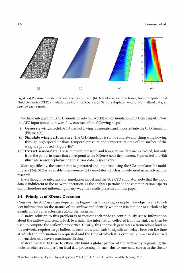
Fig. 4. (a) Pressure distribution over a wing’s surface. (b) Data of a single time-frame, from ComputationalFluid Dynamics (CFD) simulation, as input for XDense. (c) Sensors displacement; (d) Normalized data, asseen by each sensor.
We have integrated this CFD simulator into our workflow for simulation of XDense inputs. Now,the AFC input simulation workflow consists of the following steps:
(i) Generatewingmodel:A3Dmesh of awing is generated and imported into the CFD simulator(Figure 4(a));
(ii) Simulate wing performance: The CFD simulator is run to simulate a pitching wing flowingthrough high speed air flow. Temporal pressure and temperature data of the surface of thewing are produced. (Figure 4(b));
(iii) Extract sensor data: These temporal pressure and temperature data are extracted, but onlyfrom the points in space that correspond to the XDense node deployment. Figures 4(c) and 4(d)illustrate sensor deployment and sensor data, respectively.
More specifically, the sensor data is generated and imported using the SU2 simulator for multi-physics [24]. SU2 is a reliable open-source CFD simulator which is widely used in aerodynamicsresearch.
Even though we integrate our simulation model and the SU2 CFD simulator, note that the inputdata is indifferent to the network operation, as the analysis pertains to the communication aspectsonly. Therefore not influencing in any way the results presented in this paper.
2.4 Principles of XDense Operation
Consider the AFC use case depicted in Figure 1 as a working example. The objective is to col-lect information on the nature of the airflow and identify whether it is laminar or turbulent byquantifying its characteristics along the wingspan.A naive solution to this problem is to request each node to continuously sense information
about the airflow and send it back to a sink. The information collected from the sink can then beused to compute the airflow’s properties. Clearly, this approach generates a tremendous load onthe network, requires large buffers in each node, and leads to significant delays between the timeat which the information is requested and the time at which it is eventually processed (sensedinformation may have a maximum lifetime).Instead, we use XDense to efficiently build a global picture of the airflow by organizing the
nodes in clusters and perform local data processing. In each cluster, one node serves as the cluster
ACM Transactions on Cyber-Physical Systems, Vol. 1, No. 1, Article 1. Publication date: January 2018.

Extensive Analysis of a Real-Time Dense Wired Sensor Network Based on Traffic Shaping 1:7
(d)
(b)
(c)(a)
Input flow Output flow
Fig. 5. Example 45 × 45 network, with a single central sink. In this case, with nradius = 2. Application phases:(a) ϕ1 ś Sink requests data from cluster-heads; (b) ϕ2 ś Cluster heads in turn send a multicast request tonodes in their cluster; (c) ϕ3 ś Nodes send sensor data back to their respective cluster-head; (d) ϕ4 ś Clusterheads process received data and send result to sink.
head node. It performs data aggregation within its cluster and is responsible for processing (and/orcompressing) the data locally to send only meaningful information to the sink. Another exampleof utilization is to program the cluster heads to inform the sink only upon the occurrence ofmeaningful events (e.g., airflow changes from laminar to turbulent and conversely).
The routing protocols elected should ideally exploit the network topology to avoid congestion. Itis also required to define application protocols to allow coordination of clusters by the sink.
To tackle the challenge of analyzing and computing upper-bounds on the application executiontime and the buffer requirements of the nodes through distributed processing, XDense uses threeoperative principles: (1) the nodes are clustered and one node in each cluster (cluster head) is incharge of aggregating and pre-processing the data; (2) the execution of the application is dividedlogically in subsequent phases; (3) the network implements routing schemes which guaranteesspatial isolation between the clusters.
2.4.1 Clustering nodes. The reason for grouping the nodes into clusters is to reduce the load onthe network by performing in-cluster data pre-processing at the selected cluster heads. Our testedsolution implements non-overlapping łsquarež clusters ś the network topology being a 2D gridof X times Y nodes, all clusters are non-overlapping and of size nsize × nsize, with nsize ≤ X andnsize ≤ Y . nsize must be a positive odd number and the cluster head is the node located at the łcenteržof the square. The cluster size nsize is defined through the system parameter nradius that denotes themaximum distance from the cluster head to the farthest node in the cluster (considering rectilineardistance, a.k.a. Manhattan distance). Figure 5 shows a scenario with nradius = 2. Thus, the resultingtotal number of nodes in each cluster is a function of the nradius given by (2 × nradius + 1)
2.Nodes arbitrate their role on the network at run time (to act either as cluster head or normal
node). They do this on reception of a packet from the sink containing the packet origin and thenradius parameter. Each node then calculates, based on its position in the network relative to thesink, if it is supposed to act as a cluster head or as a normal node.
As discussed earlier, the purpose of local in-cluster processing is to extract high level aerodynamicinformation of the airflow, which is transmitted in a smaller number of packets (when compared tothe number of packets required to transmit the raw data). The pre-processing and compressionalgorithms to be used are application-specific and are not in the scope of this paper. We have though
ACM Transactions on Cyber-Physical Systems, Vol. 1, No. 1, Article 1. Publication date: January 2018.

1:8 J. Loureiro et al.
discussed application specific data processing issues in previous works (see [20] for a discussion onthis topic).
2.4.2 Executing application in phases. The execution of the application is logically divided intoa set of four consecutive phases ϕ1,ϕ2,ϕ3 and ϕ4. The first phase is started by the sink, when itrequests data from the cluster heads. Specifically, the four phases are:
• Phase ϕ1. The sink requests the cluster heads of all clusters to send the processed data;• Phase ϕ2. On receiving the request from the sink, the cluster heads in turn request the nodesof their respective clusters to send their data;• Phase ϕ3. Every node of each cluster transmits its sensed data to its cluster head;• Phase ϕ4. The cluster heads process the received data and transmit the result back to the sink.
Note that the clusters may not always be in sync with respect to the phase of their execution.The second phase (ϕ2) for instance, start in each cluster with a different time offset; This offsetbeing proportional to the distance between the cluster head of each cluster and the sink. We assumecluster heads’ clock are synchronized during ϕ1, at the time they receive the request from the sink.The same applies to sensor node’s clock, which are synchronized during ϕ2, at the time they receivethe request from their cluster head. That is, all nodes co-participating on a phase (in the samecluster) have a common time basis, which is an important assumption for the proposed heuristicsto work. We believe this is a reasonable assumption, since nodes synchronization point happenjust before synchronism is required, providing a momentary synchronism during a given phase,even when there is considerable clock skews between nodes.Despite their special role, the sink and cluster heads sense as any other node. The sink is the
only node to act as the gateway with the outside world and has a backhaul link (for example, awireless link). Figures 5(a) to 5(d) show the four phases in a chronological order.
2.4.3 Spatial isolation through routing schemes. The four phases described above require spatialisolation so that packets do not compete with each other for network resources when traversingit. We use the well-known dimension-order routing algorithms known as X-Y and Y-X routingprotocols [14]. In X-Y routing (resp, Y-X), packets are first routed along the X (resp, Y) dimensionand then along the Y (resp, X) dimension. These protocols always find the shortest path betweenthe source and destination nodes (again, in terms of the Manhattan distance) and are proven to bedeadlock-free [11].
Phases ϕ1 to ϕ3 use one of the following two routing algorithms, sometimes called Counterclock-wise Dimension Routing (see Figures 5(a)-(c)). The starting dimension (X or Y) depends on thequadrant in which the destination node is, relatively to the origin of the packet. For phase ϕ4 wepropose another routing protocol hereafter referred to as Shifted Clockwise Dimension Routing.This protocol adds an initial change in dimension on the first hop and then uses a regular clockwiserouting (see Figure 5(d)).
The nodes aligned with the sink are not part of any cluster. They provide an exclusive route forpackets of ϕ4, sent by the cluster head to the sink. This routing scheme results in flows from phaseϕ4 to travel orthogonal to the flows from phases ϕ1,ϕ2 and ϕ3 and therefore they do not competefor the same output port at any node on the way. This enables spatial isolation between the flowsfrom the different phases.
3 EXTENDING XDENSE WITH REAL-TIME APPLICATION CAPABILITIES
We endow XDense with real-time capabilities by shaping the traffic at every output port of every
node in the network. In simple terms, by controlling how and when packets are sent by each node,
ACM Transactions on Cyber-Physical Systems, Vol. 1, No. 1, Article 1. Publication date: January 2018.
Extensive Analysis of a Real-Time Dense Wired Sensor Network Based on Traffic Shaping 1:9
f1
f2
R TS f3
ND
Node 0510152025
051015TTS
TTS
Fig. 6. Traffic shaper example scenario: two input flows shaped by an intermediate node as an output flow.Parameters for the input flows are f1 = {O = 2.5, β = 1,σ = 10} and f2 = {O = 1, β = 1
5 ,σ = 3}. The resulting
flow is f3 = {O = 2, β = 12 ,σ = 13}.
we are able to compute the maximum buffer requirement and determine precise upper-bounds onthe application execution time.
3.1 Networking model
The real-time application deployed on the network is characterized by a set Φ = {ϕ1,ϕ2, . . . ,ϕn } ofn consecutive event-triggered phases (communication and processing primitives) that constitutethe logical part of the application execution. In this work, we assume n = 4 (as explained in theprevious section) but the approach can be extended to any arbitrary number n of phases. Everyphase ϕi ∈ Φ, with i ∈ [1,n], is characterized by a set Fi ofmi ≥ 1 communication traffic flowsexchanged between the nodes involved in phase ϕi . Each flow fi, j ∈ Fi , with j ∈ [1,mi ], consistingof one or more packets, has an unique source node from which the communication is initiated, andmay have multiple destination nodes. Formally, a flow fi, j is modeled as:
fi, j = {Oi, j , σi, j , βi, j } (1)
The offset Oi, j is a constant delay before the sending of the first packet of flow fi, j . The messagesize σi, j is the number of packets that are sent in each flow fi, j and the burstiness βi, j ∈ [0, 1]represents the rate at which those packets are released. A burstiness of 0 means that no packetsare transmitted, and a burstiness of x ∈ ]0, 1] means that a packet is transmitted every 1
xTTS.
These three parameters together describe a finite constant-rate flow with an initial offset. The flowparameters σ and β were conceived to couple the application sampling requirements with thecommunication model, in the sense that they allow modeling application scenarios with differentdata sampling requirements. A few example flows are illustrated below.
Example 3.1 (9 Degrees of Freedom (DOF) motion sensor). Consider a 9 DOF motion sensor whosedata has to be transmitted as nine separate packets in a single flow (one packet for each degree offreedom). In this case, we want the data to be transmitted together. Therefore, we set β = 1 withσ = 9 for that flow.
Example 3.2 (Pressure sampling). Consider a use-case in which ten samples of pressure data needto be transmitted, using one packet per sample. We are interested in having periodic sampling,equally distributed in time. By setting the burstiness to 1
5 for instance, one packet will be sent every
5 TTS. Therefore, for that flow we set β = 15 and σ = 10.
3.2 Shaping flows and traffic throughout the network
As discussed above, the sending of all packets by the source node of the corresponding flow f isdone according to its parameters (O,σ , β); these three parameters allow for a precise timing andsending rate at the source node of f . Note that for simplicity, we shall use hereafter the symbolf to denote a flow. We will mention the indexes i and j that indicate the phase and flow indexesrespectively only if necessary.
ACM Transactions on Cyber-Physical Systems, Vol. 1, No. 1, Article 1. Publication date: January 2018.

1:10 J. Loureiro et al.
Although the flows are shaped at their source, whenmultiple flows (say, f in1 , fin2 , . . . , f
ink) traverse
the network at the same time, pass through the same router, and compete for the same output port,the resulting output flow f out at that port is a superposition of all these competing flows. As such,f out may present an irregular packet transmission pattern and a rate that can no longer be modeledusing the three parameters (O,σ , β).
For example, let us look at Figure 6, which illustrates two input flows f in1 and f in2 competing for a
same output port of a node. Each of these flows f ink
starts at time Ok and has a duration defined as
ℓk =σkβk. That is, flow fk sends all its packets after ℓk TTS, at t = Ok + ℓk . In this example, thanks
to the traffic shaper TS, the interference of these two input flows lead to an output flow f out3 that isnot a superposition of the two input flows, but rather it preset deterministic patterns that can bemodeled using the three parameters (O,σ , β).That is, to make the network amenable to timing analysis, we shape the traffic at every output
port of every node and make it fit the linear model (O,σ , β). For that, we first identify the set ofinput flows f in
k(with k = 1, 2, . . .) at every output port of every node in the network, and based on
the respective parameters (Ok ,σk , βk ) of these flows, we compute the parameters (Oout,σ out, βout)that are used to shape the resulting output flow at that output port.In Figure 7, we present a more detailed example to illustrate how the traffic shaping is done.
Figure 7(a) shows packet arrivals curve S (t ) due to four incoming flows f in1 , fin2 , f
in3 and f in4 (see
Figure 7(b)). The arrival curve correspond to the incoming flows that define the number of packetsto be sent over time from the output port, that depends on the starting time and duration of all thecompeting input flows. Three possible resulting flows f out are computed and shown in Figure 7(c),each with its corresponding departure curve in Figure 7(a).The computation of (Oout,σ out, βout) is therefore performed at every output port of every node
in the network interactively, starting at the source node of every flow and iterating, one port atthe time, throughout the network until a shaper is defined for all the output ports. 3 We make twoimportant assumptions regarding the flows and their routing.Assumption 1. During phases ϕ3 and ϕ4, in every node, all the packets entering by a given
input port are assumed to exit through a single output port.Assumption 2. There are no circular dependency between the flows. For any output port, say
p1, the computation of the parameters of its traffic shaper requires each of its competing inputflows to be modeled already by the three parameters (O,σ , β). If any of these input flows, sayf ink, comes from the output port (say p2) of an upstream router, it is required that the parameters
(O ink,σ in
k, β in
k) of the shaper of that upstream output port p2 have been computed already. Similarly,
this requirement must be satisfied for all the input flows competing for p2, and interactively itmust be satisfied as well for all the output ports of the upstream routers till the traffic shaper at thesource nodes of all the interfering flows. Therefore, computing traffic shaping parameters is aniterative process that must be executed until (Oout,σ out, βout) is calculated for all nodes. In simpleterms, there cannot be a flow f1 competing for an output port with a flow f2 that competes for anoutput port with a flow f3, and so on until reaching a flow fk that competes for an output port withf1.Assuming no cyclic dependencies between the flows, the parameters (Oout,σ out, βout) of every
traffic shaper may be computed in many different ways for a same set of interfering input flows. Inthe next section, we propose three different methods of computation.
3Note that it has been proven in [35] that to calculate optimal shaping parameters in a multihop scenario can be computa-
tionally intractable, and thus finding optimal solution at runtime is not feasible.
ACM Transactions on Cyber-Physical Systems, Vol. 1, No. 1, Article 1. Publication date: January 2018.

Extensive Analysis of a Real-Time Dense Wired Sensor Network Based on Traffic Shaping 1:11
S(t)Min-OMax-SLQ
oLQoMin-O oMax-S
βMin-O
Time (t)
Packet
coun
t (n
)
βMax-S
p1
p2 p3
p4
p5
p6
p7
p8
f1 f2
f3 f4
(a)
(b)
Time (t)
βLQ
fMin-O
fMax-S
Time (t)
(c) fLQ
Fig. 7. Traffic shaping heuristics: (a) input, and output flows using the proposed heuristics; time-line showingoffset and duration of (b) arriving flows and (c) departure flows.
3.3 Shaping output traffic at a single output port
We propose three heuristics to compute the parameters (Oout,σ out, βout) of the shaper used at agiven output port. Let F in denote the set of input flows that compete for the output port underanalysis. Every f in
k∈ F in is characterized by the three parameters (O in
k,σ in
k, β in
k). For each f in
k∈ F in,
we define the function S ink(t ) as
S ink (t ) =
0 t ≤ O ink
β ink× (t −O in
k) O in
k< t < O in
k+ ℓk
σ ink
t ≥ O ink+ ℓk
(2)
Broadly speaking, every function S ink(t ) represents the number of packets sent by the flow f in
kat a
given time t (TTS). When t is earlier than the starting instant O inkof the flow, the function returns
0 since the flow has not sent a packet yet; For t larger than the finishing time of the flow (O ink+ ℓk ),
the function returns the total number σ ink
of packets sent by f ink, with ℓk being the duration of the
flow; Between the two bounds O inkand O in
k+ ℓk , the function increases steadily from 0 to σ in
kwith
a constant slope of β ink.
Let S (t ) =∑
f ink∈F in S ink (t ) be the sum of the functions S in
k(t ) of all the input flows f in
k. This
function S (t ) is depicted in Figure 7(a). Informally, S (t ) gives the number of packets that arrive at theconsidered input port in a time window of length t (TTS). We further denote by T = {t1, t2, . . . , tm }the finite set of time-instants (sorted in chronological order) corresponding to the discontinuitypoints of the function S (t ). These discontinuity points are denoted asp1,p2, . . . ,pm in Figure 7. Withthese new notations, we can introduce our three heuristics for the computation of the parameters(Oout,σ out, βout) of the shaper used at the analyzed output port.For a given shaper (Oout,σ out, βout) represented by a straight line Lout of slope βout and passing
through the point (Oout, 0), the vertical distance dvoutj between a point (tj , S (tj )) ∈ S (t ), ∀tj ∈ T ,
and the line Lout represents the number of packets being buffered at time t at that output port. Thehorizontal distance dhoutj between a point (tj , S (tj )) ∈ S (t ), ∀tj ∈ T and Lout represents the delay
ACM Transactions on Cyber-Physical Systems, Vol. 1, No. 1, Article 1. Publication date: January 2018.
1:12 J. Loureiro et al.
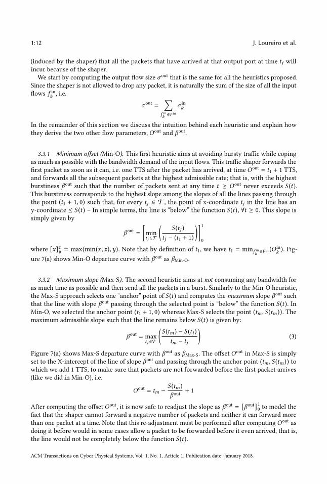
(induced by the shaper) that all the packets that have arrived at that output port at time tj willincur because of the shaper.
We start by computing the output flow size σ out that is the same for all the heuristics proposed.Since the shaper is not allowed to drop any packet, it is naturally the sum of the size of all the inputflows f in
k, i.e.
σ out=
∑
f ink∈F in
σ ink
In the remainder of this section we discuss the intuition behind each heuristic and explain howthey derive the two other flow parameters, Oout and βout.
3.3.1 Minimum offset (Min-O). This first heuristic aims at avoiding bursty traffic while copingas much as possible with the bandwidth demand of the input flows. This traffic shaper forwards thefirst packet as soon as it can, i.e. one TTS after the packet has arrived, at time Oout
= t1 + 1 TTS,and forwards all the subsequent packets at the highest admissible rate; that is, with the highestburstiness βout such that the number of packets sent at any time t ≥ Oout never exceeds S (t ).This burstiness corresponds to the highest slope among the slopes of all the lines passing throughthe point (t1 + 1, 0) such that, for every tj ∈ T , the point of x-coordinate tj in the line has any-coordinate ≤ S (t ) ś In simple terms, the line is łbelowž the function S (t ), ∀t ≥ 0. This slope issimply given by
βout =
[mintj ∈T
(
S (tj )
tj − (t1 + 1)
)]1
0
where [x]zy = max(min(x , z),y). Note that by definition of t1, we have t1 = minf ink∈F in (O in
k). Fig-
ure 7(a) shows Min-O departure curve with βout as βMin-O.
3.3.2 Maximum slope (Max-S). The second heuristic aims at not consuming any bandwidth foras much time as possible and then send all the packets in a burst. Similarly to the Min-O heuristic,the Max-S approach selects one łanchorž point of S (t ) and computes the maximum slope βout suchthat the line with slope βout passing through the selected point is łbelowž the function S (t ). InMin-O, we selected the anchor point (t1 + 1, 0) whereas Max-S selects the point (tm , S (tm )). Themaximum admissible slope such that the line remains below S (t ) is given by:
βout = maxtj ∈T
(
S (tm ) − S (tj )
tm − tj
)
(3)
Figure 7(a) shows Max-S departure curve with βout as βMax-S. The offset Oout in Max-S is simply
set to the X-intercept of the line of slope βout and passing through the anchor point (tm , S (tm )) towhich we add 1 TTS, to make sure that packets are not forwarded before the first packet arrives(like we did in Min-O), i.e.
Oout= tm −
S (tm )
βout+ 1
After computing the offset Oout, it is now safe to readjust the slope as βout =[
βout]10 to model the
fact that the shaper cannot forward a negative number of packets and neither it can forward morethan one packet at a time. Note that this re-adjustment must be performed after computing Oout asdoing it before would in some cases allow a packet to be forwarded before it even arrived, that is,the line would not be completely below the function S (t ).
ACM Transactions on Cyber-Physical Systems, Vol. 1, No. 1, Article 1. Publication date: January 2018.

Extensive Analysis of a Real-Time Dense Wired Sensor Network Based on Traffic Shaping 1:13
Figure 7(a) shows the departure line of Max-S, initially calculated with a slope > 1 as a resultof Equation 3. That slope is then adjusted to βout = 1 as depicted on that Figure. As seen, afteradjusting its slope, the line corresponding to the parameters of the Max-S traffic shaper does notintersect with the function S (t ) ś It seems to be łtoo much shifted to the rightž. An easy patch toreduce this gap between S (t ) and the shaper is to set its offset to the minimum offset such that theline remains below all the points of S (t ). That is,
Oout= min
t ≥0
t such that βout ≤ min
tj ∈T
tj>t
(
S (t ) − S (tj )
t − tj
)(4)
Note that this value of Oout can be computed easily by positioning the line of slope βout on everypoint (tj , S (tj )), ∀tj ∈ T , and retaining the maximum X-intercept of all these lines.
3.3.3 Least-square regression (LQ). The intuition behind this third heuristic is to minimize boththe queue size and the delay by finding the line Lout that minimizes the distance between everypoint (tj , S (tj )) ∈ S (t ), ∀tj ∈ T and Lout. This line is commonly known as the regression line of thepoints (tj , S (tj )) ∈ S (t ). Using the least-squares method, which is the most common method forfitting a regression line, the slope of that line is given by
βout = r ×
√
1
m
∑
tj ∈T
(S (tj ) − S̄ )2
√
1
m
∑
tj ∈T
(tj − t̄ )2
(5)
where
t̄ =
1
m
∑
tj ∈T
tj
S̄ =
1
m
∑
tj ∈T
S (tj )
and r is the correlation coefficient computed as
r =
∑
tj ∈T
(tj − t̄ ) (S (tj ) − S̄ )
√
∑
tj ∈T
(tj − t̄ )2∑
tj ∈T
(S (tj ) − S̄ )2
Once we have computed the slope, we choose the smallest offset Oout such that the line of slopeβout and passing through (Oout, 0) is never above any point (t , S (t )), ∀t ≥ 0. This is done usingEquation 4.
3.4 Worst-case per-hop delays and maximum queue sizes
Having stated the heuristics, we can now apply them to all the phases of the application. Weperform this in a hop-by-hop strategy, starting from the output ports of the nodes for which theparameters (O in
k,σ in
k, β in
k) of all the interfering flows f in
kare known. For each such output port, the
resulting output flow f out is shaped using the same model (Oout,σ out, βout) that is then propagatedas the input flow in the next hop. The process continues until the parameters of the shaper of
ACM Transactions on Cyber-Physical Systems, Vol. 1, No. 1, Article 1. Publication date: January 2018.

1:14 J. Loureiro et al.
every output port of all the nodes of the network are defined (the output ports that no flows evertraverse and that are thus unused are naturally ignored). As mentioned earlier, we assume thatthere are no cyclic dependencies between the flows at any output port, which implies that theprocess eventually terminates.
After that step, we can now compute at each output port the maximum transmission delay causedby its traffic shaper (Oout,σ out, βout), as well as its maximum queue size. To ease the explanation,we shall use the same visual representation as that used in the previous section for the shaper andthe function S (t ). The shaper is represented by a straight line of slope βout that intersects with thex-axis at the point (Oout, 0). We denote this line Lout and write its equation as
Lout (t ) = βoutt − βoutOout (6)
We define S (t ) as in the previous section and keep the notations T = {t1, t2, . . . , tm } to express thefinite set of time-instants (sorted in chronological order) corresponding to the discontinuity pointsof the function S (t ).
As explained previously, the number of packets buffered at the output port at any time-instant tis given by the vertical distance dvoutj between the point (t , S (t )) and the point (t ,Lout (t )) on the
line Lout. This vertical distance is simply equal to
dvoutj = S (t ) − Lout (t )
and thus the maximum number MaxQueue of packets buffered at that output port is given by
MaxQueue = maxt ≥0
(
S (t ) − Lout (t ))
Since S (t ) is a continuous piecewise function for which every sub-function is linear, it can easilybe showed that the maximum of the previous equation can be found by looking only at thetime-instants tj ∈ T rather than at all t ≥ 0, i.e.,
MaxQueue = maxtj ∈T
(
S (tj ) − Lout (tj )
)
(7)
This holds true because every sub-function of S (t ) is a segment that is either:
• parallel to Lout. In this case, all the points on that segment are at the same distance from Lout,including its two extremities that are discontinuity points with an x-coordinate included inT .• converging towards Lout. In this case, the leftmost point on the segment (whose x-coordinateis an instant tj ∈ T ) is the furthest to Lout.• diverging from Lout. In this case, the rightmost point on the segment (whose x-coordinate isan instant tj ∈ T ) is the furthest to Lout.
Similarly, the transmission delay at any time-instant t is given by the horizontal distance dhoutj
between the point (t , S (t )) and the point of y-coordinate S (t ) on the line Lout. According to Equa-tion 6, that point of y-coordinate S (t ) ∈ Lout has an x-coordinate x such that S (t ) = βoutx − βoutOout
and thus x =S (t )β out +O
out. The horizontal distance is then simply given by:
dhoutj =S (t )
βout+Oout − t
and thus the maximum delay MaxDelay at that output port is:
MaxDelay = maxt ≥0
(
S (t )
βout+Oout − t
)
ACM Transactions on Cyber-Physical Systems, Vol. 1, No. 1, Article 1. Publication date: January 2018.
Extensive Analysis of a Real-Time Dense Wired Sensor Network Based on Traffic Shaping 1:15
0 5 10 15 20 25 30Transmission time slot (TTS)
0
2
4
6
8
Cum
ulat
ive
pack
et c
ount
SIMMin-ODelayQueue
(a)
0 5 10 15 20 25 30Transmission time slot (TTS)
0
2
4
6
8
Cum
ulat
ive
pack
et c
ount
SIMMax-SDelayQueue
(b)
0 5 10 15 20 25 30Transmission time slot (TTS)
0
2
4
6
8
Cum
ulat
ive
pack
et c
ount
SIMLQDelayQueue
(c)
Fig. 8. Cumulative arrival/departure curves for a single node, using (a)Min-O, (b)Max-S and (c) LQ heuristics.
For the same reasons as those mentioned for MaxQueue, the maximum delay MaxDelay can becomputed by looking only at the points tj ∈ T , i.e.,
MaxDelay = maxtj ∈T
(
S (tj )
βout+Oout − tj
)
(8)
Note that the transmission delay is an interesting parameter to analyze the end-to-end delayor per-hop delays of individual packets. However, in this paper we rather focus on estimatingupper-bounds on the execution time of the phases and thus of the overall real-time application.To compute the execution time of a given phase, we must know exactly when the phase start
and when it ends. However, phases may overlap in time and happen simultaneously. For instance,for the application scenario considered in this paper, a cluster head located close to the sink mayenter phase ϕ2 long before a cluster head that is far from the sink (since it receives the request fromphase ϕ1 sooner). For simplicity, we assume in this work that a phase ends when a given node hasreceived all the packets sent to it. For example, the time at which all the cluster heads have receivedtheir requested data marks the end of phase ϕ3 and the time at which the sink has received all theprocessed data marks the end of phase ϕ4. As such, we compute the execution time of a phase asthe relative time-instant at which all the four input flows of that given node ś a cluster head forphase ϕ3 and the sink for phase ϕ4 ś terminate, i.e. the four flows coming from the north, south,east, and west input ports of that node. The execution time of a phase is thus given by
ExecTime = maxcard∈[↑,↓,→,←]
(
O in+
σ in
β in
)
(9)
where for each cardinal direction ↑, ↓, →, and ← (north, south, east, and west), the flow f in
characterized by (O in,σ in, β in) is the input flow coming from that cardinal direction.
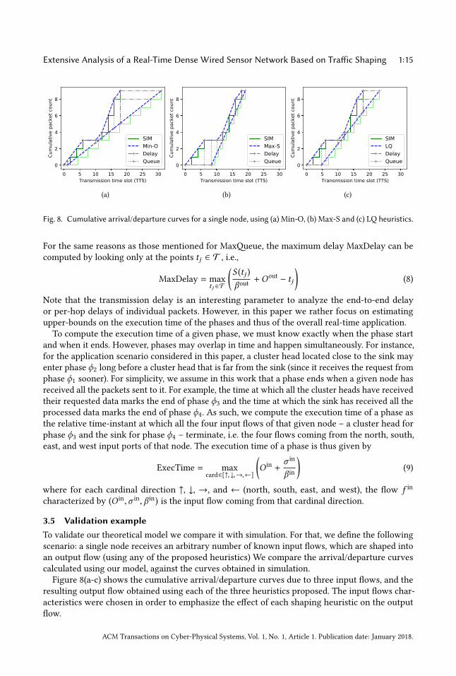
3.5 Validation example
To validate our theoretical model we compare it with simulation. For that, we define the followingscenario: a single node receives an arbitrary number of known input flows, which are shaped intoan output flow (using any of the proposed heuristics) We compare the arrival/departure curvescalculated using our model, against the curves obtained in simulation.Figure 8(a-c) shows the cumulative arrival/departure curves due to three input flows, and the
resulting output flow obtained using each of the three heuristics proposed. The input flows char-acteristics were chosen in order to emphasize the effect of each shaping heuristic on the outputflow.
ACM Transactions on Cyber-Physical Systems, Vol. 1, No. 1, Article 1. Publication date: January 2018.

1:16 J. Loureiro et al.
We use the same input flows in all three scenarios, which are Fx = [f in1 , fin2 , f
in3 ], where f in1 =
{O = 0,σ = 3, β = 0.5}, f in2 = {O = 10,σ = 3, β = 0.5} and f in3 = {O = 12,σ = 3, β = 0.5}. Theresulting output flows are different for each heuristic, which are f out
Min−O= {O = 1,σ = 9, β = 0.3},
f outMax−S
= {O = 8.2,σ = 9, β = 0.83} and f outLQ= {O = 4.8,σ = 9, β = 0.49}.
The arrival curves obtained through simulation (common to the three cases) is a stair functionthat presents the superposition of all the arriving flows. Because the output flow is shaped, thecorresponding departure curve is a homogeneous stair function. As expected, the arrival/departurecurves calculated using our model precede the simulated ones in every point. It also shows thequeue size and delay calculated at every point in which the arrival and/or departure curves start,finish or change its slope.
For the given Fx , from Figure 8(a), Min-O performs badly compared to the other heuristics, as itadds large delays between the arrivals and departures, which leads to equally large queues andlong execution time. We notice from Figure 8(b) that the departure curve obtained with Max-Sapproaches maximally the arrival curve at its tip (1 TTS far), leading to the optimal execution timewith the cost of larger queues from 0 to 10 TTS. On the other hand, LQ heuristic leads to smallerqueues, with a slightly longer execution time.Although these results provide an intuition on the trade-offs between the heuristics proposed,
they do not depict the results of multi-hop communication, in which case the effects may differ.Therefore, a more complete evaluation is provided in the next section to understand how eachheuristic performs through multiple hops.
4 EVALUATION OF TRAFFIC SHAPING HEURISTICS
Application use-case: To evaluate the proposed heuristics, we consider the application scenariointroduced in Section 2. Remember that the execution of this application is divided logically infour consecutive phases ϕ1,ϕ2,ϕ3 and ϕ4. In the first phase ϕ1, the unique sink node requests allthe cluster heads to send their data; in phase ϕ2, the cluster heads performs another request to allthe nodes of their respective cluster; in phase ϕ3, the nodes reply to the cluster heads by sendingthem the sensed data; and in phase ϕ4, the cluster heads process the data received and transmitthe result back to the sink. Since there is no network congestion in phases ϕ1 and ϕ2 ś because allthe packets sent from the sink to the cluster heads and then from the cluster heads to the sensingnodes have their own private route to their destination ś these two phases are neither affectedby a modification of the cluster size, nor by changing the number of clusters, nor by alteringthe burstiness of the flows generated during phases ϕ3 and ϕ4. We shall therefore focus only onphases ϕ3 and ϕ4 in which network congestion does occur and for which a modification of theaforementioned parameters has an impact on the performance.Network setup: The network is organized as a square grid of 45 × 45 = 2025 nodes with an
unique sink located at the center of the grid. Figure 5 depicts a closeup on the sink. In that figurewe can also see the overall cluster organization, the routes taken by the flows in the differentphases and the central row and central column of nodes in the middle that are dedicated only tothe communication between the cluster heads and the sink. Based on an integer parameter nradiusthat we vary in our experiments, we define every cluster as a square grid of (2nradius + 1)
2 nodeswith the cluster head at the center of the grid. As such, nradius defines both the cluster size andthe number of clusters (the smaller the clusters, the more clusters in the network, and reversely).Because of our routing algorithms and network symmetry assumptions (position of sink in thecenter of the network and cluster-head in the center of their cluster), the workload observed ineach quadrant around the sink or cluster-heads will be identical. This makes it sufficient to analyzea single quadrant of the network or cluster.
ACM Transactions on Cyber-Physical Systems, Vol. 1, No. 1, Article 1. Publication date: January 2018.

Extensive Analysis of a Real-Time Dense Wired Sensor Network Based on Traffic Shaping 1:17
Shaping heuristics: We evaluate the performance of the three proposed heuristics Min-O,Max-S, and LQ against the performance of a cycle-accurate network simulator that we call BE. Thesimulator does not implement any traffic shaper and thus it delivers the best effort (BE) performanceoverall.Simulator: The simulator consists of a module for XDense on top of Network-Simulator-3
(NS-3). It is scalable to simulate very large network deployment scenarios with low computationalcost. This is because we use packets, routing algorithms and addressing schemes with low overhead,tailored to this kind of network.The general nature of the design and implementation of configurable links, packets, communi-
cation ports, router and applications, also makes our module suitable to other 2D mesh networkarchitectures as well (NoCs for example). This is because the different abstraction levels can beimplemented independently, as a set of intermediate models, each one with its specific objectives.For example, the traffic shapers theorized in this work were actually implemented in our simulatoras an independent application layer, so we could study its practical viability, and for debuggingpurposes. 4
Evaluation criteria and methodology: For each of the three heuristics Min-O, Max-S, LQ, weevaluate the maximum queue sizes and the end-to-end execution time of the phases ϕ3 and ϕ4. ForBE, maximum queue sizes and phases execution time are measured in the simulator. We do so fordifferent cluster sizes, flow burstiness and network load distribution. Because there is no sourceof nondeterminism in our simulation model, each runs gives the exact same results for the sameinput parameters. Thus, we are only required to run our experiments once for each scenario, for aslong as all four phases last.
To understand the impact of varying the network load, we analyze both homogeneous and het-erogeneous flow scenarios in phases ϕ3 and ϕ4 (that is, the phases when the actual data transmissionhappens). We define a homogeneous flow scenario as one in which all nodes generate flows withequal burstiness and message size. A scenario with random message sizes and burstiness is definedas a heterogeneous flow scenario.
We analyze the homogeneous scenario by varying the burstiness β of flows from phases ϕ3 andϕ4 from 0.02 to 1 by step of 0.02, for different cluster sizes.
The message size σ differs for each phase. For phases ϕ1 and ϕ2, a single packet is generatedat the sink and cluster head (σ = 1). In phase ϕ3, each node outputs a flow with message sizeσ = 4. At the end of ϕ3, the cluster head receives in total four packets per each node on its cluster.Subsequently, each cluster head outputs a flow with message size σ , as the sum of all these packetsplus 4 packets of its own sensed data, times ⌈1 − CR⌉. The term CR aims at reproducing the effectof data compression by the cluster head. For this work we define this as a fixed value equal toCR = 80%, which was shown in previous work [20] to be a reasonable ratio in some air flowscenarios. The number of packets originated by each cluster vary with cluster size, whereas thenumber of clusters is inversely proportional to the cluster size. This trade off has a compensatoryeffect on the overall number of packets transmitted to the sink.
In the heterogeneous flow scenario, flows generated at phases ϕ3 and ϕ4 have random messagesizes. We use a uniform distribution function with σ = rand (0, 10) and burstiness β = rand (0.02, 1).A message size of zero signifies that a node does not have an output flow.
In our results, we compare the performance of both heterogeneous and homogeneous scenarios.In order to do this fairly, we guarantee that for both homogeneous (HO) and heterogeneous (HE)network load distribution, the sum of burstiness of all flows, as well as the sum of all message sizes,
4The simulator source code used in the simulation this paper for the simulator, pre and post processing tools, example
scenarios and implementation of the traffic shaping heuristics are available at: https://bitbucket.org/joaofl/noc
ACM Transactions on Cyber-Physical Systems, Vol. 1, No. 1, Article 1. Publication date: January 2018.

1:18 J. Loureiro et al.
0.0 0.2 0.4 0.6 0.8 1.0Burstiness ( )
0
10
20
30
40
Max
que
ue si
ze
Min-OMax-SLQBE
(a) ϕ3, nradius = 1
0.0 0.2 0.4 0.6 0.8 1.0Burstiness ( )
0
10
20
30
40
Max
que
ue si
ze
Min-OMax-SLQBE
(b) ϕ3, nradius = 3
0.0 0.2 0.4 0.6 0.8 1.0Burstiness ( )
0
10
20
30
40
Max
que
ue si
ze
Min-OMax-SLQBE
(c) ϕ3, nradius = 5
0.0 0.2 0.4 0.6 0.8 1.0Burstiness ( )
0
10
20
30
40
Max
que
ue si
ze
Min-OMax-SLQBE
(d) ϕ4, nradius = 1
0.0 0.2 0.4 0.6 0.8 1.0Burstiness ( )
0
10
20
30
40
Max
que
ue si
ze
Min-OMax-SLQBE
(e) ϕ4, nradius = 3
0.0 0.2 0.4 0.6 0.8 1.0Burstiness ( )
0
10
20
30
40
Max
que
ue si
ze Min-OMax-SLQBE
(f) ϕ4, nradius = 5
Fig. 9. Homogeneous flow scenario: Maximum queue size for traffic shaping heuristics against simulation.Results are for phases ϕ3 and ϕ4 and nradius set to 1, 3 and 5.
(a) BE, ϕ4, nradius = 5 (b) LQ, ϕ4, nradius = 5
Cluster head
Sink
Cluster
Fig. 10. Queue size density map of the top-right quadrant of the network (17×7 nodes), for heuristics (a) LQand (b) BE. X and Y axis are nodes coordinates relative to the sink.
are equal. That is,∑
βHO=
∑
βHE and∑
σHO=
∑
σHE . This guarantees that the total networkload remains the same for both scenarios, even if individual load distribution varies.
For both scenarios, the offset remains the same; and equal to their distance from the sink/clusterhead (since it is meant to model the minimum time required for a node to reply to a request).
4.1 Maximum queue size with homogeneous load distribution
For each of the three heuristics Min-O, Max-S and LQ, we first derive the parameters (O,σ , β ) ofall the traffic shapers in the network. Then we use Equation 7 on every shaper to compute the
ACM Transactions on Cyber-Physical Systems, Vol. 1, No. 1, Article 1. Publication date: January 2018.

Extensive Analysis of a Real-Time Dense Wired Sensor Network Based on Traffic Shaping 1:19
0.0 0.2 0.4 0.6 0.8 1.0Burstiness ( )
0.0
0.2
0.4
0.6
0.8
1.0
Link
utiliz
atio
n
Min-OMax-SLQBE
(a) ϕ3, nradius = 1
0.0 0.2 0.4 0.6 0.8 1.0Burstiness ( )
0.0
0.2
0.4
0.6
0.8
1.0
Link
utiliz
atio
n
Min-OMax-SLQBE
(b) ϕ3, nradius = 3
0.0 0.2 0.4 0.6 0.8 1.0Burstiness ( )
0.0
0.2
0.4
0.6
0.8
1.0
Link
utiliz
atio
n
Min-OMax-SLQBE
(c) ϕ3, nradius = 5
0.0 0.2 0.4 0.6 0.8 1.0Burstiness ( )
0.0
0.2
0.4
0.6
0.8
1.0
Link
utiliz
atio
n
Min-OMax-SLQBE
(d) ϕ4, nradius = 1
0.0 0.2 0.4 0.6 0.8 1.0Burstiness ( )
0.0
0.2
0.4
0.6
0.8
1.0
Link
utiliz
atio
n
Min-OMax-SLQBE
(e) ϕ4, nradius = 3
0.0 0.2 0.4 0.6 0.8 1.0Burstiness ( )
0.0
0.2
0.4
0.6
0.8
1.0
Link
utiliz
atio
n
Min-OMax-SLQBE
(f) ϕ4, nradius = 5
Fig. 11. Homogeneous flow scenario: Link utilization for traffic shaping heuristics against simulation. Resultsare for phases ϕ3 and ϕ4 and nradius set to 1, 3 and 5.
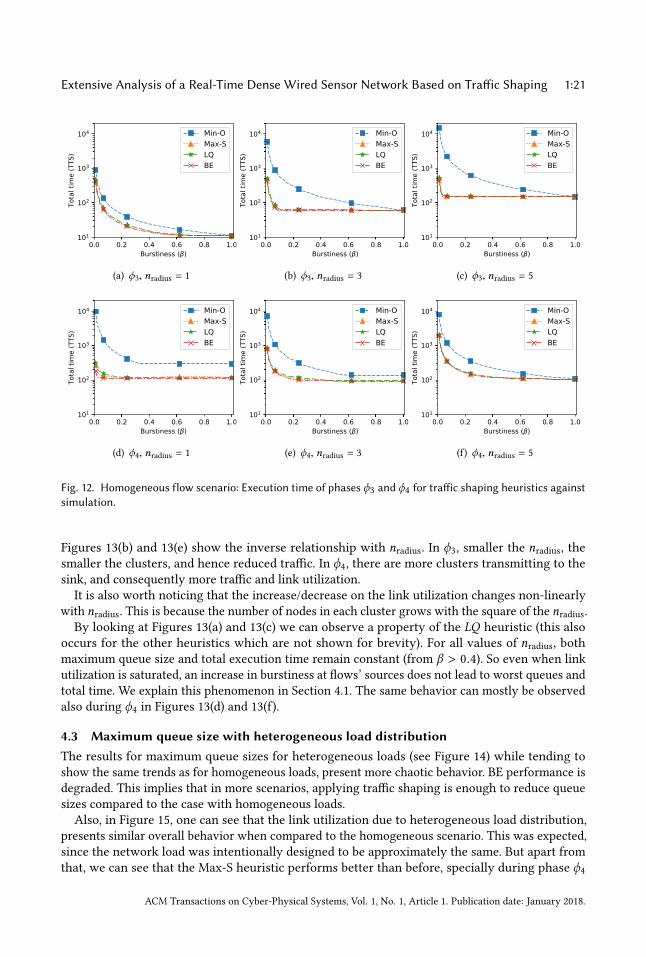
maximum queue size of the corresponding node and finally, we retain the maximum queue size ofall the nodes in the network.As we can see in Figures 9(a) and 9(b), in phase ϕ3 the queues are smaller for smaller clusters
(nradius). This is expected since smaller clusters contain less nodes and therefore there are lesspackets exchanged within each cluster, and thus less congestion. The opposite scenario would beexpected for phase ϕ4 since using smaller clusters means more clusters in the network, and thusmore cluster heads transmitting packets to the sink. Yet, this is not observed in Figure 9(d) and 9(e).That is, smaller clusters do not imply longer queues. The reason for this counter-intuitive result canbe unveiled by looking at the utilization of the four input links of the sink.
We define the link utilization as the average utilization of a given link of a node during a givenphase. It is calculated as the number of packets sent on that link in a given phase (here, phase ϕ4)divided by the time (number of TTS) it takes for all those packets to traverse it. An utilization of 1means that the link is never idle during the considered phase whereas an utilization of 0 means thatthe link is not used. As seen in Figure 11(d), smaller clusters yield a better utilization of the inputlinks of the sink. This is because the sum of packets sent to the sink does not depend only on thecluster size. With more (and smaller) clusters, there will be more clusters and more cluster-headstransmitting to the sink from shorter distances. Thus, its input links will spent less time idle waitingfor the packets to arrive from longer distances. In other words, with fewer (but bigger) clusters,cluster heads are farther from the sink and thus its input links spend more time idle waiting forthe packets to traverse the intermediate hops. Greater utilization, for the same number of packets
ACM Transactions on Cyber-Physical Systems, Vol. 1, No. 1, Article 1. Publication date: January 2018.

1:20 J. Loureiro et al.
received by the sink, shows that there is less congestion in the network and thus smaller queue atindividual hops.
It is worth noticing that in some scenarios, the maximum queue size obtained when using trafficshaping is smaller than the maximum queue size without traffic shaping. This is experienced forexample in ϕ4 for nradius = 3 and 5, shown in Figure 9(e) and 9(f), for β ∈ [0.4, 0.6]. In this window,the maximum queue size of Max-S and LQ are smaller than that of BE. This result is due to the offsetO imposed by the traffic shapers in the initial hops. In these cases, the offsets act on distributing intime the load on the network, and thus decreasing the maximum congestion.However, in cases with lower link utilization and burstiness, BE yields shorter queue sizes. In
these cases the network is underutilized, such that BE still does not lead to excessive load on thenetwork. On the other hand, performing traffic shaping imputes on unnecessary buffering by nodes,and consequently greater queues.The aforementioned effect is shown in Figure 10. It shows the queue size density map of the
top-right quadrant of the network, with nradius = 5. The sink is located at the bottom-left corner.Flows are routed using shifted clockwise routing as previously shown in Figure 5; hence, rightto left in this map. The left most nodes in the network are usually where the bottleneck happens.Using BE for example, in Figure 10(a), the node located at coordinates (x ,y) = (0, 5) gets up to 18packets queued, since it is located at a conjunction of flows coming from cluster heads on its rightand top. Because of the offset O calculated using LQ, we can see from Figure 10(b) that by shapingand queuing the flows originating at the right side of the network (by the node located at (6, 5))has the effect of delaying the reception of those packets by the left most node located at (0, 5);Thus, reducing the maximum queue size at the nodes aligned with the sink. Comparatively, from18 packets using BE, to 13 using LQ.
Another interesting observation occurs during ϕ4 for the method Min-O. The maximum queuesize gets smaller with increased burstiness. This is very counter-intuitive since we would expect thatby injecting more traffic in the network, the congestion would increase. However, this phenomenacan be easily explained mathematically: it is due to the way the method Min-O is defined. Lookingat Figure 7, the flows duration defined as σ
βare longer for lower burstiness β and thus for low
values of β , the first points ∈ T (depicted by p1, p2, etc.) are farther from the origin. Since Min-Oselects a point close to the origin as łanchorž point, its slope must be small so that the line remainsbelow the function S (t ). With a low slope, it is likely that the vertical distance between the functionS (t ) and the line will be high (in particular if S (t ) increases quickly). These phenomena can beobserved, to a limited extent, in Figure 7.
4.2 Phase execution time for homogeneous load distribution
We compare the execution time of the phases ϕ3 and ϕ4 in Figure 12, again for the cluster sizesdefined by nradius = 1, 3 and 5 and varying the burstiness of the initial flows from 0.02 to 1 by stepof 0.02. The execution times are computed by using Equation 9. As seen in all graphics of Figure 12,increasing the burstiness considerably reduces the execution time of the phases (note that theplots are in logarithmic scale) which remains constant after a point. This point is reached onlyfor high burstiness in Figure 12(a) whereas it is reached almost immediately in Figure 12(b). Thisthreshold beyond which the execution time cannot be further reduced can be explained by lookingat the utilization of input link of cluster heads (for phase ϕ3) and the sink (for phase ϕ4). Thosethresholds correspond to specific values of the burstiness for which the links saturate and therefore,any further increase in burstiness only results in longer queues but not in reduced execution time.
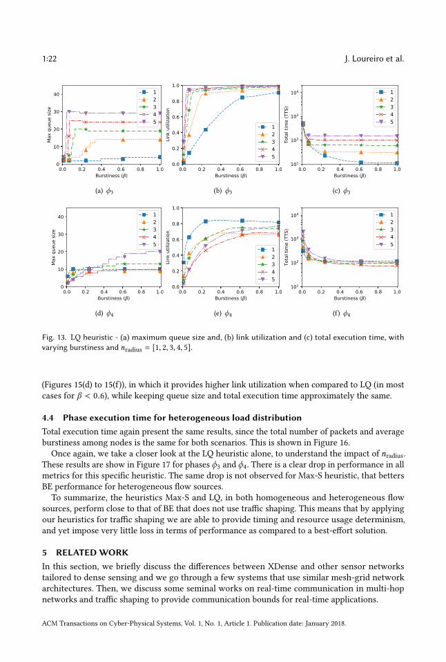
From the above results, we observe that the LQ heuristic performs better overall. We vary nradiusfrom 1 to 5, with β varying as before, for both ϕ3 and ϕ4. The results are shown in Figure 13.
ACM Transactions on Cyber-Physical Systems, Vol. 1, No. 1, Article 1. Publication date: January 2018.
Extensive Analysis of a Real-Time Dense Wired Sensor Network Based on Traffic Shaping 1:21
0.0 0.2 0.4 0.6 0.8 1.0Burstiness ( )
101
102
103
104
Tota
l tim
e (T
TS)
Min-OMax-SLQBE
(a) ϕ3, nradius = 1
0.0 0.2 0.4 0.6 0.8 1.0Burstiness ( )
101
102
103
104
Tota
l tim
e (T
TS)
Min-OMax-SLQBE
(b) ϕ3, nradius = 3
0.0 0.2 0.4 0.6 0.8 1.0Burstiness ( )
101
102
103
104
Tota
l tim
e (T
TS)
Min-OMax-SLQBE
(c) ϕ3, nradius = 5
0.0 0.2 0.4 0.6 0.8 1.0Burstiness ( )
101
102
103
104
Tota
l tim
e (T
TS)
Min-OMax-SLQBE
(d) ϕ4, nradius = 1
0.0 0.2 0.4 0.6 0.8 1.0Burstiness ( )
101
102
103
104
Tota
l tim
e (T
TS)
Min-OMax-SLQBE
(e) ϕ4, nradius = 3
0.0 0.2 0.4 0.6 0.8 1.0Burstiness ( )
101
102
103
104
Tota
l tim
e (T
TS)
Min-OMax-SLQBE
(f) ϕ4, nradius = 5
Fig. 12. Homogeneous flow scenario: Execution time of phases ϕ3 and ϕ4 for traffic shaping heuristics againstsimulation.
Figures 13(b) and 13(e) show the inverse relationship with nradius. In ϕ3, smaller the nradius, thesmaller the clusters, and hence reduced traffic. In ϕ4, there are more clusters transmitting to thesink, and consequently more traffic and link utilization.It is also worth noticing that the increase/decrease on the link utilization changes non-linearly
with nradius. This is because the number of nodes in each cluster grows with the square of the nradius.By looking at Figures 13(a) and 13(c) we can observe a property of the LQ heuristic (this also
occurs for the other heuristics which are not shown for brevity). For all values of nradius, bothmaximum queue size and total execution time remain constant (from β > 0.4). So even when linkutilization is saturated, an increase in burstiness at flows’ sources does not lead to worst queues andtotal time. We explain this phenomenon in Section 4.1. The same behavior can mostly be observedalso during ϕ4 in Figures 13(d) and 13(f).
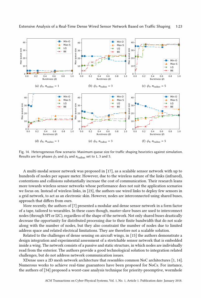
4.3 Maximum queue size with heterogeneous load distribution
The results for maximum queue sizes for heterogeneous loads (see Figure 14) while tending toshow the same trends as for homogeneous loads, present more chaotic behavior. BE performance isdegraded. This implies that in more scenarios, applying traffic shaping is enough to reduce queuesizes compared to the case with homogeneous loads.Also, in Figure 15, one can see that the link utilization due to heterogeneous load distribution,
presents similar overall behavior when compared to the homogeneous scenario. This was expected,since the network load was intentionally designed to be approximately the same. But apart fromthat, we can see that the Max-S heuristic performs better than before, specially during phase ϕ4
ACM Transactions on Cyber-Physical Systems, Vol. 1, No. 1, Article 1. Publication date: January 2018.
1:22 J. Loureiro et al.
0.0 0.2 0.4 0.6 0.8 1.0Burstiness ( )
0
10
20
30
40
Max
que
ue si
ze
12345
(a) ϕ3
0.0 0.2 0.4 0.6 0.8 1.0Burstiness ( )
0.0
0.2
0.4
0.6
0.8
1.0
Link
utiliz
atio
n
12345
(b) ϕ3
0.0 0.2 0.4 0.6 0.8 1.0Burstiness ( )
101
102
103
104
Tota
l tim
e (T
TS)
12345
(c) ϕ3
0.0 0.2 0.4 0.6 0.8 1.0Burstiness ( )
0
10
20
30
40
Max
que
ue si
ze
12345
(d) ϕ4
0.0 0.2 0.4 0.6 0.8 1.0Burstiness ( )
0.0
0.2
0.4
0.6
0.8
1.0
Link
utiliz
atio
n
12345
(e) ϕ4
0.0 0.2 0.4 0.6 0.8 1.0Burstiness ( )
101
102
103
104
Tota
l tim
e (T
TS)
12345
(f) ϕ4
Fig. 13. LQ heuristic - (a) maximum queue size and, (b) link utilization and (c) total execution time, withvarying burstiness and nradius = [1, 2, 3, 4, 5].
(Figures 15(d) to 15(f)), in which it provides higher link utilization when compared to LQ (in mostcases for β < 0.6), while keeping queue size and total execution time approximately the same.
4.4 Phase execution time for heterogeneous load distribution
Total execution time again present the same results, since the total number of packets and averageburstiness among nodes is the same for both scenarios. This is shown in Figure 16.Once again, we take a closer look at the LQ heuristic alone, to understand the impact of nradius.
These results are show in Figure 17 for phases ϕ3 and ϕ4. There is a clear drop in performance in allmetrics for this specific heuristic. The same drop is not observed for Max-S heuristic, that bettersBE performance for heterogeneous flow sources.To summarize, the heuristics Max-S and LQ, in both homogeneous and heterogeneous flow
sources, perform close to that of BE that does not use traffic shaping. This means that by applyingour heuristics for traffic shaping we are able to provide timing and resource usage determinism,and yet impose very little loss in terms of performance as compared to a best-effort solution.
5 RELATED WORK
In this section, we briefly discuss the differences between XDense and other sensor networkstailored to dense sensing and we go through a few systems that use similar mesh-grid networkarchitectures. Then, we discuss some seminal works on real-time communication in multi-hopnetworks and traffic shaping to provide communication bounds for real-time applications.
ACM Transactions on Cyber-Physical Systems, Vol. 1, No. 1, Article 1. Publication date: January 2018.
Extensive Analysis of a Real-Time Dense Wired Sensor Network Based on Traffic Shaping 1:23
0.0 0.2 0.4 0.6 0.8 1.0Burstiness ( )
0
10
20
30
40
Max
que
ue si
ze
Min-OMax-SLQBE
(a) ϕ3, nradius = 1
0.0 0.2 0.4 0.6 0.8 1.0Burstiness ( )
0
10
20
30
40
Max
que
ue si
ze
Min-OMax-SLQBE
(b) ϕ3, nradius = 3
0.0 0.2 0.4 0.6 0.8 1.0Burstiness ( )
0
10
20
30
40
Max
que
ue si
ze
Min-OMax-SLQBE
(c) ϕ3, nradius = 5
0.0 0.2 0.4 0.6 0.8 1.0Burstiness ( )
0
10
20
30
40
Max
que
ue si
ze
Min-OMax-SLQBE
(d) ϕ4, nradius = 1
0.0 0.2 0.4 0.6 0.8 1.0Burstiness ( )
0
10
20
30
40
Max
que
ue si
ze
Min-OMax-SLQBE
(e) ϕ4, nradius = 3
0.0 0.2 0.4 0.6 0.8 1.0Burstiness ( )
0
10
20
30
40
Max
que
ue si
ze
Min-OMax-SLQBE
(f) ϕ4, nradius = 5
Fig. 14. Heterogeneous flow scenario: Maximum queue size for traffic shaping heuristics against simulation.Results are for phases ϕ3 and ϕ4 and nradius set to 1, 3 and 5.
A multi-modal sensor network was proposed in [17], as a scalable sensor network with up tohundreds of nodes per square meter. However, due to the wireless nature of the links (infrared),contentions and collisions substantially increase the cost of communication. Their research leansmore towards wireless sensor networks whose performance does not suit the application scenarioswe focus on. Instead of wireless links, in [23], the authors use wired links to deploy few sensors ina grid network, to act as an electronic skin. However, nodes are interconnected using shared buses,approach that differs from ours.
More recently, the authors of [7] presented a modular and dense sensor network in a form factorof a tape, tailored to wearables. In these cases though, master-slave buses are used to interconnectnodes (through SPI or I2C), regardless of the shape of the network. Not only shared buses drasticallydecrease the opportunity for distributed processing due to their finite bandwidth that do not scalealong with the number of nodes, but they also constraint the number of nodes due to limitedaddress space and related electrical limitations. They are therefore not a scalable solution.Related to the challenges of dense sensing on aircraft wings, in [15] the authors demonstrate a
design integration and experimental assessment of a stretchable sensor network that is embeddedinside a wing. The network consists of a passive and static structure, in which nodes are individuallyread from the exterior. The authors provide a good technological solution to integration relatedchallenges, but do not address network communication issues.
XDense uses a 2D mesh network architecture that resembles common NoC architectures [1, 14].Numerous works to achieve real-time guarantees have been proposed for NoCs. For instance,the authors of [34] proposed a worst-case analysis technique for priority-preemptive, wormhole
ACM Transactions on Cyber-Physical Systems, Vol. 1, No. 1, Article 1. Publication date: January 2018.

1:24 J. Loureiro et al.
0.0 0.2 0.4 0.6 0.8 1.0Burstiness ( )
0.0
0.2
0.4
0.6
0.8
1.0
Link
utiliz
atio
n
Min-OMax-SLQBE
(a) ϕ3, nradius = 1
0.0 0.2 0.4 0.6 0.8 1.0Burstiness ( )
0.0
0.2
0.4
0.6
0.8
1.0
Link
utiliz
atio
n
Min-OMax-SLQBE
(b) ϕ3, nradius = 3
0.0 0.2 0.4 0.6 0.8 1.0Burstiness ( )
0.0
0.2
0.4
0.6
0.8
1.0
Link
utiliz
atio
n
Min-OMax-SLQBE
(c) ϕ3, nradius = 5
0.0 0.2 0.4 0.6 0.8 1.0Burstiness ( )
0.0
0.2
0.4
0.6
0.8
1.0
Link
utiliz
atio
n Min-OMax-SLQBE
(d) ϕ4, nradius = 1
0.0 0.2 0.4 0.6 0.8 1.0Burstiness ( )
0.0
0.2
0.4
0.6
0.8
1.0
Link
utiliz
atio
n
Min-OMax-SLQBE
(e) ϕ4, nradius = 3
0.0 0.2 0.4 0.6 0.8 1.0Burstiness ( )
0.0
0.2
0.4
0.6
0.8
1.0
Link
utiliz
atio
n
Min-OMax-SLQBE
(f) ϕ4, nradius = 5
Fig. 15. Heterogeneous flow scenario: Link utilization for traffic shaping heuristics against simulation. Resultsare for phases ϕ3 and ϕ4 and nradius set to 1, 2 and 5).
switched NoCs. This approach was later extended in [12], in which an end-to-end schedulabilityanalysis was proposed for many-core systems. Additionally, in [27] authors provide methods toefficiently calculate the worst case bandwidth and latency bounds for real-time traffic streams onwormhole-switched NoCs with arbitrary topology. However, wormholing is tailored to parallellinks, where very high bandwidth is required, and for large amount of data transfer between cores.Because XDense relies on non-prioritized packet switched serial communication, this approachdoes not apply to our network architecture.
More in line with our approach, initially proposed by Cruz [6], network calculus enables real-timecommunication for packet switched multi-hop point-to-point networks, addressing the issue ofguaranteeing the delivery of messages with time constraints. This problem has been extensivelyresearched since then; In [10], the authors survey the state-of-the-art of deterministic and proba-bilistic network calculus, by providing a review of service curve models of common schedulersalong with different types of networks and methods for identification of a system’s service curverepresentation. With a slightly different concept, the authors in [9] propose a feasibility analysis ofperiodic hard real-time traffic in packet-switched networks using first come first served queuing,without traffic shaping. Their framework suite real-time analysis of switched Ethernet, and canprovide better results compared to network-calculus in some cases.
Traffic shaping to achieve tighter and deterministic bounds has also been investigated already. Forexample, in [35] the authors use rate controlled Earliest Deadline First scheduling in conjunctionwith per-hop traffic shaping to provide deterministic end-to-end delay guarantees. They identify theshaping parameters that result in maximal network utilization. This has also been studied for NoCs
ACM Transactions on Cyber-Physical Systems, Vol. 1, No. 1, Article 1. Publication date: January 2018.
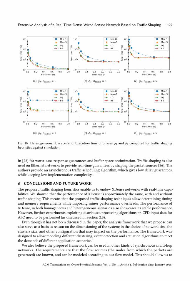
Extensive Analysis of a Real-Time Dense Wired Sensor Network Based on Traffic Shaping 1:25
0.0 0.2 0.4 0.6 0.8 1.0Burstiness ( )
101
102
103
104
Tota
l tim
e (T
TS)
Min-OMax-SLQBE
(a) ϕ3, nradius = 1
0.0 0.2 0.4 0.6 0.8 1.0Burstiness ( )
101
102
103
104
Tota
l tim
e (T
TS)
Min-OMax-SLQBE
(b) ϕ3, nradius = 3
0.0 0.2 0.4 0.6 0.8 1.0Burstiness ( )
101
102
103
104
Tota
l tim
e (T
TS)
Min-OMax-SLQBE
(c) ϕ3, nradius = 5
0.0 0.2 0.4 0.6 0.8 1.0Burstiness ( )
101
102
103
104
Tota
l tim
e (T
TS)
Min-OMax-SLQBE
(d) ϕ4, nradius = 1
0.0 0.2 0.4 0.6 0.8 1.0Burstiness ( )
101
102
103
104
Tota
l tim
e (T
TS)
Min-OMax-SLQBE
(e) ϕ4, nradius = 3
0.0 0.2 0.4 0.6 0.8 1.0Burstiness ( )
101
102
103
104
Tota
l tim
e (T
TS)
Min-OMax-SLQBE
(f) ϕ4, nradius = 5
Fig. 16. Heterogeneous flow scenario: Execution time of phases ϕ3 and ϕ4 computed for traffic shapingheuristics against simulation.
in [22] for worst-case response guarantees and buffer space optimization. Traffic shaping is alsoused on Ethernet networks to provide real-time guarantees by shaping the packet sources [36]. Theauthors provide an asynchronous traffic scheduling algorithm, which gives low delay guarantees,while keeping low implementation complexity.
6 CONCLUSIONS AND FUTURE WORK
The proposed traffic shaping heuristics enable us to endow XDense networks with real-time capa-bilities. We showed that the performance of XDense is approximately the same, with and withouttraffic shaping. This means that the proposed traffic shaping techniques allow determining timingand memory requirements while imposing minor performance overheads. The performance ofXDense, in both homogeneous and heterogeneous scenarios also showcases its stable performance.However, further experiments exploiting distributed processing algorithms on CFD input data forAFC need to be performed (as discussed in Section 2.3).
Even though it has not been discussed in the paper, the analysis framework that we propose canalso serve as a basis to reason on the dimensioning of the system; in the choice of network size, theclusters size, and other configuration that may impact on the performance. The framework wasdesigned to allow modeling different clustering, event detection and actuation algorithms, to meetthe demands of different application scenarios.We also believe the proposed framework can be used in other kinds of synchronous multi-hop
networks. The requirements are that the flow sources (the nodes from which the packets aregenerated) are known, and can be modeled according to our flow model. This should allow us to
ACM Transactions on Cyber-Physical Systems, Vol. 1, No. 1, Article 1. Publication date: January 2018.
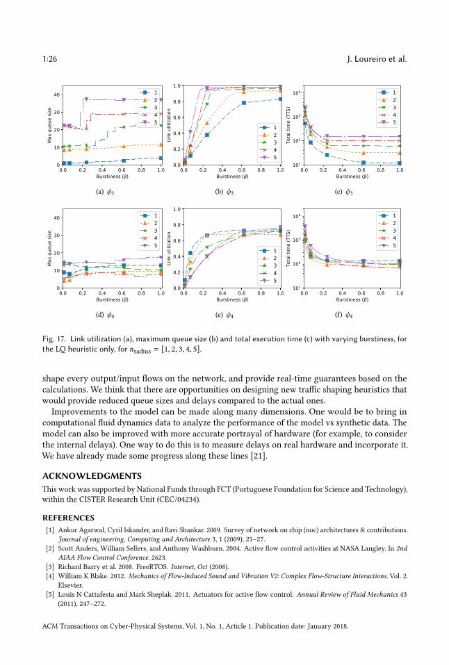
1:26 J. Loureiro et al.
0.0 0.2 0.4 0.6 0.8 1.0Burstiness ( )
0
10
20
30
40
Max
que
ue si
ze
12345
(a) ϕ3
0.0 0.2 0.4 0.6 0.8 1.0Burstiness ( )
0.0
0.2
0.4
0.6
0.8
1.0
Link
utiliz
atio
n
12345
(b) ϕ3
0.0 0.2 0.4 0.6 0.8 1.0Burstiness ( )
101
102
103
104
Tota
l tim
e (T
TS)
12345
(c) ϕ3
0.0 0.2 0.4 0.6 0.8 1.0Burstiness ( )
0
10
20
30
40
Max
que
ue si
ze
12345
(d) ϕ4
0.0 0.2 0.4 0.6 0.8 1.0Burstiness ( )
0.0
0.2
0.4
0.6
0.8
1.0
Link
utiliz
atio
n
12345
(e) ϕ4
0.0 0.2 0.4 0.6 0.8 1.0Burstiness ( )
101
102
103
104
Tota
l tim
e (T
TS)
12345
(f) ϕ4
Fig. 17. Link utilization (a), maximum queue size (b) and total execution time (c) with varying burstiness, forthe LQ heuristic only, for nradius = [1, 2, 3, 4, 5].
shape every output/input flows on the network, and provide real-time guarantees based on thecalculations. We think that there are opportunities on designing new traffic shaping heuristics thatwould provide reduced queue sizes and delays compared to the actual ones.
Improvements to the model can be made along many dimensions. One would be to bring incomputational fluid dynamics data to analyze the performance of the model vs synthetic data. Themodel can also be improved with more accurate portrayal of hardware (for example, to considerthe internal delays). One way to do this is to measure delays on real hardware and incorporate it.We have already made some progress along these lines [21].
ACKNOWLEDGMENTS
This work was supported by National Funds through FCT (Portuguese Foundation for Science and Technology),
within the CISTER Research Unit (CEC/04234).
REFERENCES
[1] Ankur Agarwal, Cyril Iskander, and Ravi Shankar. 2009. Survey of network on chip (noc) architectures & contributions.
Journal of engineering, Computing and Architecture 3, 1 (2009), 21ś27.
[2] Scott Anders, William Sellers, and Anthony Washburn. 2004. Active flow control activities at NASA Langley. In 2nd
AIAA Flow Control Conference. 2623.
[3] Richard Barry et al. 2008. FreeRTOS. Internet, Oct (2008).
[4] William K Blake. 2012. Mechanics of Flow-Induced Sound and Vibration V2: Complex Flow-Structure Interactions. Vol. 2.
Elsevier.
[5] Louis N Cattafesta and Mark Sheplak. 2011. Actuators for active flow control. Annual Review of Fluid Mechanics 43
(2011), 247ś272.
ACM Transactions on Cyber-Physical Systems, Vol. 1, No. 1, Article 1. Publication date: January 2018.

Extensive Analysis of a Real-Time Dense Wired Sensor Network Based on Traffic Shaping 1:27
[6] R. L. Cruz. 1991. A calculus for network delay. I. Network elements in isolation. IEEE Transactions on Information
Theory 37, 1 (Jan 1991), 114ś131. https://doi.org/10.1109/18.61109
[7] Artem Dementyev, Hsin-Liu (Cindy) Kao, and Joseph A. Paradiso. 2015. SensorTape: Modular and Programmable
3D-Aware Dense Sensor Network on a Tape. In Proceedings of the 28th Annual ACM Symposium on User Interface
Software & Technology (UIST ’15). ACM, New York, NY, USA, 649ś658. https://doi.org/10.1145/2807442.2807507
[8] Rostislav Reuven Dobkin, Arkadiy Morgenshtein, Avinoam Kolodny, and Ran Ginosar. 2008. Parallel vs. Serial On-chip
Communication. In Proceedings of the 2008 International Workshop on System Level Interconnect Prediction (SLIP ’08).
ACM, New York, NY, USA, 43ś50. https://doi.org/10.1145/1353610.1353620
[9] Xing Fan, Magnus Jonsson, and Jan Jonsson. 2009. Guaranteed real-time communication in packet-switched networks
with FCFS queuing. Computer Networks 53, 3 (2009), 400 ś 417. https://doi.org/10.1016/j.comnet.2008.10.018
[10] M. Fidler. 2010. Survey of deterministic and stochastic service curve models in the network calculus. IEEE Communica-
tions Surveys Tutorials 12, 1 (First 2010), 59ś86. https://doi.org/10.1109/SURV.2010.020110.00019
[11] Jingcao Hu and Radu Marculescu. 2003. Energy-aware Mapping for Tile-based NoC Architectures Under Performance
Constraints. In Proceedings of the 2003 Asia and South Pacific Design Automation Conference (ASP-DAC ’03). ACM, New
York, NY, USA, 233ś239. https://doi.org/10.1145/1119772.1119818
[12] Leandro Soares Indrusiak. 2014. End-to-end schedulability tests for multiprocessor embedded systems based on
networks-on-chip with priority-preemptive arbitration. Journal of Systems Architecture 60, 7 (2014), 553 ś 561.
https://doi.org/10.1016/j.sysarc.2014.05.002
[13] Nobuhide Kasagi, Yuji Suzuki, and Koji Fukagata. 2009. Microelectromechanical systems-based feedback control of
turbulence for skin friction reduction. Annual review of fluid mechanics 41 (2009), 231ś251.
[14] N. K. Kavaldjiev and G. J. M. Smit. 2003. A Survey of Efficient On-Chip Communications for SoC.
http://eprints.eemcs.utwente.nl/833/. In 4th PROGRESS Symposium on Embedded Systems, Nieuwegein, The Netherlands.
Technology Foundation STW, Utrecht, The Netherlands, 129ś140.
[15] Fotis Kopsaftopoulos, Raphael Nardari, Yu-Hung Li, and FK Chang. 2015. Experimental identification of structural
dynamics and aeroelastic properties of a self-sensing smart composite wing. In Proceedings of the 10th International
Workshop on Structural Health Monitoring, Stanford, CA.
[16] Shashi Kumar, Axel Jantsch, J-P Soininen, Martti Forsell, Mikael Millberg, Johny Oberg, Kari Tiensyrja, and Ahmed
Hemani. 2002. A network on chip architecture and design methodology. In VLSI, 2002. Proceedings. IEEE Computer
Society Annual Symposium on. IEEE, 105ś112.
[17] Joshua Lifton, Michael Broxton, and Joseph A. Paradiso. 2005. Experiences and Directions in Pushpin Computing. In
Proceedings of the 4th International Symposium on Information Processing in Sensor Networks (IPSN ’05). IEEE Press,
Piscataway, NJ, USA, Article 57. http://dl.acm.org/citation.cfm?id=1147685.1147753
[18] J. Loureiro, R. Rangarajan, B. Nikolic, L. Indrusiak, and E. Tovar. 2017. Real-time dense wired sensor network based
on traffic shaping. In 2017 IEEE 23rd International Conference on Embedded and Real-Time Computing Systems and
Applications (RTCSA). 1ś10. https://doi.org/10.1109/RTCSA.2017.8046307
[19] João Loureiro, Raghuraman Rangarajan, and Eduardo Tovar. [n. d.]. Demo Abstract: Towards the Development of
XDense, A Sensor Network for Dense Sensing. 12th European Conference on Wireless Sensor Networks (EWSN) ([n. d.]),
23. www.cister.isep.ipp.pt/ewsn2015/EWSN15PosterDemoProc_WEB.pdf#page=24
[20] J. Loureiro, R. Rangarajan, and E. Tovar. 2015. Distributed Sensing of Fluid Dynamic Phenomena with the XDense
Sensor Grid Network. In Cyber-Physical Systems, Networks, and Applications (CPSNA), 2015 IEEE 3rd International
Conference on. 54ś59. https://doi.org/10.1109/CPSNA.2015.19
[21] João Loureiro, Pedro Santos, Raghuraman Rangarajan, and Eduardo Tovar. 2017. Simulation Module and Tools for
XDense Sensor Network. In Proceedings of the Workshop on Ns-3 (WNS3 ’17). ACM, New York, NY, USA, 110ś117.
https://doi.org/10.1145/3067665.3067680
[22] Sorin Manolache, Petru Eles, and Zebo Peng. 2006. Buffer Space Optimisation with Communication Synthesis and
Traffic Shaping for NoCs. In Proceedings of the Conference on Design, Automation and Test in Europe: Proceedings (DATE
’06). European Design and Automation Association, 3001 Leuven, Belgium, Belgium, 718ś723. http://dl.acm.org/
citation.cfm?id=1131481.1131683
[23] Behram F.T. Mistree and Joseph A. Paradiso. 2010. ChainMail: A Configurable Multimodal Lining to Enable Sensate
Surfaces and Interactive Objects. In Proceedings of the Fourth International Conference on Tangible, Embedded, and
Embodied Interaction (TEI ’10). ACM, New York, NY, USA, 65ś72. https://doi.org/10.1145/1709886.1709899
[24] F. Palacios, J. Alonso, K. Duraisamy, M. Colonno, J. Hicken, A. Aranake, A. Campos, S. Copeland, T. Economon, A.
Lonkar, et al. 2013. Stanford University Unstructured (SU 2): An Open-Source Integrated Computational Environment
for Multi-Physics Simulation and Design. In 51st AIAA Aerospace Sciences Meeting Including the New Horizons Forum
and Aerospace Exposition. 287.
[25] Alexandros Pantelopoulos and Nikolaos G Bourbakis. 2010. A survey on wearable sensor-based systems for health
monitoring and prognosis. IEEE Transactions on Systems, Man, and Cybernetics, Part C (Applications and Reviews) 40, 1
ACM Transactions on Cyber-Physical Systems, Vol. 1, No. 1, Article 1. Publication date: January 2018.

1:28 J. Loureiro et al.
(2010), 1ś12.
[26] Ruiyi Que and Rong Zhu. 2012. Aircraft Aerodynamic Parameter Detection Using Micro Hot-Film Flow Sensor Array
and BP Neural Network Identification. Sensors 12, 8 (2012), 10920ś10929. https://doi.org/10.3390/s120810920
[27] D. Rahmati, S. Murali, L. Benini, F. Angiolini, G. De Micheli, and H. Sarbazi-Azad. 2013. Computing Accurate
Performance Bounds for Best Effort Networks-on-Chip. IEEE Trans. Comput. 62, 3 (March 2013), 452ś467. https:
//doi.org/10.1109/TC.2011.240
[28] J Reneaux et al. 2004. Overview on drag reduction technologies for civil transport aircraft. ONERA: Tire a Part 153
(2004), 1ś18.
[29] Stephen K Robinson. 1991. Coherent motions in the turbulent boundary layer. Annual Review of Fluid Mechanics 23, 1
(1991), 601ś639.
[30] Carlos Rodrigues, Carlos FÃľlix, Armindo Lage, and Joaquim Figueiras. 2010. Development of a long-term monitoringsystem based on FBG sensors applied to concrete bridges. Engineering Structures 32, 8 (2010), 1993 ś 2002. https://doi.org/10.1016/j.engstruct.2010.02.033
[31] Artur Saudabayev and Huseyin Atakan Varol. 2015. Sensors for robotic hands: A survey of state of the art. IEEE Access
3 (2015), 1765ś1782.[32] V Schmitt and F Charpin. 1979. Pressure distributions on the ONERA-M6-Wing at transonic Mach numbers. Experi-
mental data base for computer program assessment 4 (1979).[33] JH Seo, F Cadieux, R Mittal, E Deem, and L Cattafesta. 2018. Effect of synthetic jet modulation schemes on the reduction
of a laminar separation bubble. Physical Review Fluids 3, 3 (2018), 033901.[34] Zheng Shi and Alan Burns. 2008. Real-Time Communication Analysis for On-Chip Networks withWormhole Switching.
In Proceedings of the Second ACM/IEEE International Symposium on Networks-on-Chip (NOCS ’08). IEEE ComputerSociety, Washington, DC, USA, 161ś170. http://dl.acm.org/citation.cfm?id=1397757.1397996
[35] Vijay Sivaraman, Fabio M. Chiussi, and Mario Gerla. 2006. Deterministic end-to-end delay guarantees with ratecontrolled {EDF} scheduling. Performance Evaluation 63, 4âĂŞ5 (2006), 509 ś 519. https://doi.org/10.1016/j.peva.2005.04.002
[36] J. Specht and S. Samii. 2016. Urgency-Based Scheduler for Time-Sensitive Switched Ethernet Networks. In 2016 28th
Euromicro Conference on Real-Time Systems (ECRTS). 75ś85. https://doi.org/10.1109/ECRTS.2016.27[37] Lau Troy M, Gwin Joseph T, and Ferris Daniel P. 2012. How many electrodes are really needed for EEG-based mobile
brain imaging? Journal of Behavioral and Brain Science 2012 (2012).[38] Tony Washburn. 2010. Airframe Drag/Weight Reduction Technologies. Green Aviation Summit-Fuel Burn Reduction,
NASA Ames Research Centre (2010).[39] M Watson, AJ Jaworski, and NJ Wood. 2007. Application of synthetic jet actuators for the modification of the
characteristics of separated shear layers on slender wings. The Aeronautical Journal 111, 1122 (2007), 519ś529.
ACM Transactions on Cyber-Physical Systems, Vol. 1, No. 1, Article 1. Publication date: January 2018.