Extensions of the Kac N-particle Extensions of the Kac N-particle model to model to

multi-linear interactionsmulti-linear interactions

Irene M. GambaDepartment of Mathematics and ICES

The University of Texas at Austin

Classical and Random Dynamics in Mathematical Physics CoLab UT Austin-Portugal, April 2010

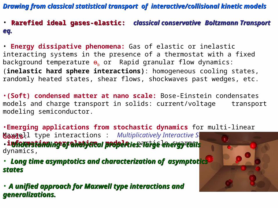
Drawing from classical statistical transport of interactive/collisional kinetic modelsDrawing from classical statistical transport of interactive/collisional kinetic models

• Rarefied ideal gases-elastic:Rarefied ideal gases-elastic: classical conservativeclassical conservative Boltzmann Transport eq.Boltzmann Transport eq.

• Energy dissipative phenomena: Gas of elastic or inelastic interacting systems in the presence of a thermostat with a fixed background temperature өb or Rapid granular flow dynamics: (inelastic hard sphere interactions): homogeneous cooling states, randomly heated states, shear flows, shockwaves past wedges, etc.

•(Soft) condensed matter at nano scale: Bose-Einstein condensates models and charge transport in solids: current/voltage transport modeling semiconductor.

•Emerging applications from stochastic dynamics for multi-linear Maxwell type interactions : Multiplicatively Interactive Stochastic Processes: information percolation modelsinformation percolation models, particle swarms in population dynamics,

Goals: • Understanding of analytical properties: large energy tailsUnderstanding of analytical properties: large energy tails • Long time asymptotics and characterization of asymptotics statesLong time asymptotics and characterization of asymptotics states

• A unified approach for Maxwell type interactions and A unified approach for Maxwell type interactions and generalizations.generalizations.

•Spectral-Lagrangian solvers for dissipative interactionsSpectral-Lagrangian solvers for dissipative interactions

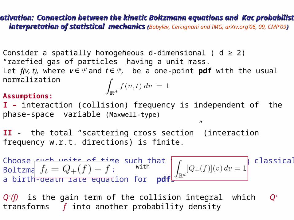
Consider a spatially homogeneous d-dimensional ( d ≥ 2) “rarefied gas of particles” having a unit mass. Let f(v, t), where v ∈ d and t ∈ +, be a one-point pdf with the usual normalization

Assumptions: I – interaction (collision) frequency is independent of the phase-space variable (Maxwell-type)

II - the total “scattering cross section” (interaction frequency w.r.t. directions) is finite.

Choose such units of time such that the corresponding classical Boltzmann eqs. reads asa birth-death rate equation for pdfs

with

Q+(f) is the gain term of the collision integral which Q+ transforms f into another probability density

Motivation:Motivation: Connection between the kinetic Boltzmann equations and Kac probabilistic Connection between the kinetic Boltzmann equations and Kac probabilistic interpretation of statistical mechanics interpretation of statistical mechanics ((Bobylev, Cercignani and IMG, arXiv.org’06, 09, CMP’09))

The same stochastic model admits other possible generalizationsThe same stochastic model admits other possible generalizations. For example we can also include multiple interactions and interactions with a background (thermostat).This type of model will formally correspond to a version of the kinetic equation for some Q+(f).

where Q(j)+ , j = 1, . . . ,M, are j-linear positive operators describing interactions of j ≥ 1 particles,

and αj ≥ 0 are relative probabilities of such interactions, where

Assumption: Temporal evolution of the system is invariant under scaling transformations in phase space: if St is the evolution operator for the given N-particle system such that

St{v1(0), . . . , vM(0)} = {v1(t), . . . , vM(t)} , t ≥ 0 ,

then St{λv1(0), . . . , λ vM(0)} = {λv1(t), . . . , λvM(t)} for any constant λ > 0

which leads to the property Q+

(j) (Aλ f) = Aλ Q+(j) (f), Aλ f(v) = λd f(λ v) , λ > 0, (j = 1, 2, .,M)

Note that the transformation Aλ is consistent with the normalization of f with respect to v.

Note: this property on Q(j)+ is needed to make the consistent with the classical BTE for Maxwell-type interactions

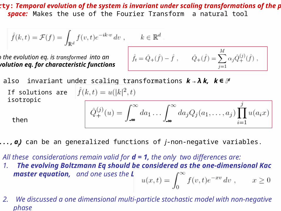
Property: Temporal evolution of the system is invariant under scaling transformations of the phase space: Makes the use of the Fourier Transform a natural tool

so the evolution eq. is transformed into an evolution eq. for characteristic functions

which is also invariant under scaling transformations k → λ k, k ∈ d

All these considerations remain valid for d = 1, the only two differences are:1. The evolving Boltzmann Eq should be considered as the one-dimensional Kac master

equation, and one uses the Laplace transform

2. We discussed a one dimensional multi-particle stochastic model with non-negative phase variables v in R+,

If solutions are isotropic

then

where Qj(a1, . . . , aj) can be an generalized functions of j-non-negative variables.

-∞-∞

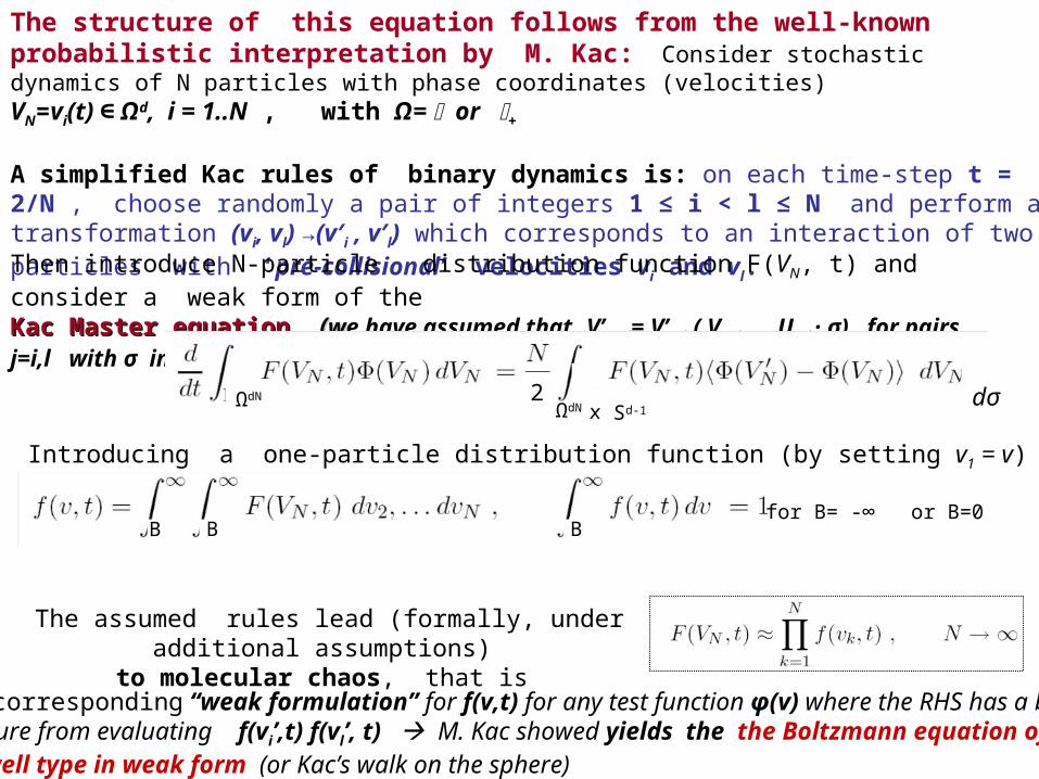
The structure of this equation follows from the well-known probabilistic interpretation by M. Kac: Consider stochastic dynamics of N particles with phase coordinates (velocities) VN=vi(t) ∈ Ωd, i = 1..N , with Ω= or +

A simplified Kac rules of binary dynamics is: on each time-step t = 2/N , choose randomly a pair of integers 1 ≤ i < l ≤ N and perform a transformation (vi, vl) →(v′i , v′l) which corresponds to an interaction of two particles with ‘pre-collisional’ velocities vi and vl.

Then introduce N-particle distribution function F(VN, t) and consider a weak form of the

Kac Master equation Kac Master equation ((wwe have assumed that V’ N j= V’N j ( VN j , UN j · σ) for pairs j=i,l with σ in a compact set)

The assumed rules lead (formally, under additional assumptions) to molecular chaos, that is

Introducing a one-particle distribution function (by setting v1 = v) and the hierarchy reduction

The corresponding “weak formulation” for f(v,t) for any test function φ(v) where the RHS has a bilinear structure from evaluating f(vi’,t) f(vl’, t) M. Kac showed yields the the Boltzmann equation of Maxwell type in weak form (or Kac’s walk on the sphere)

2ΩdN

ΩdN x Sd-1

B BBfor B= -∞ or B=0

dσ

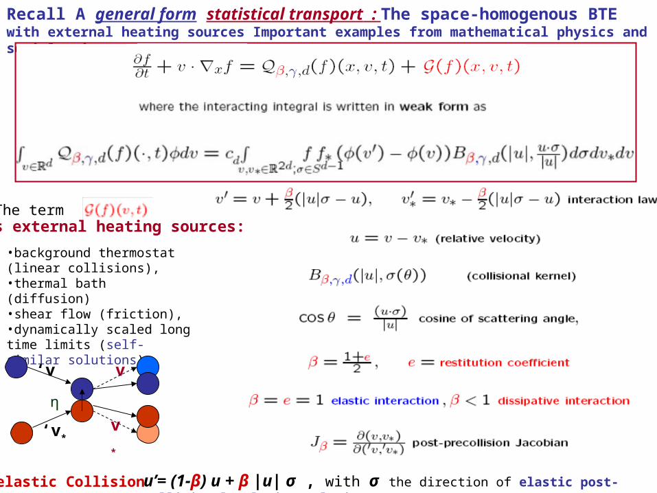
Recall A general form statistical transport : The space-homogenous BTE with external heating sources Important examples from mathematical physics and social sciences:

The termmodels external heating sources:

•background thermostat (linear collisions), •thermal bath (diffusion)•shear flow (friction), •dynamically scaled long time limits (self-similar solutions).

Inelastic Collision u’= (1-β) u + β |u| σ , with σ the direction of elastic post-collisional relative velocity

‘v

‘v*

v

v*

η

Qualitative issues on elastic: Bobylev,78-84, and inelastic: Bobylev, Carrillo I.G, JSP2000, Bobylev, Cercignani 03-04,with Toscani 03, with I.M.G. JSP’06, arXiv.org’06, CMP’09

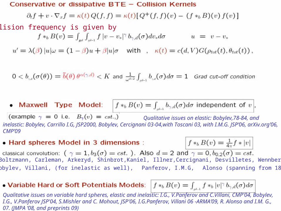
Classical work of Boltzmann, Carleman, Arkeryd, Shinbrot,Kaniel, Illner,Cercignani, Desvilletes, Wennberg,

Di-Perna, Lions, Bobylev, Villani, (for inelastic as well), Panferov, I.M.G, Alonso (spanning from 1888 to 2009)

Qualitative issues on variable hard spheres, elastic and inelastic: I.G., V.Panferov and C.Villani, CMP'04, Bobylev, I.G., V.Panferov JSP'04, S.Mishler and C. Mohout, JSP'06, I.G.Panferov, Villani 06 -ARMA’09, R. Alonso and I.M. G., 07. (JMPA ‘08, and preprints 09)

The collision frequency is given by

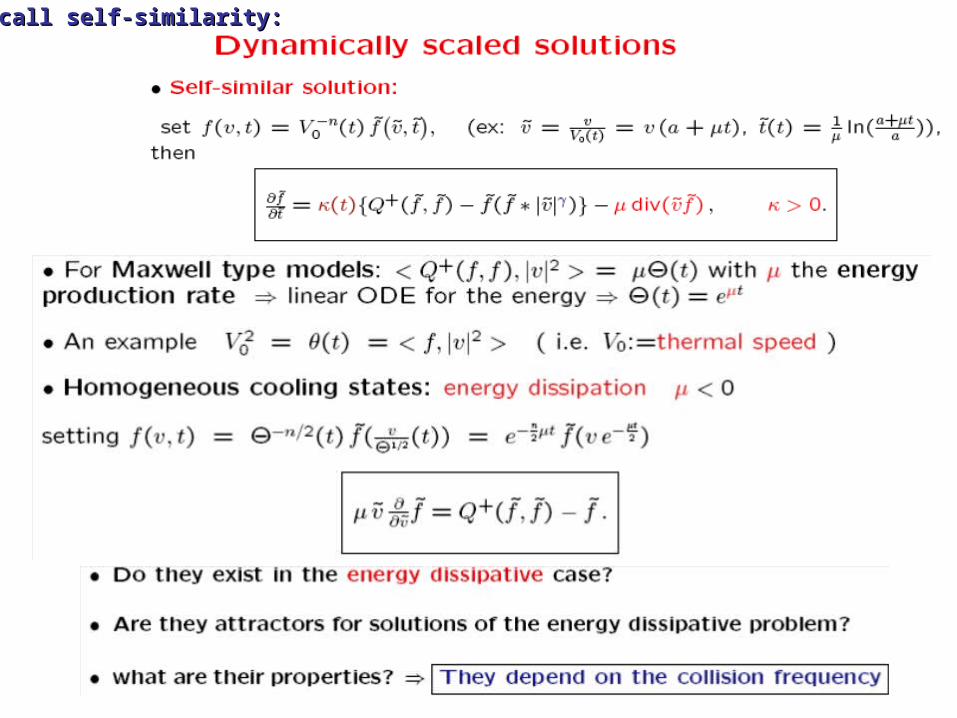
Recall self-similarity:Recall self-similarity:

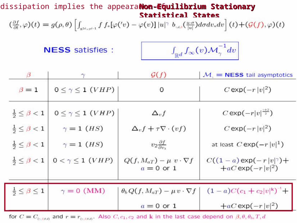
Non-Equilibrium Stationary Statistical StatesNon-Equilibrium Stationary Statistical StatesEnergy dissipation implies the appearance of

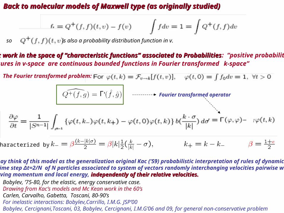
Back to molecular models of Maxwell type (as originally studied)Back to molecular models of Maxwell type (as originally studied)

Bobylev, ’75-80, for the elastic, energy conservative case.Drawing from Kac’s models and Mc Kean work in the 60’sCarlen, Carvalho, Gabetta, Toscani, 80-90’s For inelastic interactions: Bobylev,Carrillo, I.M.G. JSP’00Bobylev, Cercignani,Toscani, 03, Bobylev, Cercignani, I.M.G’06 and 09, for general non-conservative problem

characterized by

so is also a probability distribution function in v.

The Fourier transformed problem:

One may think of this model as the generalization original Kac (’59) probabilistic interpretation of rules of dynamics on each time step Δt=2/N of N particles associated to system of vectors randomly interchanging velocities pairwise while preserving momentum and local energy, independently of their relative velocities.independently of their relative velocities.

Then: work in the space of “characteristic functions” associated to ProbabilitiesThen: work in the space of “characteristic functions” associated to Probabilities: “positive probability measures in v-space are continuous bounded functions in Fourier transformed k-space”

Fourier transformed operatorΓ

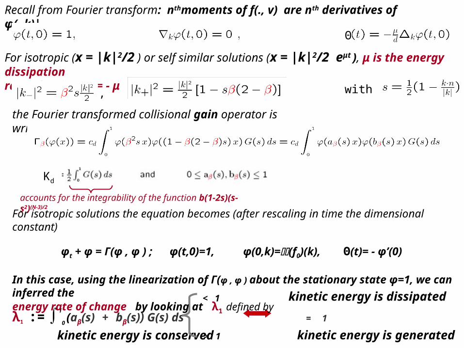
accounts for the integrability of the function b(1-2s)(s-s2)(N-3)/2

λ1 := ∫1

0 (aβ(s) + bβ(s)) G(s) ds = 1 kinetic energy is conserved

< 1 kinetic energy is dissipated

> 1 kinetic energy is generated

For isotropic solutions the equation becomes (after rescaling in time the dimensional constant)

φt + φ = Γ(φ , φ ) ; φ(t,0)=1, φ(0,k)=(f0)(k), Θ(t)= - φ’(0)

In this case, using the linearization of Γ(φ , φ ) about the stationary state φ=1, we can inferred the energy rate of change by looking at λ1 defined by

For isotropic (x = |k|2/2 ) or self similar solutions (x = |k|2/2 eμt ), μ is the energy dissipationrate, that is: Θt = - μ Θ , and

Recall from Fourier transform: nthmoments of f(., v) are nth derivatives of φ(.,k)|k=0

Θ

the Fourier transformed collisional gain operator is written

, with

Kd

Existence, asymptotic behavior - self-similar solutions and power like tails: From a unified point of energy dissipative Maxwell type models: λ1 energy dissipation rate (Bobylev, I.M.G.JSP’06, Bobylev,Cercignani,I.G. arXiv.org’06- CMP’09)

ExamplesExamples

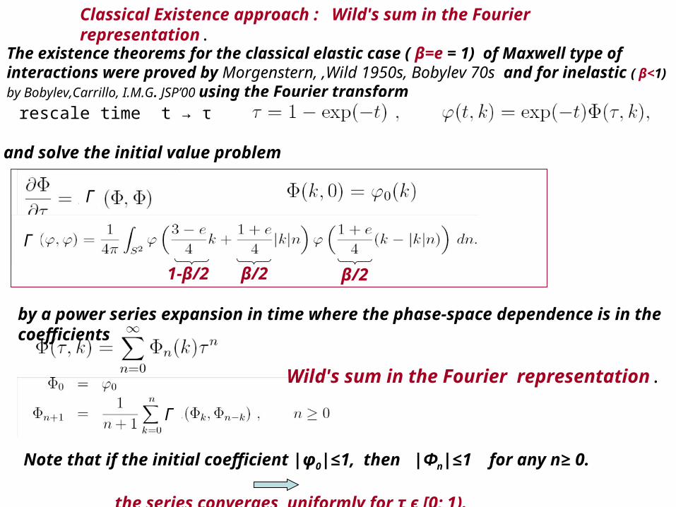
The existence theorems for the classical elastic case ( β=e = 1) of Maxwell type of interactions were proved by Morgenstern, ,Wild 1950s, Bobylev 70s and for inelastic ( β<1) by Bobylev,Carrillo, I.M.G.

JSP’00 using the Fourier transform

Note that if the initial coefficient |φ0|≤1, then |Фn|≤1 for any n≥ 0. the series converges uniformly for τ ϵ [0; 1).

Classical Existence approach : Wild's sum in the Fourier representation.

Γ

Γ

Γ

• rescale time t → τ

and solve the initial value problem

by a power series expansion in time where the phase-space dependence is in the coefficients

Wild's sum in the Fourier representation.

β/2β/21-β/2

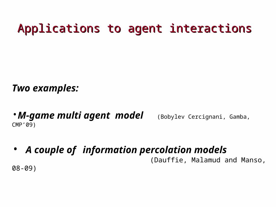
Applications to agent interactionsApplications to agent interactions

Two examples:

•M-game multi agent model (Bobylev Cercignani, Gamba, CMP’09)

• A couple of information percolation models (Dauffie, Malamud and Manso, 08-09)

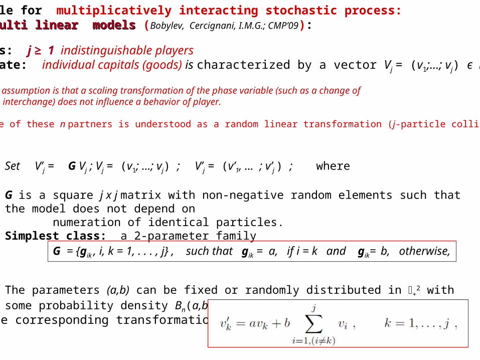
An example for multiplicatively interacting stochastic process:M-game multi linear modelsM-game multi linear models (Bobylev, Cercignani, I.M.G.; CMP’09):

particles: j ≥ 1 indistinguishable players phase state: individual capitals (goods) is characterized by a vector Vj = (v1;…; vj) ϵ j

+

• A realistic assumption is that a scaling transformation of the phase variable (such as a change of goods interchange) does not influence a behavior of player.

• The game of these n partners is understood as a random linear transformation (j-particle collision)

The parameters (a,b) can be fixed or randomly distributed in +2 with some probability density Bn(a,b).

The corresponding transformation is

Set V’j = G Vj ; Vj = (v1; …; vj) ; V’j = (v’1, … ; v’j ) ; where

G is a square j x j matrix with non-negative random elements such that the model does not depend on numeration of identical particles.Simplest class: a 2-parameter family

G = {gik , i, k = 1, . . . , j} , such that gik = a, if i = k and gik= b, otherwise,

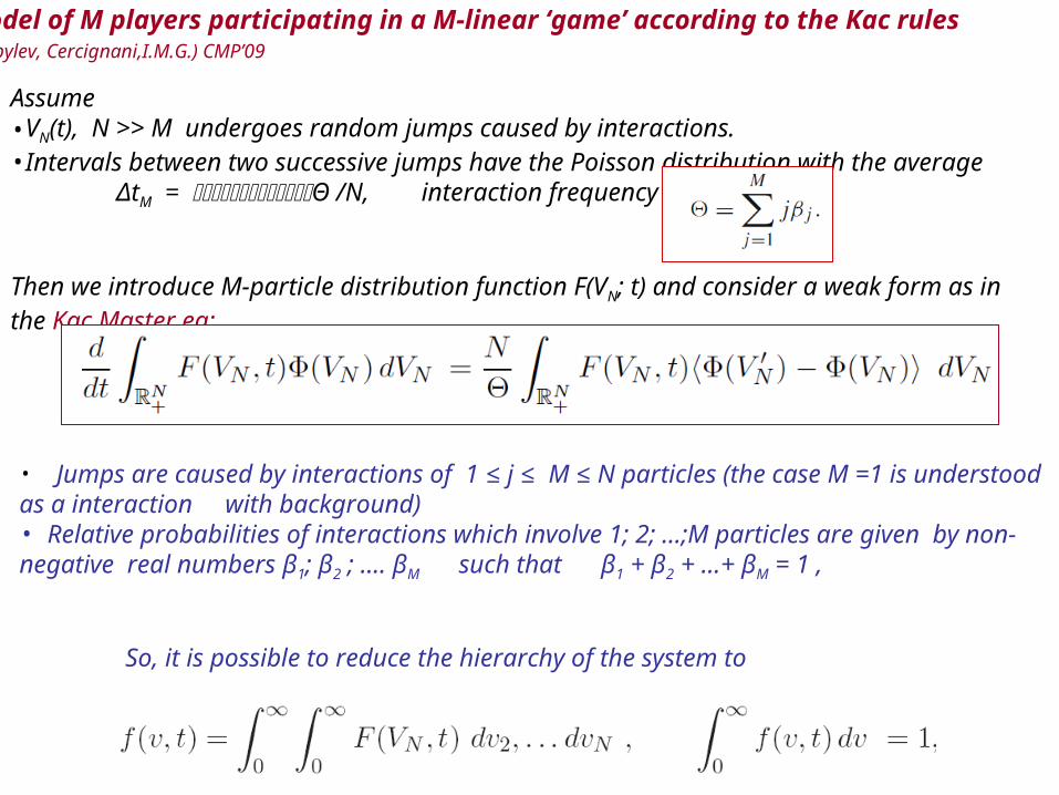
• Jumps are caused by interactions of 1 ≤ j ≤ M ≤ N particles (the case M =1 is understood as a interaction with background) • Relative probabilities of interactions which involve 1; 2; …;M particles are given by non-negative real numbers β1; β2 ; …. βM such that β1 + β2 + …+ βM = 1 ,

Assume •VN(t), N >> M undergoes random jumps caused by interactions.•Intervals between two successive jumps have the Poisson distribution with the average

ΔtM = Θ /N, interaction frequency with

Then we introduce M-particle distribution function F(VN; t) and consider a weak form as in the Kac Master eq:

Model of M players participating in a M-linear ‘game’ according to the Kac rules (Bobylev, Cercignani,I.M.G.) CMP’09

So, it is possible to reduce the hierarchy of the system to

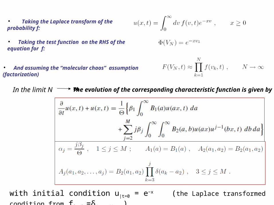
In the limit N ∞

• Taking the test function on the RHS of the equation for f:

• Taking the Laplace transform of the probability f:

• And assuming the “molecular chaos” assumption (factorization)

The evolution of the corresponding characteristic function is given by

with initial condition u|t=0 = e−x (the Laplace transformed condition from f|t=0 =δ(v − 1) )

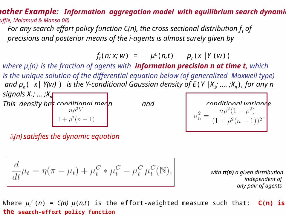
For any search-effort policy function C(n), the cross-sectional distribution f t of precisions and posterior means of the i-agents is almost surely given by ft(n; x; w) = μC(n,t) pn(x |Y (w))

Another Example: Information aggregation model with equilibrium search dynamics (Duffie, Malamud & Manso 08)

where μt(n) is the fraction of agents with information precision n at time t, which is the unique solution of the differential equation below (of generalized Maxwell type) and pn( x| Y(w) ) is the Y-conditional Gaussian density of E(Y |X1; …. ;Xn), for any n signals X1; … ;Xn. This density has conditional mean and conditional variance

t(n) satisfies the dynamic equation

with π(n) a given distribution independent of any pair of agents

Where μtC (n) = C(n) μ(n,t) is the effort-weighted measure such that: C(n) is the search-effort policy function

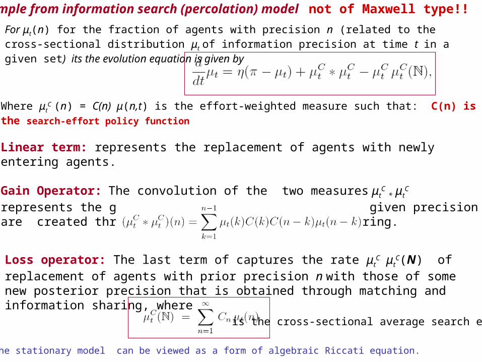
For μt(n) for the fraction of agents with precision n (related to the cross-sectional distribution μt of information precision at time t in a given set) its the evolution equation is given by

Where μtC (n) = C(n) μ(n,t) is the effort-weighted measure such that: C(n) is the search-effort policy function

Linear term: represents the replacement of agents with newly entering agents.

Gain Operator: The convolution of the two measures μtC * μt

C represents the gross rate at which new agents of a given precision are created through matching and information sharing.

Example from information search (percolation) model not of Maxwell type!!

Loss operator: The last term of captures the rate μtC μt

C(N) of replacement of agents with prior precision n with those of some new posterior precision that is obtained through matching and information sharing, where

is the cross-sectional average search effort

Remark: The stationary model can be viewed as a form of algebraic Riccati equation.

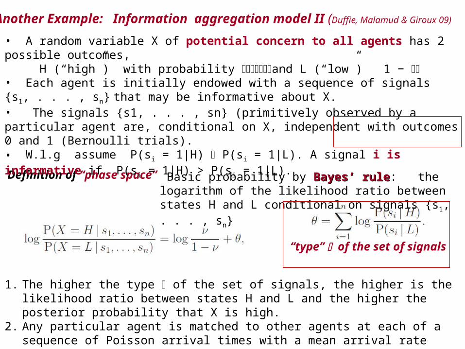
Another Example: Information aggregation model II (Duffie, Malamud & Giroux 09)

1. The higher the type of the set of signals, the higher is the likelihood ratio between states H and L and the higher the posterior probability that X is high.

2. Any particular agent is matched to other agents at each of a sequence of Poisson arrival times with a mean arrival rate (intensity) , which is the same across agents.

3. At each meeting time, m−1 other agents are randomly selected from the population of agents

Definition of “phase space” Basic probability by Bayes’ ruleBayes’ rule: the logarithm of the likelihood ratio between states H and L conditional on signals {s1, . . . , sn}

“type” of the set of signals

• A random variable X of potential concern to all agents has 2 possible outcomes, H (“high”) with probability and L (“low”) 1 − • Each agent is initially endowed with a sequence of signals {s1, . . . , sn} that may be informative about X. • The signals {s1, . . . , sn} (primitively observed by a particular agent are, conditional on X, independent with outcomes 0 and 1 (Bernoulli trials). • W.l.g assume P(si = 1|H) P(si = 1|L). A signal i is informative if P(si = 1|H) > P(si = 1|L).

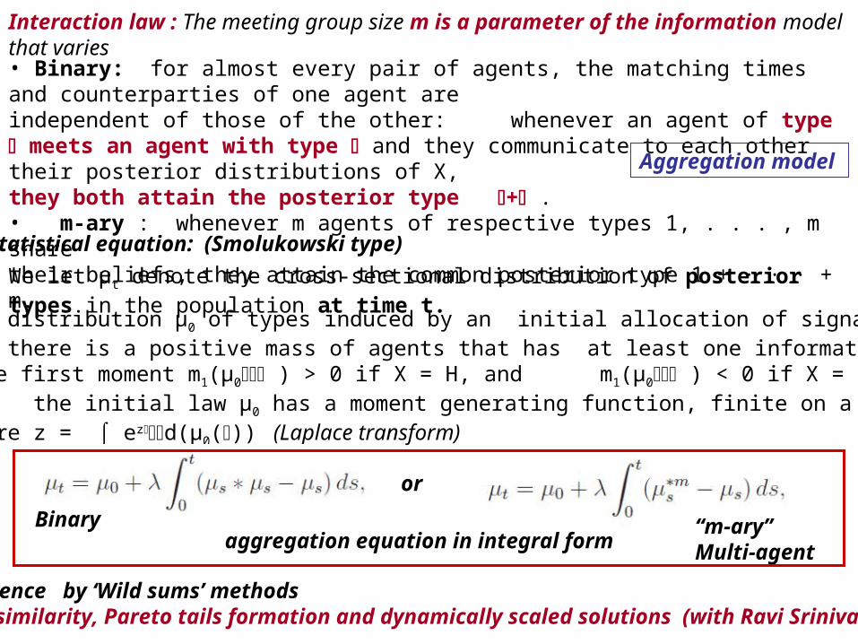
• Binary: for almost every pair of agents, the matching times and counterparties of one agent areindependent of those of the other: whenever an agent of type meets an agent with type and they communicate to each other their posterior distributions of X, they both attain the posterior type + .• m-ary : whenever m agents of respective types 1, . . . , m sharetheir beliefs, they attain the common posterior type 1 + · · · + m.

Interaction law : The meeting group size m is a parameter of the information model that varies

Aggregation model

We let μt denote the cross-sectional distribution of posterior types in the population at time t.

• The initial distribution μ0 of types induced by an initial allocation of signals to agents. • Assume that there is a positive mass of agents that has at least one informative signal. • That is, the first moment m1(μ0 ) > 0 if X = H, and m1(μ0 ) < 0 if X = L. • Assume that the initial law μ0 has a moment generating function, finite on a neighborhood of z = 0 , where z = ⌠ ezd(μ0()) (Laplace transform)

aggregation equation in integral formBinary

or

“m-ary”Multi-agent

Existence by ‘Wild sums’ methodsSelf-similarity, Pareto tails formation and dynamically scaled solutions (with Ravi Srinivasan)

Statistical equation: (Smolukowski type)

with V’m = G Vm ; Vm = (v1; …; vm) ; V’m = (v’1, … ; v’m) ; where

G is a square m x m matrix with entriesG = {gik = 1 , for all i, k = 1, . . . , m} ,

We notice the similarity with the the Kac model: let the type signals Vm and its posterior V’m

Then the m-particle distribution function F(VN, t) and the weak form of the

Kac Master equationKac Master equation

The assumed rules lead (formally, under additional assumptions) to molecular chaos, that is

Introducing a one-particle distribution function (by setting v1 = v) and the hierarchy reduction

2for N=m

Then the aggregation models hold for f(vm , t ) for either binary or multi-agent forms

The approach extends to more general information percolation models where the signal typedo not necessarily aggregate but “distributes ” itself between the posterior types (in collaboration with Ravi Srinivasan)

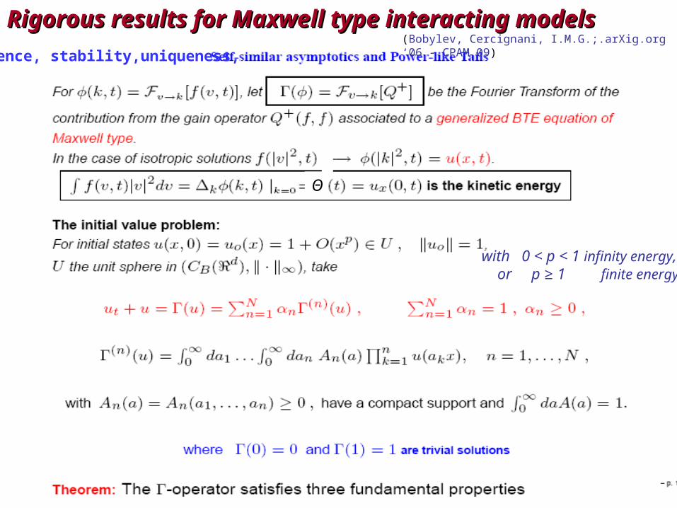
Existence, stability,uniqueness, (Bobylev, Cercignani, I.M.G.;.arXig.org ‘06 - CPAM 09)

with 0 < p < 1 infinity energy, or p ≥ 1 finite energy

Θ

Rigorous results for Maxwell type interacting modelsRigorous results for Maxwell type interacting models

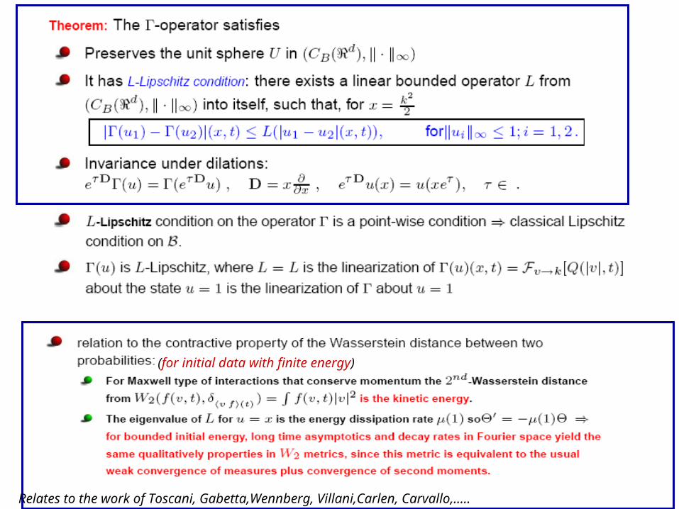
Relates to the work of Toscani, Gabetta,Wennberg, Villani,Carlen, Carvallo,…..

(for initial data with finite energy)

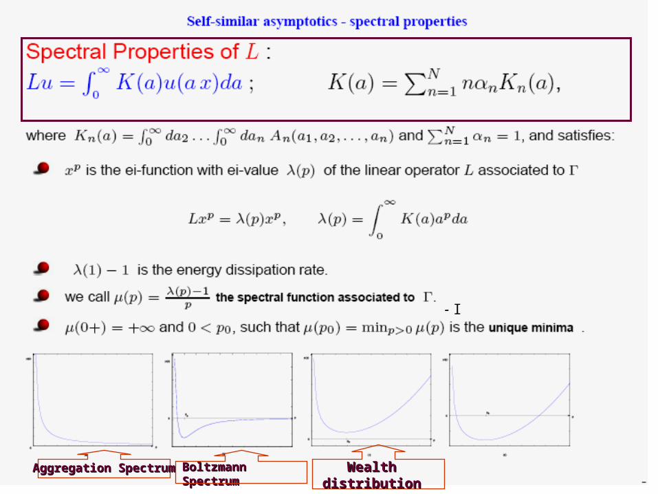
Boltzmann SpectrumBoltzmann Spectrum

- I

Aggregation SpectrumAggregation Spectrum Wealth Wealth distributiondistributionSpectrumSpectrum

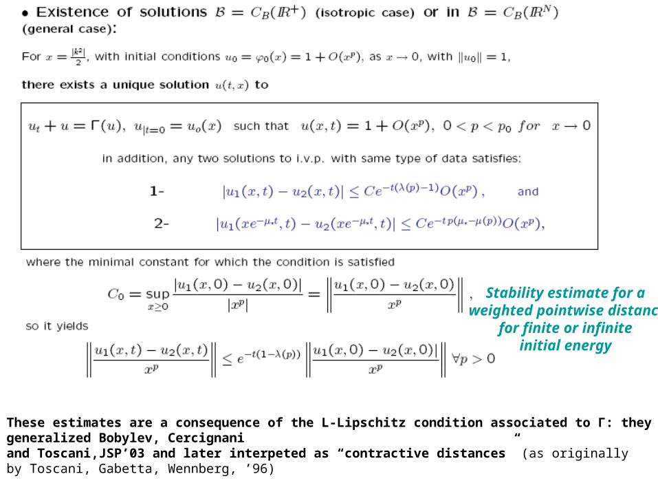
Stability estimate for a weighted pointwise distance

for finite or infinite initial energy

These estimates are a consequence of the L-Lipschitz condition associated to Γ: they generalized Bobylev, Cercignani and Toscani,JSP’03 and later interpeted as “contractive distances” (as originally by Toscani, Gabetta, Wennberg, ’96)

These estimates imply, jointly with the property of the invariance under dilations for Γ, selfsimilar asymptotics and the existence of non-trivial dynamically stable laws.

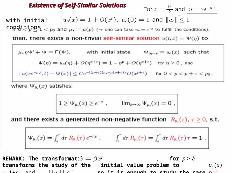
Existence of Self-Similar SolutionsExistence of Self-Similar Solutions

with initial conditions

REMARK: The transformation , for p > 0 transforms the study of the initial value problem to uo(x) = 1+x and ||uo|| ≤ 1 so it is enough to study the case p=1

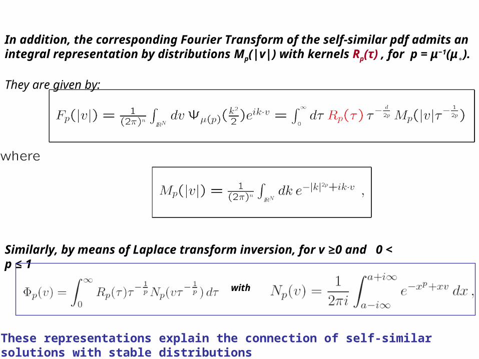
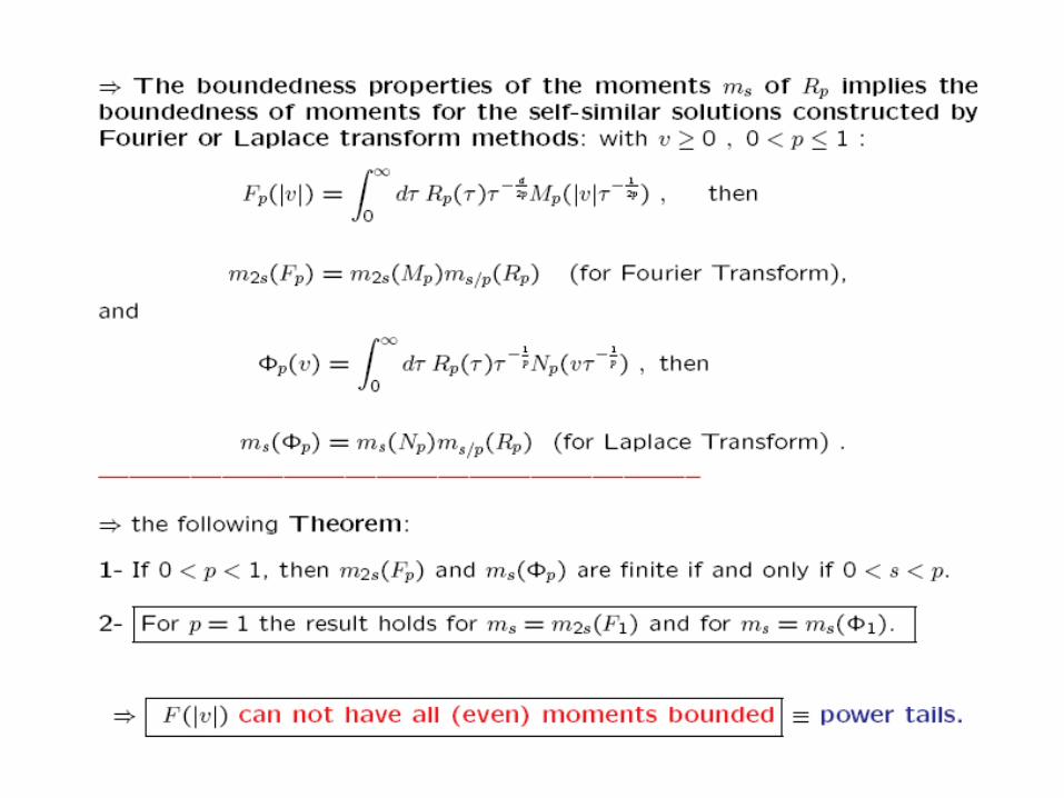
These representations explain the connection of self-similar solutions with stable distributions

Similarly, by means of Laplace transform inversion, for v ≥0 and 0 < p ≤ 1

with

In addition, the corresponding Fourier Transform of the self-similar pdf admits an integral representation by distributions Mp(|v|) with kernels Rp(τ) , for p = μ−1(μ∗).

They are given by:

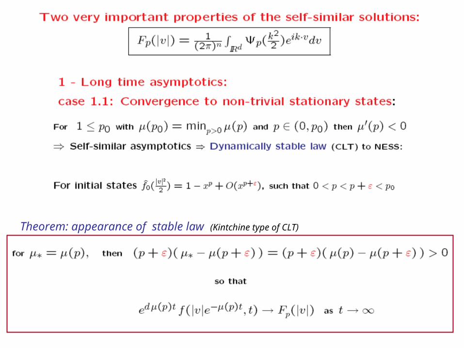
Theorem: appearance of stable law (Kintchine type of CLT)

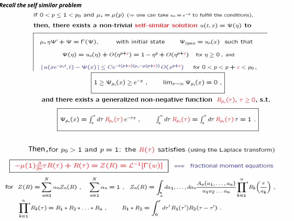
Recall the self similar problem

Then,

ms> 0 for all s>1.

For p0 >1 and 0<p< (p +Є) < p0

p01

μ(p)

μ(s*) = μ(1)

μ(po)

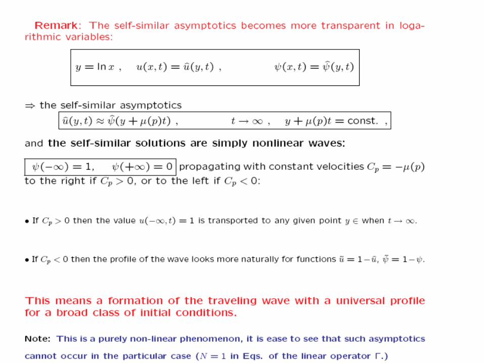
Self similar asymptotics for:

For any initial state φ(x) = 1 – xp + x(p+Є) , p ≤ 1. Decay rates in Fourier space: (p+Є)[ μ(p) - μ(p +Є) ]

For finite (p=1) or infinite (p<1) initial energy.

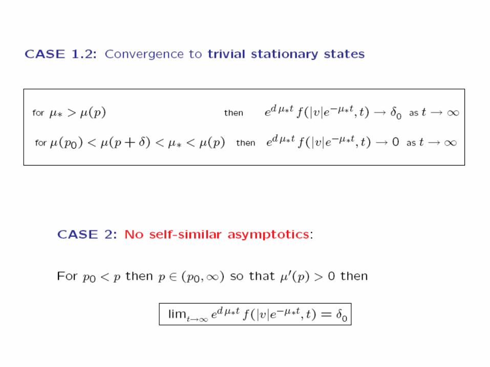
For p0< 1 and p=1

No self-similar asymptotics with finite energy

s*

For μ(1) = μ(s*) , s* >p0 >1

Power tailsCLT to a stable law

Finite (p=1) or infinite (p<1) initial energy

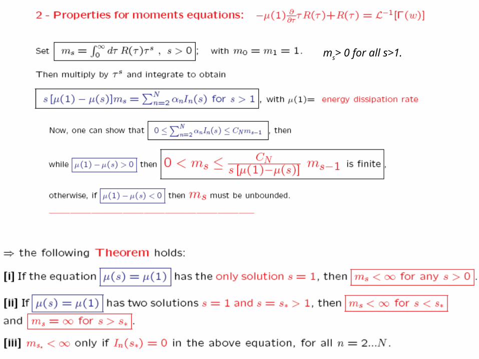
Study of the spectral function μ(p) associated to the linearized collision operator

p

)

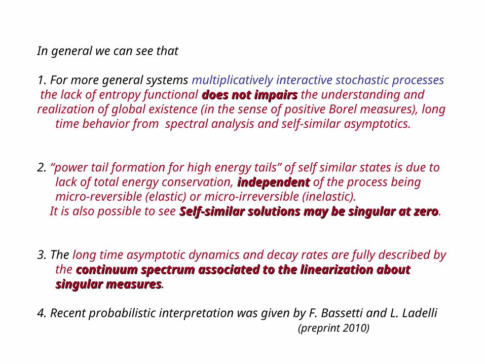
In general we can see that

1. For more general systems multiplicatively interactive stochastic processes the lack of entropy functional does not impairsdoes not impairs the understanding and realization of global existence (in the sense of positive Borel measures), long

time behavior from spectral analysis and self-similar asymptotics.

2. “power tail formation for high energy tails” of self similar states is due to lack of total energy conservation, independent independent of the process being micro-reversible (elastic) or micro-irreversible (inelastic).

It is also possible to see Self-similar solutions may be singular at zeroSelf-similar solutions may be singular at zero.

3. The long time asymptotic dynamics and decay rates are fully described by the continuum spectrum associated to the linearization about continuum spectrum associated to the linearization about singular measuressingular measures.

4. Recent probabilistic interpretation was given by F. Bassetti and L. Ladelli(preprint 2010)

with initial condition u|t=0 = e−x

Back to the Back to the M-game modelM-game model

Example of (a,b) pair choice: The game of j ≥ 1 players is played in three steps:

1- the participants collect all their goods and form a sum = v1 + v 2 + · · · + vj ;2- the sum is multiplied by a random number θ≥ 0 distributed with given probabilitydensity q(θ) in +;3- the resulting sum ’ = θ v′1 +· · ·+v′j is given back to the players in accordancewith the following rule: for some fixed or random parameter 0 ≤ ≤ 1.

• a part of it ’1 = (1- ’ is divided proportionally to initial contributions, • whereas the rest ′2 = ′ is divided among all players equally,Simple algebra shows that this “game” is equivalent to chose (a,b)

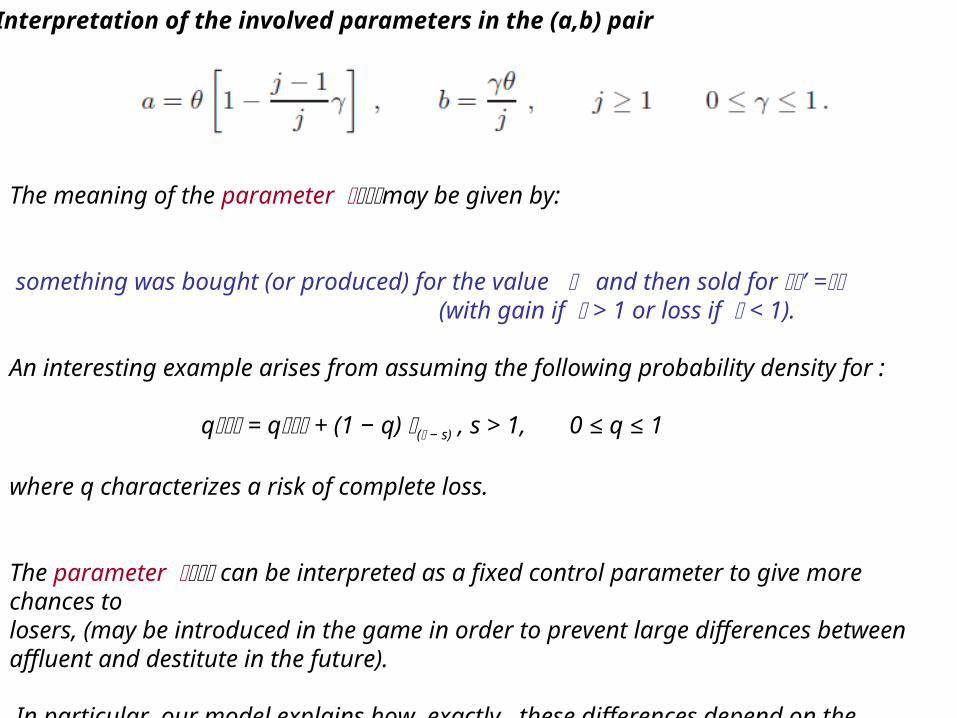
The meaning of the parameter may be given by:

something was bought (or produced) for the value and then sold for ′ = (with gain if > 1 or loss if < 1).

An interesting example arises from assuming the following probability density for : q = q + (1 − q) ( − s) , s > 1, 0 ≤ q ≤ 1

where q characterizes a risk of complete loss.

The parameter can be interpreted as a fixed control parameter to give more chances tolosers, (may be introduced in the game in order to prevent large differences betweenaffluent and destitute in the future).

In particular, our model explains how exactly these differences depend on the parameter .

Interpretation of the involved parameters in the (a,b) pair

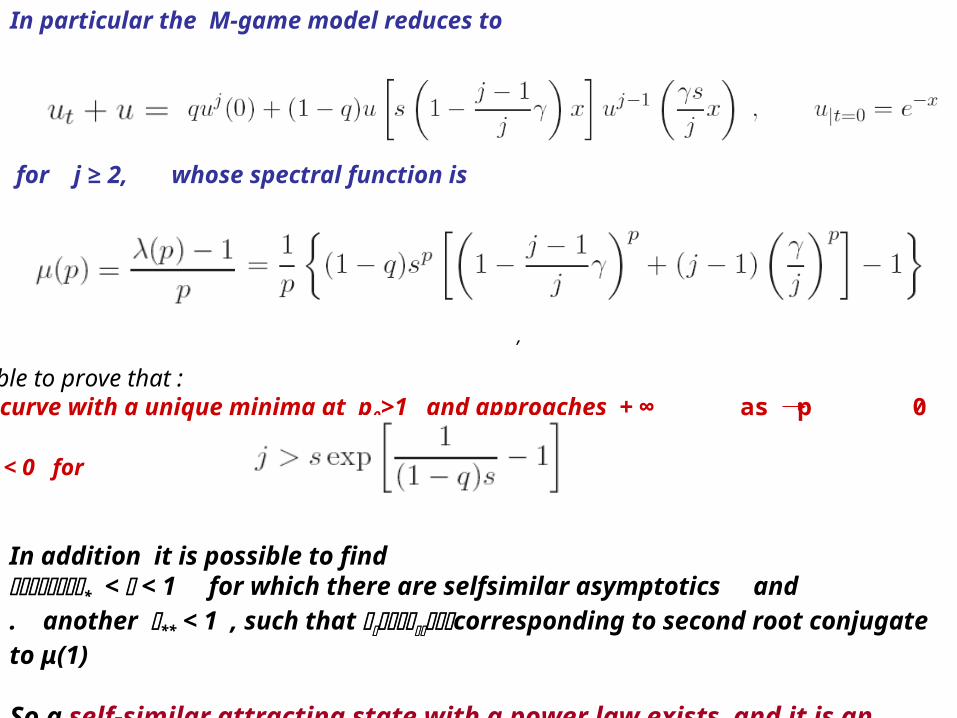
In particular the M-game model reduces to

,

It is possible to prove that : μ(p) is a curve with a unique minima at p0>1 and approaches + ∞ as p 0 and μ’(1) < 0 for

In addition it is possible to find * < < 1 for which there are selfsimilar asymptotics and . another ** < 1 , such that corresponding to second root conjugate to μ(1)

So a self-similar attracting state with a power law exists and it is an attractor

for j ≥ 2, whose spectral function is

Thank you very much for your attention

A.V. Bobylev, C. Cercignani and I. M. Gamba, On the self-similar asymptotics for generalized  non-linear kinetic Maxwell models, Comm. Math. Phys. 291 (2009), no. 3, 599--644.

A.V. Bobylev, C. Cercignani and I. M. Gamba, Generalized kinetic Maxwell models of granular gases; Mathematical models of granular matter Series: Lecture Notes in Mathematics Vol.1937, Springer, (2008) .

A.V. Bobylev, C. Cercignani and I. M. Gamba, On the self-similar asymptotics for generalized non-linear kinetic Maxwell models, arXiv:math-ph/0608035 A.V. Bobylev and I. M. Gamba, Boltzmann equations for mixtures of Maxwell gases: exact solutions and power like tails. J. Stat. Phys. 124, no. 2-4, 497--516. (2006).

A.V. Bobylev, I.M. Gamba and V. Panferov, Moment inequalities and high-energy tails for Boltzmann equations wiht inelastic interactions, J. Statist. Phys. 116, no. 5-6, 1651-1682.(2004).

A.V. Bobylev, J.A. Carrillo and I.M. Gamba, On some properties of kinetic and hydrodynamic equations for inelastic interactions, Journal Stat. Phys., vol. 98, no. 3?4, 743?773, (2000).

D. Duffie, S. Malamud, and G. Manso, Information Percolation with Equilibrium Search Dynamics, Econometrica, 2009.

D. Duffie, G. Giroux, and G. Manso, Information Percolation, preprint 2009

I.M. Gamba and Sri Harsha Tharkabhushaman, Spectral - Lagrangian based methods applied to computation of Non - Equilibrium Statistical States. Journal of Computational Physics 228 (2009) 2012–2036

I.M. Gamba and Sri Harsha Tharkabhushaman, Shock Structure Analysis Using Space Inhomogeneous Boltzmann Transport Equation, To appear in Jour. Comp Math. 09

And references therein