Extending the Root-Locus Method to Fractional-Order Systems

Hindawi Publishing CorporationJournal of Applied MathematicsVolume 2008, Article ID 528934, 13 pagesdoi:10.1155/2008/528934

Research ArticleExtending the Root-Locus Method toFractional-Order Systems

Farshad Merrikh-Bayat1 and Mahdi Afshar2

1Department of Electrical Engineering, Zanjan University, Zanjan, Iran2Department of Mathematics, Zanjan Azad University, Zanjan, Iran

Correspondence should be addressed to Farshad Merrikh-Bayat, [email protected]

Received 16 September 2007; Revised 11 March 2008; Accepted 14 May 2008

Recommended by Alberto Tesi

The well-known root-locus method is developed for special subset of linear time-invariant systemsknown as fractional-order systems. Transfer functions of these systems are rational functions withpolynomials of rational powers of the Laplace variable s. Such systems are defined on a Riemannsurface because of their multivalued nature. A set of rules for plotting the root loci on the firstRiemann sheet is presented. The important features of the classical root-locus method such asasymptotes, roots condition on the real axis, and breakaway points are extended to fractional case.It is also shown that the proposed method can assess the closed-loop stability of fractional-ordersystems in the presence of a varying gain in the loop. Three illustrative examples are presented toconfirm the effectiveness of the proposed algorithm.

Copyright q 2008 F. Merrikh-Bayat and M. Afshar. This is an open access article distributed underthe Creative Commons Attribution License, which permits unrestricted use, distribution, andreproduction in any medium, provided the original work is properly cited.

1. Introduction

The root-locus method of Evans is one of the most popular and powerful tools for bothanalysis and design of single-input single-output (SISO) linear time-invariant (LTI) systems.There are two main application areas for this method [1] as follows. (1) Stability: to obtainsufficient conditions on a real parameter k under which the closed-loop system in Figure 1remains stable. (2) Design: the root-locus method offers an efficient tool for design of lead-lagcompensators. There have been further advances to the root-locus method since its origin in1948. Krall [2, 3] developed the method for delayed systems, Bahar and Fitzwater [4] studiedthe problem from the numerical point of view and finally, Byrnes et al. [5] presented the root-locus method for distributed parameter systems.

For typical systems, there are several easy-to-use rules for plotting the root loci that donot generally suffice to determine it uniquely [1]. These rules serve only as hints and often the

mailto:[email protected]

2 Journal of Applied Mathematics

r k

−

+P(s) = yN(s)

D(s)

Figure 1: Standard closed-loop system.

intuitive insight of a control engineer is needed for completing the root-locus plot. The root-locus method will apparently become more difficult to apply as the system’s order becomeshigher [5].

In recent years, there has been an increasing attention to fractional-order systems. Thesesystems are of interest for both modelling and controller design purposes. In the fields ofcontinuous-time modelling, fractional derivatives have proved useful in linear viscoelasticity,acoustics, rheology, polymeric chemistry, biophysics, . . . [6, 7]. In general, fractional-ordersystems are useful to model various stable physical phenomena (commonly diffusive systems)with anomalous decay.

An interesting study of fractional differential systems appeared in [8] using a stochasticframework. The idea of fractional powers is also used for identification purposes. Tsao et al. [9]and Poinot and Trigeassou [10] clarify the identification method when the members of modelset are of fractional order. Two applications of such identifications can be found in [11, 12].Fractional-order systems are also used in control field. Podlubny [13] and Valerio and Sa daCosta [14] discussed methods of designing PIλDμ controllers, Raynaud and Zergaınoh [15]studied fractional-order lead-lag compensators, and Oustaloup et al. [16, 17] introduced theso-called CRONE controllers.

In this paper, the systems under consideration are described by rational transferfunctions and the powers of the Laplace variable, s, are limited to rational numbers. Suchsystems lend themselves well to some algebraic tools [18, 19]. Practical examples of suchsystems can be found in [11, 12, 19]. The problem of plotting the root loci for these systemsis treated in this paper. Unlike [5] that deals with infinite-dimensional systems, in the problemwe are going to solve, the systems are assumed to be of finite dimension and this makes theproblem simple enough to deal with analytically.

The proposed method can be used to examine whether a given closed-loop system, asshown in Figure 1, remains stable for large k’s or not, where P(s) is a fractional-order transferfunction. In [20], a generalization of the Routh-Hurwitz criterion for fractional-order systemsis presented. However, this method can deal with the stability problem for such systems but itis a very complicated algorithm.

The rest of this paper is arranged as follows. Section 2 provides some basic definitionsand notations together with the problem statement. In Section 3, the rules for plotting the rootloci in fractional case are presented. Three illustrative examples are presented in Section 4.Finally, some conclusions end the paper.

Notation

Blackboard capitals denote sets and spaces: especially N the natural numbers (without zero), Rthe real numbers, Q the rational numbers, Z the integer numbers, and C the complex numbers.The symbol �x�, where x ∈ R, denotes the biggest integer that is less than or equal to x.

F. Merrikh-Bayat and M. Afshar 3

2. Problem statement and preliminaries

Before introducing the main problem, some basic definitions and notations are provided. It isassumed that the reader is familiar with the concepts of “Riemann surface,” “Riemann sheet,”“branch point,” and “branch cut” (see, e.g., [21], or [22] for deeper analysis).

Definition 2.1. The function Q(s) = a1sq1 + a2s

q2 + · · · + ansqn is a fractional-order polynomial, if

and only if qi ∈ Q+ ∪ {0}, ai ∈ R, for i = 1, . . . , n.

Definition 2.2. Consider the fractional-order polynomial

Q(s) = a1sα1/β1 + a2s

α2/β2 + · · · + ansαn/βn , ai ∈ R, αi ∈ N ∪ {0}, βi ∈ N, (2.1)

where αi, βi are relatively prime for i = 1, . . . , n. (If for some i, αi = 0 then by definition βi = 1.)Let λ be the least common multiple (lcm) of β1, β2, . . . , βn denoted as λ = lcm{β1, β2, . . . , βn}.Then Q(s) can be written as

Q(s) = a1(s1/λ

)λ1 + a2(s1/λ

)λ2 + · · · + an

(s1/λ

)λn . (2.2)

Now the fractional degree (fdeg) of Q(s) is defined as

fdeg{Q(s)

}= max

{λ1, λ2, . . . , λn

}. (2.3)

The function Q as defined in (2.2) is a multivalued relation of s the domain of definitionfor which is a Riemann surface with λ Riemann sheets where the origin is a branch point [21].In this paper, the branch cut is assumed at R

− and the first Riemann sheet is denoted by P anddefined as

P :={reiθ | r > 0, − π < θ ≤ π

}. (2.4)

Note that each Riemann sheet has only one edge at branch cut. The following proposition givesthe roots number of Q(s) = 0.

Proposition 2.3. Let Q(s) be a fractional-order polynomial with fdeg{Q(s)} = n. Then the equationQ(s) = 0 has exactly n roots on the Riemann surface.

Proof. Consider

Q(s) = a1(s1/v

)n+ a2

(s1/v

)n−1+ · · · + an

(s1/v

)1+ an+1, (2.5)

for an appropriate v ∈ N. Assuming w := s1/v, we have

Q(w) = a1wn + a1w

n−1 + · · · + anw + an+1. (2.6)

The fundamental theorem of algebra gives n roots for Q(w) = 0, say w1, w2, . . . , wn. Con-sequently, Q(s) = 0 has n roots at s1 = wv

1 , s2 = wv2 , . . . , sn = wv

n.


Definition 2.4. The fractional-order polynomial Q(s) = a0sn/v + a1s

(n−1)/v + · · · + an−1s1/v + an isminimal if fdeg{Q(s)} = n.

Now consider the standard closed-loop system in Figure 1 where the transfer functionof plant is given by

P(s) =N(s)D(s)

=sm/v + b1s

(m−1)/v + · · · + bm−1s1/v + bmsn/v + a1s(n−1)/v + · · · + an−1s1/v + an

, (v > 1), (2.7)

and k is assumed to be a positive real constant. Note that the domain of definition of P(s) is aRiemann surface with v Riemann sheets [21].

Definition 2.5. With the above notations, P(s) is called strictly proper for n > m, proper forn ≥ m, nonproper for n < m, and biproper for n = m.

Definition 2.6. The roots of the equations N(s) = 0 and D(s) = 0 on P are called open-loopzeros and open-loop poles, respectively.

It is a fact that when a minimal fractional-order polynomial is represented in anonminimal form, the number of its zeros is increased but the location and the order of zerosonP remain unchanged. For example, consider the fractional-order polynomials f(s) = s1/2−1(minimal) and g(s) = s2/4 − 1 (nonminimal). The equation f(s) = 0 has only one root at s = ei0

(on the first Riemann sheet)while g(s) = 0 has a root at s = ei0 (on the first Riemann sheet), andanother root at s = ei4π (on the third Riemann sheet), although f(s) and g(s) have differentnumber of zeros but the location and the order of their zero on P are identical. It concludesthat Definition 2.6 is not ambiguous; representing N(s) and D(s) in a nonminimal form willnot affect the open-loop poles and zeros.

Note that s = 0 is not a pole of P(s) even ifD(0) = 0. The following definition deals withthe singularities at the origin.

Definition 2.7. The point s = 0 is defined to be a pole of order r of P(s) (as defined in (2.7)) ifthe point w = 0 is a pole of order r of P(w) := P(s) |w=s1/v .

The characteristic equation of the closed-loop system shown in Figure 1 is

Δ(s) = D(s) + kN(s)

= sn/v + a1s(n−1)/v + · · · + an−1s1/v + an + k

[sm/v + b1s

(m−1)/v + · · · + bm−1s1/v + bm]= 0.(2.8)

It is desired to address the generalized root-locus problem that is to plot the root loci of (2.8)on P when k varies. The reason for concerning about the first Riemann sheet is that the time-domain behavior and stability properties of the closed-loop system are determined only bythose roots of the characteristic equation that lie on the first Riemann sheet [19, 23]. Note that asystem with characteristic equation (2.8) is stable (in the sense of bounded-input bounded-output) if and only if it has no roots in the closed right half plane (CRHP) of P [24, 25].


Sheet v

Im w

Sheet 2

Sheet 1

Re wπ/v

· · ·

· · ·

Figure 2: The correspondence between w-plane and s Riemann sheets.

In this paper, we restrict ourselves to the following conditions.

(i) The transfer function of the plant is strictly proper. Final results can easily beextended for nonproper systems but such an extension to biproper transfer functionsis complicated. This is similar to the difficulty that occurs when the root-locus plot foran integer-order system with biproper transfer function is involved [26].

(ii) Parameter k is a positive real number. The results can easily be extended for negativereal k’s.

(iii) Both N(s) and D(s) are monic fractional-order polynomials. This does not lose thegenerality and simplifies the notations.

(iv) N(s) and D(s) have no common roots. Otherwise, the characteristic equation willhave root(s) that does (do) not vary by changing k.

In the rest of this paper, the single-valued function obtained by replacing every s1/v in (2.8)with w is denoted by Δ(w), that is,

Δ(w) = wn + a1wn−1 + · · · + an−1w + an + k

[wm + b1w

m−1 + · · · + bm−1w + bm]= 0. (2.9)

We do the same for other multivalued relations.

3. Root loci in fractional case

3.1. Properties of the root loci in fractional case

The root-locus plot of Δ(w) = 0 provides a very good insight to the root-locus plot of Δ(s).Figure 2 shows the relationship between w-plane and sheets of the s Riemann surface. In thisfigure, the sector −π/v < argw ≤ π/v corresponds to P. In the following, some importantfeatures of the root loci of Δ(s) are presented.


3.1.1. Symmetry with respect to real axis

Considering the fact that the root loci of Δ(w) = 0 is symmetric with respect to real axis, it isconcluded that the roots loci of Δ(s) on P are also symmetric with respect to real axis. Notethat, in general, this explanation is not correct for the root loci on other Riemann sheets.

3.1.2. Number of branches

A branch by definition is the loci of a single root of the characteristic equation when k variesfrom zero to infinity. In classical case, the root-locus branches start from open-loop poles andterminate at zeros (finite zeros or zeros at infinity) [1]. In fractional case, it is concluded fromProposition 2.3 that the characteristic equation (2.8) has n roots distributed on v Riemannsheets. Considering the root-locus plot of Δ(w) in w-plane, it is obvious that not all root-locusbranches on necessarily start from open-loop poles and terminate at open-loop zeros. In fact, abranch may cross the branch cut and enter to another Riemann sheet.

There is another point that should be noted here. Clearly, r branches start from the open-loop pole s0 ∈ P which is of order r. When s0 /∈R

−, all these branches are on P for k→ 0+.Otherwise, they belong to different Riemann sheets. One important case is due to the poles atthe origin. If s1 = 0 is a pole of order r of (2.7), then r branches start it, which are not necessarilyon for k→ 0+. In order to find the number of branches that start from s1 and are onP for k→ 0+,let p and q stand for the number of positive real open-loop poles and zeros, respectively. Thenaccording to the angle condition, the angle of departure from the pole at the origin is obtainedas

φh =2h + 1 − p + q

rvπ, h =

⌊p − q − (n/v) − 1

2

⌋+ 1, . . . ,

⌊p − q + (n/v) − 1

2

⌋. (3.1)

As a result, if (2.7) has a pole of order r at the origin, then �(p − q + (n/v) − 1)/2� − �(p − q −(n/v) − 1)/2� branches (on P) start from s = 0 the angle of departure of which is calculatedfrom (3.1).

3.1.3. Roots conditions on the real axis

In the classical root-locus algorithm, any point on the real axis, the total number of real polesand zeros to the right of which is odd, lies on a root locus. Clearly, the line segments lying onthe positive real axis ofw-plane are mapped to the line segments lying on the positive real axisof P. So, according to the root-locus plot in w-plane, any point on the positive real axis of P,the total number of real poles and zeros to the right of which is odd, lies on a root locus. Butfor P(s) given in (2.7), no line segment on R

− can belong to the root locus. The reason is asfollows. If such a line exists then it should necessarily lie on the ray reiπ/v (r > 0) in w-plane.It is a well-known classical result that the semiinfinite line reiπ/v (r > v

√x), which is a root loci

branch of a systemwith transfer function P(w) = (1/(wv +x)) (x ∈ R+), is the only object inw-

plane that can lie on this ray. But P(w) corresponds to P(s) = 1/((s1/v)v +x) = 1/(s+x)whichis not multivalued. Consequently, the root-locus plot of the multivalued transfer function P(s)can never have a branch at R

−.


3.1.4. Asymptotes and their directions

Asymptotes are very important in drawing a root-locus plot as they exhibit directions of thebranches for large k’s. The asymptotes of the root-locus plot in integer case are first studied in[21]. Another explanationwithmore details can be found in [27]. The approach used in [21, 27]cannot directly be applied for fractional case. Here we develop an alternative approach to findthe asymptotes to the root-locus curves of a fractional-order transfer function. The followingtheorem is the main result of this paper because it can be used to examine the closed-loopstability for large gains.

Theorem 3.1. Asymptotes of the root-locus plot are straight lines all passing through the origin andtheir directions are given by

ϕh =(2h + 1)vn −m

180◦, h =⌊m − n − v

2v

⌋+ 1, . . . ,

⌊m − n − v

2v

⌋+ n −m. (3.2)

Proof. See Appendix.

Note that in Theorem 3.1, h may belong to any sequence of n − m successive integernumbers but the sequencewe have usedmakes a relevant correspondence between asymptotesand Riemann sheets. This sequence guarantees that −180◦ < ϕh< 360◦v − 180◦. Note also thatfor h = �(m−n−v)/2v�+1, . . . , �(n−m−v)/2v� the resulting asymptotes lie on P. In fractionalcase, however, all asymptotes pass through the origin. Since the open-loop system is assumedto be strictly proper, the root-locus plot will always have at least one asymptote.

Remark 3.2. In integer case, if the negative real axis is an asymptote for the root-locus plot,then it is the asymptote for one and only one of the branches. Moreover, the correspondingbranch of the root-locus plot coincides with the asymptote. In the fractional case, however, thenegative real axis can be an asymptote line for more than one root and it is not superposed onany branch. As a matter of fact, according to (3.2) the negative real axis is the asymptote for allinfinite roots when n −m = v.

3.1.5. Breakaway and break-in points

The breakaway and break-in points on a root-locus plot are points where two or more branchesintersect and then go apart. If s0 is a breakaway (break-in) point then it necessarily satisfiesboth Δ(s0) = 0 and dΔ(s0)/ds = 0 for some s0 on P. These two equations imply thatD(s0) + kN(s0) = 0 and dD(s0)/ds + kdN(s0)/ds = 0 or equivalently, N(s0)dD(s0)/ds −D(s0)dN(s0)/ds = 0. The latter equation can be interpreted in terms of the open-loop transferfunction, P(s), as dP(s0)/ds = 0. So, every breakaway (break-in) point must satisfy theequation

dP(s)ds

= 0, (3.3)

on P (see, e.g., [21] for differentiation of multivalued relations). The roots of (3.3) arebreakaway (break-in) points if the corresponding k ’s are positive real numbers. Equation (3.3)can also be interpreted in terms of P(w) as dP(w)/dw = 0.


3.2. Comprehensive algorithm

The following is a summarization of the general rules for constructing the root loci in fractionalcase.

(1) Locate the open-loop poles and zeros.

(2) Determine the order of the pole at the origin (if any) and calculate the angle ofdeparture using (3.1).

(3) Determine the root loci on the positive real axis. Note that no line segment on thenegative real axis can belong to the root loci.

(4) Determine the directions of asymptotes from (3.2).

(5) Find the breakaway and break-in points (in any) from (3.3).

(6) Complete the root-locus plot.

4. Examples

Example 4.1. Consider the closed-loop system in Figure 1 with

P(s) =s1/2 − 1

s2 − 3s3/2 − 2s + 2s1/2 + 12. (4.1)

The open-loop poles of this system are located at s = 4ei0 and s = 9ei0, and there is an open-loop zero located at s = 1ei0. The line segments 0 ≤ R{s} ≤ 1 and 4 ≤ R{s} ≤ 9 belong tothe root loci because the total number of poles and zeros to the right of any point on them isan odd number. The directions of the asymptotes (on the first Riemann sheet) are ϕ−1 = −120◦and ϕ0= 120◦. The roots of the equation dP(w)/dw are 2.4820, −0.9599, and 0.9056 ± i1.0671.The only feasible solution isw = 2.4820 which corresponds to s = 6.1603ei0. Figure 3 shows theroot-locus plot of this system.

Example 4.2. Consider the closed-loop system in Figure 1 with

P(s) =s1/2 − √

2

s2(s1/2 − 1

)3 . (4.2)

This system has an open-loop zero at s = 2ei0 and an open-loop pole of order three at s = 1ei0.There is also a pole of order four at the origin. The line segment 1 ≤ R{s} ≤ 2 on the positivereal axis belongs to the root loci. According to (3.1), the angles of departure from the pole atthe origin are φ0 = −π/2 and φ1 = π/2. Letting n = 7, m = 1, and v = 2, it is concluded from(3.2) that the directions of the asymptotes on P are ϕ−1 = −60◦, ϕ0= 60◦, and ϕ1= 180◦. Figure 4shows the root-locus plot of this system.

Example 4.3. According to [28], the fractional-order model of a heating furnace is given by

P(s) =1

14994s1.131 + 6009.5s0.97 + 1.69, (4.3)


−25

−20

−15

−10

−5

0

5

10

15

20

25

Im{s}

−5 0 5 10 15

Re{s}

Figure 3: Root-locus plot of Example 4.1.

−2

−1.5

−1

−0.5

0

0.5

1

1.5

2

Im{s}

−1.5 −1 −0.5 0 0.5 1 1.5 2

Re{s}

Figure 4: Root-locus plot of Example 4.2.

which compared to (2.7) results in n = 131, m = 0, and v = 100. Assuming P(s) in theconnection of Figure 1, the root-locus plot has two asymptotes on the directions of which areϕ−1 ≈ −137.4◦ and ϕ0 ≈ 137.4◦, thanks to (3.2). Since none of these asymptotes lie on theCRHP of P and P(s) has no zeros, one can choose k arbitrarily large to arrive at a closed-loop system with the ability of tracking the command input. Figure 5 shows the closed-loopsystem response for k = 5, 10, 20 together with the open-loop system response when the systemis subjected to a unit step. As it is expected, the closed-loop system is stable and its bandwidthis increased by increasing k. Podlubny [29] proposed the fractional-order model

P(s) =1

0.7943s2.5708 + 5.2385s0.8372 + 1.5560, (4.4)


0

0.5

1

0 0.5 1 1.5 2 2.5 3×104

Time (s)

Open-loopk = 5

k = 10k = 20

Figure 5: Step responses corresponding to Example 4.3.

for another heating furnace. This transfer function can be represented in the equivalent form

P(s) =1

0.7943s6427/2500 + 5.2385s2093/2500 + 1.5560, (4.5)

which corresponds to n = 6427,m = 0, and v = 2500. The root-locus plot of this system has twounstable infinite branches the directions of which are ϕ−1 ≈ −70.02◦ and ϕ0 ≈ 70.02◦. Hence,it is not possible to control the system by means of a simple proportional action. One possibleapproach is to use more complex structures such as lead-lag compensators.

5. Conclusion

In this paper, an approach for constructing the root-locus plot for fractional-order systems isdeveloped. Important features of the root loci are studied and a comprehensive algorithm ispresented. Although the rules for plotting the root loci in fractional case are somehow similar tothose available in integer case, there are also some major differences. For example, it is shownthat in fractional case no line segment on R

− can belong to the root loci. It is also shown that theasymptotes of all infinite branches of the root-locus plot pass through the origin. As anotherdifference, the well-known Routh-Hurwitz stability test cannot be used to find the points atwhich the root-locus plot intersects with the imaginary axis. Three illustrative examples arepresented to confirm the effectiveness of the proposed algorithm.

Appendix

The following is a proof for Theorem 3.1. Consider the general form of the characteristicequation as follows:

1 + ksm/v + b1s

(m−1)/v + · · · + bmsn/v + a1s(n−1)/v + · · · + an

= 0, (A.1)

which can be written as

sn/v + a1s(n−1)/v + · · · + an

sm/v + b1s(m−1)/v + · · · + bm= −k, (A.2)

then

s(n−m)/v(1 +

a1 − b1sv

+ · · ·)

= −k, (A.3)


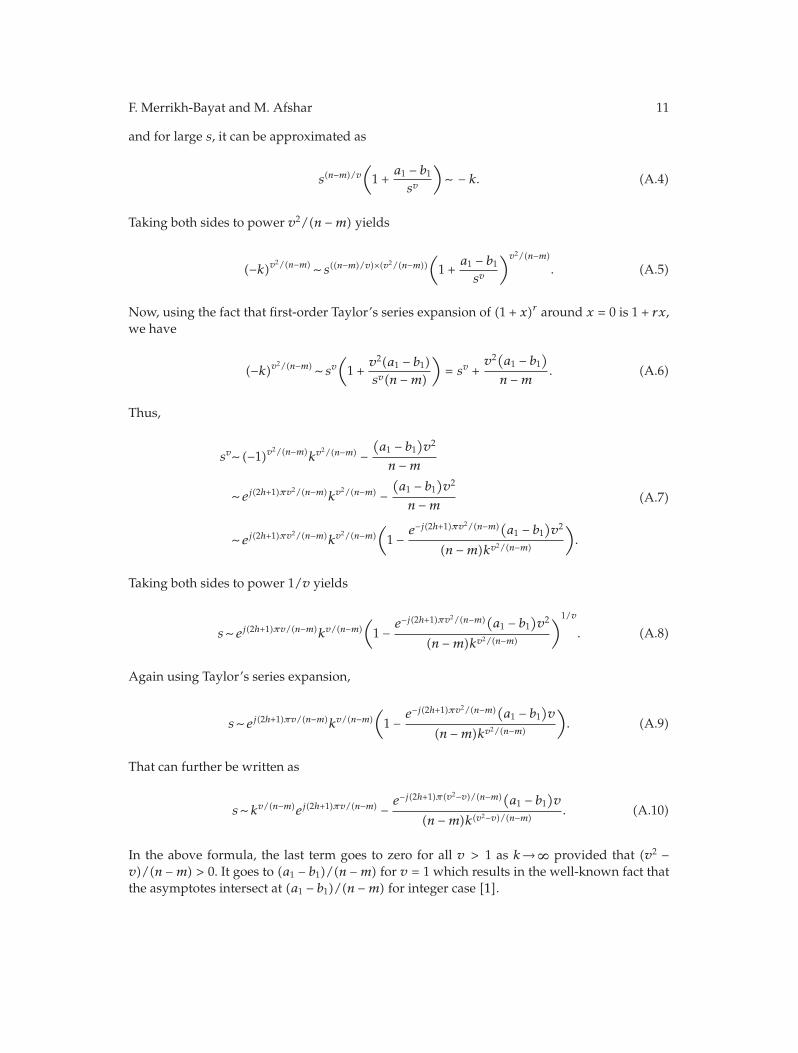
and for large s, it can be approximated as

s(n−m)/v(1 +

a1 − b1sv

)∼ − k. (A.4)

Taking both sides to power v2/(n −m) yields

(−k)v2/(n−m) ∼ s((n−m)/v)×(v2/(n−m))(1 +

a1 − b1sv

)v2/(n−m)

. (A.5)

Now, using the fact that first-order Taylor’s series expansion of (1 + x)r around x = 0 is 1 + rx,we have

(−k)v2/(n−m) ∼ sv(1 +

v2(a1 − b1)sv(n −m)

)= sv +

v2(a1 − b1)

n −m. (A.6)

Thus,

sv∼ (−1)v2/(n−m)kv2/(n−m) −(a1 − b1

)v2

n −m

∼ ej(2h+1)πv2/(n−m)kv2/(n−m) −

(a1 − b1

)v2

n −m

∼ ej(2h+1)πv2/(n−m)kv2/(n−m)

(1 − e−j(2h+1)πv

2/(n−m)(a1 − b1)v2

(n −m)kv2/(n−m)

).

(A.7)

Taking both sides to power 1/v yields

s∼ ej(2h+1)πv/(n−m)kv/(n−m)(1 − e−j(2h+1)πv

2/(n−m)(a1 − b1)v2

(n −m)kv2/(n−m)

)1/v

. (A.8)

Again using Taylor’s series expansion,

s∼ ej(2h+1)πv/(n−m)kv/(n−m)(1 − e−j(2h+1)πv

2/(n−m)(a1 − b1)v

(n −m)kv2/(n−m)

). (A.9)

That can further be written as

s∼ kv/(n−m)ej(2h+1)πv/(n−m) − e−j(2h+1)π(v2−v)/(n−m)(a1 − b1

)v

(n −m)k(v2−v)/(n−m). (A.10)

In the above formula, the last term goes to zero for all v > 1 as k→∞ provided that (v2 −v)/(n −m) > 0. It goes to (a1 − b1)/(n −m) for v = 1 which results in the well-known fact thatthe asymptotes intersect at (a1 − b1)/(n −m) for integer case [1].


References

[1] K. Ogata,Modern Control Engineering, Prentice-Hall, Upper Saddle River, NJ, USA, 4th edition, 2001.[2] A. M. Krall, “The root locus method: a survey,” SIAM Review, vol. 12, no. 1, pp. 64–72, 1970.[3] A. M. Krall, “A closed expression for the root locus method,” SIAM Journal on Applied Mathematics,

vol. 11, no. 3, pp. 700–704, 1963.[4] E. Bahar andM. Fitzwater, “Numerical technique to trace the loci of the complex roots of characteristic

equations,” SIAM Journal on Scientific and Statistical Computing, vol. 2, no. 4, pp. 389–403, 1981.[5] C. I. Byrnes, D. S. Gilliam, and J. He, “Root-locus and boundary feedback design for a class of

distributed parameter systems,” SIAM Journal on Control and Optimization, vol. 32, no. 5, pp. 1364–1427, 1994.

[6] K. B. Oldham and J. Spanier, The Fractional Calculus: Theory and Applications of Differentiation andIntegration to Arbitrary Order, Academic Press, New York, NY, USA, 1974.

[7] R. Hilfe, Ed., Applications of Fractional Calculus in Physics, World Scientific, River Edge, NJ, USA, 2000.[8] M.-C. Viano, C. Deniau, and G. Oppenheim, “Continuous-time fractional ARMA processes,” Statistics

& Probability Letters, vol. 21, no. 4, pp. 323–336, 1994.[9] Y.-Y. Tsao, B. Onaral, and H. H. Sun, “An algorithm for determining global parameters of minimum-

phase systems with fractional power spectra,” IEEE Transactions on Instrumentation and Measurement,vol. 38, no. 3, pp. 723–729, 1989.

[10] T. Poinot and J.-C. Trigeassou, “Identification of fractional systems using an output-error technique,”Nonlinear Dynamics, vol. 38, no. 1–4, pp. 133–154, 2004.

[11] B. M. Vinagre, V. Feliu, and J. J. Feliu, “Frequency domain identification of a flexible structure withPiezoelectric actuators using irrational transfer function models,” in Proceedings of the 37th IEEEConference on Decision and Control (CDC ’98), vol. 2, pp. 1278–1280, Tampa, Fla USA, December 1998.

[12] A. Chauchois, D. Didier, A. Emmanuel, and D. Bruno, “Use of noninteger identification models formonitoring soil water content,”Measurement Science and Technology, vol. 14, no. 6, pp. 868–874, 2003.

[13] I. Podlubny, “Fractional-order systems and PIλDμ-controllers,” IEEE Transactions on Automatic Control,vol. 44, no. 1, pp. 208–214, 1999.

[14] D. Valerio and J. Sa da Costa, “Tuning of fractional PID controllers with Ziegler-Nichols-type rules,”Signal Processing, vol. 86, no. 10, pp. 2771–2784, 2006.

[15] H.-F. Raynaud and A. Zergaınoh, “State-space representation for fractional order controllers,”Automatica, vol. 36, no. 7, pp. 1017–1021, 2000.

[16] A. Oustaloup, B. Mathieu, and P. Lanusse, “The CRONE control of resonant plants: application to aflexible transmission,” European Journal of Control, vol. 1, no. 2, pp. 113–121, 1995.

[17] A. Oustaloup, X. Moreau, and M. Nouillant, “The CRONE suspension,” Control Engineering Practice,vol. 4, no. 8, pp. 1101–1108, 1996.

[18] K. S. Miller and B. Ross, An Introduction to the Fractional Calculus and Fractional Differential Equations, AWiley-Interscience Publication, John Wiley & Sons, New York, NY, USA, 1993.

[19] H. Beyer and S. Kempfle, “Definition of physically consistent damping laws with fractionalderivatives,” Zeitschrift fur Angewandte Mathematik und Mechanik, vol. 75, no. 8, pp. 623–635, 1995.

[20] M. Ikeda and S. Takahashi, “Generalization of Routh’s algorithm and stability criterion for non-integerintegral system,” Electronics and Communications in Japan, vol. 60, no. 2, pp. 41–50, 1977.

[21] W. R. LePage, Complex Variables and the Laplace Transform for Engineers, International Series in Pure andApplied Mathematics, McGraw-Hill, New York, NY, USA, 1961.

[22] G. A. Jones and D. Singerman, Complex Functions: An Algebraic and Geometric Viewpoint, CambridgeUniversity Press, Cambridge, UK, 1987.

[23] B. Gross and E. P. Braga, Singularities of Linear System Functions, Elsevier, New York, NY, USA, 1961.[24] D. Matignon, “Stability properties for generalized fractional differential systems,” in Systemes

Differentiels Fractionnaires (Paris, 1998), vol. 5 of ESAIM Proceedings, pp. 145–158, SMAI, Paris, France,1998.

[25] D. Matignon, “Stability results on fractional differential equations with applications to controlprocessing,” in Proceedings of the Computational Engineering in Systems Applications, CESA96 IMACS-IEEE/SMC Multiconference, pp. 963–968, Lille, France, July 1996.


[26] A. M. Eydgahi and M. Ghavamzadeh, “Complementary root locus revisited,” IEEE Transactions onEducation, vol. 44, no. 2, pp. 137–143, 2001.

[27] G. Berman and R. G. Stanton, “The asymptotes of the root locus,” SIAM Review, vol. 5, no. 3, pp.209–218, 1963.

[28] I. Podlubny, L. Dorcak, and I. Kostial, “On fractional derivatives, fractional order dynamic system andPIλDμ-controllers,” in Proceedings of the 36th IEEE Conference on Decision and Control (CDC ’97), vol. 5,pp. 4985–4990, San Diego, Calif, USA, December 1997.

[29] I. Podlubny, Fractional Differential Equations: An Introduction to Fractional Derivatives, FractionalDifferential Equations, to Methods of Their Solution and Some of Their Applications, vol. 198 of Mathematicsin Science and Engineering, Academic Press, San Diego, Calif, USA, 1999.

Submit your manuscripts athttp://www.hindawi.com

Hindawi Publishing Corporationhttp://www.hindawi.com Volume 2014

MathematicsJournal of


Mathematical Problems in Engineering

Hindawi Publishing Corporationhttp://www.hindawi.com

Differential EquationsInternational Journal of

Volume 2014

Applied MathematicsJournal of


Probability and StatisticsHindawi Publishing Corporationhttp://www.hindawi.com Volume 2014

Journal of


Mathematical PhysicsAdvances in

Complex AnalysisJournal of


OptimizationJournal of


CombinatoricsHindawi Publishing Corporationhttp://www.hindawi.com Volume 2014

International Journal of


Operations ResearchAdvances in

Journal of


Function Spaces

Abstract and Applied AnalysisHindawi Publishing Corporationhttp://www.hindawi.com Volume 2014

International Journal of Mathematics and Mathematical Sciences


The Scientific World JournalHindawi Publishing Corporation http://www.hindawi.com Volume 2014


Algebra

Discrete Dynamics in Nature and Society



Decision SciencesAdvances in

Discrete MathematicsJournal of

Hindawi Publishing Corporationhttp://www.hindawi.com

Volume 2014 Hindawi Publishing Corporationhttp://www.hindawi.com Volume 2014

Stochastic AnalysisInternational Journal of

Extending the Root-Locus Method to Fractional-Order Systems

Documents

Transcript of Extending the Root-Locus Method to Fractional-Order Systems