Centre for the Analysis of Risk

and Optimisation

Modelling Applications

A multi-disciplinary research centre focussed on understanding, modelling quantification,

management and control of RISK ,

TECHNICAL REPORT

CTR/09/03 November Extending algebraic modelling languages for Stochastic Programming Patrick Valente, Gautam Mitra and M Sadki Brunel University, Uxbridge, Middlesex R Fourer Northwester University, Evanston, IL

Department of Mathematical Sciences and

Department of Economics and Finance

Brunel University, Uxbridge, Middlesex, UB8 3PH

www.carisma.brunel.ac.uk

Extending algebraic modelling languages for Stochastic Programming

P. Valente, G. Mitra, M. Sadki

Brunel University, Uxbridge, Middlesex, UK

R. Fourer

Northwestern University, Evanston, IL

Abstract The algebraic modelling languages (AML) have gained wide acceptance and use in Mathematical

Programming by researchers and practitioners. At a basic level, stochastic programming models can

be defined using these languages by constructing their deterministic equivalent. Unfortunately, this

leads to very large model data instances. We propose a direct approach in which the random values

of the model coefficients and the stage structure of the decision variables and constraints are

"overlaid" on the underlying deterministic (core) model of the SP problems. This leads not only to a

natural definition of the SP model: the resulting generated instance is also a compact representation

of the otherwise large problem data. The proposed constructs enable the formulation of two stage

and multistage scenario based recourse problems, as well as chance constrained problems. This

design is presented as a stochastic extension of the AMPL language which we call SAMPL.

Table of Contents

1 Introduction.............................................................................................................2 1.1 Background .................................................................................................................2

2 Modelling stochastic programming problems..........................................................3 2.1 Taxonomy of SP models..............................................................................................3 2.2 Distribution problems..................................................................................................4 2.3 Stochastic Programming Problems with Recourse .....................................................5 2.4 Chance-Constrained Problems....................................................................................8

3 An illustrative example ...........................................................................................9 3.1 A deterministic network distribution model................................................................9 3.2 Introducing scenarios ................................................................................................ 12 3.3 Stochastic programming formulations ...................................................................... 15

4 Adapting algebraic modelling languages for SP...................................................18 4.1 Proposed approaches................................................................................................. 18 4.2 Analysis of modelling issues...................................................................................... 20 4.3 Overview of our approach.......................................................................................... 22 4.4 SAMPL language extensions..................................................................................... 24 4.5 Implementation of the illustrative examples in SAMPL ........................................... 31

5 Implementation of the language extensions...........................................................34 5.1 Interfacing modelling systems and solvers ............................................................... 34 5.2 Communicating with scenario generators................................................................. 37 5.3 Integrated environments: SPInE............................................................................... 40

6 Conclusions and directions for future research......................................................41

7 References ..............................................................................................................43

1

1 Introduction

1.1 Background

Over the past decades, stochastic programming models have gained wide acceptance by practitioners

in the field of optimisation and operations research. Research in financial areas such as portfolio

management and pension funds management (Ziemba and Mulvey 1998), in manufacturing networks

and supply chain optimisation (Eppen, Martin et al. 1989; Lucas, Messina et al. 1997; Escudero,

Galindo et al. 1999; Shapiro 2001), as well as in energy and environmental planning (Pereira and

Pinto 1985; Bosetti, Messina et al. 2002), has demonstrated that the solution of stochastic

programming models is superior to that of deterministic models in terms of expectation over future

events. Indeed, stochastic programming models explicitly consider uncertainty in some of the model

parameters, and provide optimal decisions which are hedged against such uncertainty.

Unfortunately, the size of stochastic programming problems grows exponentially with the number of

decision stages considered by the models and with the number of possible outcomes of the random

parameters at each stage. This is a challenging issue both in terms of modelling and solution

algorithms. The implementation of large scale mathematical programming models implies the

generation of matrices which represent the problem constraints and are stored in machine readable

form in order to be interpreted by the solvers. This generation process used to be performed by ad-

hoc software modules, and required considerable development effort. For deterministic models, the

evident drawbacks of this approach were overcome with the advent of a class of declarative

programming languages known as Algebraic Modelling Languages (AML), which represent powerful and

flexible instruments for the generation of model data instances. The entities of the optimisation

models (sets, decision variables, parameters, constraints, objectives etc.) are defined in a way that

closely resembles the algebraic notation. AMPL (Fourer, Gay et al. 1993), GAMS (Brooke, Kendrick

et al. 1998), AIMMS (Bisschop and Roelofs 1999) and MPL (Maximal Software 2002) are amongst

the most commonly used AMLs. Most of these support the formulation of Linear Programs (LP),

Mixed Integer Programs (MIP), Quadratic Programs (QP) and recently Non Linear Programs (NLP),

and are capable of generating model instances using machine readable formats.

Stochastic programming models are characterised by the presence of uncertainty associated with

some of their parameters, which therefore become random variables with a specified probability

distribution. Unfortunately, the existing modelling languages do not provide appropriate constructs

for the definition of this random nature. In this report we present a direct approach for the definition

of SP models via declarative syntax, and illustrate how this idea can be applied to extend virtually any

2

algebraic modelling language. We consider the AMPL systems and by means of examples, define the

syntax of the stochastic extension SAMPL.

The rest of the report is organised as follows:

In section 2, we define various classes of models for optimum decision making under uncertainty. In

section 3 we introduce an illustrative model which we first formulate as a linear program, and then

extend into a two stage and multistage stochastic programming problem with recourse, and finally

into a chance constrained problem. In section 4, we analyse the modelling requirements for

stochastic programming problems and introduce our approach in extending algebraic modelling

languages. We define new language constructs for AMPL and use the resulting SAMPL extension to

formulate the illustrative model. In section 5 we consider the practical implementation of these

stochastic programming extensions; in particular, we focus on the integration of algebraic modelling

systems with scenario generators and solution methods. We conclude in section 6 with some final

remarks and future research directions.

2 Modelling stochastic programming problems

2.1 Taxonomy of SP models

There is a growing body of literature covering many applications of SP (see Annals of Operations

Research, 1999 vol. 85). In this section we consider the family of models which is now well

established and come under the broad heading of optimum decision making under uncertainty. We

follow the classification of stochastic programming problems introduced by (Gassmann and Ireland

1996). We make a small extension of their categorisation by adding the Expected Value models as a

subclass of the distribution problems leading to a working taxonomy shown in Figure 1.

SP problems

Chance Constrained

Problems

Recourse Problems

Distribution Problems

Scenario-based

Distribution-based

Wait and See Expected Value

Stochastic Measures: EVPI and VSS

Figure 1 Taxonomy of SP problems.

3

We illustrate these classes by first considering the linear programming problem:

mnnm RbRxcRAwherex

bAxtosubjectcxZ

;,;0

min

(1)

Let (, F, P) denote a (discrete) probability space where denote the events. Let us denote the

realizations of A, b, c for a given as:

orcbA ,, (2)

We use pω = p(ξ()) to denote the probability associated with the realisation ξ(). The classes of

stochastic models illustrated in Figure 1 are defined in the following sections.

2.2 Distribution problems

The distribution of the objective function value for different realisations of the random parameters

and also for the expected value of such parameters are broadly known as the distribution problems.

The Expected Value Problem

The Expected Value (EV) model is constructed by replacing the random parameters by their

expected values. Such EV model is thus a linear program, as the uncertainty is dealt with before it is

introduced into the underlying linear optimisation model. It is common practice to formulate and

solve the EV problem in order to gain some insight into the decision problem. Let the constraint sets

corresponding to the problem stated in (1) be defined as:

orcbAforxbxAxF ,,0,| (3)

We can reconsider (1) as an expected value or an average value problem where:

bxA

tosubjectxcZ

pEcbA

EV

min

),,(

(4)

4

Let x*ev denote the optimal solution to the above problem. This solution can be evaluated for all

possible realisations . We can thus determine the corresponding objective function values and

compute what is called the expectation of the expected value solution:

*evEEV xcEZ

(5)

If, however, an ω exists such that: x*ev F, i.e. x*ev is not feasible for some realisations of the random

parameters, we set:

EEVZ (6)

Wait and See Problems

Wait and See (WS) problems assume that the decision-maker is somehow able to wait until the

uncertainty is resolved before implementing the optimal decisions. This approach therefore relies

upon perfect information about the future. Because of its very assumptions such a solution cannot

be implemented and is known as the “passive approach”. Wait and see models are often used to

analyse the probability distribution of the objective value, and consist of a family of LP models, each

associated with an individual scenario in the event tree. The corresponding problem is stated as:

min

bxAxcZ

(7)

The expected value of the wait and see solutions is defined as:

pZZEZws (8)

2.3 Stochastic Programming Problems with Recourse

A simple (single stage) stochastic programming model can be formulated as follows:

FxxcEZHN

wheremin

(9)

FFand (10)

5

The term Here and Now (HN) is often used to refer to stochastic programming problems, reflecting

the fact that decisions are taken before perfect information on the states of nature is revealed.

The classical stochastic linear program with recourse makes the dynamic nature of SP explicit, by

separating the model' s decision variables into first stage strategic decisions which are taken facing

future uncertainties and second stage recourse (corrective) actions, taken once the uncertainty is

revealed. The formulation of the classical two-stage SP model with recourse is as follows:

,0

,min

xbAxtosubjectxQEcxZHN

(11)

Where:

.0

min,

yxBdyDtosubject

yfxQ

(12)

The matrix A and the vector b are known with certainty. The function Q(x, ), referred to as the

recourse function, is in turn defined by the linear program (12). The technology matrix D(), also

known as the recourse matrix, the right-hand side d(), the inter-stage linking matrix B(), and the

objective function coefficients f() of this linear program are random. For a given realisation , the

corresponding recourse action y() is obtained by solving the problem set out in (12).

As the future unfolds in several sequential steps and subsequent recourse actions are taken, we deal

with the generalisation of the two-stage recourse problem, known as multistage stochastic

programming problem with recourse. A decision made in stage t should take into account all future

realisations of the random parameters and such decisions only affect the remaining decisions in

stages t+1 … T. In stochastic programming this concept is known as non-anticipativity. The general

formulation of a multistage recourse problem is set out in equations (13) - (15) below:

TTxxxxHN xcExcExcExcZ

TTT

min...minminmin21

323

22

1

|...||33|2211 (13)

subject to:

6

TTTTTTT bxAxAxAxA

bxAxAxAbxAxAbxA

...

332211

3333232131

2222121

1111

(14)

where t=1,..,T represents the planning horizon and the vectors:

TAAcb tTtttt ,...,2t ),...,,( 1 (15)

are random variables on a probability space (Ω, F, P). It is important to stress the difference between

decision stages and model time periods. Although these coincide in many applications, stage can be

regarded in general as a time period where new information about the state of nature is provided,

that is the realisation of the random vectors can be observed.

Scenario based recourse problems

Reconsider the random parameter vector introduced in (2) and used in the definition of the given

classes of models. Given that we have considered discrete distributions, the event parameter takes

the range of values = 1,…,||; there are associated probabilities p and random parameter vector

realisations such that:

and 1p (16)

In (16), is the set of all random parameter vectors and is often called the set of scenarios. For the

multistage recourse problem (13) - (15), if the probability distribution of the random parameter

vectors is discrete, the uncertainty defines a random structure in the form of an event tree, which

represents the possible sequence of realisations (scenarios) over the time horizon (see Figure 2).

When the event tree is explicitly given, we refer to the model as a scenario based recourse problem.

7

2 2 k 2 2 k

... ...

...... ...... ...... ...... ...... ...... ...... ...... ...... T

... ... ... ... ... ...

2

3 3 3

Figure 2. Event tree and scenarios

In the multistage problem (scenario based), the event tree serves two purposes:

specify the model of randomness and

define the algebraic model structure including hierarchal (or recursive) non anticipativity

restrictions.

Taking into account the event tree, it is possible to define a scenario as the sequence of realisations

1… T which leads from the root of the tree to one of the leafs (Messina and Mitra 1997).

Distribution based Problem

An event tree can be also implied by defining the probability distributions of the random parameters,

in which case the model is called distribution based recourse problem. Gassmann and Ireland (Gassmann

and Ireland 1996) expand this concept in their work. This second class of problems, however,

introduces various difficulties in the model specification using algebraic modelling languages and in

terms of the solution process, in particular when some of the random parameters are continuously

distributed. An approximation can be achieved by adopting appropriate sampling procedures,

whereby the distributions may be replaced by an event tree.

2.4 Chance-Constrained Problems

Another important class of stochastic programming models is represented by the chance-constrained

problems (CCP) (Charnes and Cooper 1959). These can be dynamic or static models where one or

more constraints are probabilistic. The general formulation of a chance-constrained problem is:

8

,..1

..min

00

IihxAPbxA

tscxZ

iii

CCP

(17)

where:

]1,0[i

is a reliability level and:

IihA iii ..1 ),(

is a random vector on the probability space (Ω, F, P).

If Ai is a row vector, the i-th constraint is called an individual chance constraint. If Ai is an r c matrix

with r>1, then the i-th constraint is referred to as joint chance constraint. Chance constraints can also be

introduced in recourse problems, thus producing “hybrid” SP models.

3 An illustrative example

In this section, we use a distribution network problem to illustrate each main class of SP problems.

We first provide the formulation of a linear deterministic model, which we extend to include

uncertain demands. This leads to the definition of a two-stage SP model with recourse at first,

followed by a multistage version of the same model. We finally introduce probabilistic constraints

and obtain a chance-constrained model. In the remainder of the report, we will use these models in

order to highlight the inadequacies of the current modelling languages in terms of SP modelling.

Also, we will show how we can use our SP language constructs to overcome these limitations.

3.1 A deterministic network distribution model

We state the distribution problem as follows:

A clothing manufacturer produces goods in two factories. The manufacturer supplies its retailers

with three products, Shirts, Skirts and Jeans. The products are shipped to three main dealers in

quantities of tens of thousands, and the dealers can carry over inventory from one period to the next.

A link or inventory variable is introduced which represents the amount of commodity transferred

from one period to the next. The manufacturer knows the production costs, transportation costs,

9

inventory costs for the next month with certainty. For simplicity it is assumed that all costs,

production and inventory capacities are known with certainty for each time period whereas the dealer

requirements can vary for each time period (e.g. for seasonal reasons). Production rates and the

initial inventory of each product at each factory are known as well. A shortage penalty is introduced

if the demand is not met. Figure 3 shows the interactions of the different parts of the network.

Figure 3. Physical network structure

The resulting network problem is a dynamic linear programming problem where the objective is to

minimise the overall costs over the next 4 months. This problem may be formulated in a structured

fashion as follows:

Indices and Dimensions

The model indices and dimensions are defined as follows:

i = 1,…,NF denotes the factories (NF=2)

j = 1,…,NP denotes the products (NP=3)

k = 1,…,NK denotes the dealers (NK=3)

t = 1,…,NT denotes the time period (NT=4)

Parameters

qji the cost of producing one unit of product j at factory i

cik the cost of transporting one unit of any product from factory i to dealer k

vji the cost for holding one unit of product j at factory i in inventory

pjk the unit cost for not meeting demand for product j at dealer k

aji the production capacity for product j at factory i

10

nji the inventory capacity of product j at factory i

djkt the requirement of dealer k for product j at time period t

lji the initial inventory of product j at factory i

Decision variables

xjit the unit number of product j manufactured at factory i at time t

zjikt the unit number of product j sent from factory i to dealer k at time t

yjit the unit number of product j held at inventory at factory i at time t

wjkt the unit shortage number of product j at dealer k at time t

Objective function

The manufacturers aim is to minimise the overall costs over the planning horizon.

Min Costs = Total_Production_Cost + Total_Transportation_Cost +

Total_Inventory_Cost + Total_Shortage_Cost

NP

j

NK

k

NT

tjktjk

NP

j

NF

i

NT

tjitji

NP

j

NF

i

NT

t

NP

j

NF

i

NK

k

NT

tjiktikjitji

wpyv

zcxqCostsMin

1 1 11 1 1

1 1 1 1 1 1 1

Constraints

Satisfying dealer requirements at every time period

NF

ijktjktjikt dwz

1

tkj ,,

Inventory balance at time period t = 1

NK

kjiktjitjijit zylx

1

1, tandij

Inventory balance for t >1

NK

kjiktjitjitjit zyyx

11 Ttandij ,...2,

11

Inventory capacity constraint

jijit ny tij ,,

Production capacity constraint

jijit ax tij ,,

Non-negativity of decision variables

0jitx , , , 0jiktz 0jity 0jktw tkij ,,,

3.2 Introducing scenarios

The model formulated above assumes that all parameters are known with certainty. In this SP

example, we consider the demand as a random parameter characterized by known probability

distribution. The realizations of the uncertain parameters can be provided either via probability

distributions or in the form of scenario trees. In this example, we use a scenario tree which

represents the demand for each product. A simple generation procedure for these scenarios is shown

in Figure 4: given an initial value for the demand, the rule takes into account two possible realisations

of the demand in each time period t>1. The percentage at each node represents the change of the

demand from the value at the parent node. The resulting scenario tree consists of a set of scenarios

Ξ=[1,2..,8]. At each node, the probabilities for the two possible realisation are equal (Pr=0.5), thus

the resulting scenarios are equiprobable with probability Pr[s]=0.5*0.5*0.5=0.125. The demand

parameter is defined as:

djkts is the requirement of dealer k for product j at time period t under scenario s.

12

Figure 4. Scenario generator for the demand.

The decisions made at t=1 need to take into account the future uncertainty of the demand. The

(scenario dependent) corrective actions are taken in t>1.

We formulate the deterministic equivalent model of the recourse problem by making a copy of the

problem for each scenario and then tying the copies together by requiring certain variables to be

equal according to the structure of the underlying scenario tree. This formulation is called the split-

variable representation and enables us to define a two-stage version and a multistage version of the

same problem by simply adding or relaxing non-anticipativity constraints. The model entities can be

summarised as follows:

Indices and dimensions

i = 1,…,NF denotes the factories (NF=2)

j = 1,…,NP denotes the products (NP=3)

k= 1,…,NK denotes the dealers (NK=3)

t = 1,…,NT denotes the time period (NT=4)

s= 1,…,NS denotes the scenarios (NS=8)

Parameters

qji the cost of producing one unit of product j at factory i

cik the cost of transporting one unit of any product from factory i to dealer k

vji the cost for holding one unit of product j at factory i on inventory

pjk the shortage penalty for product j at dealer k

13

aji the production capacity of product j at factory i

nji the inventory capacity of product j at factory i

djkts the requirement of dealer k for product j at time period t under scenario s

lji the initial inventory of product j at factory i

πs the probability for scenario s

Decision variables

xjits the unit number of product j manufactured at factory i at time t, scenario s,

zjikts the unit number of product j sent from factory i to dealer k at time t, scenario s,

yjits the unit number of product j held at inventory at factory i at time t, scenario s,

wjkts the unit shortage number of product j at dealer k at time t, scenario s.

The objective of the recourse problems is to minimise the the expectation of the total costs over all

scenarios.

Objective function

NP

j

NK

k

NT

tjktsjk

NP

j

NF

i

NT

tjitsji

NP

j

NF

i

NT

t

NP

j

NF

i

NK

k

NT

tjiktsidjitsji

NS

ss

wpyv

zcxqCostsMin

1 1 11 1 1

1 1 1 1 1 1 11

Constraints

All constraints need to be satisfied for all scenarios, hence the model’s constraints are given by:

Satisfying dealer requirements at every time period and every scenario:

NF

ijktsjktsjikts dwz

1

stkj ,,,

Inventory balance at time period t = 1:

NK

kjiktsjitsjijits zylx

1

1,, tandsij

Inventory balance for t >1:

14

NK

kjiktsjitssjitjits zyyx

11 Ttandsij ,...2,,

Inventory capacity constraint:

jijits ny stij ,,,

Production capacity constraint:

jijits ax stij ,,,

Non-negativity of decision variables:

0jitsx , , , 0jiktsz 0jitsy 0jktsw stkij ,,,,

3.3 Stochastic programming formulations

The two-stage stage recourse problem

The problem stated in the previous section is the formulation of the Wait and See model: each

scenario is independently optimised. The two-stage recourse model requires the first stage decision

variables (for t=1) to be the same for all scenarios. This can be achieved by introducing a set of non-

anticipativity constraints. We recall from section 3.2 that Ξ=[1,2..,8], hence the restrictions can be

written as:

sjisji xx

11 where and ij, ],7..1[s 1 ss

sjisji yy

11 where and ij, ],7..1[s 1 ss

sjksjk ww

11 where and ij, ],7..1[s 1 ss

sjiksjik zz

11 where and s kij ,, ],7..1[s 1 s

These constraints impose on the model the scenario tree structure shown in Figure 5.

15

Figure 5. Two-stage scenario tree.

Considering the sets of variables:

,,,

,,

kijzzkjwwijxyijxx

jiktsts

jktsts

jitsts

jitsts

we can rewrite the above constraints in shorter notation:

11D stts zwyxzwyx

),,,(),,,( where and 1t ]7..1[s 1 ss

The non anticipativity forces these sets of decisions to be the same; we can thus substitute them with

a named set D11, which represents the decisions associated with the (only) node in the first stage of

the scenario tree. In the two stage model, each scenario is independent for t>1. The decisions to be

taken in the remaining nodes of the tree can be hence defined as:

tsD tszwyx ),,,( , 1t s .

If we use the non-anticipativity constraints to eliminate by substitution the variables that are forced

to be the same, we obtain what is often referred to as the compact or implicit deterministic equivalent

representation.

16

The multistage stage recourse problem

In order to formulate the multi-stage stochastic linear program for the given problem we assume

scenarios sharing the same history up to a stage t in the scenario tree, must also share the same

decisions up to that stage. This means that more non-anticipativity constraints need to be added, so

that the tree structure given in Figure 4 can be embodied into the model. The full set of non-

anticipativity constraints, expressed in short notation, is set out below:

11D ss zwyxzwyx

11 ),,,(),,,( where s and ]7..1[ 1 ss

21D ss zwyxzwyx

22 ),,,(),,,( where s and ]3..1[ 1 ss

22D ss zwyxzwyx

22 ),,,(),,,( where s and ]7..5[ 1 ss

31D ss zwyxzwyx

33 ),,,(),,,( where 1s and 2s

32D ss zwyxzwyx

33 ),,,(),,,( where 3s and 4s

33D ss zwyxzwyx

33 ),,,(),,,( where 5s and 6s

34D ss zwyxzwyx

33 ),,,(),,,( where 7s and 8s

in the last stage, a distinct decision is taken for each scenario, therefore we define:

sD4 tszwyx ),,,( , 4t s

The resulting decision tree is shown in Figure 6.

Figure 6. Multistage scenario tree.

17

Introducing chance constraints into the model

We can introduce a probabilistic constraint into the model by making the following assumptions:

the demand is a random parameter, with probability distribution expressed via the event tree

of Figure 4.

No shortage is allowed at the dealer nodes, but demand needs to be satisfied with at least a

given probability.

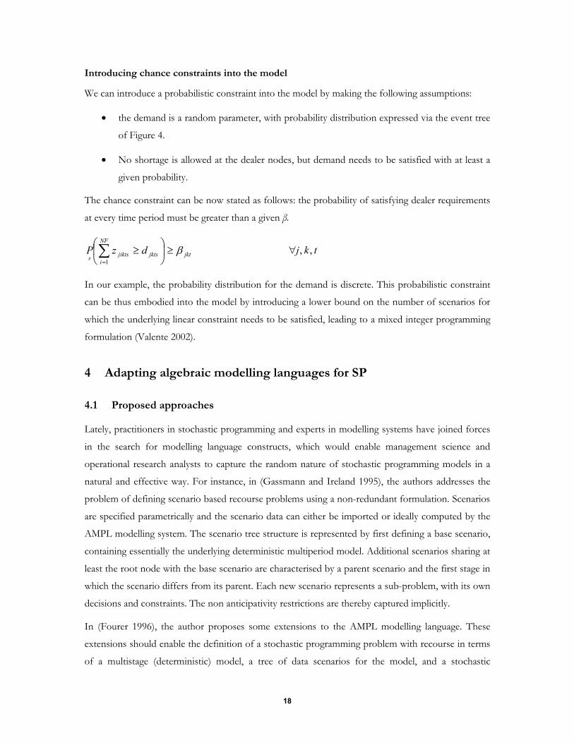
The chance constraint can be now stated as follows: the probability of satisfying dealer requirements

at every time period must be greater than a given β.

jkt

NF

ijktsjiktssdzP

1

tkj ,,

In our example, the probability distribution for the demand is discrete. This probabilistic constraint

can be thus embodied into the model by introducing a lower bound on the number of scenarios for

which the underlying linear constraint needs to be satisfied, leading to a mixed integer programming

formulation (Valente 2002).

4 Adapting algebraic modelling languages for SP

4.1 Proposed approaches

Lately, practitioners in stochastic programming and experts in modelling systems have joined forces

in the search for modelling language constructs, which would enable management science and

operational research analysts to capture the random nature of stochastic programming models in a

natural and effective way. For instance, in (Gassmann and Ireland 1995), the authors addresses the

problem of defining scenario based recourse problems using a non-redundant formulation. Scenarios

are specified parametrically and the scenario data can either be imported or ideally computed by the

AMPL modelling system. The scenario tree structure is represented by first defining a base scenario,

containing essentially the underlying deterministic multiperiod model. Additional scenarios sharing at

least the root node with the base scenario are characterised by a parent scenario and the first stage in

which the scenario differs from its parent. Each new scenario represents a sub-problem, with its own

decisions and constraints. The non anticipativity restrictions are thereby captured implicitly.

In (Fourer 1996), the author proposes some extensions to the AMPL modelling language. These

extensions should enable the definition of a stochastic programming problem with recourse in terms

of a multistage (deterministic) model, a tree of data scenarios for the model, and a stochastic

18

framework to specify the stages and optionally the scenarios and objective. New language constructs

such as scenario and stochastic are introduced to enable the definition of a scenario as a collection of

data and to declare the partition of an underlying time horizon into stages. Scenarios can be solved

individually or as a recourse problem, provided that an appropriate expected value objective is

defined. The authors also hint at the possibility of using a new keyword, namely random, to assign a

probability distribution to given parameters, thus enabling the definition of distribution-based

stochastic programming models.

In (Gassmann and Ireland 1996), the authors also propose extension to the AMPL modelling

language, mainly for the definition of probability distributions of the random parameters. Again, a

language construct random is introduced in distribution-based recourse problems to identify the

random parameters and the variables which depend on these. The same keyword is used in chance

constraint problems, along with the keywords prob and jointprob which are used to declare individual

and joint chance (probabilistic) constraints respectively. Scenario-based recourse problems are dealt

with as in the aforementioned work by the same authors (Gassmann and Ireland 1995). A special set,

called timeset, is defined in all multistage recourse problems and identifies the problem’s stages. An

expectation operator is also proposed to express the expected value of random parameters in

distribution-based models. Finally, the authors propose a number of keywords to indicate specific

probability distributions such as discrete, normal and uniform.

In (Entriken 2001), two additional syntactical items for modelling languages are presented, namely a

random construct for the definition of random parameters, and a relational operator which indicates

precedence between random events. The main idea behind this approach is the fact that stochastic

programming models may be seen as control theory problems, where the random events are assumed

to be input to the system along with the control variables, so that at a given t, only the past outcomes

are known, together with the distribution of the future random parameters. The author uses the

syntax of the AMPL language to declare the underlying linear program, and proposes some new

constructs for the uncertainty. Random parameters are declared using a random qualifier, and are

assumed indexed over the set of outcomes. The importance of the time sequencing of decisions and

events is highlighted and more assumptions (time conventions) are introduced to ensure the correct

order. Also, the relational operators |> and <| are proposed, which provide partial ordering of the

outcomes of the random parameters.

An alternative and innovative approach to modelling stochastic linear programming problems is

presented in (Buchanan, McKinnon et al. 2001). In the paper, the authors define a language called

sMAGIC, which enables the recursive definition of models which contain other (sub) models.

Recursive definition is typical of Dynamic Programming and enables the preservation of the

19

underlying Markov structure, which also characterises many multistage stochastic programming

models. The event tree for models with a Markov structure is compactly represented via a special

direct acyclic graph, which the authors call Model Link Graph (MLG). The nodes of the MLG represent

model or sub-model instances, and arcs connect each model with its nested sub-models. Other work

on extending algebraic modelling languages to support the formulation of stochastic programming

problems include (Gay 2001), (Lopes and Fourer 2003).

4.2 Analysis of modelling issues

Our illustrative example introduced in section 3 highlights the difficulties of using existing algebraic

modelling languages to formulate SP. This is mainly due to the lack of constructs for the definition of

the randomness of the model coefficients and the scenario tree structure. A stochastic programming

model can be considered as a linear programming model extended and refined by the introduction of

uncertainty (see Figure 7). More precisely, the underlying LP optimisation model is extended by

taking into account the probability distribution of the model’s random parameters. Such distributions

are provided by the models of randomness used in scenario generators, which are specific to the

particular optimisation problems under investigation.

STOCHASTIC PROGRAMMING

MODELLING

Modell ing distribution of random parameters

Optimum Allocation Modell ing

- Scenario Analysis - Expected Value - Two Stage RP - Multistage RP - Chance Constrained Problems - Others

Figure 7. The combined paradigm

In general, different categories of stochastic programming problems require different language

features to express the random nature of the problem. We call stochastic framework the information

represented by these constructs.

20

Scenario based recourse problems

The first requirement for the formulation of a stochastic programming problem using algebraic

modelling languages is the declaration of the random parameters. In scenario based recourse

problems, the realisations of such parameters are explicitly given in the form of a scenario tree. Each

scenario is also associated with a corresponding weight (or probability). In turn, the scenario tree

structure is declared in terms of stages. The stages identify the sequence of decisions in the dynamics

of the underlying core model. If the temporal dimension is introduced into the model using a specific

time set, the stages can be declared as subsets of this set. To summarise, the stochastic framework for

scenario based recourse problems requires constructs for the definition following entities:

Entities Language Requirements

stages information assignment of variables and constraints to stages.

scenarios information scenarios set

tree structure

scenario probabilities

random parameters declaration of the random parameters in terms of the scenario

set.

Table 1. Requirements for scenario based recourse problems

Modelling distribution based recourse problems

A number of researchers have proposed extensions to algebraic languages for the formulation of

such class of problems (Fourer 1996; Gassmann and Ireland 1996; Fourer 2001; Gay 2001).

In this work, we focus on the class of scenario-based recourse problems and only outline the

requirements for distribution-based models. Distribution based recourse problems rely on the

declaration of probability distributions for the random parameters. This can be discrete or

continuous. If all random parameters are characterised by discrete distributions, the scenario tree is

implied by the joint realisations of the random parameters. If one or more distributions are

continuous, then there are infinite possible outcomes for the random parameters and the tree

structure must be sampled from the joint distributions. The stochastic framework for distribution

based problems requires constructs for the definition of:

Entities Language Requirements

stages information assignment of variables and constraints to stages.

random parameters declaration of the probability distributions associated with the

d

21

random parameters.

Table 2. Requirements for distribution based recourse problems

Modelling chance constraints

Chance constraints can be added to scenario-based problem or distribution based problems. For

chance constrained models the stochastic framework should identify:

Entities Language Requirements

individual chance constraints

declaration of the individual chance constraints with related

reliability level.

joint chance constraints

declaration of the joint chance constraints with relating

reliability level

random parameters if distribution-based, declaration of the probability distributions

associated with the random parameters

if scenario-based, declaration of the random parameters in

terms of scenarios

Table 3. Requirements for chance constrained problems

4.3 Overview of our approach

Ideally, a modelling language for stochastic programming problems should include a set of constructs

which allow the modeller to capture the effects introduced by the uncertainty on the underlying

model structure. We present a generic approach of expanding AMLs based on the concepts of

underlying deterministic model and stochastic framework. The underlying deterministic model is formulated

using the standard constructs provided by algebraic modelling languages. Using a set of new

constructs, the modeller then declares the stochastic framework, which links the underlying

deterministic model with the model of randomness. More specifically, the underlying deterministic

model represents a family of independent (wait and see) models, while the stochastic framework

imposes the non anticipativity implied by the structure of the scenario tree. The resulting model is

the formulation of the stochastic programming recourse problem. Chance constraints can also be

introduced using specific constructs.

The underlying deterministic

In a typical stochastic programming problem, it is always possible to identify an underlying

deterministic model (also called the core model). The underlying deterministic model captures the

22

logical structure of the problem as well as the dynamical relations within decision variables, their

bounds and the objective function.

In our approach, we construct the core model in such a way that this is parametric in the dimension

of scenarios. All variables and constraints are indexed over the scenarios (which are the element of a

special set declared in the stochastic framework), and the objective function is the expected value

over all scenarios of the individual objectives. As previously mentioned, this formulation is equivalent

to a family of wait and see models.

Declaration of the stochastic framework

As we have shown in section 4.2, the stochastic framework depends on the type of stochastic

programming model which is being developed. For instance, scenario based recourse problems

require the explicit declaration of the scenario tree structure, while in a chance constrained problem

the framework includes information on one or more probabilistic constraints. Finally, in a

distribution based recourse problem, the AML should provide a set of constructs for the definition

of probability distributions.

Time index

Stages

aggregations

Scenario tree structure

Scenario index

Random

parameters

Scenario

probabilities

Probabilistic constraints

Indices

Objectives

Constraints

Variables

Parameters

Standard AML constructs sufficient for the definition of the core models

Extensions for SP modelling

Figure 8. Extended language constructs

Figure 8 shows how the basic constructs of a modelling language for linear programming are

extended to capture the stochastic framework. The definition of the new constructs is adapted to be

consistent with the grammar of the underlying modelling language. We have successfully applied this

approach to the AMPL language, although the same ideas can be adapted to virtually any other AML

(see for instance (Valente, Mitra et al. 2001) for an application to MPL). The syntax of the extended

language constructs for AMPL (which we call SAMPL) is defined in the next section.

23

4.4 SAMPL language extensions

Taking into account the requirements expressed in the section 4.2, we have designed a set of new

constructs for the AMPL language, which support the declaration of the stochastic framework

information.

Stages

The assignment of variables and constraints to the different stages of the dynamic recourse model is

essential in the definition of stochastic programming recourse models.

A generic approach considers the existence of a time set, which is used as an index for all variables of

the model. Then a partition of such time set can be given, so that several time periods (and the

variables which relate to these time periods) can be grouped into a single stage. We have

implemented this approach in extending the MPL modelling language (Valente, Mitra et al. 2001).

However, the fact that modellers are forced to introduce the time dimension for all variables could

result in a very unnatural modelling. This is particularly true in two stage models, where the first stage

and second stage decisions are usually defined using different vectors, and hence already

“distinguished” from one another.

An alternative and more flexible approach is viable using modelling languages (such as AMPL),

which enable the definition of suffixes. A suffix can be considered as a generic property of a variable

or constraint, and can be used for our purpose to declare the stage which a variable belongs to. The

stage of the constraints is determined by the stage of the variables which appear in it. The highest

stage of any of such variables is the stage of the constraint.

The syntax for the assignment of a stage number to a variable is very similar to that of AMPL for

other suffixes, but makes use of a predefined suffix called stage:

suffix stage IN; let indexingopt name.stage := expr;

Alternatively, AMPL enables the suffix to be given in the variable declarations:

var name aliasopt indexingopt attributesopt, suffix stage expr;

In the example distribution model, variables are indexed over a time set. The staging for the two-

stage problem can be expressed as:

suffix stage IN; var xProd,Fact,t in Time,Scen >=0, suffix stage if t=1 then 1 else 2; var yProd,Fact,t in Time,Scen >=0, suffix stage if t=1 then 1 else 2; var wProd,Deal,Time, Scen >=0, suffix stage if t=1 then 1 else 2; var zProd,Fact,Deal,Time, Scen >=0, suffix stage if t=1 then 1 else 2;

24

Figure 9 shows the aggregation of time periods into stages for the two-stage distribution model.

3 4 2 1

stage 1 stage 2

Figure 9. Two-stage aggregation.

In the multistage model, the stage of a variable is simply given by the time period which the variable

belongs to:

suffix stage IN; var xProd,Fact,t in Time,Scen >=0, suffix stage t; var yProd,Fact,t in Time,Scen >=0, suffix stage t; var wProd,Deal,Time, Scen >=0, suffix stage t; var zProd,Fact,Deal,Time, Scen >=0, suffix stage t;

Figure 10 shows the aggregation of time periods into stages for the multistage distribution model.

3 4 2 1

stage 1 stage 2 stage 3 stage 4

Figure 10. Multistage aggregation.

Scenarios information

Information about the scenario tree which characterises scenario-based recourse problems is

provided by the modeller via a set of new keyword, which describe below:

Scenario set In scenario-based recourse problems, the uncertainty represented by the random parameters

introduces a new dimension, identified by the scenario set. This set needs to be explicitly identified,

because the random parameters are indexed over it. The syntax used for the declaration of the

scenario set follows the syntax of AMPL for sets, but uses scenarioset instead of set in the declaration:

scenarioset name aliasopt indexingopt attribsopt ;

Considering the example model given in section 3, the scenario set is declared as:

param NS:=8; … #stochastic framework … scenarioset Sc:=1..NS; …

25

Scenarios probabilities The probability distribution of the scenarios is declared using a special parameter vector, whose

elements are the weights of the individual scenarios. The parameter is therefore indexed over the

scenario set. The syntax used is similar to the AMPL syntax for the declaration of the other

parameters, but uses the probability keyword instead of (or before) the param keyword. The syntax is

the following:

probability paramopt name aliasopt indexingopt attributesopt ;

Example:

… scenarioset Sc:= 1..NS; probability param PrSc:=1/card(Sc); …

Scenario Tree The tree keyword is used to define the scenario tree structure. In general, this structure can be

considered as a set of pairs (scenario,stage), which identify the branches (and therefore the nodes) of

the tree. Our language constructs enable the modeller to specify “well structured” trees in a concise

way. The syntax is as follows:

tree name:=opt tree_declaration ;

where tree_declaration is one of:

bundle_list | tlist | nwayn| multibranchn1, n2,...,nST| binary | twostage nsopt ;

bundles A bundle list is defined as:

bundle_list : bundlesBundle-1, Bundle-2,.. Bundle-n ;

where:

Bundle-x: (stagex,scenx);

A bundle is associated to each node of the tree and consists of the stage in which the node lies, and a

scenario number defined as the minimum of the ordinal values associated with the scenarios which

pass through the same node (King 1994). Considering the tree structure of Figure 11, its bundles

representation is formulated as:

… tree Tree:= thebundles

26

(1,1), (2,1),(2,4),(2,6), (3,1),(3,4),(3,6),(3,7), (4,1),(4,2),(4,3),(4,4),(4,5),(4,6),(4,7)(4,8),(4,9) ;

3 4 5 6

8

2

9

7

1 1 2 3 4

Figure 11. Example of asymmetric tree.

tlist An very compact representation of asymmetric trees can be obtained if the following assumption

holds:

Scenarios are indexed in an order that ensures complete separation of all nested sub-trees (i.e. the scenario paths

never cross one another)

In this case, a scenario tree can be represented as a list of S elements (tlist) whose values are the stage

numbers where a scenario branches from its father scenario. A tlist can thus be constructed by

considering the column number associated to the leftmost element of each row of the tree matrix.

The syntax for the tlist tree is the following:

tlist: tlistn1, n2,.. nS;

As an example, the tlist representing the scenario tree of Figure 11 is set out below:

… tree theTree:= tlist 1,4,4,2,4,2,3,4,4; …

In many applications, however, the scenario tree is characterised by a "standard" structure: the

following keywords simplify the definition of such trees:

nwayn; Defines a tree where a constant number n of branches occur at each stage σ=1..ST-1, where ST is the

number of stages in the model. The total number of scenarios S of the problem is hence determined

by the following expression:

1

STnS

27

This must be consistent with the cardinality of the scenario set defined using the scenarioset keyword.

multibranchn1, n2,...,nST; Defines a tree where at each stage σ=1..ST-1 is associated a number of branches nσ. The NWAY tree

is a particular case of the MULTIBRANCH tree, where nσ is constant. The total number of scenarios

S of the problem is therefore:

1

1

ST

nS

binary A binary tree is such that at each time stage, two possible outcomes of the random data can be

observed. The total number of scenarios S of the problem has to satisfy the following equality:

12

STS

twostage nSOpt If the model is a two-stage recourse model, then the tree structure can be declared using the twostage

keyword. This is equivalent to define an nwayns tree, where ns is the number of scenarios for the

model.

Random parameters

The random parameters of the model have to be identified and distinguished from the deterministic

model data. If the model is scenario based, every parameter of the model which is random, needs to

be explicitly identified as such. Also, the scenario dimension must be added to the indexing list of the

parameter.

random param name indexing attributesopt;

In our deterministic example of section 3.1, the demand parameter is defined as:

… param dProd,Deal,Time,Scen >=0; #demand …

Using the random keyword, we explicitly redefine the parameter as a random variable:

scenarioset Sc:=1..NS; … random param dProd,Deal,Time,Scen >=0; #demand …

The particular nature of the multistage stochastic programs with recourse introduces the choice

between diverse forms of presenting the data values for the random parameters. These forms can be

either compact or expanded. The compact form assumes that the scenario data can present itself in the

form of a 2-dimensional matrix (tree matrix) where only some of the entries exist. The matrix forms

28

a grid where the columns represent time periods and the rows represent scenarios. The conditions

under which such a matrix, partially entered, can represent a tree may be stated as follows:

1. Entry (1,1) must exist

2. Entries (T,s) exist for all scenarios s=1..S, where T is the number of time periods and S the

number of scenarios.

3. If entry (t,s) exists for some t<T, then also does entry (t+1,s).

Each entry (t,s) of the matrix represents the realisation of the random parameter at time period t

under scenario s. An entry can consist of a single value or a vector of values if the random parameter

is indexed over sets other than the time set and the scenario set.

For instance, let us consider a 3 time period horizon and random parameter p, which takes the

(known) value 10 in the first time period. Let us consider that 2 realisation of the random parameter

can be observed at each time period t=2..4, as in figure Figure 12:

p(t)

p(t+1)=p(t)+50%

p(t+1)=p(t)-50%

Figure 12. Simple event tree rule.

This rule defines a simple scenario generator, whereby a binary tree can be constructed, as in figure

Figure 13.

10

15

5 7.5

7.5

2.5

22.5

1

2

3

4

Figure 13. Binary scenario tree.

The (sparse) matrix representing the data for this scenario tree is shown in Table 4:

t=1 t=2 t=3

10 5 2.5 s=1

7.5 s=2

29

15 7.5 s=3

22.5 s=4

Table 4.Compact scenario data.

Such matrix can be represented in SAMPL in a row-wise fashion as:

#model file scenarioset scen = 1..4; random param demt,scen; … #data file random param dem:= 1 1 10 2 1 5 2 3 15 3 1 2.5 3 2 7.5 3 3 7.5 3 4 22.5;

Although the data format here illustrated avoids any possible redundancy, it often happens that the

scenario data are provided in what we call expanded form. This can be thought as the tree matrix

above, where all entries are given. The expanded matrix relative to the example previously

investigated is shown in Table 5:

t=1 t=2 t=3

10 5 2.5 s=1

10 5 7.5 s=2

10 15 7.5 s=3

10 15 22.5 s=4

Table 5. Expanded scenario data.

The data for the random parameter demT,S are expressed in tabular form as follows:

#data file random param dem (tr):= 1 2 3 1 10 5 2.5 2 10 5 7.5 3 10 15 7.5 4 10 15 22.5;

Chance constraints

Probabilistic (or chance) constraints are characterised by randomness in some of the coefficients and

by a level β which indicates the probability of satisfying the constraint. Chance constraints are defined

using the following syntax:

chance indexingopt constraint_name relop expression;

30

where relop is one of ≤ , ≥. Consider the following deterministic constraint vector definition in

AMPL:

satisfy_demandj in Prod, k in Deal, t in Timem, s in Scen: sumi in Fact z[j,i,k,t,s] >=d[j,k,t,s];

Assuming that d[j,k,t,s] is a random parameter with realisations given in the form of scenarios, the

constraint can be transformed into a probabilistic one as in the following example:

s cenarioset Sc:=1..NS;

random param dProd,Deal,Time, Scen >=0 #demand param beta := 0.9; satisfy_demandj in Prod, k in Deal, t in Time, s in Scen: sumi in Fact z[j,i,k,t,s] =d[j,k,t,s]; > chancej in Prod, k in Deal, t in Time,s in Scen satisfy_demand[j,k,t,s]>=beta;

The chance statement indicates that each row of the constraint vector satisfy_demand has to be satisfied

with probability greater than 0.9.

4.5 Implementation of the illustrative examples in SAMPL

In this section, we combine the AMPL standard constructs with the proposed SAMPL extension in

order to formulate the illustrative example of section 3 in its two-stage, multistage and chance

constrained versions. More specifically, we first formulate the underlying deterministic model (Wait

and See) in AMPL, and then add the stochastic information using the SAMPL constructs.

The underlying deterministic model

The underlying deterministic model associated with the problem illustrated in section 3 can be

formulated in AMPL as follows:

#distribution model clo2s.mod param NT; param NK; param NP; param NF; param NS; set Fact:= 1..NF; set Prod:= 1..NP; set Deal:= 1..NK; set Time:= 1..NT; set Scen:= 1..NS; param q Prod, Fact ; #unit prod cost param c Fact,Deal; #unit transportation cost param v Prod, Fact ; #prod capacity param a Prod, Fact ; #inventory cost param lProd,Fact; #Initial inventory param nProd,Fact; #Inventory capacity p aram pProd,Deal; #Shortage penalty

param dProd,Deal,Time,Scen; #demand param PrScen:=1/card(Scen); #Probability of the scenarios var xProd,Fact,Time,Scen >=0; #production

31

var yProd,Fact,Time, Scen >=0; #inventory var zProd,Fact,Deal,Time, Scen >=0; #shipment var wProd,Deal,Time, Scen >=0; #shortage minimize cost: sum(s in Scen Pr[s]* (sumj in Prod, i in Fact, t in Time q[j,i]*x[j,i,t] + sumj in Prod, i in Fact, k in Deal, t in Time c[i,k]*z[j,i,k,t] + sumj in Prod, i in Fact, t in Time v[j,i]*y[j,i,t] + sumj in Prod, k in Deal, t in Time p[j,k]*w[j,k,t]); subject to satisfy_demandj in Prod, k in Deal, t in Time, s in Scen: sumi in Fact z[j,i,k,t,s] + w[j,k,t,s]=d[j,k,t,s]; inv_balance_initj in Prod, i in Fact, s in Scen : x[j,i,1]+l[j,i]=y[j,i,1]+sumk in Deal z[j,i,k,1,s]; inv_balancej in Prod, i in Fact, t in 2..NT, s in Scen : x[j,i,t,s]+l[j,i]=y[j,i,t,s]+sumk in Deal z[j,i,k,t,s]; inv_capacityj in Prod, i in Fact, t in Time, s in Scen : y[j,i,t,s]<=n[j,i]; prod_capacityj in Prod, i in Fact, t in Time, s in Scen : x[j,i,t,s]<=a[j,i];

The two stage recourse model

To illustrate the use of the new constructs for stochastic programming described in the previous

section, we modify the above deterministic model as follows:

scenarioset Scen:= 1..NS; #declares Scen as the “special” scenario set; tree theTree:= twostageNS; #declares a two stage tree with NS scenarios random param dProd,Deal,Time,Scen; #declares demand as random parameter probability param PrScen:=1/card(Scen); #declares the probability of the scenarios suffix stage IN; #assigns variables to stages var xProd,Fact,Time,Scen >=0, suffix stage if t=1 then 1 else 2; var yProd,Fact,Time,Scen >=0, suffix stage if t=1 then 1 else 2; var zProd,Fact,Deal,Time,Scen >=0, suffix stage if t=1 then 1 else 2; var wProd,Deal,Time,Scen >=0, suffix stage if t=1 then 1 else 2;

The set Scen is defined using the scenarioset keyword, which identifies it as a special set. The tree

keyword is used to define the structure of the scenario tree as a two-stage (fan) tree.

The parameter d is declared using the random param keyword, while the probability vector Pr is

redefined as probability param. Finally, the variables are partitioned into different stages by adding of

the suffix stage to their definition.

From two stage to multi stage

Transforming the two-stage model to a multistage formulation for the same problem is very easily

achieved using the SAMPL constructs. It is necessary to disaggregate the stages, and assign variables

of different time periods to distinct stages. The tree structure of the model is also revised to that of

the multistage tree of Figure 6. The resulting stochastic framework is set out as follows:

32

scenarioset Scen:= #declares Scen as the “special” scenario set; 1..NS; tree theTree:= nway5; #declares tree with 5 branches at each stage random param dProd,Deal,Time,Scen; #declares demand as a random parameter probability param PrScen:=1/card(Scen); #declares the probability of the scenarios suffix stage IN; #assigns variables to stages var xProd,Fact,Time,Scen >=0, suffix stage t; var yProd,Fact,Time,Scen >=0, suffix stage t; var zProd,Fact,Deal,Time,Scen >=0, suffix stage t; var wProd,Deal,Time,Scen >=0, suffix stage t;

Chance Constrained Problem in SAMPL

The chance-constrained version of the same problem is also formulated using the extended language

constructs. The underlying deterministic model is first revised in the following way:

1. Change the satisfy_demand constraint to allow for shortages. (This means that variable w is not

required any longer, and that the shortage cost is also removed from the objective function)

2. Define a reliability parameter which represents β of equation (17).

A few additional SAMPL statements are added, including the declaration of the constraints named

satisfy_demand as chance in the stochastic framework. The resulting model is set out below.

#distribution model cloccp.mod param NT; param NK; param NP; param NF; param NS; set Fact:= 1..NF; set Prod:= 1..NP; set Deal:= 1..NK; set Time:= 1..NT; scenarioset Scen:=1..NS; param reliabilityProd,Deal,Time; # beta level for the chance constraint param qProd,Fact >=0; #unit prod cost param cFact,Deal >=0; #unit transportation cost param pProd,Deal >=0; #Shortage penalty param vProd,Fact >=0; #prod capacity param aProd,Fact >=0; #inventory cost param lProd,Fact >=0; #Initial inventory param nProd,Fact >=0; #Inventory capacity probability param PrScen:=1/card(Scen); #probability vector random param dProd,Deal,Time,Scen; #demand var xProd,Fact,Time, Scen >=0; #production var yProd,Fact,Time, Scen >=0; #inventory var zProd,Fact,Deal,Time, Scen >=0; #shipment minimize cost: sums in Scen Pr[s]*( sumj in Prod, i in Fact, t in Time q[j,i]*x[j,i,t,s] + sumj in Prod, i in Fact, k in Deal, t in Time c[i,k]*z[j,i,k,t,s] + sumj in Prod, i in Fact, t in Time v[j,i]*y[j,i,t,s]); subject to … satisfy_demandj in Prod, k in Deal, t in Time,s in Scen: sumi in Fact z[j,i,k,t,s] >=d[j,k,t,s];

33

inv_balance_initj in Prod, i in Fact, s in Scen : x[j,i,1,s]+l[j,i]=y[j,i,1,s]+sumk in Deal z[j,i,k,1,s]; inv_balancej in Prod, i in Fact, t in 2..NT, s in Scen : x[j,i,t,s]+l[j,i]=y[j,i,t,s]+sumk in Deal z[j,i,k,t,s]; inv_capacityj in Prod, i in Fact, t in Time, s in Scen : y[j,i,t,s]<=n[j,i]; prod_capacityj in Prod, i in Fact, t in Time, s in Scen : x[j,i,t,s]<=a[j,i]; # definition of the constraint satisfy_demand as chance constraint chancej in Prod, k in Deal, t in Time, s in Scen satisfy_demand[j,k,t,s]>=reliability[j,k,t];

5 Implementation of the language extensions

Algebraic modelling languages are supported by modelling systems, which provide connectivity to data

sources and solvers. The developers of algebraic modelling languages do not seem to be yet ready to

undertake the laborious effort needed to extend their systems to include stochastic programming

constructs. Some key aspects need to be taken into account:

The inadequacies of existing matrix representation formats for SP problems, used to connect

solvers to the modelling systems.

The problem of linking modelling systems with scenario generators.

The risk of introducing languages features which are not yet fully accepted by the OR

community, nor by the developers themselves.

In this section, we address the first two issues and briefly introduce our SPInE system, which

implements the language extensions presented in this paper and is readily connected with SP solvers

and scenario generators.

5.1 Interfacing modelling systems and solvers

The main problem associated with the interfacing of modelling system and specialised SP solvers is

the representation and communication of the SP model instances.

Representation of SP model instances.

The SMPS format as introduced in (Birge, Dempster et al. 1988) enables the compact representation

of large scale stochastic programming problems, including scenario based recourse problems.

However, in (Gassmann and Schweitzer 2001) the authors illustrate a number of shortcomings

associated with this standard. The authors propose an extended SMPS format with added

34

representational power which overcomes most of the problems associated with the original standard.

In this research, however, other types of problems have been identified, which cannot be directly

represented using the SMPS standard, nor its extended version.

Recourse problems without first stage constraints.

Consider the following simple problem, which is a variant of the newsboy problem:

The newsboy needs to decide, every day, what is the optimal number of newspaper x to buy in order

to maximize the profits. The demand D is not known with certainty. A set of scenarios S for the

demand is given. The outcomes of the demand for each scenario s in S are defined as Ds and the

associated probability is Ps. Each copy of the newspaper is characterized by a unit selling price R and

a unit purchase cost C. Unsold copies ys+ represent a loss for the newsboy. The eventual shortfall of

copies is indicated with ys- and is characterised by a penalty term in the objective function. Shortfall

and excess are only revealed once the demand is known, hence x is a first stage variable, while ys+ and ys-

are second stage variables. The algebraic formulation of the two-stage model can be stated as follows:

Ss ..

)()(max

sss

Ssss

Ssss

Dyyxts

yPRyPCRxCRprofit

(18)

where the objective is to maximise the profit, expressed as the profit of selling all the newspaper

purchased, minus the expected value of the (false) profit generated by the unsold copies and the

expected value of the shortfall penalty. The ordered matrix of this problem, for |S|=3 is the

following:

x

1y

1y

2y

2y

3y

3y

R-C P1(R-C) P1R P2(R-C) P2R P3(R-C) P3R

1 1 -1 D1

1 1 -1 D2

1 1 -1 D3

This degenerate type of models is characterised by two difficulties, namely the fact that the first stage

constraints are missing and that the first stage problem is unbounded. The first feature precludes the

possibility of representing the model using the SMPS format. Indeed, the time file of the SMPS

requires the specification of the top-left element of the block of non-zeroes identified by the

35

variables and constraints which belong to each stage. In this case, the block relating to the first stage

is empty, hence SMPS cannot be adopted.

Also, if the first stage problem is unbounded, solution algorithms based on Benders’ decomposition

may fail. In general, these algorithms try to solve a master problem associated with the first stage in

order to obtain a feasible first stage solution, which is then refined by solving sequences of

subproblems (associated with second stage) which are parametric in the first stage decision. The

solution of the subproblems leads to cuts which are added to the master problem until the optimum

solution is found. If the master is unbounded, the algorithm may fail even if the problem as a whole

is feasible. An approach to deal with this problem is to create some artificial bounds on the first stage

variables during the very first iteration of the decomposition algorithm. This may provide a feasible

starting decision for the subsequent solution of the subproblems.

Global constraints

The term “global constraint” is used in the context of this research to identify a class of constraints

which may be required in some scenario based stochastic programming problems. A global

constraint is a constraint which involves decision variables associated with different nodes of the

scenario tree. Consider for instance the following two-stage recourse problem:

kyrphytxu

baxts

yfpcx

Sssss

ssss

Sssss

Ss

..

min

(19)

The associated matrix for |S|=3 is the following:

x 1y 2y 3y

c p1f1 p2f2 p3f3

a b

u1 t1 h1

u2 t2 h2

u3 t3 h3

p1r1 p2r2 p3r3 k

36

The last row links variables belonging to three different scenarios. One of the underlying

assumptions of SMPS is that the blocks of the matrix which relate to different scenarios need to be

completely separable, therefore these types of problems cannot be represented using the SMPS

format. Global constraints are generally used to introduce restrictions on the expected value of some

function of the decision variables. Typical examples of such functions are risk measures such as the

Expected Downside Risk or the Conditional Value at Risk (CVaR).

A modelling system which supports stochastic programming modelling should therefore take into

account the issues related to the representation of the model instances. In the specific case of global

constraints, the modelling system should be able to detect such expressions and move the constraint

into the objective function with as a penalty term.

New directions: XML

The limitations of the SMPS format in terms of representational power have become apparent over

the years, and some extensions have been proposed (Gassmann and Schweitzer 2001). Recently,

researchers have expressed significant requirements for an enhanced standard, specifically for the

purpose of communicating mathematical programs. A new approach, which takes into consideration

contemporary technical assumptions, is based on eXtended Mark-up Language (XML). The wealth of

functionality and software available for exploiting XML is an important factor in the acceptance of

an XML based mathematical programming standard. There are currently at least three XML

vocabularies proposed for this role: FML (Fourer, Lopes et al. 2003), OptML (Kristjansson 2001)

and SNOML (Lopez and Fourer 2001). Both support linear and non-linear optimisation models, but

in addition, SNOML is also able to capture stochastic programming models with recourse, chance-

constrained models, and also constraint logic programming models.

At this stage, OptML and SNOML are not fully designed nor accepted by the research community;

however, they seem to be the most promising approaches towards a new standard for the

representation and communication of mathematical programming problems, including stochastic

programming models.

5.2 Communicating with scenario generators

Linking scenario generators with modelling systems

The creation of the scenario tree used in multistage stochastic programming is usually carried out by

specialised applications called scenario generators. While the algebraic optimisation model captures the

logic of the application’s domain, the scenario generators are special purpose applications developed

to capture the randomness properties of the application’s domain. Typically, a consumer product

37

supply chain model and an energy distribution model both require scenarios of forecast demand, but

the factors which influence the demands and the forecasting models may be very different. Again in

finance applications the asset prices under consideration may be generated using different models of

credit risk (Jobst 2002), interest rate risk or other considerations. In designing an SP modelling

system, one goal is therefore to develop an appropriate parameter passing interface which enables the

connection of diverse special purpose scenario generators (which capture valuable domain

knowledge) to the modelling system

A scenario generator φ captures in a procedural form a domain-specific model of randomness. In

particular it uses historical information, an event tree structure and some other specification

parameters to forecast a set of scenarios. The main groups of parameters can thus be separated as:

H : History,

τ: : Event Tree,

θ : Remaining Parameters.

The set of scenarios Ξ is then seen as the collection of scenarios which are output by the generation

procedure:

),,( H (20)

The data associated with the set of scenarios Ξ are implicitly structured as the event tree τ. This event

tree is usually specified in terms of a time horizon T and the number of outcomes of the random

parameters per time period. Trees with arbitrary structures are typically defined by specifying the

underlying node structure. The historical data H are often used to determine an underlying

probability distribution for the random parameters. Historical data may also contain the initial values

(that is, the values assumed by the random parameters in the root node of the scenario tree). If the

historical data are not used to determine the probability distributions, the set of remaining parameters

θ may include the type of distribution and estimates of its moments.

The tree structured outcomes of the random parameters τ, induce a similar structure in the

underlying optimum decision making problem, as the variables and constraints are dependent on the

realisations of the random parameters. This is a central question which needs to be addressed when

modelling stochastic programming problems using algebraic modelling languages: the algebraic form

of the SP model requires the specification of the ‘variable and constraint’ tree structure, labelled as τ’.

An extended AML should provide constructs for the specification of τ’ in the SP model. For

consistency, the two trees τ and τ’ need to be congruent. In other words, it has to be ensured that the

38

event tree structure τ used by the special purpose scenario generator is ‘compatible’ with the τ’

specified in the SP model and vice versa (Valente, Mitra et al. 2001). The requirement for scenario

generator parameter passing and tree consistency conditions are illustrated in Figure 14. When a

special purpose scenario generator is connected to the modelling system, the two trees τ and τ’ are

compared for consistency. The scenario generator then creates the set of scenarios and the associated

probabilities p(ω).

Model of randomness

Scenarioset

SP recourse model

(requires tree structure):

’

H

’ H

: Scenario tree structure : SP model tree structure : Model of randomness : Other parameters of : Historical data : Set of scenarios

Consistency condition:

’

Figure 14. Scenario Generation and Tree Consistency

If the scenario generation procedure is kept separated from the modelling system, the consistency of

τ and τ’ can be ensured if the algebraic specification of the model enables the definition of τ’ as a

special model parameter. This is then instantiated using τ, which therefore needs to be explicitly

provided by the scenario generator along with the scenario data Ξ. The modelling system should be

able to use the information in the special parameter τ’ to introduce the structure in the model’s

variables and constraints, either via explicit non-anticipativity constraints, or implicitly by creating the

appropriate variables and constraints for each node of the tree. This approach is consistent with the

modelling process using systems based on declarative algebraic languages: the algebraic model and

the data (deterministic data, scenarios data and the tree structure, in this case) are kept separated.

A desirable aspect of modern algebraic modelling languages is to include procedural features; for

instance, many procedural constructs enable closer coupling with the solvers. The same concept

could be applied to enable a closer coupling of modelling system with external scenario generators.

The tree structure τ’, the historical data H and the remaining parameters θ are defined using the

algebraic modelling language, and the modelling system provides procedural constructs to “call” the

scenario generator passing the parameters. The resulting scenario data is then consistent with τ’ and

can be used to instantiate the stochastic programming model. Unfortunately, these features are not

directly available in modern modelling systems. A major focus of this research is to introduce special

39

purpose language constructs for the definition of scenario based recourse problems and an integrated

system which supports these language constructs. These together enable the seamless integration of

algebraic modelling with scenario generation procedure using the paradigms discussed in this section.

5.3 Integrated environments: SPInE

Our implementation of the SAMPL language processor is the core of the modelling subsystem of

our Stochastic Programming Integrated Environment (SPInE) (Valente, Mitra et al. 2002).

SPInE is divided into four main subsystems, namely Scenario Generation, Modelling, Solver, Results

Analysis and the overarching Control module.

Scenario Generation

SPInE is designed to interface with scenario generators which supply the scenario data in ODBC

databases or text files. An important aspect of the scenario generation interface is to establish the

consistency between the SP model tree τ’ and the data path tree τ underlying the scenario generation

(see Section 5.2).

Modelling subsystem

The modelling subsystem is designed to support the SAMPL language extensions introduced in this

report. Similarly, it supports the SMPL stochastic extensions of the MPL language. A software

module called Stochastic Program Generator (SPG) combines two separate parsers and a matrix

generator. SPG processes together the algebraic models and the scenario data set to create an

instance of the model in either SMPS format or in the Stochastic Intermediate Representation (SIR).

The SPG module makes use of an underlying modelling engine, specifically OptiMax for the support of

SMPL models and a comparable AMPL-based COM object, developed by our research group, for

models prepared in SAMPL. The modelling system interacts directly with the scenario generators for

the stochastic data can connect to database systems or data files which store the deterministic data

relating to the core model of the SP problem.

Solver subsystem

Given a Stochastic Programming problem with recourse, formulated in SAMPL, the FortSP

stochastic solver embedded in SPInE (Poojari, Ellison et al. 2002) provides the solution to three

related classes of models:

Here and Now

Scenario Analysis (Wait and See)

40

Expected Value

For each of these, there is more than one possible solution algorithm. All underlying LPs may be solved

using the Sparse Simplex algorithm (SSX) or the Interior Point Method (IPM). The Here and Now

problem may be solved using Benders Decomposition, Lagrangean Relaxation or via the

Deterministic Equivalent problem. The solver is also able to report the stochastic measures EVPI

and VSS.

Results analysis

A critical phase in the development of stochastic models is the analysis of the solutions. The

integration with database systems enables the exploitation of the Data Manipulation Languages

(DML) which usually accompany the DBMS for the development of customised viewers and

advanced data analysis tools. The SP Reporter (SPR) module of SPInE allows the user to export

solution vectors using standard ODBC or using text files. The volume of the solution results

produced by the stochastic solver can be very large. In fact, each decision variable has an associated

optimal activity and reduced cost, for each stage and for each scenario. The investigator might be

interested only in a subset of the solutions (e.g. the first stage strategic decisions). SPR provides

filtering functionality which is used to transfer only the relevant decision data to the DBMS.

Control Module and Graphical User Interface

Each module in SPInE can be run as an independent application through script files. A control

module including a Graphical User Interface (GUI) has been developed and can be used to

investigate SP problems. The main subsystems of SPInE, namely the SP instances generator SPG,

the stochastic solver FortSP and the solution Reporter SPR have also been wrapped in a dynamic

link library, which enables the rapid development of embedded applications.

6 Conclusions and directions for future research

Modelling and solving stochastic programming problems is a challenging task. Stochastic

programming models can be transformed into deterministic equivalent formulations by discretising

the support of underlying continuous probability distributions. However, it is often impossible to

take advantage of the existing modelling tools and LP/MIP solvers to formulate and process these

models. In this report, we have identified a number of modelling requirements for stochastic

programming. Taking these into account, we have designed an approach to extending algebraic

modelling languages for the formulation of SP models in a natural and concise way and we have

shown how this approach can be applied to the AMPL modelling language with a practical example.

41

The difficulties associated with the modelling of the random parameters for SP problems are

discussed, and some insight is gained into the relations between scenario trees and SP model

structures; thereby the requirements for the seamless integration of scenario generators and

modelling systems are identified. Current algebraic modelling languages are required to capture the

scenario structures of SP models. The problem of representing instances of stochastic programming

models in formats which can be exploited by specialised solution algorithms are also studied.

A number of issues which remain to be addressed have been identified in respect of the process of

modelling, solution and analysis of stochastic programming problems.

The language constructs proposed in this research only address the class of scenario-based stochastic

programming problems, while distribution-based problems also need to be considered. The

definition of the random parameters using probability distributions needs to take into account the

complexity introduced, for instance, in multistage problems. In these models, there might be

dependency of the random variables across stages, which implies the use of conditional probabilities.

The integration of scenario generators requires further investigation. This aspect is strictly connected

with the possibility of defining models of randomness directly in the modelling language. An

alternative would be the introduction of a mechanism (eventually based on new language constructs)

for the control of the scenario generation in algebraic modelling languages which support procedural

statements. A library of standard scenario generators which readily connects to the SPInE system is

under way. This will enable practitioners to truly deploy the system for a complete investigation of

stochastic programming problems, and will also expand the capabilities of the simulation framework.

42

7 References

Birge, J. R., M. A. H. Dempster, H. I. Gassmann, E. Gunn, A. J. King and S. W. Wallace (1988). "A standard input format for multiperiod stochastic linear programs." Mathematical Programming Society Committee on Algorithms Newsletter 17, 1-19. Bisschop, J. J. and M. Roelofs (1999). "AIMMS: The Language Reference." Paragon Decision Technology BV, Haarlem, The Netherlands. Bosetti, V., E. Messina and P. Valente (2002). "Optimisation technologies and environmental applications." submitted to the IMA Journal of Management Mathematics. Brooke, A., D. A. Kendrick, A. Meeraus and R. Raman (1998). "GAMS : a user's guide,Release 2.50." Buchanan, C. S., K. I. M. McKinnon and G. K. Skondras (2001). "The Recursive Definition of Stochastic Linear Programming Problems within an Algebraic Modeling Language." Annals of Operations Research 104(1), 15-32. Charnes, A. and W. W. Cooper (1959). "Chance-constrained programming." Management Science 5, 73-79. Entriken, R. (2001). "Language Constructs for Modeling Stochastic Linear Programs." Annals of Operations Research 104(1), 49-66. Eppen, G. D., R. K. Martin and L. Schrage (1989). "A Scenario Approach to Capacity Planning." Operations Research 37(4), 517-527. Escudero, L. F., E. Galindo, G. Garcia, E. Gomez and V. Sabau (1999). "Schumann, a modeling framework for supply chain management under uncertainty." European Journal of Operational Research 119(1), 14-34. Fourer, R. (1996). "Proposed new AMPL features - stochastic programming extensions." www.ampl.com/cm/cs/what/ampl/NEW/FUTURE/stoch.html. Fourer, R. (2001). "Model-level directives for generating alternative formulations of stochastic programs." IX International Conference on Stochastic Programming,, Berlin, Germany. Fourer, R., D. M. Gay and B. W. Kernighan (1993). "AMPL : a modeling language for mathematical programming." Danvers Mass Boyd Fraser Pub. Co,. Fourer, R., L. Lopes and K. Martin (2003). "A W3C XML schema for linear programming." Northwestern University and The University of Chicago, (work in progress). Gassmann, H. I. and A. M. Ireland (1995). "Scenario formulation in an algebraic modelling language." Annals of Operations Research 59, 45-76. Gassmann, H. I. and A. M. Ireland (1996). "On the formulation of stochastic linear programs using algebraic modelling languages." Annals of Operations Research 64, 83-112. Gassmann, H. I. and E. Schweitzer (2001). "A comprehensive input format for stochastic linear programs." Annals of Operations Research 104(1), 89-125.

43

44

Gay, D. M. (2001). "Random parameters - a step toward conveniently expressing some stochastic programming problems." IX International Conference on Stochastic Programming, Berlin, Germany. Jobst, N. (2002). On credit risk modelling, simulation, optimisation. PhD thesis, Department of Mathematical Sciences. Uxbridge, UK, Brunel University. King, A. J. (1994). "SP/OSL Version 1.0 Stochastic Programming Interface Library: User' s Guide, Research Report RC 19757 (87525) 9/26/94 Mathematics." T.J Watson Research Center, Yorktown Heights, NY. Kristjansson (2001). "How New Technologies such as XML and SOAP allow OR to provide Web-based Services." INFORMS Roundtable Savannah, Georgia. Lopes, L. and R. Fourer (2003). "A modeling language for stochastic programming." ISMP 2003, Copenhagen, Denmark. Lopez, L. and R. Fourer (2001). "An XML-Based Format for Sharing Mathematical Programs." INFORMS international conference on Miami, November 2001. Lucas, C., E. Messina and G. Mitra (1997). "Risk and Return Analysis of a Multi-period Strategic Planning Problem." Lecture notes in economics and mathematical systems (445), 81. Maximal Software (2002). "MPL Modelling System, Release 4.2." USA. Messina, E. and G. Mitra (1997). "Modelling and analysis of multistage stochastic programming problems: A software environment." European Journal of Operational Research 101(2), 343-359. Pereira, M. V. F. and L. M. V. G. Pinto (1985). "Stochastic Optimization of a Multireservoir Hydroelectric System: A Decomposition Approach." Water Resources Research 21(6), 779-792. Poojari, C. A., E. F. D. Ellison and G. Mitra (2002). "A multi-stage stochastic programming solver." Working paper, CARISMA Centre for the Analysis of Risk and Optimisation Modelling Applications, Brunel University, London, UK. Shapiro, J. (2001). "Modeling the Supply Chain." Duxbury Press, California. Valente, P. (2002). Software tools for the investigation of stochastic programming problems. PhD Thesis, Department of Mathematical Sciences. Uxbridge, UK, Brunel University. Valente, P., G. Mitra and C. A. Poojari (2002). "A Stochastic Programming Integrated Environment (SPInE)." in S. W. Wallace and W. T. Ziemba (Eds): to appear in Applications of Stochastic Programming. Valente, P., G. Mitra, C. A. Poojari and T. Kyriakis (2001). "Software Tools for Stochastic Programming: A Stochastic Programming Integrated Environment (SPInE)." TR 10/01, Department of Mathematical Sciences, Brunel University, London, UK. Ziemba, W. T. and J. M. Mulvey, (Eds). (1998). "Worldwide asset and liability modeling." Cambridge University Press, Cambridge.