Extended Specifications and Test Data Sets for Data Level Comparisons of Direct Volume Rendering Algorithms Kwansik Kim1, Craig M. Wittenbrink, Alex Pang1

Client and Media Systems Laboratory HP Laboratories Palo Alto HPL-2000-40 (R.1) March 15th , 2001* metrics, opacity, gradient, surface classification, volume visualization, image quality, uncertainty visualization

Direct volume rendering (DVR) algorithms do not generate intermediate geometry to create a visualization. Yet, they produce countless variations in the resulting images. Therefore, comparative studies are essential for objective interpretation. Even though image and data level comparison metrics are available, it is still difficult to compare resultsbecause of the numerous rendering parameters and algorithm specifications involved. Most of the previous comparison methods use information from final rendered images only. We overcome limitations of image level comparisons with our data level approach using intermediate rendering information. We provide a list of rendering parameters and algorithm specifications to guide comparison studies. We extend Williams and Uselton's rendering parameter list with algorithm specification items and provide guidance on how to compare algorithms. Real data are often too complex to study algorithm variations with confidence. Most of the analytic test data sets reported are often useful only for a limited feature of DVR algorithms. We provide simple and easily reproducible test data sets, a checkerboard and a ramp, that can make cleardifferences in a wide range of algorithm variations. With data level metrics, our test data sets make it possible to perform detailed comparison studies. A number of examples illustrate how to use these tools.

* Internal Accession Date Only Approved for External Publication To be published in the IEEE Transactions on Visualization and Computer Graphics 1 Computer Science Department, University of California, Santa Cruz, Santa Cruz, CA, 95064 Copyright Hewlett-Packard Company 2001

Extended Specifications and Test Data Sets for Data

Level Comparisons of Direct Volume Rendering

Algorithms

Kwansik Kim1, Craig M. Wittenbrink2 and Alex Pang1;2

1 Computer Science Department

University of California, Santa Cruz

2 Hewlett-Packard Laboratories

Palo Alto, California

March 12, 2001

Abstract

Direct volume rendering (DVR) algorithms do not generate intermediate geometry to create

a visualization. Yet, they produce countless variations in the resulting images. Therefore,

comparative studies are essential for objective interpretation. Even though image and data level

comparison metrics are available, it is still difficult to compare results because of the numerous

rendering parameters and algorithm specifications involved. Most of the previous comparison

methods use information from final rendered images only. We overcome limitations of image

level comparisons with our data level approach using intermediate rendering information. We

provide a list of rendering parameters and algorithm specifications to guide comparison studies.

We extend Williams and Uselton’s rendering parameter list with algorithm specification items

and provide guidance on how to compare algorithms. Real data are often too complex to

1

study algorithm variations with confidence. Most of the analytic test data sets reported are

often useful only for a limited feature of DVR algorithms. We provide simple and easily

reproducible test data sets, a checkerboard and a ramp, that can make clear differences in a

wide range of algorithm variations. With data level metrics, our test data sets make it possible

to perform detailed comparison studies. A number of examples illustrate how to use these

tools.

Keywords and Phrases: Metrics, opacity, gradient, surface classification, volume visualization,

image quality, uncertainty visualization.

1 Introduction

Objective comparison methods for algorithms are important in scientific visualization. Globus and

Uselton [6] argued that it is necessary to distinguish artifacts generated in the visualization pipeline

from the data features. Image metrics have been developed as quality measures, but, unlike other

fields, comparison studies of the quality and accuracy of scientific visualization methods have only

recently started. The varying quality and accuracy of visualizations can be attributed to a number

of factors including uncertainty in the data gathering and modeling processes, data derivation and

transformation stages, and in the data visualization process itself as pointed out by Pang et al. [22].

Klir [10] refines this by pointing out that uncertainty itself has many forms and dimensions and may

include concepts such as fuzziness or vagueness, disagreement and conflicts, and imprecision and

non-specificity. Since this paper is concerned with comparisons, uncertainty refers to differences

arising from disagreement between two methods or sets of parameters.

Direct volume rendering, or DVR, is one of the most popular methods in visualizing 3D scalar

fields. Some of the fundamental work can be found in Drebin et al. [4] and Levoy [13]. These

have led to a number of different implementations some of which we examine in this paper. They

include splatting reported in Westover [27, 28] and Laur and Hanrahan [12], projection based al-

gorithms such as those by Wilhelms and Van Gelder [29] and Williams and Max [30], and speed

2

optimizations such as Lacroute and Levoy’s shear-warp [11] and volume texture map techniques

proposed by Cabral et al. [3] and Van Gelder and Kim [25]. As is well known, each DVR method

produces somewhat different images. The rendering parameter and algorithm settings are often de-

pendent on the application domain. For example, proper settings for data from computational fluid

dynamics field are often inappropriate for data from medical imaging fields. Variations in DVR

algorithms often involve non-linear processes which make it difficult to quantify the resulting dif-

ferences and also difficult to develop objective comparison metrics and methodologies. There has

been research to classify image level errors generated by DVR methods such as Gaddipatti et al.

[5], Sahasrabudhe et al. [23] and Williams and Uselton [31]. However, most image level metrics

have limited capabilities because they analyze quantized image values only. In our earlier work

[8, 9], we proposed data level metrics and a methodology to perform an in-depth comparison study

using the intermediate rendering information generated by DVR algorithms. Intermediate render-

ing information, such as the distance a ray penetrated and the number of cells visited provides

quantitative measurements that provide insight as to what data contributed to each pixel. This

information is used for comparing DVR algorithms.

In this paper, we present algorithm specifications and parameters, two test data sets: 3DChecker-

Board and Ramp, and image and data level metrics to be used for in-depth comparison studies

of DVR algorithms. The algorithm specifications include those that are often ambiguous or un-

specified in published work, but can produce considerable differences in the final rendered im-

ages. Examples include differences among interpolation and gradient calculations, pipeline order,

and compositing technique. These need to be clearly identified and specified as a pre-requisite

for proper comparison. This paper provides the necessary specifications for a large class of

DVR algorithms. While one can see a few test data sets, such as those from the Visible Hu-

man Project (http://www.nlm.nih.gov/research/visible/visible human.html), that

DVR researchers commonly use, the complexity of these data sets make them less than ideal for an-

alyzing the complex interaction of different parameters on the resulting image. This paper proposes

two simple, easily reproducible data sets that help amplify differences resulting from variations in

3

algorithms specifications and parameter values. Finally, this paper utilizes data level metrics to

enhance the comparative power of image level metrics alone, and demonstrate their usage with a

number of case studies. We limit our case studies to static, regular or rectilinear, scalar volume

data only.

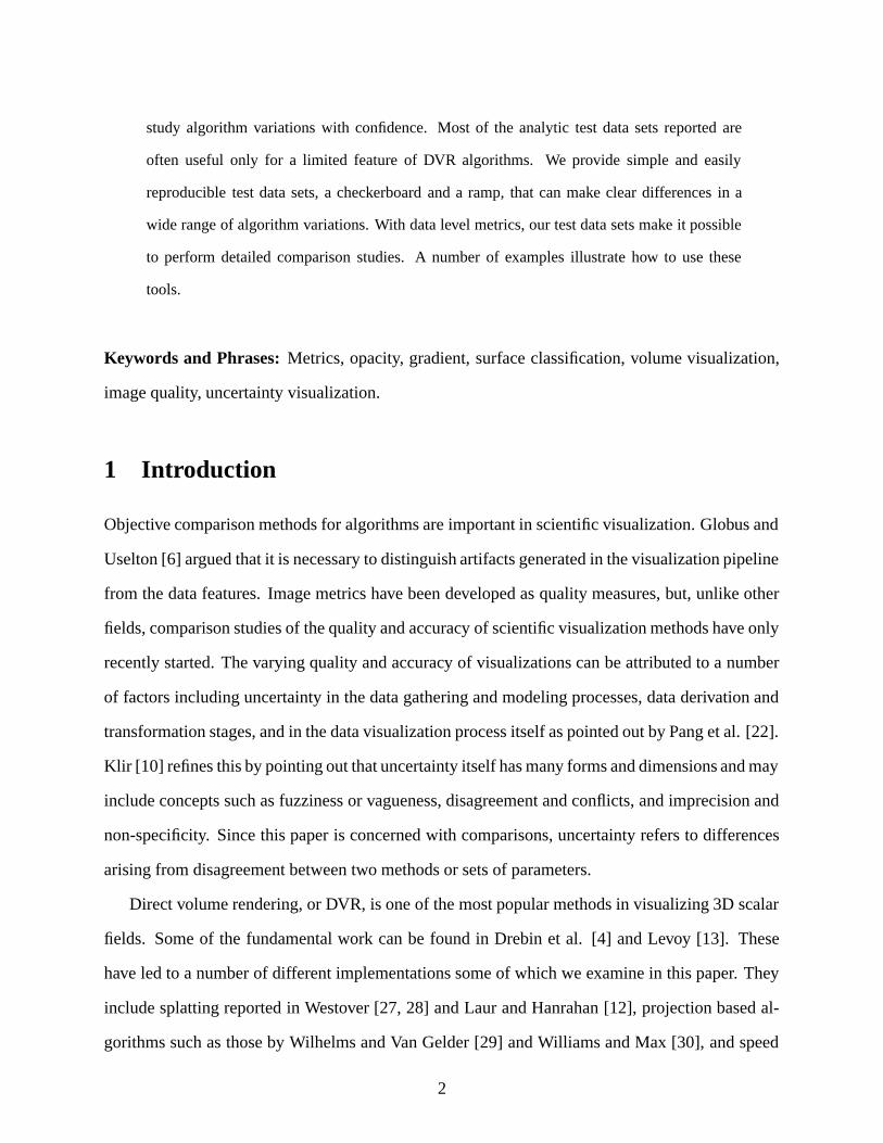
A B C D E

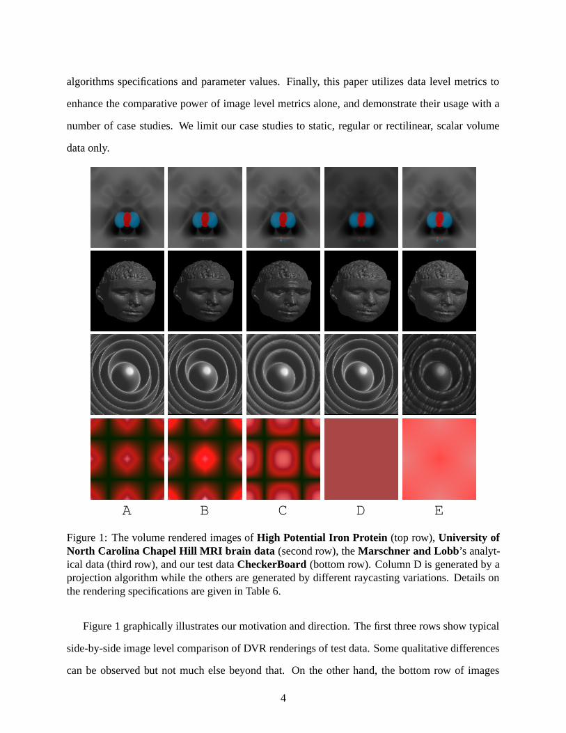
Figure 1: The volume rendered images of High Potential Iron Protein (top row), University ofNorth Carolina Chapel Hill MRI brain data (second row), the Marschner and Lobb’s analyt-ical data (third row), and our test data CheckerBoard (bottom row). Column D is generated by aprojection algorithm while the others are generated by different raycasting variations. Details onthe rendering specifications are given in Table 6.

Figure 1 graphically illustrates our motivation and direction. The first three rows show typical

side-by-side image level comparison of DVR renderings of test data. Some qualitative differences

can be observed but not much else beyond that. On the other hand, the bottom row of images

4

show DVR renderings using one of our test data sets. The qualitative differences are much more

obvious. And because the structure of the data is understood, one can get a better idea of what

the algorithm is doing. Later in the paper, we illustrate how quantitative measures can be obtained

using data level metrics that allow one to get a deeper understanding of the effects of different

algorithm specifications and rendering parameters. The new datasets and metrics highlight differ-

ences between algorithms. In real datasets there will be subtle differences, but it will be hard to

say what is superior. These tools make it clear why the differences exist. It is up to the developer

to determine the appropriate trade-offs for their applications and datasets.

For the rest of this paper, we discuss: relevant previous work and an overview of the com-

parison process; a list of rendering parameters and specifications with an example taxonomy of

DVR algorithms; test data sets; comparison metrics; results on three different comparisons; and

conclusions.

2 Previous Work

The importance of comparing DVR algorithms has long been recognized, but efforts are few and

far in between. Previous work in comparing the quality of DVR algorithms can be grouped into

four general approaches. The first approach compares two or more DVR images using a barrage of

image based metrics such as those used by Neumann [20] and Wittenbrink and Somani [33]. How-

ever, one must be aware of the limitations in popular summary image statistics such as mean square

errors (MSE) and root mean square error (RMSE) as pointed out by Williams and Uselton [31]. For

example, these measures cannot distinguish between noise in image versus structural differences in

image. On the other hand, spatial structure based metrics such as those proposed by Sahasrabudhe

et al. [23], measure and highlight the extent of the inherent structures in the difference between

images. Similarly, the wavelet based perceptual metrics proposed earlier by Gaddipatti et al. [5]

take into account the frequency response of the human visual system on saliency measurements

between two images to help steer further image generation. While these metrics may aid in the

5

analyses of data sets using a particular volume renderer, they are not designed to bring out the

differences caused by variations in different volume renderers or different algorithm settings.

The second approach compares raw data and intermediate information gathered during the ren-

dering process. Since this approach uses more information than the image level approach, it can

provide additional comparative information, and can potentially identify reasons behind differ-

ences in DVR images. Aside from comparing DVR algorithms [8, 9], data level comparison has

also been used for scalar data sets by Sahasrabudhe et al. [23] and vector data sets by Pagendarm

and Post [21]. While this approach is promising, it also has a limitation. It may not be possible to

use such an approach directly for some problems. For example, with DVR comparisons, a common

base algorithm is necessary for collecting common comparison metrics [8, 9].

The third approach uses analytical methods to calculate the error bounds of an algorithm. Rep-

resentative work in this area includes analysis of errors in gradient calculations by Bentum et al.

[2], analysis of normal estimation schemes by Moller et al. [18], and errors in filtering and recon-

struction operations [1, 14, 16, 19, 20, 28, 33]. The limitation of an error bound is the difficulty of

gauging the actual effects directly on a visualization.

The fourth approach compares renderers by using test data to highlight differences. For exam-

ple, researchers have used points and lines [20], cones and pyramids with slots [24, 26], spheres

and cubes [32, 33], analytical functions [16, 19], and tori [7]. The analytical data set introduced

by Marschner and Lobb [16] has also been used in comparisons of gradient filters by Moller et al.

[19]. Other examples include the CT scanned Head (University of North Carolina Chapel Hill), the

Visible Human Project’s data and molecular simulations data such as Hipip (High Potential Iron

Protein) [11, 13, 29]. While using real world data tests nuances in the interaction of an algorithm

with complex data, it makes the comparison of algorithm and parameter effects more difficult. On

the other hand, having simple or analytically defined test data provides a straight forward means

for computing reference solutions, and can facilitate comparisons.

6

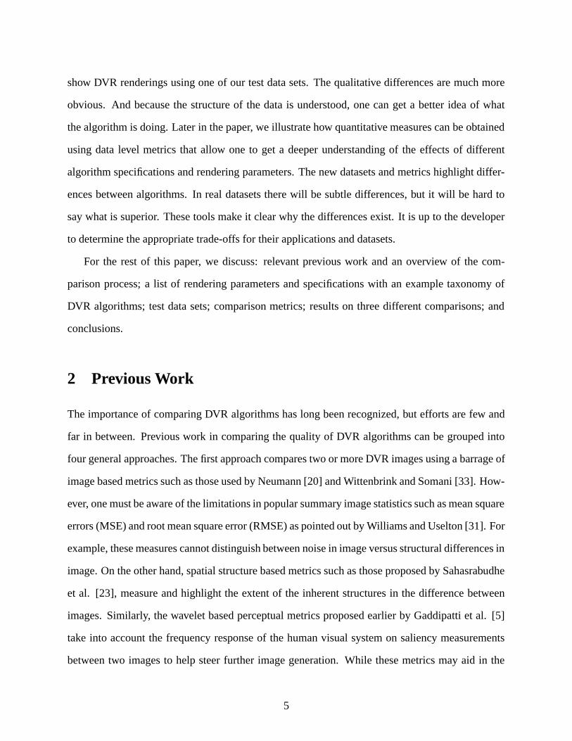
3 Comparison Study Overview

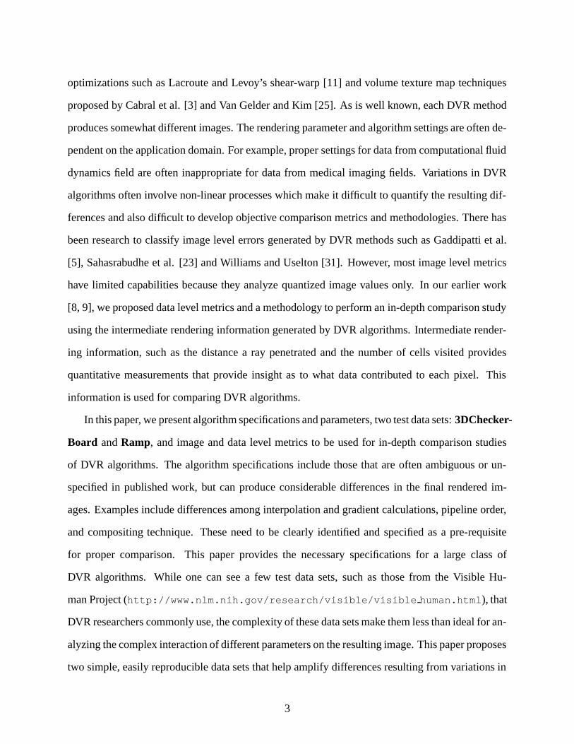
The comparison architecture in Figure 2 allows us to compare DVR algorithms in two different

ways. In Figure 2a, either the algorithm or relevant parts of the rendering parameters (described in

Section 4) are held constant to study the effects of the free variable. For example, effects of differ-

ent DVR implementations can be compared by running them on the same input data and the same

set of rendering parameters. The resulting images are then compared using image level compari-

son techniques. This is the more traditional approach for comparing DVR images and algorithms.

Some obvious limitations of this approach are that comparisons are performed on quantized image

values rather than higher precision intermediate data values. Furthermore, the process by which

those image values are arrived at are totally ignored in image based comparison. Hence, we com-

plement image based comparisons with data level comparisons by comparing intermediate data.

Parameters Data

Algorithm

part 1

Algorithm

part N

Specification

part 1

Specification

part N

IntermediateData

Visual

ComparisonImage Rendered

Image

Mappings

Algorithms

RenderedImage

Parameters Data

(a) (b)

Figure 2: Overview of comparison strategies for DVR images and algorithms.

Figure 2b shows our proposed approach for comparing DVR images and algorithms. The hard-

coded DVR algorithm implementation in Figure 2a is replaced with a generalized DVR algorithm

implementation, described in [8, 9]. Different DVR algorithms are simulated by selection of dif-

ferent algorithm specifications (described in Section 4). The main advantage of this approach is

as DVR algorithms are emulated their intermediate data are available. This allows one to quickly

7

explore DVR algorithms variations through data level comparisons.

Details of how the generalized DVR algorithm in Figure 2b is implemented can be found in

[8, 9]. Essentially, because there is a large variation in different DVR implementations, a base

or reference approach is first selected. The base algorithm may either be projection based or ray

based. For example, Van Gelder and Kim’s [25] 3D volume texture algorithm can be simulated

using a raycasting base algorithm. 3D volume texture algorithm takes parallel slices of equal

thickness from the volume and composites them into the final image. This can be simulated with

regularly sampled rays starting with the first slice [9]. Instead of a raycasting base algorithm,

a projection based algorithm can also be used to simulate other DVR algorithms [8]. The key

component is a software volume scan conversion procedure used originally in Wilhelms and Van

Gelder’s [29] coherent projection. It scan converts the depth information behind each projected

polygon. Interpolated data and color samples used in raycasting can be accounted for by integrating

the values at each scan converting step. Once a base algorithm is selected, the algorithms to be

compared are then faithfully simulated using the base algorithm. Intermediate information such as

number of samples, distance traveled into the volume, accumulated opacities at each point along

the ray are collected and compared. These can also be presented using visual mappings with

standard visualization techniques such as pseudocoloring, iso-surfaces, glyphs, and textures. In

this way, we can evaluate the differences in algorithms systematically and categorically using both

image and data level comparison techniques.

4 Rendering Parameters and DVR Algorithm Specifications

Rigorous parameter and algorithm specifications are pre-requisites for comparison studies of vol-

ume rendered images. In Williams and Uselton’s work [31], they recognized the importance of

this issue and gave a listing of rendering parameters that need to be specified in order to generate

volume rendered images amenable for comparison. However, they did not include the algorithm

specifications which they referred to as implementation details of a volume rendering system. In

8

this paper, we make explicit distinctions between these two groups and refer to them as rendering

parameters and algorithm specifications.

4.1 Rendering Parameters

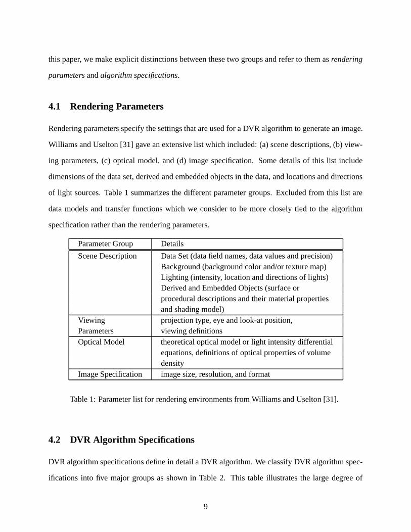
Rendering parameters specify the settings that are used for a DVR algorithm to generate an image.

Williams and Uselton [31] gave an extensive list which included: (a) scene descriptions, (b) view-

ing parameters, (c) optical model, and (d) image specification. Some details of this list include

dimensions of the data set, derived and embedded objects in the data, and locations and directions

of light sources. Table 1 summarizes the different parameter groups. Excluded from this list are

data models and transfer functions which we consider to be more closely tied to the algorithm

specification rather than the rendering parameters.

Parameter Group Details

Scene Description Data Set (data field names, data values and precision)Background (background color and/or texture map)Lighting (intensity, location and directions of lights)Derived and Embedded Objects (surface orprocedural descriptions and their material propertiesand shading model)

Viewing projection type, eye and look-at position,Parameters viewing definitionsOptical Model theoretical optical model or light intensity differential

equations, definitions of optical properties of volumedensity

Image Specification image size, resolution, and format

Table 1: Parameter list for rendering environments from Williams and Uselton [31].

4.2 DVR Algorithm Specifications

DVR algorithm specifications define in detail a DVR algorithm. We classify DVR algorithm spec-

ifications into five major groups as shown in Table 2. This table illustrates the large degree of

9

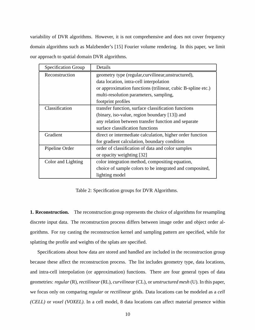
variability of DVR algorithms. However, it is not comprehensive and does not cover frequency

domain algorithms such as Malzbender’s [15] Fourier volume rendering. In this paper, we limit

our approach to spatial domain DVR algorithms.

Specification Group Details

Reconstruction geometry type (regular,curvilinear,unstructured),data location, intra-cell interpolationor approximation functions (trilinear, cubic B-spline etc.)multi-resolution parameters, sampling,footprint profiles

Classification transfer function, surface classification functions(binary, iso-value, region boundary [13]) andany relation between transfer function and separatesurface classification functions

Gradient direct or intermediate calculation, higher order functionfor gradient calculation, boundary condition

Pipeline Order order of classification of data and color samplesor opacity weighting [32]

Color and Lighting color integration method, compositing equation,choice of sample colors to be integrated and composited,lighting model

Table 2: Specification groups for DVR Algorithms.

1. Reconstruction. The reconstruction group represents the choice of algorithms for resampling

discrete input data. The reconstruction process differs between image order and object order al-

gorithms. For ray casting the reconstruction kernel and sampling pattern are specified, while for

splatting the profile and weights of the splats are specified.

Specifications about how data are stored and handled are included in the reconstruction group

because these affect the reconstruction process. The list includes geometry type, data locations,

and intra-cell interpolation (or approximation) functions. There are four general types of data

geometries: regular (R), rectilinear (RL), curvilinear (CL), or unstructured mesh (U). In this paper,

we focus only on comparing regular or rectilinear grids. Data locations can be modeled as a cell

(CELL) or voxel (VOXEL). In a cell model, 8 data locations can affect material presence within

10

a cell and the data values are interpolated at intra-cell locations. Trilinear (TL) interpolation is

typically used for intra-cell interpolation but some higher order functions are also used. In a voxel

model, materials are centered around data locations. Various types of distance functions are used

to calculate the influence (or footprints for object order algorithms) of a voxel. In this paper, we

use the smoothness (or continuity) and the order of the error function (EF) to specify the higher

order reconstruction functions as in Moller et al. [19]. For example, we can use a cubic function

that is C2 continuous and has an EF order of 2 for intra-cell interpolations.

Sampling pattern refers to any description regarding the distributions of sampled points in the z

direction of the viewing coordinate system. There are three basic types: regular sampling (REG),

cell face sampling (CF), and volume slicing (VS). Together with the sampling pattern, the threshold

condition for terminating the rays should also be specified.

Projection based algorithms such as coherent projection and splatting use either cell projections

(CELL PROJECTION) or Gaussian (GAUSSIAN) footprints to composite material contributions

from a cell (or voxel) to the screen. A set of polygons are often used to approximate the influence

from a voxel (or cell). The profiles of the set of polygons should be specified along with any

approximation functions used for the material accumulations.

2. Classification. The classification group refers to mapping methods that map data values to

different materials or surfaces. It includes transfer functions, and surface classification functions.

The data values are typically mapped to color (red, green, blue) and opacity values. A subtle dis-

tinction should be made in how the colors in the classification functions are defined. In associative

(AS) classification (or transfer) functions, a user defines RGB values to be influenced by opacity

values. The intensities of RGB components are dependent on the opacity function defined, which

seems to be the majority of the cases. In non-associative (NAS) functions, intensities of RGB

components are independent of opacity values. In other words, NAS or AS specifies whether the

transfer function for color and opacity channel have the same scalar domain or not. Users should

define RGB intensities as material properties and opacity acts only as an occlusion factor at the

11

sample points. However, the opacity components affect the RGB intensities of samples when the

color is integrated over a distance. This is also related to color integration and compositing equa-

tion specifications. Some published work does not make a clear distinction in this category. We

will clear some of these up using a taxonomy of algorithms later in this section. Most algorithms

use one of three volume surface classifications: Binary, Iso-value Contour Surface or Levoy’s [13]

Region Boundary Surface classifications. In Binary classification, a surface is defined if the data

value falls within a specified range. For Iso-value Contour and Region Boundary surfaces, a sur-

face is defined as a function of data value and its gradient. In Iso-value Contour, a fuzzy surface

is created around a single iso-value. On the other hand, in Region Boundary, transitions among

multiple surfaces can be defined.

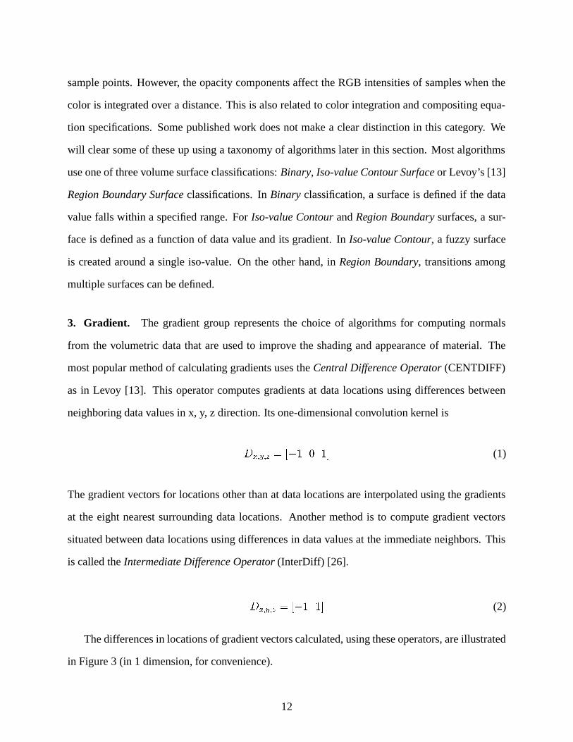
3. Gradient. The gradient group represents the choice of algorithms for computing normals

from the volumetric data that are used to improve the shading and appearance of material. The

most popular method of calculating gradients uses the Central Difference Operator (CENTDIFF)

as in Levoy [13]. This operator computes gradients at data locations using differences between

neighboring data values in x, y, z direction. Its one-dimensional convolution kernel is

Dx;y;z = [�1 0 1] (1)

The gradient vectors for locations other than at data locations are interpolated using the gradients

at the eight nearest surrounding data locations. Another method is to compute gradient vectors

situated between data locations using differences in data values at the immediate neighbors. This

is called the Intermediate Difference Operator (InterDiff) [26].

Dx;y;z = [�1 1] (2)

The differences in locations of gradient vectors calculated, using these operators, are illustrated

in Figure 3 (in 1 dimension, for convenience).

12

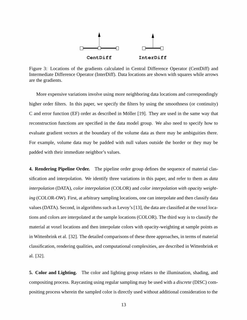
CentDiff InterDiff

Figure 3: Locations of the gradients calculated in Central Difference Operator (CentDiff) andIntermediate Difference Operator (InterDiff). Data locations are shown with squares while arrowsare the gradients.

More expensive variations involve using more neighboring data locations and correspondingly

higher order filters. In this paper, we specify the filters by using the smoothness (or continuity)

C and error function (EF) order as described in Moller [19]. They are used in the same way that

reconstruction functions are specified in the data model group. We also need to specify how to

evaluate gradient vectors at the boundary of the volume data as there may be ambiguities there.

For example, volume data may be padded with null values outside the border or they may be

padded with their immediate neighbor’s values.

4. Rendering Pipeline Order. The pipeline order group defines the sequence of material clas-

sification and interpolation. We identify three variations in this paper, and refer to them as data

interpolation (DATA), color interpolation (COLOR) and color interpolation with opacity weight-

ing (COLOR-OW). First, at arbitrary sampling locations, one can interpolate and then classify data

values (DATA). Second, in algorithms such as Levoy’s [13], the data are classified at the voxel loca-

tions and colors are interpolated at the sample locations (COLOR). The third way is to classify the

material at voxel locations and then interpolate colors with opacity-weighting at sample points as

in Wittenbrink et al. [32]. The detailed comparisons of these three approaches, in terms of material

classification, rendering qualities, and computational complexities, are described in Wittenbrink et

al. [32].

5. Color and Lighting. The color and lighting group relates to the illumination, shading, and

compositing process. Raycasting using regular sampling may be used with a discrete (DISC) com-

positing process wherein the sampled color is directly used without additional consideration to the

13

sampling distances. However, when samples are taken at non-regular distances (such as CF sam-

pling), the inter-sample distances are considered and integrated (INTEG) along the path between

sample colors. In some algorithms, a constant (CONST) is multiplied to adjust the color intensi-

ties. One way to visualize sampled volume data is to use a simple method such as the maximum

intensity projection (MIP). However, in most of DVR algorithms, sample colors are composited.

When the color is composited in back-to-front (BF) or front-to-back (FB) order, different DVR

algorithms choose either a single color (SINGLE) of the current sample point or an average of

two colors (AVERAGING) to represent the sampling interval. The latter choice tends to result in

smoother images. Sampled colors can be composited using associated (AS) (Equation 3) or non-

associated (NAS) (Equation 4) color compositing equations (comp eq). Different compositing

approaches can be shown to be the result of different particle models such as Max’s [17] absorp-

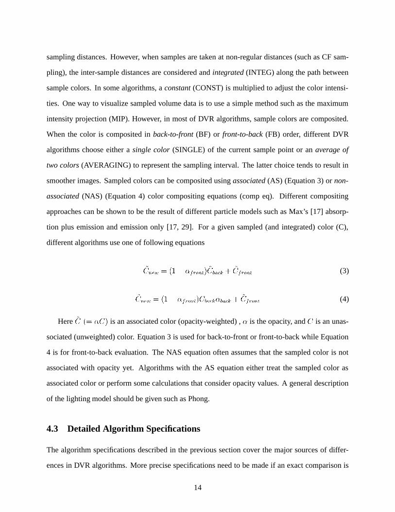
tion plus emission and emission only [17, 29]. For a given sampled (and integrated) color (C),

different algorithms use one of following equations

~Cnew = (1� �front) ~Cback + ~Cfront (3)

~Cnew = (1� �front)Cback�back + ~Cfront (4)

Here ~C (= �C) is an associated color (opacity-weighted) , � is the opacity, and C is an unas-

sociated (unweighted) color. Equation 3 is used for back-to-front or front-to-back while Equation

4 is for front-to-back evaluation. The NAS equation often assumes that the sampled color is not

associated with opacity yet. Algorithms with the AS equation either treat the sampled color as

associated color or perform some calculations that consider opacity values. A general description

of the lighting model should be given such as Phong.

4.3 Detailed Algorithm Specifications

The algorithm specifications described in the previous section cover the major sources of differ-

ences in DVR algorithms. More precise specifications need to be made if an exact comparison is

14

desired. However, it may not be always possible to achieve this. For example, when volume cells

are projected, the projected polygons are likely to be rendered in hardware. Rendering results vary

depending on the hardware scan conversions where detailed specifications are often hard to obtain.

Fortunately, software simulations of the scan conversion process can standardize such hardware

dependencies and bound the discrepancies to within a certain range. For example, we simulated

the coherent projection algorithm and measured the differences between color values in all the ver-

tices of all the projected polygons with the original algorithm [8]. The differences were less than

10�7 in the scale of 0.0 to 1.0 for each color channel (in multiple viewing directions) effectively

machine epsilon for a single precision floating point value. Another example of detailed algorithm

specification would be the precision of color compositing. A lower precision of the opacity chan-

nel can produce dramatically different rendering results. It is important to make efforts to have a

complete specification of all the rendering parameters and algorithm specifications.

4.4 Taxonomy

algorithm data location pipeline order sampling tr fn footprint

Levoy [13] CELL COLOR REG NASCoherent Proj. [29] CELL, VOXEL DATA CF NAS CELLSplatting [12, 27] VOXEL DATA AS GAUSSIANShear-warp [11] CELL COLOR CF NASVoltx [25] CELL, VOXEL COLOR VS NASOpacity-Weighting [32] CELL, VOXEL COLOR-OW R AS

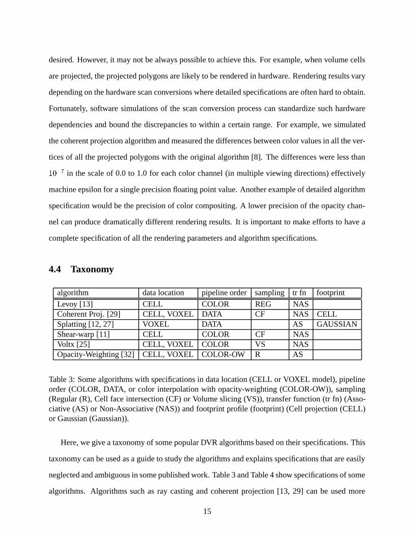
Table 3: Some algorithms with specifications in data location (CELL or VOXEL model), pipelineorder (COLOR, DATA, or color interpolation with opacity-weighting (COLOR-OW)), sampling(Regular (R), Cell face intersection (CF) or Volume slicing (VS)), transfer function (tr fn) (Asso-ciative (AS) or Non-Associative (NAS)) and footprint profile (footprint) (Cell projection (CELL)or Gaussian (Gaussian)).

Here, we give a taxonomy of some popular DVR algorithms based on their specifications. This

taxonomy can be used as a guide to study the algorithms and explains specifications that are easily

neglected and ambiguous in some published work. Table 3 and Table 4 show specifications of some

algorithms. Algorithms such as ray casting and coherent projection [13, 29] can be used more

15

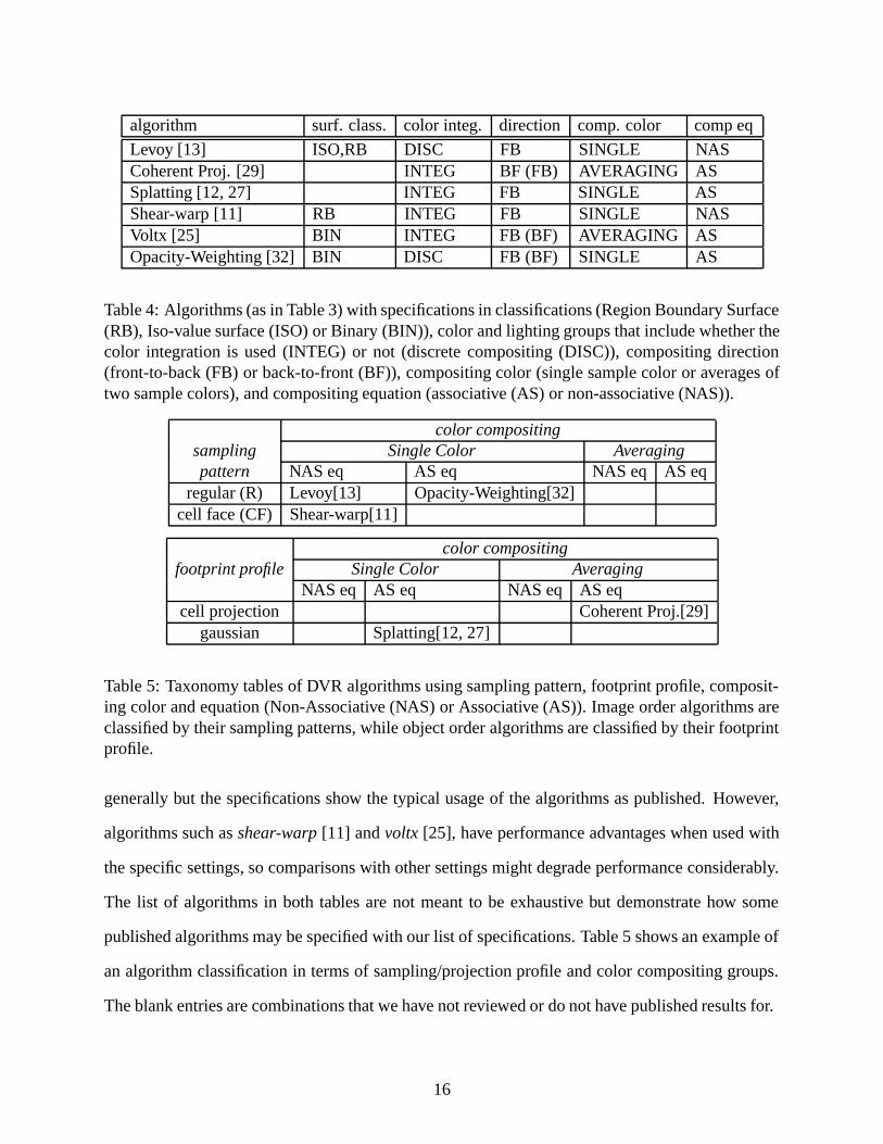
algorithm surf. class. color integ. direction comp. color comp eq

Levoy [13] ISO,RB DISC FB SINGLE NASCoherent Proj. [29] INTEG BF (FB) AVERAGING ASSplatting [12, 27] INTEG FB SINGLE ASShear-warp [11] RB INTEG FB SINGLE NASVoltx [25] BIN INTEG FB (BF) AVERAGING ASOpacity-Weighting [32] BIN DISC FB (BF) SINGLE AS

Table 4: Algorithms (as in Table 3) with specifications in classifications (Region Boundary Surface(RB), Iso-value surface (ISO) or Binary (BIN)), color and lighting groups that include whether thecolor integration is used (INTEG) or not (discrete compositing (DISC)), compositing direction(front-to-back (FB) or back-to-front (BF)), compositing color (single sample color or averages oftwo sample colors), and compositing equation (associative (AS) or non-associative (NAS)).

color compositingsampling Single Color Averagingpattern NAS eq AS eq NAS eq AS eq

regular (R) Levoy[13] Opacity-Weighting[32]cell face (CF) Shear-warp[11]

color compositingfootprint profile Single Color Averaging

NAS eq AS eq NAS eq AS eqcell projection Coherent Proj.[29]

gaussian Splatting[12, 27]

Table 5: Taxonomy tables of DVR algorithms using sampling pattern, footprint profile, composit-ing color and equation (Non-Associative (NAS) or Associative (AS)). Image order algorithms areclassified by their sampling patterns, while object order algorithms are classified by their footprintprofile.

generally but the specifications show the typical usage of the algorithms as published. However,

algorithms such as shear-warp [11] and voltx [25], have performance advantages when used with

the specific settings, so comparisons with other settings might degrade performance considerably.

The list of algorithms in both tables are not meant to be exhaustive but demonstrate how some

published algorithms may be specified with our list of specifications. Table 5 shows an example of

an algorithm classification in terms of sampling/projection profile and color compositing groups.

The blank entries are combinations that we have not reviewed or do not have published results for.

16

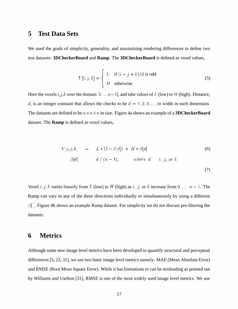
5 Test Data Sets

We used the goals of simplicity, generality, and maximizing rendering differences to define two

test datasets: 3DCheckerBoard and Ramp. The 3DCheckerBoard is defined as voxel values,

V [i; j; k] =

8>><>>:L if (i + j + k)=d is odd

H otherwise(5)

Here the voxels i,j,k over the domain [0 : : : n�1], and take values of L (low) orH (high). Distance,

d, is an integer constant that allows the checks to be d = 1; 2; 3; : : : in width in each dimension.

The datasets are defined to be n�n�n in size. Figure 4a shows an example of a 3DCheckerBoard

dataset. The Ramp is defined as voxel values,

V [i; j; k] = L � (1� �[d]) + H � �[d] (6)

�[d] = d = (n� 1); where d = i; j; or k

(7)

Voxel i; j; k varies linearly from L (low) to H (high) as i; j; or k increase from 0 : : : n � 1. The

Ramp can vary in any of the three directions individually or simultaneously by using a different

�[ ]. Figure 4b shows an example Ramp dataset. For simplicity we do not discuss pre-filtering the

datasets.

6 Metrics

Although some new image level metrics have been developed to quantify structural and perceptual

differences [5, 23, 31], we use two basic image level metrics namely: MAE (Mean Absolute Error)

and RMSE (Root Mean Square Error). While it has limitations or can be misleading as pointed out

by Williams and Uselton [31], RMSE is one of the most widely used image level metrics. We use

17

(a) 3DCheckerBoard (b) Ramp

Figure 4: Test data example shown in cell model; (a) 3DCheckerBoard (n = 4; d = 1). Theblack and white sphere show the high (H) and low (L) value. (b) Ramp (n = 4). The data valueschanges from the maximum (black) to the minimum (white). The interior data points are omittedto reduce clutter in these illustrations.

MAE as an additional image metric. These are defined below:

RMSE =sX

i;j

[A(i; j)�B(i; j)]2=N2

MAE =Xi;j

jA(i; j)�B(i; j)j=N2

where A and B are images (of size N �N ) to be compared.

We include these image level summary statistics for measuring general differences as a point

of reference and because they are well known. Perceptual image metrics are not included because

the test data sets are already supposed to highlight differences in the algorithms. In fact, one

can easily observe structural patterns in the images in the next section. Perceptual metrics would

simply produce high values for such images with obvious spatial structures. Hence, the primary

metrics that we use in Section 7 are data level metrics. Several types of data level metrics that

utilize intermediate data were introduced in [8, 9]. Recall that in order to collect data level metrics

that can be compared across different classes of DVR algorithms, the algorithms to be compared

must first be simulated by a common base algorithm. This step also ensures that the intermediate

rendering data are registered and ready for comparison.

In this paper, we use several threshold based metrics such as NS (Number of Samples), NSD

18

(a) (b) (c) (d)

Figure 5: DVR images (top row) with corresponding visualizations for the number of samples (NS)metric (bottom row). NS is accumulated until the given opacity threshold is reached for each pixelat (a) 0.10, (b) 0.15, (c) 0.20, and (d) 0.30. Regular ray sampling is used to render this Hipip dataset. Black regions indicate that rays entered and exited the volume without reaching the opacitythreshold.

(Number of Samples Differences) which measure the difference in the number of samples, and

Corr (Correlation of sampled colors) which measures how well correlated are the values used in

arriving at a pixel color. These metrics are called threshold based because they are collected as

long as a specified threshold has not been reached. For example, NS counts the number of values

contributing to a pixel color while the ray has not reached an opacity threshold.

Figure 5 compares the number of sample metric on the Hipip data set with four different opacity

thresholds. A rainbow color map is used for each threshold to show fewer samples (blue) to many

samples (red).

To calculate the correlation between two vectors of sample colors collected by two different

algorithms, we let V and W be two random variables representing the two normalized sample

color vectors along the viewing direction. The statistical correlation � between these two random

variables is defined by

�(~V ; ~W ) =cov(~V ; ~W )

�V �W=E[(~V � �V )( ~W � �W )]

�V �W(8)

19

where cov(V;W ) is the covariance of the two random variables, �V and �W are the means of of ~V

and ~W , E is the expectation, and � denotes standard deviation of the random variable. The closer

� is to 1, the more correlated the two sample color vectors are. The correlation metric (Corr) at

each pixel location may be color mapped (as in Figure 14) or averaged to obtain a mean correlation

value for the entire image (as in Table 9).

Sample colors are usually represented by separate red, green, and blue color and opacity chan-

nels which may or may not be correlated to each other. Hence, the correlation metric is calculated

for three color channels to provide additional information when comparing two different render-

ings.

7 Results

In this section, we present three examples to show how our test data are used in comparison studies

of DVR algorithms using both image and data level metrics. In most of the examples, parallel

projections with simple orthographic views are used. The simple viewing setup coupled with data

sets that are easy to understand helps us in understanding and pinpointing the effects of different

algorithm specifications as discussed in the examples below. That is, the simple viewing setup

produces patterns in the resulting image that can be readily explained given the algorithm speci-

fications. On the other hand, changing the projection from parallel to perspective (see Figure 9)

or changing to a non-orthogonal view (see Figure 10) may be less effective for this task. Another

reason why we do not recommend using perspective projection is because some algorithms, such

as coherent projection, are limited to parallel projections.

When looking at the images in the three examples to follow, the rendered images may appear

to be abstract and not what one might think the data ought to look like. It is because rendering

results of our test data sets can vary widely depending on algorithms and their settings. This is in

fact one of the main reasons for designing test data that are very simple. They immediately bring

these differences to the forefront and raise our attention, whereas more complex data set renderings

20

would not be easy to interpret. Furthermore, because we know the simple structure of the data sets,

the appearance of the renderings directly helps us explain the effects of the different algorithm

specifications. This is achieved with the aid of data level metrics as described in the examples

below. Of course, as can be seen in the images in this section, some of the differences are more

significant than others. The ability to alter one or more algorithm specification at a time, allows us

to determine which combinations have more impact on the resulting images.

7.1 Pipeline Order, Compositing, Data Model

In this example, we experimented with variations in specification groups such as data model, ren-

dering pipeline order, and color integration. Variations in algorithm specifications are given in

Table 6. Other specifications such as sampling patterns are held constant and their details are de-

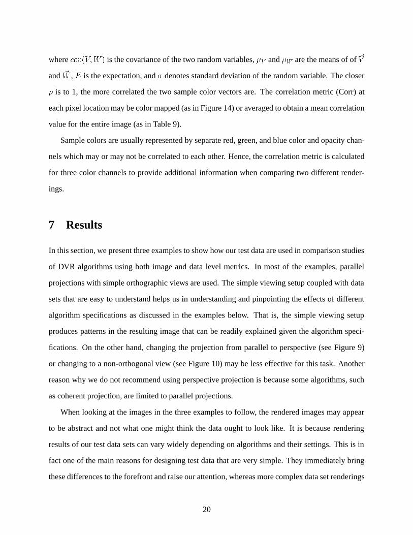
scribed in the Appendix (Figure 17). Figure 6 shows the rendered images of 3DCheckerBoard

with different algorithm variations (A to E) and their corresponding difference images (F to I). The

difference images use image A as the reference image to be compared. The data set used is a 33

3DCheckerBoard. The transfer function and the actual data are described in the Appendix. The

volume data is rendered with a cell model.

image algorithm data model pipeline order color integ comp color

A raycasting tri-linear DATA INTEG AVERAGINGB raycasting tri-linear DATA INTEG SINGLEC raycasting cubic filter DATA INTEG AVERAGINGD Coherent Proj. [29] tri-linear DATA INTEG AVERAGINGE Levoy [13] tri-linear COLOR DISCRETE SINGLE

Table 6: Specifications for the algorithms that generated images A to E in Figure 6.

An obvious difference can be noticed by simply changing the order of operations in the pipeline.

For example, interpolated data values are used to index into a transfer function in images A, B, C

while data values are converted to color values and then interpolated in image E. By interpolating

data values first, and in combination with a transfer function, a full range of material can be ex-

tracted from this simple data set. On the other hand, by converting data to color values first, we

21

A B E

F: |B − A|

C D

G: |C − A| H: |D − A| I: |E − A|

colormap

Figure 6: The volume rendered images of the 3DCheckerBoard data with different specificationsettings. Images A to E (Same as the bottom row of Figure 1) are generated by DVR algorithmswith specifications given in Table 6. Image F to I are differences of B to E with the reference imageA respectively. All images are 256� 256. The color map for the transfer function is also displayedabove images and its details are provided in the Appendix.

are essentially seeing the blending of only two materials – either red or white in image E. Image

D, produced by Coherent Projection, appears as a homogeneous block because in this view, the

volume cells are projected into four abutting square polygons where the colors at the vertices of

each projected polygon are averaged between the front and back colors (materials). These colors

are either red or white. Hence, the interpolated colors for each polygon are homogeneous. In ad-

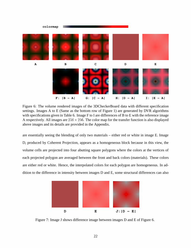
dition to the difference in intensity between images D and E, some structural differences can also

D E J:|D − E|

Figure 7: Image J shows difference image between images D and E of Figure 6.

22

be seen in their difference image as illustrated in Figure 7. This can be attributed to the fact that

the algorithm for image E uses a discrete color integration and compositing with a single sampled

color, while the algorithm for image D uses the averaged color of the front and back samples along

the ray.

Both algorithms for images A and B use data interpolation (tri-linear) at the sample points.

The difference stems from the choice of color to be composited (comp color). Algorithm A uses

averaged values between two samples (such as front and back values) while the one for B uses a

single sample value. The differences are more subtle and the resulting difference image (see image

F) as well as summary statistics on the comparison also yield the least difference (see Figure 8).

One can see a more noticeable difference between images A and C, where the type of interpolation

function is different while the other algorithms specifications are held constant. Image C is gener-

ated with a cubic filter function while image A is generated with a tri-linear interpolation function.

This results in a smoother transition of intensity from the data value to the cell boundary.

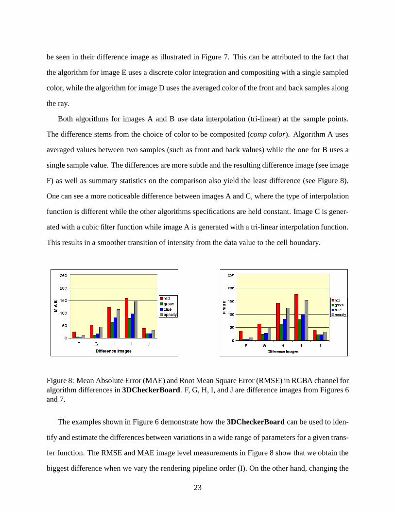
Figure 8: Mean Absolute Error (MAE) and Root Mean Square Error (RMSE) in RGBA channel foralgorithm differences in 3DCheckerBoard. F, G, H, I, and J are difference images from Figures 6and 7.

The examples shown in Figure 6 demonstrate how the 3DCheckerBoard can be used to iden-

tify and estimate the differences between variations in a wide range of parameters for a given trans-

fer function. The RMSE and MAE image level measurements in Figure 8 show that we obtain the

biggest difference when we vary the rendering pipeline order (I). On the other hand, changing the

23

choice of color compositing (F) produced the least difference.

We reiterate why it is important to use simple data sets in analyzing different algorithm vari-

ations. Figure 1 shows how our test data set compares to Marschner and Lobb’s test data for the

same example as Figure 6. Our test data more clearly indicates differences amongst the varia-

tions. Furthermore, it is also important to use viewing parameters that do not unduly complicate

the analysis.

So far we have used a simple orthogonal view using parallel projection to clearly demonstrate

the effectiveness of our test data. However, one can do a similar analysis using different settings for

a more complete comparison study of algorithms. Figure 9 illustrates what happens with perspec-

tive projection, and Figure 10 compares non-orthogonal views. The differences among algorithms

in Figure 9 are not as dramatic. Minimal additional information about the algorithm is gained by

the perspective views, and they complicate the analysis task. In image D of Figure 10, Coherent

Projection shows more material content because each volume cell is projected into more than one

polygon. While additional information is made available in the images, the patterns in the resulting

images are highly dependent on the viewing angle, and also complicates the analysis task.

A B C Eview

Figure 9: Renderings of algorithm A, B, C, and E using a perspective view.

7.2 Surface Classifications

In this example, we demonstrate how the Ramp data with n = 4 can be used to study variations

in surface classification functions. The data has a minimum of zero and maximum of 255 and

changes linearly along the x-direction (from the left to the right in the images). The detailed

specifications of the surface classifications are described by Table 10 to 13 in the Appendix. We

24

A D |D − A|

Figure 10: Renderings of algorithm A and D using a non-orthogonal viewing angle.

used a raycasting algorithm for this example. All images (256� 256) are generated with identical

algorithm specifications except for those specified in Table 7. Binary Surface classifications are

compared with other similarly defined surface classifications. We highlight some areas of interest

with rectangular boxes.

Image Index pipe order surf. classification

A DATA BinaryB COLOR Region Boundary

C DATA BinaryD DATA Iso-value Contour

Table 7: DVR pipeline order and surface classification methods for the images in Figure 11.

Binary classification is used in Figure 11 A. That is, any data between 127 to 255 are classified

as a certain material, while data values between 0 and 126 are treated as empty space. It shows

the location of the volume surface where data values are equal to or higher than 127. Figure 11

B shows the corresponding rendering using Levoy’s [13] Region Boundary Surface classification.

It shows a more gradual transition from the surface material to the empty material boundary. The

light blue lines show the grid lines for i = 1 and i = 2. The last two visualizations on the top

row show data level analyses in the transition region. Figure 11 NSB;�=0:75 shows the number of

samples needed to accumulate up to the opacity of 0.75 at each pixel in Fig. 11 B. The values of

NSB;�=0:75 are mapped to the standard rainbow color map. The black areas indicate the regions

where pixels did not reach the opacity threshold. Closer to the i = 1 grid line, more samples are

25

A B |A − B| NSD α =.95A,BNS Β,α =.75

i=1 i=2

colormapMIN MAX

C D |C − D| NSD α =.75 Corrα =.75C,D C,D

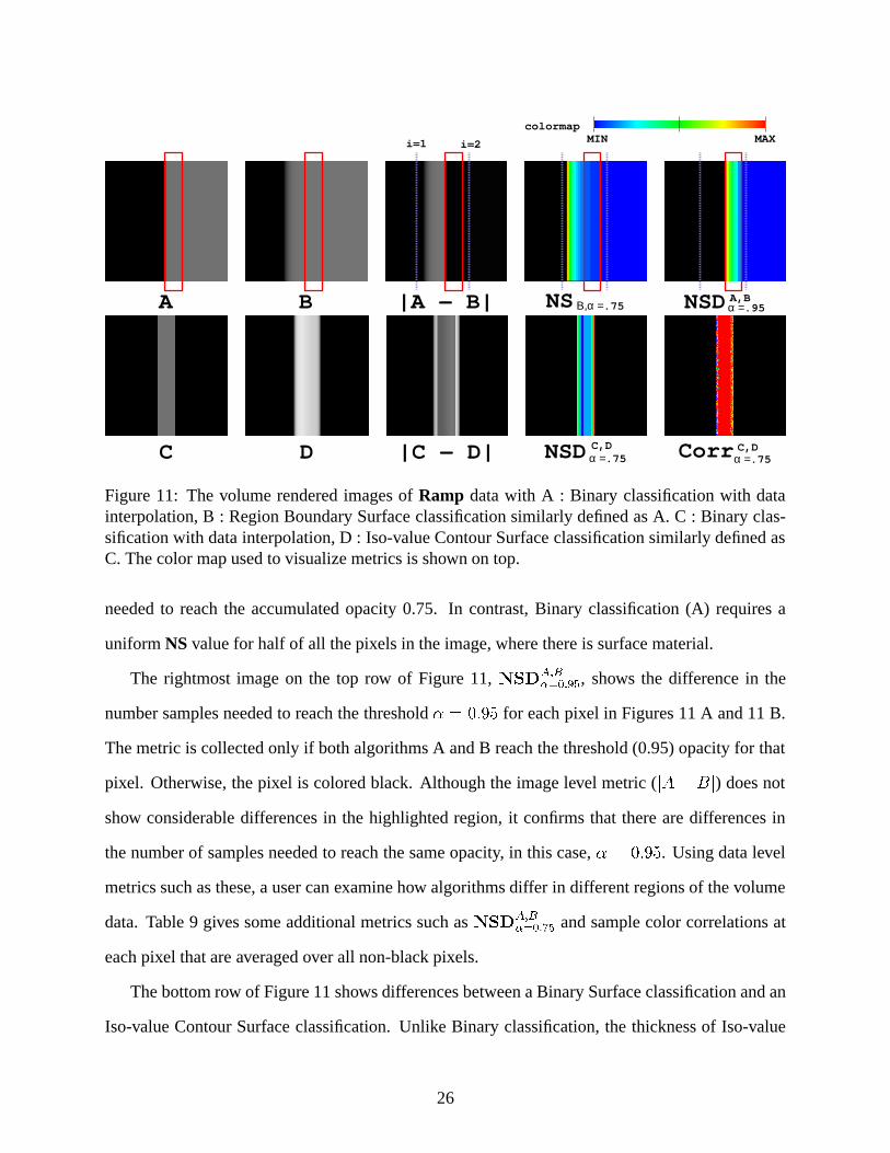
Figure 11: The volume rendered images of Ramp data with A : Binary classification with datainterpolation, B : Region Boundary Surface classification similarly defined as A. C : Binary clas-sification with data interpolation, D : Iso-value Contour Surface classification similarly defined asC. The color map used to visualize metrics is shown on top.

needed to reach the accumulated opacity 0.75. In contrast, Binary classification (A) requires a

uniform NS value for half of all the pixels in the image, where there is surface material.

The rightmost image on the top row of Figure 11, NSDA;B�=0:95, shows the difference in the

number samples needed to reach the threshold � = 0:95 for each pixel in Figures 11 A and 11 B.

The metric is collected only if both algorithms A and B reach the threshold (0.95) opacity for that

pixel. Otherwise, the pixel is colored black. Although the image level metric (jA � Bj) does not

show considerable differences in the highlighted region, it confirms that there are differences in

the number of samples needed to reach the same opacity, in this case, � = 0:95. Using data level

metrics such as these, a user can examine how algorithms differ in different regions of the volume

data. Table 9 gives some additional metrics such as NSDA;B�=0:75 and sample color correlations at

each pixel that are averaged over all non-black pixels.

The bottom row of Figure 11 shows differences between a Binary Surface classification and an

Iso-value Contour Surface classification. Unlike Binary classification, the thickness of Iso-value

26

Contour surface can be controlled by the region transition thickness (r) and gradient magnitude

around surfaces (see Table 13 in the Appendix). The differences can be measured and analyzed

similar to the top row in Figure 11 using both image and data level approaches. Summary statistics

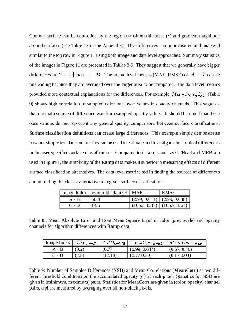
of the images in Figure 11 are presented in Tables 8-9. They suggest that we generally have bigger

differences in jC � Dj than jA � Bj. The image level metrics (MAE, RMSE) of jA � Bj can be

misleading because they are averaged over the larger area to be compared. The data level metrics

provided more contextual explanations for the differences. For example, MeanCorrA;B�=0:75 (Table

9) shows high correlation of sampled color but lower values in opacity channels. This suggests

that the main source of difference was from sampled opacity values. It should be noted that these

observations do not represent any general quality comparisons between surface classifications.

Surface classification definitions can create large differences. This example simply demonstrates

how our simple test data and metrics can be used to estimate and investigate the nominal differences

in the user-specified surface classifications. Compared to data sets such as CTHead and MRBrain

used in Figure 1, the simplicity of the Ramp data makes it superior in measuring effects of different

surface classification alternatives. The data level metrics aid in finding the sources of differences

and in finding the closest alternative to a given surface classification.

Image Index % non-black pixel MAE RMSE

A - B 50.4 (2.99, 0.011) (2.99, 0.036)C - D 14.5 (105.3, 0.87) (105.7, 1.63)

Table 8: Mean Absolute Error and Root Mean Square Error in color (grey scale) and opacitychannels for algorithm differences with Ramp data.

Image Index NSD�=0:75 NSD�=0:95 MeanCorr�=0:75 MeanCorr�=0:95A - B (0,2) (0,7) (0.99, 0.644) (0.67, 0.40)C - D (2,8) (12,18) (0.77,0.30) (0.17,0.03)

Table 9: Number of Samples Differences (NSD) and Mean Correlations (MeanCorr) at two dif-ferent threshold conditions on the accumulated opacity (�) at each pixel. Statistics for NSD aregiven in (minimum, maximum) pairs. Statistics for MeanCorrs are given in (color, opacity) channelpairs, and are measured by averaging over all non-black pixels.

27

7.3 Gradient Calculations

Figure 12 demonstrates a different usage of 3DCheckerBoard for measuring differences between

gradient calculation methods. All images are rendered using the Region Boundary Surface clas-

sification with data interpolation (DATA). This volume surface classification is usually used with

color interpolation as in Lacroute [11] and Levoy [13]. However, we use data interpolation in-

stead to illustrate the differences in the gradient calculation. The viewing direction is orthogonal

to a face of the volume’s bounding box. The data size is 73. The material colors and the surface

classifications are given in Figure 18 of the Appendix.

BA C D

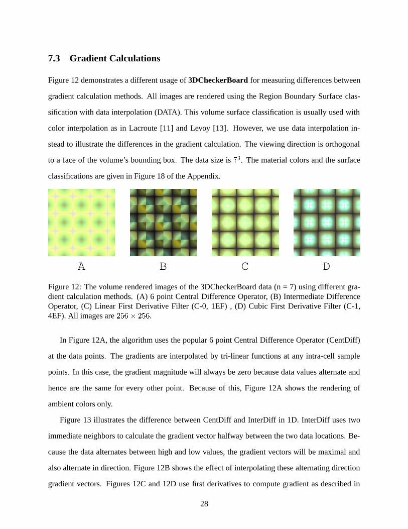
Figure 12: The volume rendered images of the 3DCheckerBoard data (n = 7) using different gra-dient calculation methods. (A) 6 point Central Difference Operator, (B) Intermediate DifferenceOperator, (C) Linear First Derivative Filter (C-0, 1EF) , (D) Cubic First Derivative Filter (C-1,4EF). All images are 256� 256.

In Figure 12A, the algorithm uses the popular 6 point Central Difference Operator (CentDiff)

at the data points. The gradients are interpolated by tri-linear functions at any intra-cell sample

points. In this case, the gradient magnitude will always be zero because data values alternate and

hence are the same for every other point. Because of this, Figure 12A shows the rendering of

ambient colors only.

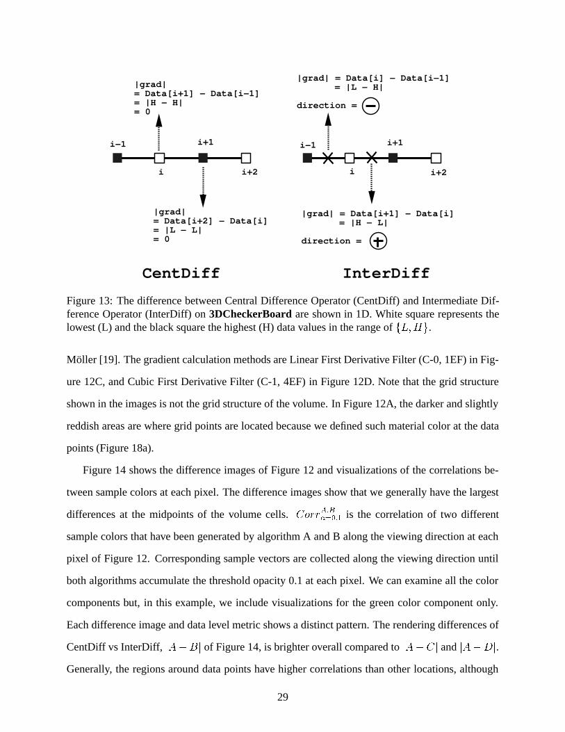
Figure 13 illustrates the difference between CentDiff and InterDiff in 1D. InterDiff uses two

immediate neighbors to calculate the gradient vector halfway between the two data locations. Be-

cause the data alternates between high and low values, the gradient vectors will be maximal and

also alternate in direction. Figure 12B shows the effect of interpolating these alternating direction

gradient vectors. Figures 12C and 12D use first derivatives to compute gradient as described in

28

CentDiff InterDiff

|grad| = Data[i] − Data[i−1] = |L − H|

direction =

|grad| = Data[i+1] − Data[i] = |H − L|

direction =

|grad|= Data[i+1] − Data[i−1]= |H − H|= 0

|grad|= Data[i+2] − Data[i] = |L − L|= 0

i−1

i

i+1

i+2 i

i−1 i+1

i+2

Figure 13: The difference between Central Difference Operator (CentDiff) and Intermediate Dif-ference Operator (InterDiff) on 3DCheckerBoard are shown in 1D. White square represents thelowest (L) and the black square the highest (H) data values in the range of fL;Hg.

Moller [19]. The gradient calculation methods are Linear First Derivative Filter (C-0, 1EF) in Fig-

ure 12C, and Cubic First Derivative Filter (C-1, 4EF) in Figure 12D. Note that the grid structure

shown in the images is not the grid structure of the volume. In Figure 12A, the darker and slightly

reddish areas are where grid points are located because we defined such material color at the data

points (Figure 18a).

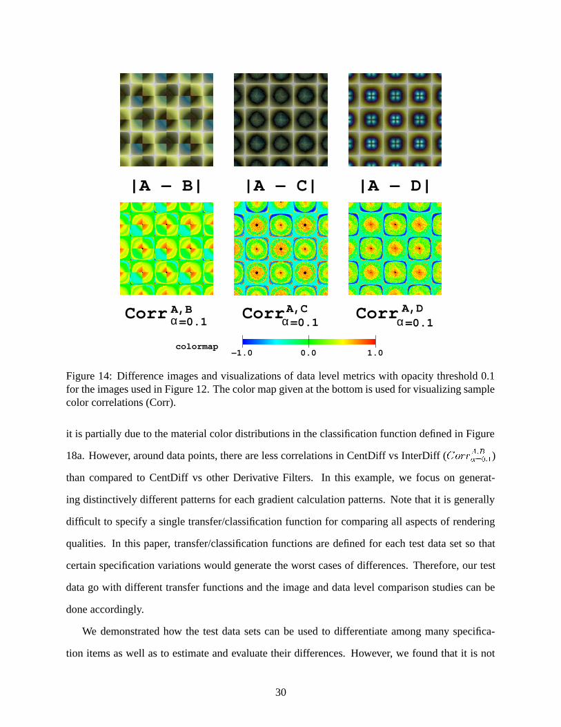
Figure 14 shows the difference images of Figure 12 and visualizations of the correlations be-

tween sample colors at each pixel. The difference images show that we generally have the largest

differences at the midpoints of the volume cells. CorrA;B�=0:1 is the correlation of two different

sample colors that have been generated by algorithm A and B along the viewing direction at each

pixel of Figure 12. Corresponding sample vectors are collected along the viewing direction until

both algorithms accumulate the threshold opacity 0.1 at each pixel. We can examine all the color

components but, in this example, we include visualizations for the green color component only.

Each difference image and data level metric shows a distinct pattern. The rendering differences of

CentDiff vs InterDiff, jA�Bj of Figure 14, is brighter overall compared to jA� Cj and jA�Dj.

Generally, the regions around data points have higher correlations than other locations, although

29

|A − B| |A − C| |A − D|

Corr A,Bα=0.1 CorrA,C

α=0.1Corr A,D

α=0.1

colormap−1.0 1.00.0

Figure 14: Difference images and visualizations of data level metrics with opacity threshold 0.1for the images used in Figure 12. The color map given at the bottom is used for visualizing samplecolor correlations (Corr).

it is partially due to the material color distributions in the classification function defined in Figure

18a. However, around data points, there are less correlations in CentDiff vs InterDiff (CorrA;B�=0:1)

than compared to CentDiff vs other Derivative Filters. In this example, we focus on generat-

ing distinctively different patterns for each gradient calculation patterns. Note that it is generally

difficult to specify a single transfer/classification function for comparing all aspects of rendering

qualities. In this paper, transfer/classification functions are defined for each test data set so that

certain specification variations would generate the worst cases of differences. Therefore, our test

data go with different transfer functions and the image and data level comparison studies can be

done accordingly.

We demonstrated how the test data sets can be used to differentiate among many specifica-

tion items as well as to estimate and evaluate their differences. However, we found that it is not

30

BIN

RB

|A − B|

|C − D|

A(C0,1EF) B(C0,3EF)

C(C0,1EF) D(C0,3EF)

Figure 15: Differences in gradient filters. We used both Binary (for A and B) and Region Boundary(for C and D) Surface classifications.

straight-forward to generate test cases that can differentiate certain algorithm variations. For exam-

ple, it is not easy to generate distinctively different images for algorithms using different gradient

calculation with derivative filters given by Moller [19]. The examples shown may seem to sug-

gest that simple datasets that highlight differences are easy to synthesize. The following example

is provided to give an indication to the contrary. Using a varying frequency checker board was

anticipated to be a good gradient error comparison because gradient filters have different sizes

and weights. Figure 15 shows the differences in some of the derivative filters. The size of the

entire data is 27 � 27 � 9 and it consists of 9 sub-data blocks. Each block of data is a 9 � 9 � 9

3DCheckerBoard. We gave different distance d and size of steps (step) to increment or decrement

the data values between minimum and maximum values. Figure 16 shows a one dimensional ex-

ample where d = 6 and two different step sizes. Details for each of the 9 sub-blocks of the data

31

d

d = 6step = 1

d

d = 6step = 2

H

L

Figure 16: Effects of changing step sizes in 3DCheckerBoard.

are specified in Figure 19 of the Appendix. These variations are attempts to increase differences

and generate distinctively different images for as many derivative filters as possible. However,

it does not generate more or better measures than the general qualitative differences that can be

assessed by Marschner and Lobb’s [16] data. For general quality comparisons of new algorithm

variations, some widely used standard test data (such as MRI brain) or specially designed data

[16, 20, 33] have been used. In some cases, these data sets can be superior differentiators between

algorithms. The advantage of our test suite is in differentiating specification items and performing

detailed comparison studies of algorithms using image and data level metrics. It includes assessing

differences in special or worst cases.

8 Summary

We discussed the list of important specifications for DVR algorithms. This list includes possibly

subtle variations that may often be ambiguous or even ignored in the published literature in the

field of volume rendering. We then presented two simple data sets that can be used for clearly

identifying variations in the algorithm specifications. The datasets generate differences that make

it simple to distinguish between rendering variants. This is a marked improvement over using test

data, where verisimilitude is the goal, because variations are only slight and may be overlooked.

We showed examples of the superiority of the checkerboard data over the commonly used MRI

brain, Hipip, and Marschner and Lobb data sets. The examples demonstrate the usage of the DVR

algorithm specification list and test data sets for in depth comparison studies via both image and

32

data level metrics. We also gave detailed specifications for our examples so that other researchers

may make more quantitative comparisons of different DVR methods. Our comparison study in-

cludes assessing differences in special and worst cases for the given algorithm variations. The new

datasets and metrics highlight differences between algorithms. In real datasets there will be subtle

differences, but it will be hard to say what is superior. These tools make it clear why the differ-

ences exist. It is up to the developer to determine the appropriate trade-offs for their applications

and datasets.

Most of the previous comparison methods use information from final rendered images only. We

overcome limitations of image level comparisons with our data level approach using intermediate

rendering information. We provide a list of rendering parameters and algorithm specifications

to guide comparison studies. We extend Williams and Uselton’s rendering parameter list with

algorithm specification items and provide guidance on how to compare algorithms. Real data is

often too complex to study algorithm variations with confidence. Most of the analytic test data sets

reported are often useful only for a limited feature of DVR algorithms. We provide simple and

easily reproducible test data sets, a checkerboard and a ramp, that can make clear differences in a

wide range of algorithm variations. With data level metrics, our test data sets make it possible to

perform detailed comparison studies.

Part of the results of this paper are to conclude that designing data to highlight differences is

difficult. And, we found that it was not possible in some cases to generate test data that resulted

in strong differences. In the beginning of this paper, we gave an overview of comparison studies

in which we use the specification list and test data sets from our earlier work [8, 9]. The tools pre-

sented here can be considered as another step towards an on-going research goal of providing more

standardized and objective comparison for DVR algorithms. We plan to extend and strengthen all

the steps involved in the comparison process including data level metrics, test data sets, and DVR

algorithm specifications.

33

9 Acknowledgements

We would like to thank Torsten Moller, the Client and Media Systems Laboratory of H.P. Labora-

tories, the members of the Advanced Visualization and Interactive Systems laboratory at UCSC,

and the anonymous reviewers for their feedback and suggestions. This project is supported in part

by DARPA grant N66001-97-8900, LLNL Agreement No. B347879 under DOE Contract No.

W-7405-ENG-48, NSF NPACI ACI-9619020, and NASA grant NCC2-5281.

A Appendix

In this section, we provide details of the rendering parameters and algorithm specifications used to

generate the images in the result section.

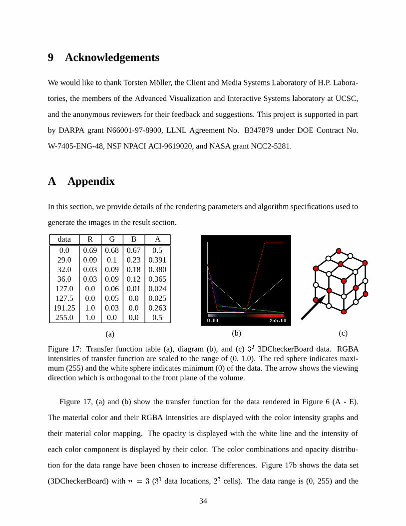
data R G B A

0.0 0.69 0.68 0.67 0.529.0 0.09 0.1 0.23 0.39132.0 0.03 0.09 0.18 0.38036.0 0.03 0.09 0.12 0.365

127.0 0.0 0.06 0.01 0.024127.5 0.0 0.05 0.0 0.025

191.25 1.0 0.03 0.0 0.263255.0 1.0 0.0 0.0 0.5

(a) (b) (c)

Figure 17: Transfer function table (a), diagram (b), and (c) 33 3DCheckerBoard data. RGBAintensities of transfer function are scaled to the range of (0, 1.0). The red sphere indicates maxi-mum (255) and the white sphere indicates minimum (0) of the data. The arrow shows the viewingdirection which is orthogonal to the front plane of the volume.

Figure 17, (a) and (b) show the transfer function for the data rendered in Figure 6 (A - E).

The material color and their RGBA intensities are displayed with the color intensity graphs and

their material color mapping. The opacity is displayed with the white line and the intensity of

each color component is displayed by their color. The color combinations and opacity distribu-

tion for the data range have been chosen to increase differences. Figure 17b shows the data set

(3DCheckerBoard) with n = 3 (33 data locations, 23 cells). The data range is (0, 255) and the

34

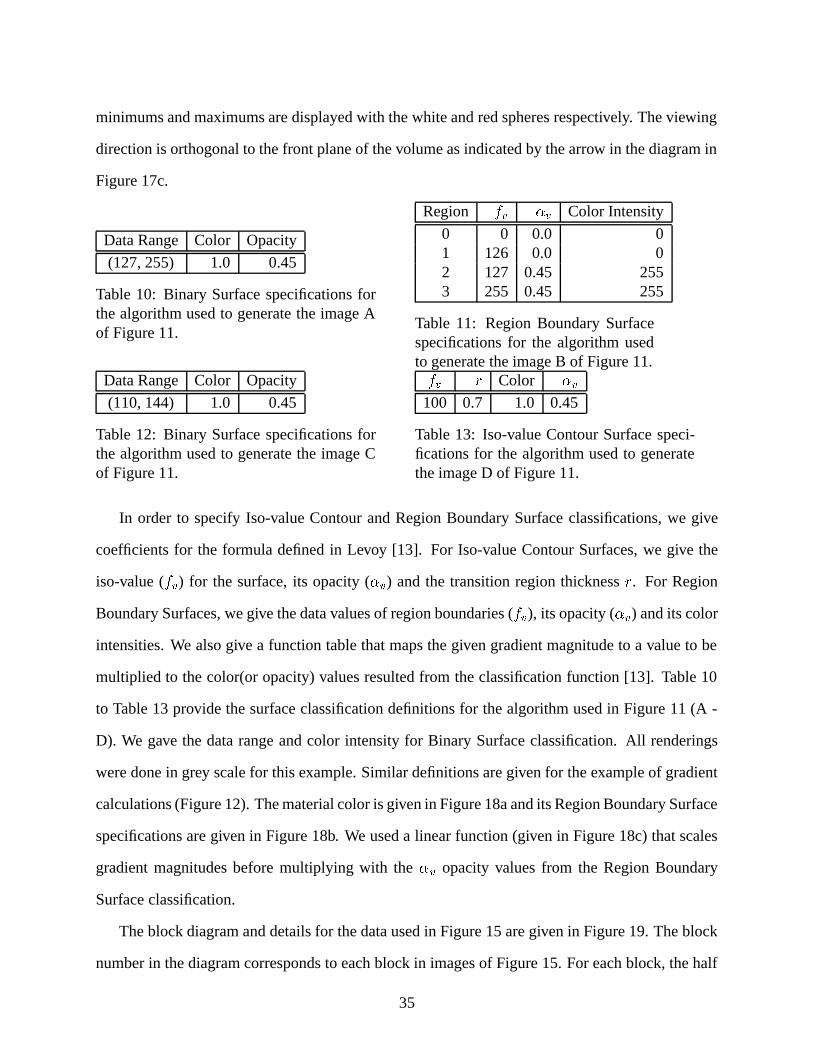
minimums and maximums are displayed with the white and red spheres respectively. The viewing

direction is orthogonal to the front plane of the volume as indicated by the arrow in the diagram in

Figure 17c.

Data Range Color Opacity

(127, 255) 1.0 0.45

Table 10: Binary Surface specifications forthe algorithm used to generate the image Aof Figure 11.

Region fv �v Color Intensity

0 0 0.0 01 126 0.0 02 127 0.45 2553 255 0.45 255

Table 11: Region Boundary Surfacespecifications for the algorithm usedto generate the image B of Figure 11.

Data Range Color Opacity

(110, 144) 1.0 0.45

Table 12: Binary Surface specifications forthe algorithm used to generate the image Cof Figure 11.

fv r Color �v

100 0.7 1.0 0.45

Table 13: Iso-value Contour Surface speci-fications for the algorithm used to generatethe image D of Figure 11.

In order to specify Iso-value Contour and Region Boundary Surface classifications, we give

coefficients for the formula defined in Levoy [13]. For Iso-value Contour Surfaces, we give the

iso-value (fv) for the surface, its opacity (�v) and the transition region thickness r. For Region

Boundary Surfaces, we give the data values of region boundaries (fv), its opacity (�v) and its color

intensities. We also give a function table that maps the given gradient magnitude to a value to be

multiplied to the color(or opacity) values resulted from the classification function [13]. Table 10

to Table 13 provide the surface classification definitions for the algorithm used in Figure 11 (A -

D). We gave the data range and color intensity for Binary Surface classification. All renderings

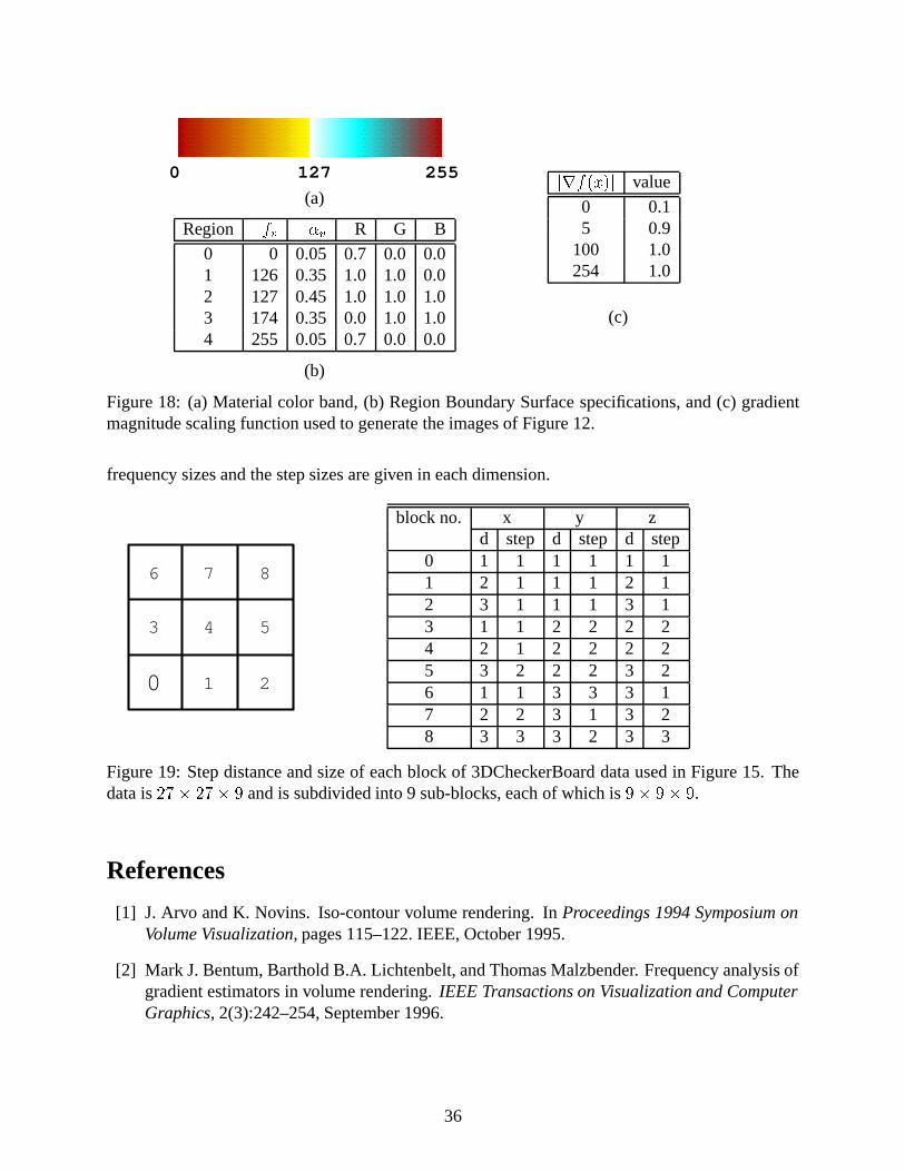
were done in grey scale for this example. Similar definitions are given for the example of gradient

calculations (Figure 12). The material color is given in Figure 18a and its Region Boundary Surface

specifications are given in Figure 18b. We used a linear function (given in Figure 18c) that scales

gradient magnitudes before multiplying with the �v opacity values from the Region Boundary

Surface classification.

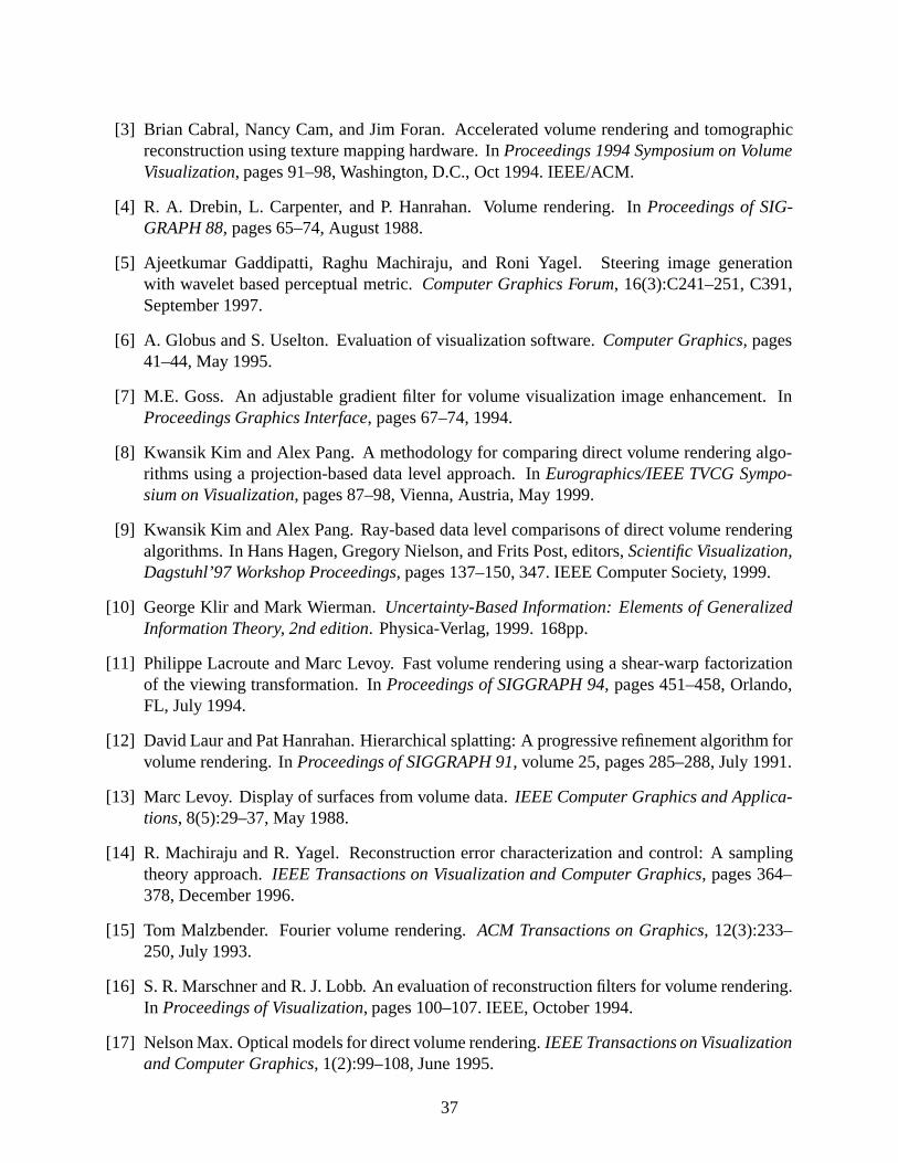
The block diagram and details for the data used in Figure 15 are given in Figure 19. The block

number in the diagram corresponds to each block in images of Figure 15. For each block, the half

35

0 255127

(a)

Region fv �v R G B

0 0 0.05 0.7 0.0 0.01 126 0.35 1.0 1.0 0.02 127 0.45 1.0 1.0 1.03 174 0.35 0.0 1.0 1.04 255 0.05 0.7 0.0 0.0

(b)

jrf(x)j value

0 0.15 0.9

100 1.0254 1.0

(c)

Figure 18: (a) Material color band, (b) Region Boundary Surface specifications, and (c) gradientmagnitude scaling function used to generate the images of Figure 12.

frequency sizes and the step sizes are given in each dimension.

0 1 2

3 4 5

6 7 8

block no. x y zd step d step d step

0 1 1 1 1 1 11 2 1 1 1 2 12 3 1 1 1 3 13 1 1 2 2 2 24 2 1 2 2 2 25 3 2 2 2 3 26 1 1 3 3 3 17 2 2 3 1 3 28 3 3 3 2 3 3

Figure 19: Step distance and size of each block of 3DCheckerBoard data used in Figure 15. Thedata is 27� 27� 9 and is subdivided into 9 sub-blocks, each of which is 9� 9� 9.

References

[1] J. Arvo and K. Novins. Iso-contour volume rendering. In Proceedings 1994 Symposium onVolume Visualization, pages 115–122. IEEE, October 1995.

[2] Mark J. Bentum, Barthold B.A. Lichtenbelt, and Thomas Malzbender. Frequency analysis ofgradient estimators in volume rendering. IEEE Transactions on Visualization and ComputerGraphics, 2(3):242–254, September 1996.

36

[3] Brian Cabral, Nancy Cam, and Jim Foran. Accelerated volume rendering and tomographicreconstruction using texture mapping hardware. In Proceedings 1994 Symposium on VolumeVisualization, pages 91–98, Washington, D.C., Oct 1994. IEEE/ACM.

[4] R. A. Drebin, L. Carpenter, and P. Hanrahan. Volume rendering. In Proceedings of SIG-GRAPH 88, pages 65–74, August 1988.

[5] Ajeetkumar Gaddipatti, Raghu Machiraju, and Roni Yagel. Steering image generationwith wavelet based perceptual metric. Computer Graphics Forum, 16(3):C241–251, C391,September 1997.

[6] A. Globus and S. Uselton. Evaluation of visualization software. Computer Graphics, pages41–44, May 1995.

[7] M.E. Goss. An adjustable gradient filter for volume visualization image enhancement. InProceedings Graphics Interface, pages 67–74, 1994.

[8] Kwansik Kim and Alex Pang. A methodology for comparing direct volume rendering algo-rithms using a projection-based data level approach. In Eurographics/IEEE TVCG Sympo-sium on Visualization, pages 87–98, Vienna, Austria, May 1999.

[9] Kwansik Kim and Alex Pang. Ray-based data level comparisons of direct volume renderingalgorithms. In Hans Hagen, Gregory Nielson, and Frits Post, editors, Scientific Visualization,Dagstuhl’97 Workshop Proceedings, pages 137–150, 347. IEEE Computer Society, 1999.

[10] George Klir and Mark Wierman. Uncertainty-Based Information: Elements of GeneralizedInformation Theory, 2nd edition. Physica-Verlag, 1999. 168pp.

[11] Philippe Lacroute and Marc Levoy. Fast volume rendering using a shear-warp factorizationof the viewing transformation. In Proceedings of SIGGRAPH 94, pages 451–458, Orlando,FL, July 1994.

[12] David Laur and Pat Hanrahan. Hierarchical splatting: A progressive refinement algorithm forvolume rendering. In Proceedings of SIGGRAPH 91, volume 25, pages 285–288, July 1991.

[13] Marc Levoy. Display of surfaces from volume data. IEEE Computer Graphics and Applica-tions, 8(5):29–37, May 1988.

[14] R. Machiraju and R. Yagel. Reconstruction error characterization and control: A samplingtheory approach. IEEE Transactions on Visualization and Computer Graphics, pages 364–378, December 1996.

[15] Tom Malzbender. Fourier volume rendering. ACM Transactions on Graphics, 12(3):233–250, July 1993.

[16] S. R. Marschner and R. J. Lobb. An evaluation of reconstruction filters for volume rendering.In Proceedings of Visualization, pages 100–107. IEEE, October 1994.

[17] Nelson Max. Optical models for direct volume rendering. IEEE Transactions on Visualizationand Computer Graphics, 1(2):99–108, June 1995.

37

[18] Torsten Moller, Raghu Machiraju, Klaus Muller, and Roni Yagel. A comparison of normalestimation schemes. In Proceedings of the IEEE Conference on Visualization 1997, pages19–26, October 1997.

[19] Torsten Moller, Klaus Muller, Yair Kurzion, Raghu Machiraju, and Roni Yagel. Design ofaccurate and smooth filters for function and derivative reconstruction. In Proceedings of the1998 Symposium on Volume Visualization, pages 143–151, October 1998.

[20] Ulrich Neumann. Volume Reconstruction and Parallel Rendering Algorithms: A ComparativeAnalysis. PhD thesis, UNC, Chapel Hill, 1993.

[21] Hans-Georg Pagendarm and Frits H. Post. Studies in comparative visualization of flow fea-tures. In G. Nielson, H. Hagen, and H. Muller, editors, Scientific Visualization: Overviews,Methodologies, Techniques, pages 211–227. IEEE Computer Society, 1997.

[22] A. Pang, C.M. Wittenbrink, and S. K. Lodha. Approaches to uncertainty visualization. TheVisual Computer, 13(8):370–390, 1997.

[23] Nivedita Sahasrabudhe, John E. West, Raghu Machiraju, and Mark Janus. Structured spatialdomain image and data comparison metrics. In Proceedings of Visualization 99, pages 97–104,515, 1999.

[24] U. Tiede, K.H. Hohne, M. Bomans, A. Pommert, M. Riemer, and G. Wiebecke. Surfacerendering: Investigation of medical 3D-rendering algorithms. IEEE Computer Graphics andApplications, 10(2):41–53, March 1990.

[25] Allen Van Gelder and Kwansik Kim. Direct volume rendering with shading via 3D textures.In ACM/IEEE Symposium on Volume Visualization, pages 22–30, San Francisco, CA, October1996.

[26] J. Terwisscha van Scheltinga, M.K. Bosma, J. Smit, and S. Lobregt. Image quality im-provements in volume rendering. In Lecture notes in computer science, (Fourth InternationalConference on Visualization in Biomedical Computing) VBC ’96, volume 1131, pages 87–92.Springer-Verlag, September 1996.

[27] L. Westover. Footprint evaluation for volume rendering. In Proceedings of SIGGRAPH 90,pages 367–376, August 1990.

[28] Lee A. Westover. Splatting: A Parallel, Feed-Forward Volume Rendering Algorithm. PhDthesis, University of North Carolina at Chapel Hill, 1991.

[29] Jane Wilhelms and Allen Van Gelder. A coherent projection approach for direct volumerendering. In Proceedings of SIGGRAPH 91, pages 275–284, 1991.

[30] Peter L. Williams and Nelson L. Max. A volume density optical model. In Proceedings of1992 Workshop on Volume Visualization, pages 61–68, Boston, October 1992.

[31] Peter L. Williams and Samuel P. Uselton. Metrics and generation specifications for comparingvolume-rendered images. The Journal of Visualization and Computer Animation, 10:159–178, 1999.

38

[32] Craig M. Wittenbrink, Thomas Malzbender, and Michael E. Goss. Opacity-weighted colorinterpolation for volume sampling. In Proceedings of the 1998 Symposium on Volume Visu-alization, pages 135–142, color plate page 177, October 1998. Also available as TechnicalReport, HPL-97-31R2, Hewlett-Packard Laboratories, Palo Alto, CA, Revised Apr. 1998.

[33] Craig M. Wittenbrink and A. K. Somani. Time and space optimal parallel volume renderingusing permutation warping. Journal of Parallel and Distributed Computing, 46(2):148–164,November 1997.

39