Export-led

growth? The case of Brazil

BACHELOR THESIS WITHIN: Economics

NUMBER OF CREDITS: 15 ECTS

PROGRAMME OF STUDY: International Economics

AUTHOR: Florian Schmidt

JÖNKÖPING May 2020

1

Bachelor Thesis in Economics

Title: Export-led growth? The case of Brazil

Author: Florian Schmidt

Tutor: Lina Bjerke

Date: 2020-05-18

Key terms: export-led growth hypothesis (ELGH); economic growth; neoclassical theory

of production; VECM; Granger Causality; Brazil

Abstract

With an ever-increasing globalising world, trade is of most importance for developing

countries to not fall behind and be outcompeted. Export-led growth theory states that one

of the key determinants for economic growth is exports. This thesis aims to analyse the

causal effects of exports on economic growth in the case of Brazil. Annual data from the

World Bank’s database for the years 1990-2018 has been used. The variables included

are GDP, exports, gross capital formation, FDI and labour force. This study puts the

export-led growth theory in a Vector Error Correction – Granger Causality framework.

As opposed to previous scholars’ findings, neither export-led growth nor growth-led

export could be determined for Brazil.

2

Table of Contents

Introduction ..................................................................................... 4

Economic characteristics of Brazil ........................................................................ 6

Theory ............................................................................................. 8

Neo-classical Growth Economic Theory ................................................................ 8

Export-led growth theory ..................................................................................... 9

Literature Review ........................................................................... 10

Export-led growth findings ................................................................................ 10

Growth-led exports findings ............................................................................... 12

Findings for bi-directional relationship between exports and economic

growth.. ............................................................................................................. 12

Findings for no causal relationship between exports and economic growth .......... 13

Hypothesis ...................................................................................... 15

Data….. ............................................................................................................. 15

Methodology ...................................................................................................... 17

Empirical model ................................................................................................ 18

Analysis and Results ....................................................................... 19

Discussion ....................................................................................... 34

Conclusions and limitations ............................................................. 36

Reference list .................................................................................. 38

Appendix ........................................................................................ 41

3

Figures

Figure 1 GDP Growth (Annual %) ..................................................................... 6

Figure 2 Exports as a share of GDP .................................................................... 7

Figure 3 Timeline chart GDP Brazil.................................................................. 20

Figure 4 Timeline chart Export Brazil ............................................................... 20

Figure 5 Timeline chart Capital Brazil .............................................................. 21

Figure 6 Timeline chart FDI Brazil ................................................................... 21

Figure 7 Timeline chart Labour force Brazil ...................................................... 22

Tables

Table 1 Spurious Regression ............................................................................ 23

Table 2 Augmented Dickey Fuller test .............................................................. 24

Table 3 Optimal lag length selection ................................................................. 25

Table 4 Johansen cointegration test ................................................................... 26

Table 5 Long-run VECM ................................................................................. 28

Table 6 Short-run VECM ................................................................................ 29

Table 10 Granger causality/ Wald test ............................................................... 31

Table 11 Pairwise Granger Causality Test ......................................................... 33

Table 12 Descriptive Statistics ......................................................................... 41

Table 13 Descriptive Statistics logged ............................................................... 41

Table 7 Breusch-Godfrey Autocorrelation test ................................................... 42

Table 8 Jarque-Bera Normality Test ................................................................. 43

Table 9 White's heteroskedasticity test .............................................................. 43

4

Introduction

The world is constantly evolving, and globalisation touches the economies of every

country in the world. One way of adjusting a country’s economy to the global market is

by trade. In this occurrence, export-led economic growth plays a major role in elevating

a country’s economy and contributing to the ascension on the global market (Temiz Dinç

& Gökmen, 2019). Export is not only a growth driver; it is also a factor which facilitates

inter-dependent relationships between the world’s countries. Export- led economic

growth has proven to be valuable for countries because it promotes inflow of foreign

exchange, increases production, promotes industrial and technological advancement,

creates new employment opportunities, and expands commercial volume. Furthermore,

export relaxes foreign exchange policies and increases efficiency through amplified

competition (Ehinomen, Daniel, 2012; Krasniqi, Topxhiu, 2017; Hatemi, Irandoust,

2000).

Having such a wide range of positive effects on a country’s economy, export promotion

strategies are preferred to other growth strategies by policy makers in developing

countries (Hatemi & Irandoust, 2000).

Over the last decades the Brazilian economy reached its peak between 2007 and 2012,

with a GDP growth at around 3,6 % per year. This period of growth was the result of both

domestic demand and international demand, and high Brazilian merchandise prices.

However, starting in late 2011, Brazilian growth decreased significantly, due to various

reasons such as: high taxes, inadequate infrastructure, and unsuccessful economic

policies, reaching an annual growth level of 0,9% per year (WTO, 2013).

Developing a sustainable economic growth and participating in multilateral trading

systems are two objectives of high importance to Brazil. To reach these objectives, Brazil

established a number of policies focusing on foreign trade, technology, and industry,

called ‘Plano Brasil Maior’ (Brazil Major Plan).

In addition to focusing on sustainable economic growth, Brazil is a founding member of

the Mercosur trade union, which formed in 1995 and is presently negotiating Free Trade

Agreements for its members. Mercosur was created with the aim of fortifying Brazil’s

policy of regional economic integration.

5

Furthermore, Brazil joined other developing countries, which were at a similar level of

economic development on their path of becoming developed countries and created

BRICS. BRICS is an economic organisation, which establishes trade relations for its

members, Brazil, Russia, India, China, and South Africa (WTO, 2013)

Having such a diverse range of policies and agreements promoting export, and being a

developing country, with a widely fluctuating GDP growth over the last decades, Brazil

represents the focus of this paper. Brazil was chosen as the subject of this thesis, based

on the findings of previous researchers, which state that export has a higher impact on

economic growth in a developing country and as Brazil is one of the biggest developing

countries in the world in terms of GDP.

This thesis wishes to examine the relationship between export and economic growth in

Brazil over the period 1990 to 2018, and therefore contribute to previous research by

adding recent findings. Therefore, this study aims to contribute to the current export-led

growth research by investigating if export causes economic growth, or if economic

growth causes export. Hence answering the research questions “Do exports cause

economic growth in Brazil?” and “Does economic growth cause exports in Brazil?”.

To conduct this analysis, the variable GDP is used as dependent variable in connection

with the independent variables export, foreign direct investment, and labour force. The

data ranges from the years 1990 to 2018 due to availability problems and this data will be

reviewed in a log-linear regression function.

This thesis is structured in eight chapters. In the introduction chapter the purpose and the

main research questions of the thesis have been presented. This paper continues with the

chapter presenting background information and country specific characteristics of Brazil,

in relation to export and economic growth. The third chapter briefly presents the core

theories of this study. The thesis continues with the fourth chapter, where previous

research conducted on export- led growth theory is reviewed and discussed. In the fifth

chapter the collected data and chosen methods of analysis are presented. The analysis of

the data and the results of this study are presented in the sixth chapter. The seventh chapter

consists of the discussion. Ultimately, the conclusions of the analysis and of this thesis

are stated in the eight chapter, which are followed by the reference list and appendices.

6

Economic characteristics of Brazil

In the years from 1990-1994 Brazil showed an impressive improvement of annual GDP

growth rates, from -3% to more than 5%. This initial growth, however, has stagnated and

even decreased reaching lows in 1998-1999; 2009 at about 0% and a major economic

activity contraction in 2015-2016 at around -3.5%. The 0% growth rate in 2009 is likely

caused by the global financial crisis, however followed by an impressive growth rate of

almost 8% as compared to other Latin American countries and countries in Europe and

Central Asia, which grew by only 4% and 2.5% respectively. From there on, Brazil’s

economy growth decreased and stagnated (Figure 1) (World Bank, 2020).

Not only economic growth of Brazil could be at a better stage, productivity growth and

infrastructure development need addressing as well, according to World Bank (2019). An

improper business environment and needless company support programs are additional

reasons for the low productivity of the country. Brazil can also be considered closed to

trade as compared to other countries with a low level of domestic competition.

Furthermore, the infrastructure lacks necessary investment, and those investments that do

exist are usually of poor quality (World Bank, 2019).

Figure 1 GDP Growth (Annual %)

Own creation with data received from World Bank (2020), where the GDP growth is

calculated in 2010 US-Dollar terms

7

Also, there is an increase in population aging, which causes the labour force to shrink,

which in turn leads to less productivity. To account for mentioned issues, Brazil’s

government must take actions, such as opening up for trade and reducing the costs of

doing business that occur from high barriers to entry in the market. Policies supporting

new technology and innovation should be the focus to increase productivity and help

boost Brazil’s international competition (World Bank, 2019).

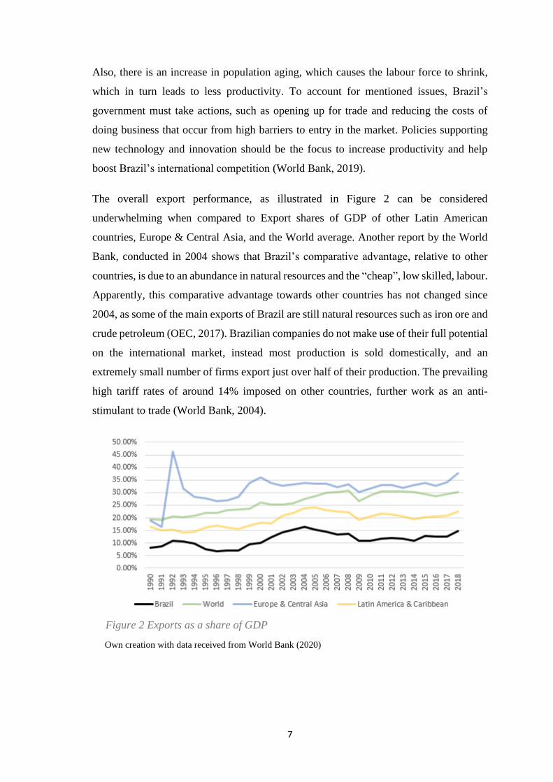
The overall export performance, as illustrated in Figure 2 can be considered

underwhelming when compared to Export shares of GDP of other Latin American

countries, Europe & Central Asia, and the World average. Another report by the World

Bank, conducted in 2004 shows that Brazil’s comparative advantage, relative to other

countries, is due to an abundance in natural resources and the “cheap”, low skilled, labour.

Apparently, this comparative advantage towards other countries has not changed since

2004, as some of the main exports of Brazil are still natural resources such as iron ore and

crude petroleum (OEC, 2017). Brazilian companies do not make use of their full potential

on the international market, instead most production is sold domestically, and an

extremely small number of firms export just over half of their production. The prevailing

high tariff rates of around 14% imposed on other countries, further work as an anti-

stimulant to trade (World Bank, 2004).

Figure 2 Exports as a share of GDP

Own creation with data received from World Bank (2020)

8

Theory

Classical economic growth theory found its roots mainly by Adam Smith and David

Ricardo. Another contributor to the classical growth theory was Marquis de Mirabeau

who connects economic growth and labour force, by stating that an increase in productive

labour causes an increase in wealth (here referred to as economic growth). Smith’s view

was that the process of economic growth is dependent on the productivity of labour and

capital accumulation and the driving forces for economic growth were endogenous. By

having the labour force divided in “productive” and “unproductive” labour, he could

explain output growth, where “productive” labour had a positive impact on the economy

and “unproductive” labour had a negative impact. The exogenous view on the economic

growth was mainly established by David Ricardo. Ricardo’s concept of economic growth

was explained as, with increasing capital and increasing labour ceteris paribus, profits

would not be increasing as land and machinery would wear out eventually causing

diminishing returns to scale. According to Ricardo, a comparative advantage, known as

a technological advantage and increasing exports would lead to economic growth,

assuming barriers to trade were held low (Eltis, 2000).

Neo-classical Growth Economic Theory

As opposed to the classical economic theory, neo-classical economic theory puts supply

and demand in the focus for production. This “new” economic theory states that prices

are determined through the individuals’ demand and their willingness to pay (utility), as

compared to the classical view stating that prices of goods are determined by the

production costs plus the labour costs. Furthermore, the neo-classical view was based on

the exchange of goods, rather than on their production (classical view), which further

supports the “free market approach” (Thirlwall, 2002).

The Solow Growth Model (or Solow-Swan model) (Solow, 1956) is a model developed

during the neo-classical economic era and it describes the long run economic growth rates

based on the variables capital, labour, and technology. In this model, technology is the

driving factor for growth, else the economy would stagnate due to diminishing marginal

returns. The effect of technology on growth can be explained as an increase in technology

causing the labour productivity to increase, which in turn leads to enhanced economic

growth.

9

Export-led growth theory

The export-led growth theory is based on the views of classical economic theory and neo-

classical economic theory. According to this theory, export is the main determinant for

economic growth. This can be explained as an increase in exports leading to an increase

in employment of the export-based industry and this increase leads to a higher

productivity, which in turn leads to an increase in economic growth. The export-led

growth theory has mainly been discussed in the years around the change of the

millennium, therefore one could argue that this growth theory has become obsolete.

However, there are still scholars investigating the effect exports have on economic

growth, hence this argument is not fully valid. There are various groups of export-led

growth; scholars having found a causal effect of exports on economic growth; the findings

of a causal effect of economic growth on exports; a feedback causal relationship, meaning

a bidirectional causal relationship, between exports and economic growth; and the

scholars who have found no support at all for a causal relationship of export on economic

growth or economic growth on exports.

Built on the previously discussed theories, this thesis aims to investigate the applicability

of these theories nowadays, in the case of Brazil. In doing so, this thesis moves on with

presenting the findings of previous researchers on the subject of export-led growth.

10

Literature Review

The relation between export and economic growth has been the core of many empirical

studies. The economic literature has been largely enriched, during the recent years by

authors who have conducted research on these topics (Mangir, 2012).

Theories such as Adam Smith’s and David Ricardo’s Classical Economic Theory, the

Neo- Classical Economic Growth Theory and the Export Led Growth theory had a great

impact on the general acceptance of the positive impact of trade and export on economic

growth (Mangir, 2012).

Although the theoretical views on this matter provided valuable information regarding

export and economic growth, an empirical analysis of peer-reviewed articles and research

papers, will provide a deeper and more complete understanding on the issue of export and

economic growth. This is what this chapter wishes to do. This subject is a highly debated

topic within economics, yet a controversial one. In this paper the views of this matter

have been divided into the following 4 categories: first category, where scholars have

concluded that export growth is the reason for economic growth; second category, where

researchers concluded economic growth to be the reason for export growth; third

category, where scholars found that export growth is the reason for economic growth and

economic growth is the reason for export growth and the findings of the fourth category,

where neither export growth nor economic growth are the reasons for one another.

Export-led growth findings

Ram (1985) studies the role of exports on economic growth, on a sample of 73 low income

and middle-income countries. The article debuts with analysing previous research papers

on the same subject, conducted by various authors, such as: Michaely, Balassa, Krueger,

and Tyler.

Ram (1985) states that the aim of his paper is not to oppose the findings of the previous

researchers, but to investigate if they are applicable to a larger sample of countries. The

previous research he has studied have concluded that there is a relationship between

export and economic growth. Furthermore, Ram has also divided the data into two

periods: 1960 to 1970 and 1970 to 1977, with the aim of arbitrating if the importance of

exports increased from a decade, to another. In doing so, the author has used the method

11

of regression, based on the aggregate production function model, with labor input, input

of capital and exports as variables (Ram, 1985).

On one hand, the author has concluded that export performance is significant for

economic growth, statement which further enhances the work of previous researchers. On

the other hand, his hypothesis that the importance of exports has amplified during the

1970 was proven to be right. The last conclusion reached in his study is that in low income

countries, the impact of export on economic growth is small, in comparison to the middle-

income countries, where the impact of export on economic growth is high (Ram, 1985).

Another study that emphasized the positive effect of export on economic growth is

‘Exports, policy choices, and economic growth in developing countries after the 1983 oil

shock’ (1985) by Bela Balassa. The paper aimed to examine the effects of export on

economic growth during the period after the 1973 of oil shock, on 43 low developed

countries (LDC), (Balassa, 1985).

The paper was based on previous research findings, which concluded that export have a

positive impact on economic growth. However, the author wished to test if this statement

will be applicable to a period where an external shock, such as the oil shock, could affect

the economic situation. Therefore, the article studied the period from 1973 to 1979.

Bela Balassa (1984) concluded that the rate of growth of exports had a major effect on

the economic growth. Furthermore, the author has observed that the numerical magnitude

of the effect considerably increased, compared to the period preceding the oil shock,

which was studied in a previous paper.

In the study ‘Rapid Growth in NICs in Asia: Tests of New Growth Theory for Korea’,

Jati K. Sengupta (1991) investigated through empirical tests the Growth Theory, on the

Asian countries, with focus on the case of Korea. The author has argued his choice of

conducting the study on Korea, based on the work of previous researches, which

concluded that the national policies of the country showed openness to trade more

powerfully than other Asian countries (Sengupta, 1991).

The author used an Ordinary Least Square method for the specified production function,

with the logged variables of GDP, export, labour, and capital, on a data set from 1967 to

1986.

12

The results of the study support the neo-classical growth theory and the author’s

hypothesis that state policies which promote export, have contributed to Korea’s

economic growth.

Growth-led exports findings

The studies analysed in the previous category have shown that export have a positive

impact on economic growth. While this body of literature is of high relevance for this

paper, there are also authors which state the opposite, that Economic growth has an impact

on exports.

Research of high importance to this subject, is the one conducted by Shan and Tian

(1998). The authors have studied the causality between export and economic growth on

the case of Shanghai. By using the Granger no causality procedure in a vector

autoregression model Shan and Tian (1998) have tested the export-led growth hypothesis,

on monthly data, over the period 1990 to 1996. Their results conclude that there is a one-

way causality between GDP and exports in Shanghai. However, another critical finding

of their research is that economic growth affects exports, if the internal production grows

at a higher rate than the internal demand (Shan, &Tian, 1998).

Findings for bi-directional relationship between exports and economic

growth

Ghartey (1993) has based his research of the countries Japan, US, and Taiwan on the

causal relationship that export growth causes economic growth of the countries. By the

use of the Wald – and the likelihood test, he analysed the variables exports, GNP, capital

stock and the terms of trade for stationarity. Yearly data from 1960-1990 was used for the

US and Taiwan, for Japan the data available ranged from 1955 – 1991. Furthermore, he

makes use of the Granger-causality test to find the direction of causation for the given

variables. Ghartey (1993) concludes the causal relation that economic growth has on

exports for the US, while he finds the opposite for Taiwan. Japan proves to have feedback

causal relationship, meaning there is a causal relationship of exports on economic growth

and economic growth on exports.

Sharma and Dhakal (1994) have also found evidence for a causal relationship between

export and economic growth in both directions by analysing 30 developing countries. The

authors used a Perron test to account for possible serial correlation and time dependent

13

heteroscedasticity on the variables output, capital, labour and real export and making sure

the variables are stationary by logging them and taking the first- or second difference (if

necessary) for each country. With the help of F-statistics, the authors found support of a

unidirectional relationship, and their primary hypothesis, between export and economic

growth for 6 countries. For 8 countries they found support of an opposite relationship,

meaning economic growth affecting exports, while a feedback relationship, meaning

exports cause economic growth and economic growth causes exports, has been found for

5 countries. As a special case, the authors found out that there was no causal relationship

between export and economic growth for South Korea, which was assumed to derive its

growth from an export orientation (Sharma & Dhakal, 1994).

Furthermore, another study investigating the bidirectional causality between export and

economic growth, was conducted by Jordan Shan and Fiona Sun (1998) with time series

data from China. The authors have applied the Granger causality test in a VAR system

with industrial output as dependent variable and capital expenditure, labour force, energy

consumption, exports and imports as independent variables, on monthly data between

1978 and 1996 (Shan & Sun, 1998).

Shan and Sun (1998) have reached results which display a bidirectional causality between

exports and economic Growth in China, during the studied period.

Findings for no causal relationship between exports and economic

growth

The fourth and final category of the current literature review is comprised of research

papers which argue that there is no causal relationship between export and economic

growth.

One of the articles supporting this statement is ‘Export performance and economic

development: an empirical analysis’ by Yaghmaian and Ghorashi (1995). The authors

have challenged the findings of previous literature, which supports the neo classical view

on the export-led growth theory. In doing so, two sets of growth regressions were applied

on data from 30 developing countries, during the period 1980-1990.

The research paper was based on the hypothesis that economic growth and exports growth

are determined by prior compound economic process, which leads to major structural

changes and economic development. The results of the regression support their

14

hypothesis and do not support the export-led economic growth theory. The authors

concluded that both, export, and economic growth are the outcome of development and

technological changes (Yaghmaian & Ghorashi, 1995).

In the paper ‘Exports and economic growth’ by Anwer, M. and Sampath, R.K. (1997) the

authors challenge the export-led growth theory, arguing that previous research was

conducted on data sets which are not homogenous, because of the great differences

between demographic structures and the economy of every country.

The study was conducted on a sample of 96 countries, during a period of 32 years, from

1960 to 1992. The applied method was a regression based on Granger’s causality

approach. The authors have used the Augmented Dickey Fuller test, in order to ensure

stationarity of the variables.

Even though the analysis the authors revealed evidence of export growth influencing

economic growth in nine of the studied countries, the paper concludes that results are

different for every country, statement which supports their hypothesis.

While this extensive amount of literature, provided great information and insight on the

export-led growth theory in various countries, it can be concluded that most of the

research was conducted for periods between 1960 and 1990.

Lastly, the work of previous researchers provided inspiration for choosing the variables

and the analysis methods of this thesis, which will be further detailed in the methodology

chapter.

15

Hypothesis

To test for what has been researched in previous sections and to answer initially stated

research questions “Do exports cause economic growth in Brazil?” and “Does economic

growth cause exports in Brazil?”, four hypothesis statements are made. These hypotheses

can be tested in an econometrical framework (Gujarati, 2003), using empirical data of

Brazil.

Hypothesis 1

H0: Export growth does not cause economic growth in Brazil

H1: Export growth does cause economic growth in Brazil

Hypothesis 2

H0: Economic growth does not cause export growth in Brazil

H1: Economic growth does cause export growth in Brazil

Data

The variables specified in this thesis work cover the time period from 1990 to 2018 for

the country Brazil. It is annual data retrieved from the World Bank’s database, as

quarterly data was not available. Starting with the dependent variable to observe export-

led economic growth for the case of Brazil, this thesis analyses data on the gross domestic

product (GDP) in terms of current US-Dollar. The independent variables are as follows,

exports of goods and services, also in terms of current US-Dollar, gross capital formation

in current US-Dollar, foreign direct investments (FDI), measured as net inflows in terms

of current US-Dollar and the total labour force.

All scholars, that have been working with the export-led growth theory have included

variables to represent the output of an economy (such as GDP or GNP) and exports as

their main variables to analyse in their econometric model. Very often the growth rates

of given variables, by taking the logarithm, are used. Previous studies, however, differ in

what other variables to include in their empirical model, while most scholars have only

included an output variable and an export variable (Ghartey, 1993; Hatemi-J & Irandoust,

2000; Maneschiöld, 2008; Mangir, 2012; Gokmenoglu, Sehnaz & Taspinar, 2015). Other

16

scholars such as Ram 1985 and Yaghmaian & Ghorashi 1995 and Malhotra & Kumari,

2016 include variables representing capital and labour or population. Many studies on

developing countries (Shan & Tian, 1998; Krasniqi & Topxhiu, 2017; Hagemejer &

Muck, 2019) have used a variable for investment, as a proxy for change in technology, in

the model. This is because investment, especially foreign direct investment, can be seen

as means to improve technology for developing countries (Lensink & Morrisey, 2006).

The variables included in the model, in order to examine whether or not there is an effect

of export growth on economic (GDP) growth, are as follows.

Gross domestic product (GDP)

Gross domestic product is the dependent variable in this study, describing economic

growth. It includes the market value of all Brazilian final goods and services produced in

the time period from 1990-2018. For consistency, it is denoted in current US Dollar.

Exports (EX)

Exports is one of the independent variables in this study. It is the variable with highest

priority, alongside GDP, as it primarily revolves around the research question. Here, it is

denoted as exports of goods and services in US Dollar. It is expected to have a positive

impact on economic growth (GDP) according to economists such as David Ricardo,

however studies have shown varying results.

Gross capital formation (CAP)

Gross capital formation is another independent variable included. It covers the addition

of capital goods for firm production and is supposed to increase productivity. It is stated

in current US Dollar and serves as proxy for capital in the production function.

Furthermore, this variable is expected to have a positive impact on economic growth,

since an increase in productivity is associated with an increase in economic growth.

Foreign direct investment (FDI)

Foreign direct investment is also an independent variable to describe the net inflows of

foreign direct investment in current US Dollar into Brazil. It serves as a control variable

and is expected to have a positive impact on economic growth, as an increase in FDI can

be linked to an improvement of technology (Lensink & Morrisey, 2006). This can be said

17

for developing countries; however, it also highly depends on government decisions and

policy.

Labour force (LF)

The independent variable labour force is denoted in absolute terms and is a control

variable to explain changes in GDP more accurately. An increase in total labour force is

directly linked with an increase in GDP (or economic growth), hence it is expected to

have a positive impact on the variable GDP.

For further details about the variables, Table 12 and 13 in the appendix show the

descriptive statistics.

Methodology

This research paper analyses the potential causal effects of exports on economic growth

in Brazil. First, the time path structure of the variables is observed. Then, a spurious

regression is run on purpose, to show non-stationarity of the variables. Afterwards, an

Augmented Dickey Fuller (ADF) (Dickey & Fuller, 1981) unit root is conducted to

support the results of the spurious regression and test the variables for their stationarity at

level and at their first difference value. Furthermore, the optimal lag length for the model

is determined using the VAR lag length criterion, provided by EViews, where the

Schwartz Information Criterion (SIC) selects the appropriate lag length. Having selected

the optimal lag length, the Johansen Cointegration test (Johansen & Juselius, 1990) is run

to check for cointegration between the variables. After checking for cointegration the

Vector Error Correction Model (VECM) (Engle & Granger, 1987) is constructed, similar

to works from Ehinomen & Daniel, 2012 and Malhotra & Kumari, 2016. Various validity

tests are run thereafter, such as the Breusch-Godfrey autocorrelation test, the Jarque-Bera

normality test and White’s heteroskedasticity test. To check the direction of causality,

common procedure is to run a Granger causality/ Wald test and/ or a Pairwise Granger

causality test. In this research paper both tests are used, for robustness.

18

Empirical model

The empirical model takes the form of a production function and is specified as:

𝐺𝐷𝑃 = 𝑓(𝐸𝑥, 𝐶𝑎𝑝, 𝐹𝐷𝐼, 𝐿𝐹) (1)

The econometric form equation can be written as follows

𝐺𝐷𝑃𝑡 = 𝛽0 + 𝛽1𝐸𝑥𝑡 + 𝛽2𝐶𝑎𝑝𝑡 + 𝛽3𝐹𝐷𝐼𝑡 + 𝛽4𝐿𝐹𝑡 + 𝜀𝑡 (2)

Where 𝑡 = 1990, 1991, … , 2018

This model is denoted as a Log-log model, since all the variables are of logarithmic form,

making it easier to transform the data to stationary data. In equation (2) 𝐺𝐷𝑃𝑡 stands for

the time series data of Brazil’s gross domestic product. 𝛽0 is the constant term, and 𝛽1,

𝛽2, 𝛽3 and 𝛽4 are the respective coefficients for the variables 𝐸𝑥𝑡 = exports, 𝐶𝑎𝑝𝑡 = gross

capital formation, 𝐹𝐷𝐼𝑡 = foreign direct investment and 𝐿𝐹𝑡 = labor force. The error term

for the specified time period is denoted as 𝜀𝑡.

19

Analysis and Results

This paper aims to analyse previously described variables in order to answer the research

questions “Do exports cause economic growth?” and “Does economic growth cause

exports?” through conducting various tests in the statistical software EViews. First, it will

show the time structure of the variables GDP, exports, capital, FDI and labour force.

Second, a spurious regression will be run to evaluate non-stationarity of the variables in

their level form. To support the outcome of the spurious regression, an Augmented

Dickey Fuller test will be conducted to confirm the variables’ stationarity at first

difference. Third, the optimal number of lags will be selected using the vector

autoregressive lag length model. Fourth, the Johansen cointegration test will be

performed to ensure cointegration of the variables. Fifth, the vector error correction model

will be run, creating the long-run and the short-run output. Sixth, the vector error

correction model will be checked for its validity using the Breusch-Godfrey

autocorrelation test, the Jarque-Bera normality test and the White’s heteroskedasticity

test. And finally, the Granger Causality/ Wald test and the Pairwise Granger Causality

test will be run simultaneously to find out the causal relationship of exports on economic

growth, or economic growth on exports, or a feedback relationship, or a non-existent

causal relationship and to give robustness to the results.

Time paths

First of all, the time paths of all variables will be determined. This is done by looking at

the data graphs (Figure 3-7) of every individual logged variable.

The time paths of the GDP and the exports show a similar pattern in the years 2002 –

2017. This is good, as it can indicate that exports and GDP presume to be affected by

similar factors. But by looking at the time paths only, we cannot make any conclusions

for causal relationships. For the years 1998 – 2002 however, there is a decrease of GDP

which is matched with an increase of exports. The low value for GDP in the year 2002,

depicted in Figure 3, might be due to the South American crisis and the current account

deficit in 2002 (IMF, 2007). The peak in GDP in the years 2011-2012 is likely caused by

Brazil’s boom just after the financial crisis in 2009. The capital time series (Figure 5)

shows a very similar pattern to the GDP series with increasing and decreasing trends in

the same years. The FDI time series (Figure 6) shows an increasing trend between 1993

20

and 1998, a small decreasing trend is also observable from the end of the year 2000 until

2003. Afterwards, the time series seems to be increasing with a fluctuating pattern. The

labour force time series (Figure 7) indicates a constant increase, along a trend, over the

years 1990-2018. An overall increasing pattern of all time series can be observed.

Data retrieved from World Bank (2020)

Figure 3 Timeline chart GDP Brazil

Data retrieved from World Bank (2020)

Figure 4 Timeline chart Export Brazil

21

Figure 5 Timeline chart Capital Brazil

Figure 6 Timeline chart FDI Brazil

Data retrieved from World Bank (2020)

Data retrieved from World Bank (2020)

22

Having analysed the time paths of the various logged variables, the next step is to move

on and determine their stationarity.

Spurious regression

One way to check if the variables in their logged forms are non-stationary, is by

performing an Ordinary Least Squares (OLS) regression on the dependent variable GDP,

with export, capital, FDI and labour force as independent variables. The following output,

as shown in Table 1, is a case of a spurious regression. A spurious regression falsely

shows a relationship between non-stationary, independent variables. The Durbin-Watson

statistic is a measure for autocorrelation of a model, and it ranges from 0 to 4. The R-

squared value ranges from 0 to 1 and it measures, in percentages, how much the variation

of the dependent variable is explained by the independent variables. As a rule of thumb,

one can say that a regression is spurious when the Durbin-Watson statistic (0.79) is

smaller than the R-squared value (0.98). Ideally, the value for the Durbin-Watson statistic

should be close to 2, if it is close to 0 or 4 it is an indication that the model suffers from

serial correlation. The high R-squared value of almost 1 can also be an indication for a

spurious regression, as such high values of fit are rare. However, since a spurious

regression provides a misleading output it should not be interpreted (Ventosa-Santaulària,

2009).

Figure 7 Timeline chart Labour force Brazil

Data retrieved from World Bank (2020)

23

Table 1 Spurious Regression

Variable Coefficient Std. Error t-Statistic Prob.

C -6.67 11.09 -0.60 0.55

LN_EX -0.06 0.23 -0.27 0.79

LN_CAP 0.84 0.14 5.94 0.00

LN_FDI 0.01 0.04 0.22 0.83

LN_LF 0.76 0.78 0.97 0.34

R-squared 0.98 Mean dependent var 27.66

Adjusted R-

squared 0.98 S.D. dependent var 0.62

S.E. of regression 0.09 Akaike info criterion -1.82

Sum squared

resid 0.20 Schwarz criterion -1.58

Log likelihood 31.34 Hannan-Quinn criter. -1.74

F-statistic 326.00 Durbin-Watson stat 0.79

Prob(F-statistic) 0.00

Augmented Dickey Fuller test

Even though the spurious regression cannot be interpreted, it has shown that the

independent variables are non-stationary, hence an Augmented Dickey Fuller test (ADF)

is performed to account for the problem of non-stationary variables. This test is based on

the null hypothesis of an existing unit-root. Rejecting this null hypothesis means that there

is no unit root problem and the variable is stationary and accepting the null hypothesis

means that there is a unit root problem and the variable is non-stationary. The exogenous

term describes the time path of the variable, e.g. “constant” means there is an increasing

trend, and “Constant, trend” means that there is an increasing trend around a mean. Table

2 shows the ADF test results, where the lag length was automatically selected by the

Schwartz Information Criterion (SIC). First, the ADF test is run on level data to show the

variables’ non-stationarity. The results of the ADF test show indeed that the variables in

their level form have been non-stationary. Because, for all the level variables, the null

hypothesis of an existence of a unit root cannot be rejected, as their p-values exceed the

selected significance level of 0.05. Then, the first difference of all variables is taken

(denoted by d( )), and since the p-values are lower than the specified significance level of

0.05, the null hypothesis of an existing unit root can be safely rejected. Hence, the

variables are stationary at first difference.

24

Table 2 Augmented Dickey Fuller test

Variable t-

statistic p-value Exogenous Lags Stationarity

GDP -1.05 0.72 Constant 0 Non-

Stationary

Ex -0.95 0.76 Constant 0 Non-

Stationary

Cap -1.20 0.66 Constant 0 Non-

Stationary

FDI -2.08 0.26 Constant 0 Non-

Stationary

LF -0.67 0.97 Constant,

trend 0

Non-

Stationary

d(GDP) -4.40 0.00 Constant 0 Stationary

d(Ex) -5.48 0.00 Constant 0 Stationary

d(Cap) -4.74 0.00 None 0 Stationary

d(FDI) -4.74 0.00 None 0 Stationary

d(LF) -5.38 0.00 Constant,

trend 0 Stationary

25

Optimal lag length selection

Having analysed the stationarity of the variables, one can now determine the optimal lag

length to choose the number of lags that should be included for the Johansen

Cointegration test and for the Vector Error Correction model. The optimal lag length is

determined in Table 3, and the Schwarz Information Criterion (here, SC), used for

consistency, provides an optimal lag length of 2, denoted by the asterisk next to the

number -10.28. This optimal lag length holds true for the whole model.

Table 3 Optimal lag length selection

Lag LogL LR FPE AIC SC HQ

0 38.54 NA 0.00 -2.48 -2.24 -2.41

1 182.46 223.87 0.00 -11.29 -9.85 -10.87

2 229.35 55.58* 0.00* -12.92* -10.28* -12.13*

Note: * indicates lag order selected by the criterion

LR: sequential modified LR test statistic (each test at 5% level)

FPE: Final prediction error

AIC: Akaike information criterion

SC: Schwarz information criterion

HQ: Hannan-Quinn information criterion

26

Johansen cointegration test

The next step is to run the Johansen cointegration test (Johansen & Juselius, 1990) on the

variables in their level form (no first difference) and check for cointegration of the

variables. Table 4 shows the output for the Johansen Cointegration test. To clarify,

“None” meaning that there is no cointegration among the 5 variables, “At most 1”

meaning that there is no cointegration for at most 1 co-integrated equation and “At most

2” meaning that there is no cointegration for at most 2 co-integrated equations. The null

hypothesis of no co-integration is rejected by both tests (Trace and Maximum Eigenvalue)

for none, at most 1 and at most 2 cointegration equations, due to the p-values that are

lower than the significance level of 0.05. Furthermore, the Trace test and the Maximum

Eigenvalue test both show that there are 3 co-integrating equations at the 0.05 significance

level, as we cannot reject that there is no cointegration for at most 3 cointegrating

equations since the p-value for “at most 3” is greater than the significance level.

Table 4 Johansen cointegration test

Unrestricted Cointegration Rank Test (Trace)

Hypothesized

No. of CE(s) Eigenvalue

Trace

Statistic

5% Critical

Value Prob.**

None * 0.93 151.69 69.82 0.00

At most 1 * 0.78 79.49 47.86 0.00

At most 2 * 0.64 39.02 29.80 0.00

At most 3 0.28 11.68 15.49 0.17

At most 4 0.10 2.79 3.84 0.10

Note: Trace test indicates 3 cointegrating equations at the 0.05 level

* denotes rejection of the hypothesis at the 0.05 level **MacKinnon-Haug-Michelis (1999) p-values

Unrestricted Cointegration Rank Test (Maximum Eigenvalue)

Hypothesized

No. of CE(s) Eigenvalue

Max-Eigen

Statistic

5% Critical

Value Prob.**

None * 0.93 72.20 33.88 0.00

At most 1 * 0.78 40.46 27.58 0.00

At most 2 * 0.64 27.35 21.13 0.01

At most 3 0.28 8.89 14.26 0.30

At most 4 0.10 2.79 3.84 0.10

Note: Max-eigenvalue test indicates 3 cointegrating equations at the 0.05

level

* denotes rejection of the hypothesis at the 0.05 level **MacKinnon-Haug-Michelis (1999) p-values

27

Vector Error Correction Model

Since the Johansen Cointegration test provided the result of cointegration between the

variables, it is possible to continue by estimating the Vector Error Correction Model

(VECM) to find out how the variables behave in the long-run and in the short-run. As

cointegration implies the existence of a long-run relationship of the variables. The lags

for the VECM are selected based on the optimal lag length defined in Table 3 minus 1.

This provides the lag selection of 2-1 = 1 lag.

Long-run VECM

The long run VECM is specified as follows:

𝐸𝐶𝑇𝑡−1 = [𝑌𝑡−1 − 𝑛𝑗𝑋𝑡−1 − 𝜁𝑚 + 𝑅𝑡−1] (3)

𝐸𝐶𝑇𝑡−1 = 1.000𝑙𝑛𝐺𝐷𝑃𝑡−1 + 3.77𝑙𝑛𝐸𝑋𝑡−1 − 3.15𝑙𝑛𝐶𝐴𝑃𝑡−1 + 0.69𝑙𝑛𝐹𝐷𝐼𝑡−1 −

14.62𝑙𝑛𝐿𝐹𝑡−1 + 208.54 (4)

Table 5 shows the long run cointegrating output of the VECM. The long-run equilibrium

is based on level data. Now, the long run VECM is to be interpreted. First, it is notable

that all coefficients are significant at the 1% level, as determined by the respective t-

values shown in Table 5, since the absolute values exceed the 95% critical level of 2.473.

This critical level is based on the t-distribution and 27 degrees of freedom. Therefore, the

coefficient of the variable ln_EX of 3.77 indicates that a one percent change of the

variable export causes the variable GDP to increase by around 3.77% in the long run,

ceteris paribus (keeping the other variables constant). Looking at the coefficient of the

variable ln_CAP -3.15, it means that one percent change in the variable capital causes the

dependent variable GDP to decrease by around 3.15% in the long run, ceteris paribus.

Furthermore, looking at the coefficient for the variable ln_FDI 0.69, one can say that a

one percent change in the variable FDI causes the variable GDP to increase by around

0.69% in the long run, ceteris paribus. Lastly, the coefficient for the variable ln_LF of -

14.62, means that a one percent change in the variable labour force causes the variable

GDP to decrease by approximately 14.62%.

In the long run the VECM predicts that export has a positive effect on GDP. Capital has

a negative effect on GDP, FDI has a positive effect on GDP and lastly, labour force has

28

a negative effect on GDP. As mentioned previously, these results are significant at a 95%

confidence interval.

Table 5 Long-run VECM

Cointegrating

Eq: CointEq1 St. Error T-statistics

LN_GDP(-1) 1

LN_EX(-1) 3.77 -0.28 13.35

LN_CAP(-1) -3.15 -0.18 -17.25

LN_FDI(-1) 0.69 -0.06 12.21

LN_LF(-1) -14.62 -0.99 -14.77

C 208.54

Note: (-1) represents number of lags

Short-run VECM

The short run VECM is specified as:

∆𝑙𝑛𝐺𝐷𝑃𝑡 = −0.19𝐸𝐶𝑇𝑡−1 + 0.00∆𝑙𝑛𝐺𝐷𝑃𝑡−1 − 0.05∆𝑙𝑛𝐸𝑋𝑡−1 + 0.10∆𝑙𝑛𝐶𝐴𝑃𝑡−1 +

0.08∆𝑙𝑛𝐹𝐷𝐼𝑡−1 + 3.52∆𝑙𝑛𝐿𝐹𝑡−1 − 0.04 (5)

Table 6 shows the short run VECM. The short-run VECM is based on first-differenced

data. Looking at the table we can interpret the results as follows. The coefficient for the

Error Correction Term (ECT) (-0.19) predicts the speed of adjustment, in terms of one

lag, from the short-run to the long-run period. This value should be negative if a

convergence of the short run towards the long run can be expected. It is interpreted as

follows, the previous period deviation from the long run equilibrium is corrected in the

current period at an adjustment speed of 19 percent (coefficient for ECT). Furthermore,

the short-run relationship between exports and GDP is described by the coefficient of

d(LN_EX) (-0.05) as follows, a percentage change in exports is associated with a 0.05

percent decrease in GDP on average, ceteris paribus. The coefficient of the variable

d(LN_CAP) (0.10) is described as, a percentage change in capital is associated with a

0.10 percent increase in GDP on average, ceteris paribus. The coefficient for d(LN_FDI)

(0.08) is interpreted as, a percentage change in FDI is associated with a 0.08 percent

increase in GDP on average, ceteris paribus. For the variable d(LN_LF), the coefficient

3.52 is understood as, a percentage change in labour force is associated with a 3.52

29

percent increase in GDP on average, ceteris paribus. These statements refer to the short

run period of the VECM.

A quick summary of the short-run effects the selected variables have on the variable GDP

comes now. In the short-run export has a negative effect on GDP, capital has a positive

effect on GDP, FDI has a positive effect on GDP and labour force has a positive effect

on GDP. However, those conclusions are insignificant as the absolute t-values of each

variable does not exceed the 95% confidence interval for the critical level of 2.473 with

27 degrees of freedom.

Table 6 Short-run VECM

Error

Correction: D(LN_GDP) St. Error T-statistics

CointEq1 -0.19 -0.18 -1.10

D(LN_GDP(-1)) 0.00 -0.57 0.00

D(LN_EX(-1)) -0.05 -0.69 -0.07

D(LN_CAP(-1)) 0.10 -0.57 0.17

D(LN_FDI(-1)) 0.08 -0.13 0.65

D(LN_LF(-1)) 3.52 -4.12 0.85

C -0.04 -0.11 -0.41

Error

Correction: D(LN_EX) St. Error T-statistics

CointEq1 -0.12 -0.13 -0.93

D(LN_GDP(-1)) -0.17 -0.41 -0.41

D(LN_EX(-1)) 0.07 -0.50 0.15

D(LN_CAP(-1)) 0.10 -0.41 0.25

D(LN_FDI(-1)) 0.03 -0.09 0.27

D(LN_LF(-1)) 1.05 -2.99 0.35

C 0.04 -0.08 0.45

30

Validity tests

To ensure the validity of the Vector Error Correction model, several diagnostic tests, such

as the Breusch-Godfrey Autocorrelation test (Table 7), the Jarque-Bera normality test

(Table 8) and the White’s heteroskedasticity test (Table 9), that are found in the appendix,

were run. Those diagnostic tests check the model for serial correlation, normality and

heteroskedasticity, respectively. According to the Breusch-Godfrey autocorrelation test,

the VECM showed no serial correlation at a 5% significance level (p-value at lag 1 =

0.41), as the null hypothesis of no serial correlation could not be rejected due to p-values

greater than the significance level. Furthermore, the Jarque-Bera normality test rejected

the null hypothesis of normality at a 5% significance level (p-value 0.05), however, were

the significance level 10% instead, would the model be normally distributed. Normality

is not a critical condition. Lastly, the White’s heteroskedasticity tests the model for no

heteroskedasticity, which could not bet rejected at a 5% significance level (p-value 0.3).

Therefore, it can be concluded that the model is stable.

31

Granger causality/ Wald test

Now, after having run the validity of the model, the causal relationships of the variables

are to be determined. Table 10 shows the Granger causality/ Wald test to measure

potential short run causal effects between the variables. The results show no causal short-

run relationship between the dependent variable GDP and the independent variables

export, capital, FDI and labour force. The p-values of those variables (here denoted as

“Prob.”) are based on the Chi-square distribution and they all exceed the stated

significance level of 5%, and the null hypothesis of no causality is accepted. Similar

results are obtained when export is stated as the dependent variable and we cannot

conclude any short run causal relationship based on the Granger causality/ Wald test.

Table 7 Granger causality/ Wald test

Dependent variable: D(LN_GDP)

Excluded Chi-sq df Prob.

D(LN_EX) 0.00 1.00 0.95

D(LN_CAP) 0.03 1.00 0.87

D(LN_FDI) 0.42 1.00 0.52

D(LN_LF) 0.73 1.00 0.39

All 1.13 4.00 0.89

Dependent variable:

D(LN_EX)

Excluded Chi-sq df Prob.

D(LN_GDP) 0.17 1.00 0.68

D(LN_CAP) 0.06 1.00 0.80

D(LN_FDI) 0.08 1.00 0.78

D(LN_LF) 0.12 1.00 0.73

All 0.34 4.00 0.99

32

Pairwise Granger Causality test

To further underline the non-existent causal relationship between the variables GDP,

exports, gross domestic capital, FDI and labour force, a Pairwise Granger causality test

has been conducted. Table 11 shows the results of the Pairwise Granger causality test.

Similar results to the Granger Causality/ Wald test have been obtained at a 5%

significance level. The null hypothesis of “X” does not Granger Cause “Y” could not be

rejected for all Granger pairs, as all p-values exceed the significance level of 5%.

The results show that there is no causal relationship between the variables gross domestic

product and exports of Brazil, as the null hypothesis for Granger pair EX does not Granger

Cause GDP (p-value 0.90) and GDP does not Granger Cause EX (p-value 0.67) cannot

be rejected at the 5% significance level. According to the Pairwise Granger Causality test

results, no Granger Causality is implied between the variables GDP, exports, capital, FDI

and labour force.

33

Table 8 Pairwise Granger Causality Test

Null Hypothesis: Obs

F-

Statistic Prob.

D(LN_EX) does not Granger Cause

D(LN_GDP) 26 0.11 0.90

D(LN_GDP) does not Granger Cause

D(LN_EX) 0.42 0.67

D(LN_CAP) does not Granger Cause

D(LN_GDP) 26 0.05 0.95

D(LN_GDP) does not Granger Cause

D(LN_CAP) 0.47 0.63

D(LN_FDI) does not Granger Cause

D(LN_GDP) 26 1.32 0.29

D(LN_GDP) does not Granger Cause

D(LN_FDI) 2.22 0.13

D(LN_LF) does not Granger Cause

D(LN_GDP) 26 0.69 0.51

D(LN_GDP) does not Granger Cause

D(LN_LF) 0.48 0.62

D(LN_CAP) does not Granger Cause

D(LN_EX) 26 1.48 0.25

D(LN_EX) does not Granger Cause

D(LN_CAP) 0.89 0.43

D(LN_FDI) does not Granger Cause

D(LN_EX) 26 2.35 0.12

D(LN_EX) does not Granger Cause

D(LN_FDI) 0.28 0.76

D(LN_LF) does not Granger Cause D(LN_EX) 26 0.83 0.45

D(LN_EX) does not Granger Cause D(LN_LF) 0.21 0.81

D(LN_FDI) does not Granger Cause

D(LN_CAP) 26 0.36 0.71

D(LN_CAP) does not Granger Cause

D(LN_FDI) 0.86 0.44

D(LN_LF) does not Granger Cause

D(LN_CAP) 26 0.40 0.68

D(LN_CAP) does not Granger Cause

D(LN_LF) 0.03 0.97

D(LN_LF) does not Granger Cause

D(LN_FDI) 26 1.07 0.36

D(LN_FDI) does not Granger Cause

D(LN_LF) 0.60 0.56

34

Discussion

The results from both Granger Causality tests were unexpected, as there was no causal

relationship of any of the variables export, capital, foreign direct investment, and labour

force on GDP. However, according to the long-run Vector Error Correction model, there

was a positive effect of exports on economic growth, which was as predicted based on

Ricardo’s theory of comparative advantage (Eltis, 2000) and in line with the expectations

made when describing the variable “Export”. However, capital, as opposed to having a

positive effect directly affecting productivity, had a negative effect on economic growth

in the long run. Furthermore, a positive effect was observed in the long run for foreign

direct investment on GDP. This goes hand in hand with the expectations that an increase

in foreign direct investment is supposed to improve technology and infrastructure of

developing countries (Lensink & Morrisey, 2006), which in turn increases productivity

and hence stimulates economic growth. This positive relationship confirms previous

studies’ results that FDI has a positive impact on economic growth. A very surprising

result was obtained for the labour force, as it proved to have a great negative influence on

GDP against all expectations based on economic theory. A one percent increase of the

labour force was linked to a 14.6% decrease in economic growth, whereas according to

Krugman, Obstfeld & Melitz (2015) labour force should show a strong positive relation

with economic growth.

Moving on to the discussion of the short-run VECM. The negative coefficient for the

error correction term as specified in the model implies convergence of the short run

model, which is as one would expect, as the model moves towards long run equilibrium.

However, the p-value showed no significance. Exports had a negative impact on GDP,

whereas GDP had a negative impact on exports as well in the short run. The negative

impact of exports on GDP could be explained by the low export share of GDP, as

compared to other continents (illustrated in Figure 2). GDP negatively affecting exports,

could be due to several crises and structural changes that have not been accounted for in

this research paper. Capital, FDI and labour force all had a positive effect on GDP. As

compared to the long run model, in the short run, capital had a positive effect on GDP

which is supported by economic theory, as increasing assets (or capital goods) increase

productivity and that stimulates economic growth. The positive relationship FDI has with

GDP in the short can be explained by similar factors as it was in the long run, such as

35

technology and infrastructure improvements. The interpretations for the short-run VECM

were based on non-significant coefficients however, so these interpretations only apply

in theory.

Next is the discussion of the Granger Causality/ Wald test. These results were also quite

surprising, as none of the variables export, gross capital formation, FDI and labour force

seem to have a causal relationship with GDP in the short run. However, this goes hand in

hand with the outcomes of the short-run VECM that showed insignificant coefficients for

all other variables, having GDP as dependent variable. The same results apply for exports

as dependent variable, where no other variable (including GDP) had a causal relationship

with exports.

The Pairwise Granger Causality test was run as a support for the Granger Causality/ Wald

test and showed a similar outcome. Exports were not Granger Causing GDP and GDP

was not Granger Causing exports. No other causal relationship between the variables

could be determined as all null hypotheses of no Granger causality had to be accepted.

This discussion has shown that the results can be considered rather controversial, as the

short-run VECM results deviate from the long-run VECM, even though long-run

convergence at an adjustment speed of 19% has been observed for the short-run VECM.

This research paper answers the research questions “Do exports cause economic growth

in Brazil?” and “Does economic growth cause exports in Brazil?” as follows. Since there

was no causal relationship determined in either direction by the Granger Causality tests,

the export-led growth theory, and the growth-led exports theory both do not hold true for

the case of Brazil in 1990-2018.

To conclude, exports do not cause economic growth in Brazil, and economic growth does

not cause exports in Brazil, as opposed to the export-led growth findings on developing

countries by most researchers.

36

Conclusions and limitations

As shown in the literature review section, mixed results of the export-led growth theory

have been observed previously. Using data from the world bank’s database for the years

1990 – 2018 for Brazil, the logged-form time paths of the variables GDP, exports, gross

capital formation, foreign direct investments and labour force have first been analysed.

The time paths showed a constant increase for all variables and the variable labour force

showed a constant increase around a trend.

Then, those variables have been tested for their stationarity using an ADF test. Having

determined that all variables are I(1), the Johansen Cointegration test was run, which

showed that the variables were cointegrated to some degree.

Later, the VECM is specified for the long run and the short run which determined a

significant positive long run relationship of exports on GDP, and a small negative short-

run relationship of exports on GDP, however insignificant.

Afterwards, several validity tests were run to ensure the validity of the VECM. No serial

correlation and no heteroskedasticity were confirmed but the model seemed to be non-

normally distributed, which is a minor flaw.

Lastly, the Granger Causality/ Wald test and the Pairwise Granger Causality tests were

both run to support the outcome of one another. The results were clear and there was no

causal relationship between exports and GDP, contrary to what most studies on the

export-led growth theory found out. Therefore, both hypotheses, Hypothesis 1 “Export

growth does not cause economic growth in Brazil” and Hypothesis 2 “Economic growth

does not cause export growth in Brazil”, must be accepted. However, a similar outcome

of no causal relationship was observed by scholars such as Yaghmaian & Ghorashi (1994)

and Answer & Sampath (1997).

The purpose of this research was to find out whether exports cause economic growth in

Brazil, or if it is economic growth that causes exports to increase in Brazil. The findings

of this thesis were that neither exports cause economic growth, nor economic growth

causes exports to increase in Brazil.

No clear policy implications can be derived from this result, however, as the variable

imports was not tested for in this thesis, it suggests that imports could be a driving factor

37

for economic growth of Brazil. If that is the case, import-substituting industrialisation

policies to stimulate economic growth could be imposed for Brazil. Import-substitution

industrialisation means that the economy protects their domestic market by subsidising

foreign imports with domestic products, effectively limiting imports to the country

(Krugman et al., 2015).

Even in this globalized world, this research paper shows that the Brazilian government

does not necessarily have to depend on export-oriented policies to drive economic

growth. While economic growth should be the focus, it can be achieved by other means,

such as domestic oriented policies to improve infrastructure and technology and

ultimately economic growth.

This thesis is just a small contribution to the export-led growth research area. The main

limitation of this study is represented by the small sample size, of 29 observations for

annual data of the years 1990 until 2018. Available quarterly, or monthly data for Brazil

in the time period of 1990-2018 would have increased the sample size and the models

would become more accurate. Therefore, a recommendation for further studies would be

to make use of quarterly or monthly data. Furthermore, being a bachelor’s thesis, this

study was bound in time and space and the focus was only on one country, namely Brazil.

Another research suggestion would be to focus on a wider geographical area (e.g. a

continent or a specific group of countries) as many previous researchers have done. Also,

future studies on the export-led growth theory for Brazil could try to account for structural

changes in the given time period by adjusting their model. Lastly, it could be tested for

whether or not imports are a driving factor for economic growth of Brazil, as this was not

the main focus of this thesis.

38

Reference list

A Demand-Oriented Approach to Economic Growth: Export-Led Growth Models.

(2002). In The Nature of Economic Growth: An Alternative Framework for

Understanding the Performance of Nations.

Hatemi-J, A. & Irandoust M. (2000). Time-series evidence for Balassa’s export-led

growth hypothesis. The Journal of International Trade & Economic Development, 9(3),

355-365.

Anwer, M., & Sampath, R. (2000). Exports and Economic Growth. Indian Economic

Journal, 47(3), 79–88.

Balassa, B. (1985). Exports, policy choices, and economic growth in developing countries

after the 1983 oil shock. The Journal of Development Economics, 18.

Central Intelligence Agency. (2020). The world factbook. Retrieved from

https://www.cia.gov/library/publications/the-world-factbook/geos/br.html

Ventosa-Santaulària, D. (2009). Spurious Regression. Journal of Probability and

Statistics, 2009(2009), 1–27.

de Almeida, P. (2013). Brazilian trade policy in historical perspective: constant features,

erratic behavior. Revista de Direito Internacional, 10(1), n/a.

Dickey, D., & Fuller, W. (1981). Likelihood ratio statistics for autoregressive time series

with a unit root. Econometrica, 49(4), 1057–1072.

Ehinomen, C., & Daniel, O. (2012). Export and economic growth nexus in Nigeria.

Management Science and Engineering, 6(4), 132–141.

Eltis, W. (2000). The Classical Theory of Economic Growth (2nd ed.).

Engle, R. F., & Granger, C. W. J. (1987). Co-integration and error correction:

Representation, estimation and testing. Econometrica. 55(2): 251–276.

Krasniqi F. X., & Topxhiu R. M. (2017). Export and Economic Growth in the West

Balkan Countries. Romanian Economic Journal, XX(65), 88–104.

39

Ghartey, E. (1993). Causal relationship between exports and economic growth: some

empirical evidence in Taiwan, Japan and the US. Applied Economics, 25(9), 1145–1152.

Gokmenoglu, K., Sehnaz, Z., & Taspinar, N. (2015). The Export-Led Growth: A Case

Study of Costa Rica. Procedia Economics and Finance, 25(C), 471–477.

Hagemejer, J., & Mućk, J. (2019). Export‐led growth and its determinants: Evidence from

Central and Eastern European countries. World Economy, 42(7), 1994–2025.

International Monetary Fund. (2007). Brazil: Helping Calm Financial Markets. Retrieved

May 6, 2020 from https://www.imf.org/external/np/exr/articles/2007/112107.htm

Johansen, S., & Juselius, K. (1990). Maximum likelihood estimation and inference on

cointegration with application to the demand for money. Oxford Bulletin of Economics

and Statistics, 52(2), 169–210.

Kaldor, N., & Mirrlees, J. (1962). A New Model of Economic Growth. The Review of

Economic Studies, 29(3), 174–192.

Krugman, P., Obstfeld, M., & Melitz, M. (2015). International economics: theory &

policy (10. ed., Global ed.). Harlow: Pearson Education.

Lensink, R., & Morrissey, O. (2006). Foreign Direct Investment: Flows, Volatility, and

the Impact on Growth*. Review of International Economics, 14(3), 478–493.

Malhotra, N., & Kumari, D. (2016). Revisiting export-led growth hypothesis: An

empirical study on South Asia. Applied Econometrics and International Development,

16(2), 157–168.

Maneschiöld, P. (2008). A Note on the Export-Led Growth Hypothesis: A Time Series

Approach. Cuadernos de economía, 45(132), 293–302.

Mangir, F. (2012). Export and Economic Growth in Turkey: Cointegration and Causality

Analysis. Economics, Management and Financial Markets, 7(1), 67–80.

Ram, R. (1985). Exports and Economic Growth: Some Additional Evidence. Economic

Development and Cultural Change, 33(2), 415–425.

40

Sengupta, J. (1991). Rapid Growth in NICs in Asia: Tests of New Growth Theory for

Korea. Kyklos, 44(4), 561–580.

Shan, J., & Sun, F. (1998). On the export-led growth hypothesis: the econometric

evidence from China. Applied Economics, 30(8), 1055–1065.

Shan, J., & Tian, G. (1998). Causality Between Exports and Economic Growth: The

Empirical Evidence from Shanghai. Australian Economic Papers, 37(2), 195–202.

Sharma, S., & Dhakal, D. (1994). Causal analyses between exports and economic growth

in developing countries. Applied Economics, 26(12), 1145–1157.

Solow, R. (1956). A Contribution to the Theory of Economic Growth. The Quarterly

Journal of Economics, 70(1), 65-94.

Temiz Dinç, D., & Gökmen, A. (2019). Export-led economic growth and the case of

Brazil: An empirical research. Journal of Transnational Management, 24(2), 122–141.

Thirlwall, A. (2002). The nature of economic growth: an alternative framework for

understanding the performance of nations. Cheltenham: Edward Elgar

World Bank. (2004). Brazil: Trade Policies to Improve Efficiency, Increase Growth, and

Reduce Poverty. Retrieved from

http://documents.worldbank.org/curated/en/848161468744112025/pdf/242850BR.pdf

World Bank. (2018). Public Policy Notes - Towards a fair adjustment and inclusive

growth. Retrieved from https://www.worldbank.org/en/country/brazil/brief/brazil-

policy-notes

World Bank. (2019). Brazil: Overview. Retrieved from

https://www.worldbank.org/en/country/brazil/overview

WTO. (2013). Trade policy review of Brazil. Retrieved from:

https://www.wto.org/english/tratop_e/tpr_e/s283_e.pdf

Yaghmaian, B., & Ghorashi, R. (1995). Export Performance and Economic Development:

An Empirical Analysis. The American Economist, 39(2), 37–45.

41

Appendix

Table 9 Descriptive Statistics

GDP

(million $)

EX

(million $)

CAP

(million $)

FDI

(million $)

LF

(in millions)

Observations 29 29 29 29 29

Mean 1240000 145000 236000 37800 85

Median 883000 111000 157000 28400 87

Std. Dev. 746000 95400 157000 32400 14

Minimum 401000 37900 75900 989 60

Maximum 2620000 303000 571000 102000 106

Table 10 Descriptive Statistics logged

LN_GDP LN_EX LN_CAP LN_FDI LN_LF

Observations 29.00 29.00 29.00 29.00 29.00

Mean 27.66 25.46 25.98 23.73 18.24

Median 27.51 25.43 25.78 24.07 18.28

Std. Dev. 0.62 0.72 0.64 1.42 0.18

Minimum 26.72 24.36 25.05 20.71 17.91

Maximum 28.59 26.44 27.07 25.35 18.47

42

Breusch-Godfrey Autocorrelation test

Table 7 shows the Breusch-Godfrey (BG) test, with the null hypothesis of no serial

correlation at given lag length. The null hypothesis in the BG test cannot be rejected since

the p-value is greater than the chosen significance level of 0.05, hence we conclude that

autocorrelation is non-existent in the VECM.

Table 11 Breusch-Godfrey Autocorrelation test

Null hypothesis: No serial correlation at lag h

Lag LRE* stat df

p-

value Rao F-stat df2

p-

value

1 26.41 25.00 0.39 1.07 (25, 42.4) 0.41

2 24.90 25.00 0.47 1.00 (25, 42.4) 0.49

Null hypothesis: No serial correlation at lags 1 to h

Lag LRE* stat df

p-

value Rao F-stat df2

p-

value

1 26.41 25.00 0.39 1.07 (25, 42.4) 0.41

2 44.43 50.00 0.70 0.77 (50, 30.7) 0.80

Note: * denotes Edgeworth expansion corrected likelihood ratio statistic.

43

Jarque-Bera normality test

Next, the VECM is tested for normality with the Jarque-Bera normality test. The null

hypothesis of this test is the existence of normality for the given model. Table 8 shows

the Jarque-Bera normality test results. Looking at the individual variables only, the

variables GDP and exports are not normally distributed as their p-values are lower than

the chosen significance level of 0.05, the null hypothesis of normality is rejected.

However, the variables capital, FDI and labour force are all normally distributed, as the

respective p-values are greater than 0.05 and the null hypothesis of normality cannot be

rejected. However, normality is not a necessary condition to ensure the validity of the

VECM and non-normality can be ignored.

Table 12 Jarque-Bera Normality Test

Component

Jarque-

Bera df Prob.

1 6.06 2.00 0.05

2 9.52 2.00 0.01

3 0.81 2.00 0.67

4 1.86 2.00 0.39

5 0.36 2.00 0.83

Joint 18.62 10.00 0.05

White’s heteroskedasticity test

The last necessary diagnostic test that must be run to ensure the validity of the VECM is

the White’s heteroskedasticity test. Table 9 shows the results of the White’s

heteroskedasticity test. The test’s null hypothesis states that there is no heteroskedasticity

present. At the chosen significance level of 0.05, the null hypothesis of no

heteroskedasticity cannot be rejected as the conducted p-value of 0.30 exceeds the

significance level, hence it is concluded that the specified VECM does not suffer from

heteroskedasticity.

Table 13 White's heteroskedasticity test

Chi-sq df Prob.

Joint test: 189.42 180.00 0.30