Exponential Sums, GaussSums and Cyclic Codes

byMarko Moisio

University of OuluDepartment of Mathematical Sciences

90570 OuluFinland

1997

2

Moisio, Marko, Exponential sums, Gauss sums and cyclic codesDepartment of Mathematics and Statistics, University of Vaasa, P.O. Box 700, FIN65101 Vaasa, FinlandActa Univ. Oul. A 306, 1998Oulu, Finland

Abstract

The dissertation consists of three articles in which the evaluation of certain exponential

sums and Gauss sums and bounds for the absolute values of exponential sums are consid-

ered. The summary part of the thesis provides interpretations in terms of coding theory

for the results obtained in the articles.

Keywords: character sums, Kloosterman sums, error correcting codes

3

Acknowledgements

I wish to express my deepest gratitude to my advisor Associate Professor KeijoVaananen for his careful reading of my writings and for his encouragement to writethe dissertation based on them. I am also indebted to him for his constructivecriticism and for his valuable advice.

I am very grateful to Professor Victor Zinoviev and Ph.D. Hannu Tarnanen forrefereeing the manuscript.

I am indebted to the Graduate school Mathematical Modelling and Computingof the University of Oulu for giving me an opportunity to concentrate completelyon my investigations and for its financial support.

I also wish to thank the staff of the Department of Mathematical Sciences, Uni-versity of Oulu, and the staff of the Department of Mathematics and Statistics,University of Vaasa, for the good and inspirational working atmosphere that existthere.

Finally, my warmest thanks to my wife Tuula for her support and patience. Ialso wish to thank my parents Aino and Juhani as well as my sister Soile and herhusband Jari for their support.

Vaasa, March 1998 Marko Moisio

4

List of original articles

I M. Moisio, On relations between certain exponential sums and multiple Kloost-erman sums and some applications to coding theory, Math. Univ. Oulu, Preprint,January 1997, pp. 1-11.

II M. Moisio, Exponential Sums, Gauss sums, and irreducible cyclic codes, Math.Univ. Oulu, Preprint, June 1997, pp. 1-19.

III M. Moisio and K. Vaananen, Two recursive algorithms for computing the weightdistribution of certain irreducible cyclic codes, Math. Univ. Oulu, Preprint, No-vember 1997, pp. 1-15.

5

Contents

AbstractAcknowledgementsList of original articles1. Introduction .......................................................................................................62. Summary of the original articles ........................................................................8

2.1. Preliminaries ...............................................................................................82.2. Gauss sums and monomial sums ...............................................................112.3. Gauss sums and binomial sums ................................................................172.4. Coding theoretical applications .................................................................21

3. References ........................................................................................................25Appendix: Computer programsOriginal articles

6

1. Introduction

Let F be a finite field with r elements and let e be the canonical additive character ofF. An exponential sum over F is of the form S(f) :=

∑x∈F e(f(x)) with f ∈ F[X ].

Exponential sums are important tools for studying the number of solutions to equa-tions over finite fields and also for some coding theoretical applications. Boundsfor the absolute value of S(f), for example, can be used to estimate the number ofsolutions to equations of the form

∑fi(xi) = α, with α ∈ F, fi ∈ F[Xi], and the

weights of the codewords of binary cyclic codes. Furthermore, the determination ofthe weight distribution of a binary cyclic code is a task equivalent to the determina-tion of the distribution of the values of S(f) when S(f) is interpreted as a functionfrom an additive subgroup of F[X ] into Z.

In general terms, the distribution of the values of S is very difficult to determine,and we have to be satisfied with considering the bounds for the absolute values ofexponential sums, which is also difficult to do. Let f ∈ F[X ]. The classical boundfor |S(f)| is that proved by A. Weil [26] by deep methods taken from algebraicgeometry:

|S(f)| ≤ (deg f − 1)√r,

provided that r and the degree of f are relatively prime. Although the original proofof Weil has been simplified, the known proofs of the Weil bound are still difficult forarbitrary f ∈ F[X ] (see [15], [24]). On the other hand, we can give an easy proof formonomial S(αXN ) by means of Gauss sums of the form

∑x∈F∗ e(x)χ(x), where χ

is a multiplicative character of F. Gauss sums have been studied extensively fromthe 19th century up to present days at least in [7], [1], [2], [3], [6], [8], [19], [25]and [14] and it is known that their explicit evaluation is in general difficult. On theother hand, G(e, χ) can be evaluated more or less explicitly by suitably restrictingthe order of χ

The aim of the dissertation is to study the interplay between Gauss sums andmonomial sums in certain special cases, i.e. when N has certain special proper-ties. Assume, for example, that the multiplicative order of the characteristic of Fis φ(N)/2, where φ is the Euler function, and that −1 is not a power of the char-acteristic of F modulo N . We shall develop a recursive method with respect to thedivisors of N for computing the distribution of the values of s(αXN). In terms ofcoding theory this means that we can recursively compute the weight distributionof irreducible cyclic codes of length (r− 1)/N from those of irreducible cyclic codesof length (r−1)/D with D | N . The method allows us to generalize previous resultsobtained by Baumert and Mykkeltveit [2] and van der Vlugt [25].

From the computational point of view, the recursion formulae together with asuperb algorithm developed in [9] for solving certain Diophantine equations openup a possibility for determining the weight distributions of the codes involved inless than O(log2 r) elementary arithmetical operations.

7

The investigation also leads us to a relation between certain monomial sums andmultiple Kloosterman sums of the form∑

x1,...,xn∈F∗e(x1 + · · · + xn + αx−1

1 . . . x−1n )

with α �= 0.The Weil bound is often too weak for the absolute values of monomial sums with

large exponents (with respect to√r), and we get better estimates by the bounds

for multiple Kloosterman sums proved by Deligne in [5]. In particular, if the degreeof extension of F over the prime field of F is even, we obtain for all divisors N ofr− 1 estimates for |S(αXN )| which are in many cases better than the Weil bound.

As Gauss sums have shown their usefulness in the study of monomial sums, it isnatural to try to use their properties with binomial sums S(αXN + βXT ), T > 0.It will turn out that Gauss sums can enable some binomial sums, for which theWeil bound is too weak, to be converted to multiple Kloosterman sums and againwe obtain sharp upper bounds by using the deep results of Deligne.

Results obtained in the manner described above are used to construct some cod-ing theoretical examples. More precisely, we study the dimensions, weight distribu-tions and minimum distances of some binary cyclic codes. We construct a binary[23t−1, 4t]-subcode of the 3rd order punctured Reed-Muller code, for example, andusing a deep result concerning the distribution of the values of Kloosterman sumsproved by Lachaud and Wolfman in [13], we are able to determine the set of weightsof the code.

8

2. Summary of the original articles

2.1. Preliminaries

In this subsection we shall fix some notations and list the most important properties

of characters of finite fields and Gauss sums needed later. For proofs, we refer to

[15], [22] and [11].

A character of a finite group (G, ∗) is a homomorphism Φ from G to the group

of the non-zero complex numbers C∗. The set G of all characters on G takes on a

group structure with respect to the operation · : G× G −→ G defined by

Φ1,Φ2 ∈ G =⇒ (Φ1 · Φ2)(a) = Φ1(a)Φ2(a) ∀ a ∈ G,

when we define the inverse Φ−1 of Φ ∈ G and the identity element Φ0 by setting

Φ−1(a) = Φ(a) ∀ a ∈ G,

Φ0(a) = 1 ∀ a ∈ G,

where the bar denotes the complex conjugation. It is proved in [22], for example,

that G is isomorphic to G and that the following character relations are valid

∑a∈G

Φ(a) =

{ |G| if Φ = Φ0,

0 otherwise,

∑Φ∈ G

Φ(a) =

{ |G| if a = 1G,

0 otherwise,(1)

where 1G is the identity element of G.

Let F be the finite field with r = pm elements, and let F∗ denote the multiplicative

group of F. The character group of the multiplicative (resp. additive) group of F is

called the multiplicative (resp. additive) character group of F. Let γ be a primitive

9

element of F. The multiplicative character group F of F consists of the mappings

χj , j = 0, 1, . . . , r − 2, defined by

χj(γk) = exp(2πijk/(r− 1)), k = 0, . . . , r − 2,

where i =√−1.

Let Tr denote the trace mapping from F to its prime field Fp. i.e.

Tr(x) = x+ xp + · · · + xpm−1 ∀ x ∈ F.

The additive character group of F consists of the mappings ea, a ∈ F, defined by

ea(x) = exp(2πiTr(ax)/p) ∀ a ∈ F.

We denote the character e1 by e and call it the canonical additive character of F.

Exponential sums or additive character sums (over F) are of the form

S(f) :=∑x∈F

e(f(x)),

where f ∈ F[X ]. If f is a monomial, i.e. of the form αXn, or a binomial, i.e. of

the form αXn +βXt with n, t ∈ Z+, α, β ∈ F∗, we refer to these sums as monomial

and binomial sums, respectively.

Let ψ and χ be an additive character and a multiplicative character of F, respec-

tively. The Gauss sum G(χ, ψ) over F is defined by

G(ψ, χ) =∑x∈F∗

ψ(x)χ(x).

If ψ = e we also write G(χ) = G(ψ, χ). Let α be a fixed element of F and let ψα

denote the additive character defined by ψα(x) = ψ(αx) for x ∈ F.

The Gauss sum G(ψ, χ) satisfies

G(ψ, χ) =

⎧⎪⎪⎪⎨⎪⎪⎪⎩r − 1 if ψ = e0, χ = χ0,

−1 if ψ �= e0, χ = χ0,

0 if ψ = e0, χ �= χ0.

(2)

10

If ψ �= e0 and χ �= χ0 then

|G(ψ, χ)| =√r. (3)

In addition, Gauss sums have the following properties

(a) G(ψab, χ) = χ(a)G(ψb, χ) for a ∈ F∗, b ∈ F;

(b) G(ψ, χ) = χ(−1)G(ψ, χ);

(c) G(ψ, χ) = χ(−1)G(ψ, χ);

(d) G(ψ, χ)G(ψ, χ) = χ(−1)r for χ �= χ0, ψ �= e0;

(e) G(ψb, χp) = G(ψbp , χ) for b ∈ F. (4)

It follows easily from the character relations that we have a Fourier expansion of

the restriction of ψ to F∗ in terms of the multiplicative characters of F with Gauss

sums as coefficients:

ψ(x) =1

r − 1

∑χ∈F

G(ψ, χ)χ(x) ∀ x ∈ F∗. (5)

Let E be the extension field of F of degree n. A deep theorem of Davenport and

Hasse [4] (see also [15] for an elementary proof) relates certain Gauss sums over E

to the Gauss sums over F:

The Davenport-Hasse theorem. Let TrE/F and NE/F be the trace and norm

mappings from E into F, respectively. Then

G(ψ ◦ TrE/F, χ ◦NE/F) = (−1)n−1G(ψ, χ)n,

provided that not both of ψ and χ are trivial.

We shall also need the prime ideal decomposition of some Gauss sums in the ring

of integers of certain cyclotomic fields. Let n ∈ Z+ and denote ζn = exp(2πi/n).

Let P be a fixed prime divisor of the ideal (p) in the ring of integers Z[ζp(r−1)] of

E := Q(ζp(r−1)), and consider the residue class field K := {0, 1, g, . . . , gr−2}, where

g = ζr−1 + P. Let a ∈ {1, . . . , r − 2}. A theorem of Stickelberger [23] (see also

[11, Ch. 14]) states that the highest power of P dividing the ideal generated by the

Gauss sumr−2∑i=0

ζTr(gi)p ζ−ai

r−1

11

is equal to the digit sum Sp(a) in the p-base expansion of a. Since F and K are

isomorphic fields, there exists a primitive element γ in F which maps onto g under

the isomorphism. Now the character χ defined by χ(γ) = ζr−1 is a multiplicative

character of order r − 1 of F. Thus, the highest power of P dividing (G(χa)) is

equal to Sp(a).

Assume now that a = (r−1)/N for some divisorN of r−1, and thatG(χa) ∈ F :=

Q(ζN ). Since G(χa)G(χa) = pm the only possible prime divisors of (G(χa)) in Z[ζN ]

are prime divisors of (p). Let∏t

i=1 Pi and∏t′

i=1 Pp−1i , with t = φ(N)/ ordN (p) and

t′ = φ(r − 1)/m, be the prime ideal decompositions of (p) in OF := Z[ζN ] and in

OE := Z[ζp(r−1)], respectively (see [11]). It then follows that ordPi(PiOE) = p− 1

for i = 1, . . . , t. Now, by lifting the prime ideal decomposition of the ideal G(χa)OF

into OE , we obtain (p− 1) ordP (G(χa)) = ordP(G(χa)) for some P ∈ {P1, . . . , Pg},since PiOE and PjOE are relatively prime if i �= j. Consequently, ordP (G(χa)) =

Sp(a)/(p − 1). Let P ′ be another prime divisor of (G(χa)) in OF . We know that

P ′ = σ−1i (P ) for some σi ∈ Gal(F/Q) (see [11, Ch. 12]). Further, σ1(P ) = σ2(P )

if and only if σ−12 σ1 ∈ Gp := {σ ∈ Gal(F/Q) | σ(P ) = P} < Gal(F/Q). Thus

P ′ = σ(P ) if and only if σ ∈ σ−1i Gp.

Let S ⊂ Z∗N be a complete set of representatives of cosets of < p > in Z∗

N . Since

the mapping [Z∗N −→ Gal(F/Q), i �→ σi] with σi : ζN �→ ζi

N is an isomorphism and

Gp =< σp > (see [11, Ch. 13]) we have

(G(χa)) =∏i∈S

σ−1i (P )bi ,

where bi = ordσ−1i (P )(G(χa)). Obviously bi = ordP (σi(G(χa))), and it is easy to

see that ordP(σi(G(χa))) = Sp(ai) (see [11, Ch. 14]). Now, by similar reasoning to

the above, we get bi = Sp(ai)/(p− 1).

Thus the highest power of p dividing G(χr−1N i) is

h :=1

p− 1min{Sp(

r − 1N

i) | i ∈ S}. (7)

We may replace S by Z∗N since Sp(j) = Sp(pj) for all j ∈ Z+. It also follows

that the highest power of p dividing G(χr−1N i) = G(χ(N−i) r−1

N ) is equal to h, since

(N − i, N) = 1 if and only if (i, N) = 1.

12

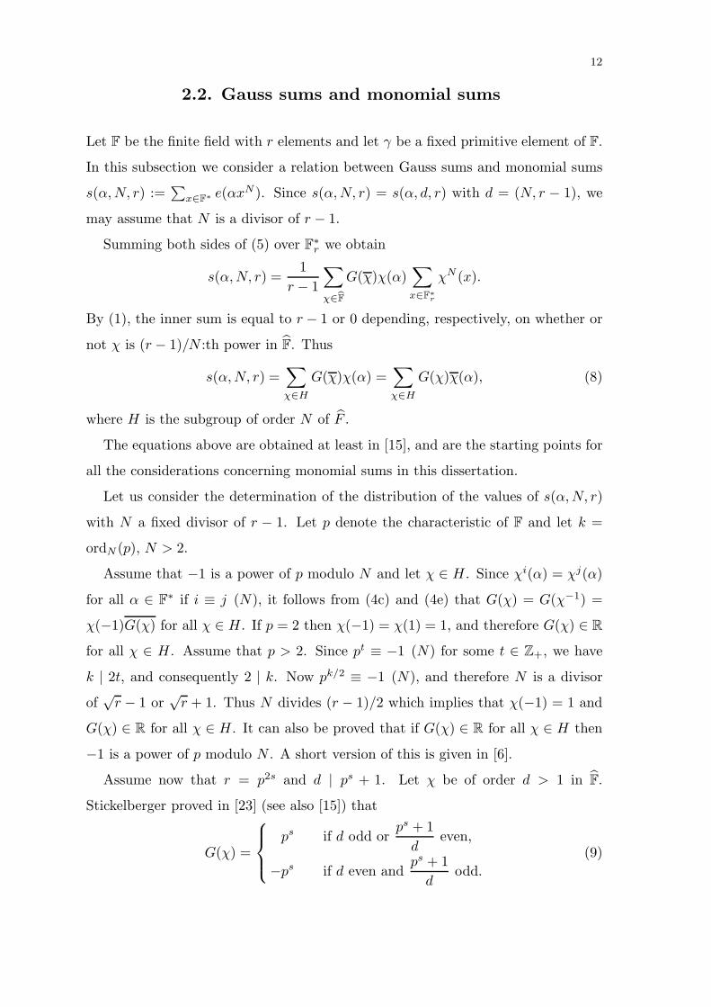
2.2. Gauss sums and monomial sums

Let F be the finite field with r elements and let γ be a fixed primitive element of F.

In this subsection we consider a relation between Gauss sums and monomial sums

s(α,N, r) :=∑

x∈F∗ e(αxN ). Since s(α,N, r) = s(α, d, r) with d = (N, r − 1), we

may assume that N is a divisor of r − 1.

Summing both sides of (5) over F∗r we obtain

s(α,N, r) =1

r − 1

∑χ∈F

G(χ)χ(α)∑x∈F∗

r

χN (x).

By (1), the inner sum is equal to r − 1 or 0 depending, respectively, on whether or

not χ is (r − 1)/N :th power in F. Thus

s(α,N, r) =∑χ∈H

G(χ)χ(α) =∑χ∈H

G(χ)χ(α), (8)

where H is the subgroup of order N of F .

The equations above are obtained at least in [15], and are the starting points for

all the considerations concerning monomial sums in this dissertation.

Let us consider the determination of the distribution of the values of s(α,N, r)

with N a fixed divisor of r − 1. Let p denote the characteristic of F and let k =

ordN (p), N > 2.

Assume that −1 is a power of p modulo N and let χ ∈ H. Since χi(α) = χj(α)

for all α ∈ F∗ if i ≡ j (N), it follows from (4c) and (4e) that G(χ) = G(χ−1) =

χ(−1)G(χ) for all χ ∈ H. If p = 2 then χ(−1) = χ(1) = 1, and therefore G(χ) ∈ R

for all χ ∈ H. Assume that p > 2. Since pt ≡ −1 (N) for some t ∈ Z+, we have

k | 2t, and consequently 2 | k. Now pk/2 ≡ −1 (N), and therefore N is a divisor

of√r − 1 or

√r + 1. Thus N divides (r − 1)/2 which implies that χ(−1) = 1 and

G(χ) ∈ R for all χ ∈ H. It can also be proved that if G(χ) ∈ R for all χ ∈ H then

−1 is a power of p modulo N . A short version of this is given in [6].

Assume now that r = p2s and d | ps + 1. Let χ be of order d > 1 in F.

Stickelberger proved in [23] (see also [15]) that

G(χ) =

⎧⎪⎨⎪⎩ps if d odd or

ps + 1d

even,

−ps if d even andps + 1d

odd.(9)

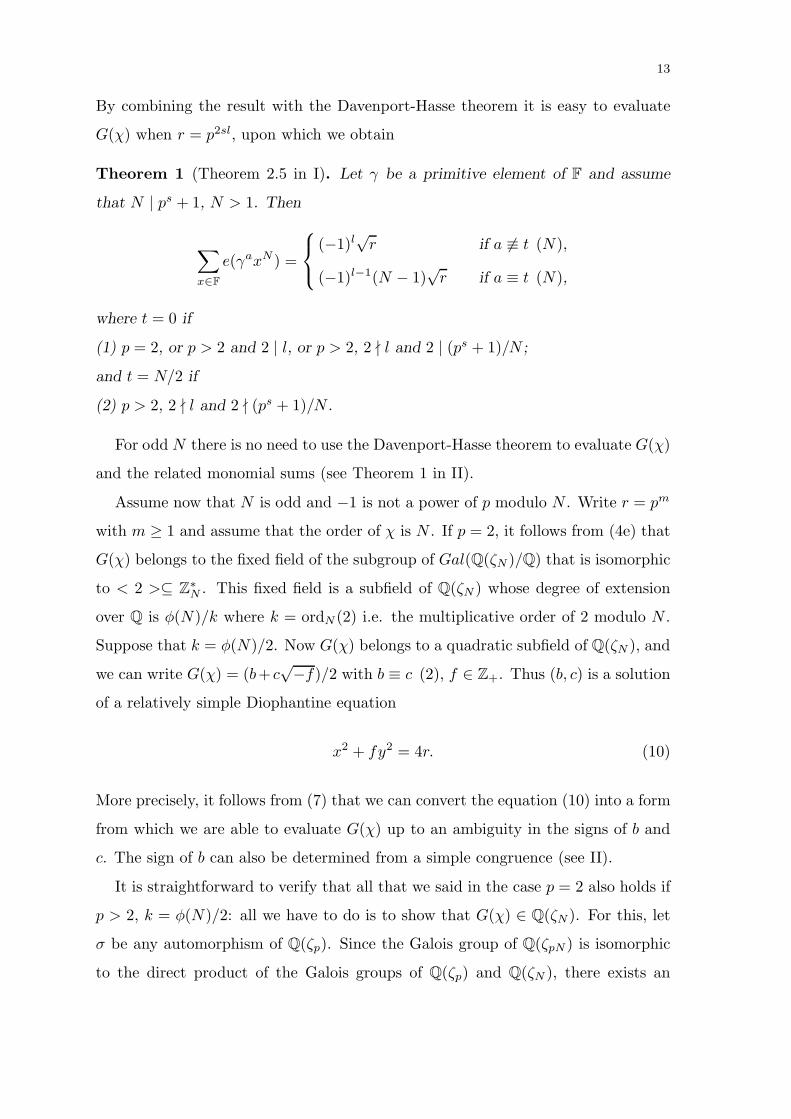
13

By combining the result with the Davenport-Hasse theorem it is easy to evaluate

G(χ) when r = p2sl, upon which we obtain

Theorem 1 (Theorem 2.5 in I). Let γ be a primitive element of F and assume

that N | ps + 1, N > 1. Then

∑x∈F

e(γaxN ) =

⎧⎨⎩ (−1)l√r if a �≡ t (N),

(−1)l−1(N − 1)√r if a ≡ t (N),

where t = 0 if

(1) p = 2, or p > 2 and 2 | l, or p > 2, 2 � l and 2 | (ps + 1)/N ;

and t = N/2 if

(2) p > 2, 2 � l and 2 � (ps + 1)/N .

For odd N there is no need to use the Davenport-Hasse theorem to evaluate G(χ)

and the related monomial sums (see Theorem 1 in II).

Assume now that N is odd and −1 is not a power of p modulo N . Write r = pm

with m ≥ 1 and assume that the order of χ is N . If p = 2, it follows from (4e) that

G(χ) belongs to the fixed field of the subgroup of Gal(Q(ζN )/Q) that is isomorphic

to < 2 >⊆ Z∗N . This fixed field is a subfield of Q(ζN ) whose degree of extension

over Q is φ(N)/k where k = ordN (2) i.e. the multiplicative order of 2 modulo N .

Suppose that k = φ(N)/2. Now G(χ) belongs to a quadratic subfield of Q(ζN ), and

we can write G(χ) = (b+ c√−f)/2 with b ≡ c (2), f ∈ Z+. Thus (b, c) is a solution

of a relatively simple Diophantine equation

x2 + fy2 = 4r. (10)

More precisely, it follows from (7) that we can convert the equation (10) into a form

from which we are able to evaluate G(χ) up to an ambiguity in the signs of b and

c. The sign of b can also be determined from a simple congruence (see II).

It is straightforward to verify that all that we said in the case p = 2 also holds if

p > 2, k = φ(N)/2: all we have to do is to show that G(χ) ∈ Q(ζN ). For this, let

σ be any automorphism of Q(ζp). Since the Galois group of Q(ζpN ) is isomorphic

to the direct product of the Galois groups of Q(ζp) and Q(ζN ), there exists an

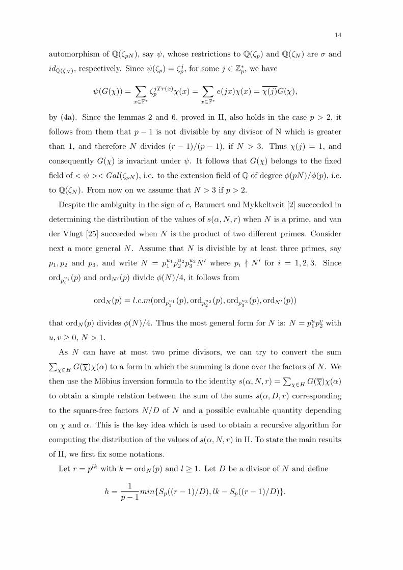
14

automorphism of Q(ζpN ), say ψ, whose restrictions to Q(ζp) and Q(ζN ) are σ and

idQ(ζN ), respectively. Since ψ(ζp) = ζjp, for some j ∈ Z∗

p, we have

ψ(G(χ)) =∑x∈F∗

ζjTr(x)p χ(x) =

∑x∈F∗

e(jx)χ(x) = χ(j)G(χ),

by (4a). Since the lemmas 2 and 6, proved in II, also holds in the case p > 2, it

follows from them that p − 1 is not divisible by any divisor of N which is greater

than 1, and therefore N divides (r − 1)/(p − 1), if N > 3. Thus χ(j) = 1, and

consequently G(χ) is invariant under ψ. It follows that G(χ) belongs to the fixed

field of < ψ >< Gal(ζpN ), i.e. to the extension field of Q of degree φ(pN)/φ(p), i.e.

to Q(ζN ). From now on we assume that N > 3 if p > 2.

Despite the ambiguity in the sign of c, Baumert and Mykkeltveit [2] succeeded in

determining the distribution of the values of s(α,N, r) when N is a prime, and van

der Vlugt [25] succeeded when N is the product of two different primes. Consider

next a more general N . Assume that N is divisible by at least three primes, say

p1, p2 and p3, and write N = pu11 pu2

2 pu33 N ′ where pi � N ′ for i = 1, 2, 3. Since

ordpuii

(p) and ordN ′(p) divide φ(N)/4, it follows from

ordN (p) = l.c.m(ordpu11

(p), ordpu22

(p), ordpu33

(p), ordN ′(p))

that ordN (p) divides φ(N)/4. Thus the most general form for N is: N = pu1p

v2 with

u, v ≥ 0, N > 1.

As N can have at most two prime divisors, we can try to convert the sum∑χ∈H G(χ)χ(α) to a form in which the summing is done over the factors of N . We

then use the Mobius inversion formula to the identity s(α,N, r) =∑

χ∈H G(χ)χ(α)

to obtain a simple relation between the sum of the sums s(α,D, r) corresponding

to the square-free factors N/D of N and a possible evaluable quantity depending

on χ and α. This is the key idea which is used to obtain a recursive algorithm for

computing the distribution of the values of s(α,N, r) in II. To state the main results

of II, we first fix some notations.

Let r = plk with k = ordN (p) and l ≥ 1. Let D be a divisor of N and define

h =1

p− 1min{Sp((r − 1)/D), lk − Sp((r − 1)/D)}.

15

We choose ζ = exp(2πi/N) and normalize the character χ by defining χ(γ) = ζ.

Let

S(a,D) :=∑x∈F∗

e(γaxD),

and let CDa denote the p-cyclotomic coset modulo D defined by a.

It is shown in II that if k = φ(N)/2 and −1 �∈< 2 >⊂ Z∗N , we have three cases

to deal with:

A. N = pu1 , p1 ≡ 3 (4);

B. N = pu1p

v2 , p1 ≡ 1 (4), ordpu

1(p) = φ(pu

1 ) and p2 ≡ 3 (4), ordpv2(p) = φ(pv

2);

C. N = pu1p

v2, p1 ≡ 1, 3 (4), ordpu

1(p) = φ(pu

1 ) and p2 ≡ 3 (4), ordpv2(p) = φ(pv

2)/2.

This result also holds if p > 2, by the proof of lemma 6 in II.

Theorem 2 (Theorem 2 in II). Assume that the case A is valid and let D > 1.

Then

G(χN/D) =b+ c

√−p1

2ph, b, c �≡ 0 (p).

Also, the distribution of the values of S(a,D) can be computed recursively by the

following relations:

(1) S(a,D) =

⎧⎪⎪⎪⎪⎪⎨⎪⎪⎪⎪⎪⎩

φ(D)2

bph + S(0, D/p1) if a = 0,

−D(b− εcp1)ph

2p1+ S(0, D/p1) if a ∈ CD

εD/p1,

S(a,D/p1) otherwise,

where ε ∈ {−1, 1},(2) b2 + p1c

2 = 4pm−2h,

(3) φ(D)bph ≡ −2S(0, D/p1) (D),

(4) S(0, 1) = −1.

We can replace the congruence (3) with (3’), which is easier to use in practical

calculations and implies that G(χN/D) is not a real number (see III):

(3) bph ≡ −2 (p1).

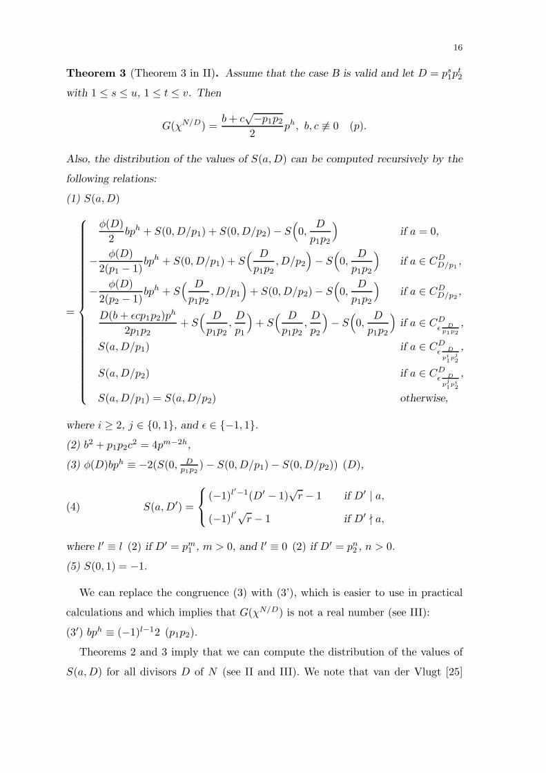
16

Theorem 3 (Theorem 3 in II). Assume that the case B is valid and let D = ps1p

t2

with 1 ≤ s ≤ u, 1 ≤ t ≤ v. Then

G(χN/D) =b+ c

√−p1p2

2ph, b, c �≡ 0 (p).

Also, the distribution of the values of S(a,D) can be computed recursively by the

following relations:

(1) S(a,D)

=

⎧⎪⎪⎪⎪⎪⎪⎪⎪⎪⎪⎪⎪⎪⎪⎪⎪⎪⎪⎪⎪⎪⎪⎨⎪⎪⎪⎪⎪⎪⎪⎪⎪⎪⎪⎪⎪⎪⎪⎪⎪⎪⎪⎪⎪⎪⎩

φ(D)2

bph + S(0, D/p1) + S(0, D/p2) − S(0,

D

p1p2

)if a = 0,

− φ(D)2(p1 − 1)

bph + S(0, D/p1) + S( D

p1p2, D/p2

)− S

(0,

D

p1p2

)if a ∈ CD

D/p1,

− φ(D)2(p2 − 1)

bph + S( D

p1p2, D/p1

)+ S(0, D/p2) − S

(0,

D

p1p2

)if a ∈ CD

D/p2,

D(b+ εcp1p2)ph

2p1p2+ S

( D

p1p2,D

p1

)+ S

( D

p1p2,D

p2

)− S

(0,

D

p1p2

)if a ∈ CD

ε Dp1p2

,

S(a,D/p1) if a ∈ CDε D

pi1p

j2

,

S(a,D/p2) if a ∈ CDε D

pj1pi

2

,

S(a,D/p1) = S(a,D/p2) otherwise,

where i ≥ 2, j ∈ {0, 1}, and ε ∈ {−1, 1}.(2) b2 + p1p2c

2 = 4pm−2h,

(3) φ(D)bph ≡ −2(S(0, Dp1p2

) − S(0, D/p1) − S(0, D/p2)) (D),

(4) S(a,D′) =

⎧⎨⎩ (−1)l′−1(D′ − 1)√r − 1 if D′ | a,

(−1)l′√r − 1 if D′ � a,

where l′ ≡ l (2) if D′ = pm1 , m > 0, and l′ ≡ 0 (2) if D′ = pn

2 , n > 0.

(5) S(0, 1) = −1.

We can replace the congruence (3) with (3’), which is easier to use in practical

calculations and which implies that G(χN/D) is not a real number (see III):

(3′) bph ≡ (−1)l−12 (p1p2).

Theorems 2 and 3 imply that we can compute the distribution of the values of

S(a,D) for all divisors D of N (see II and III). We note that van der Vlugt [25]

17

was able to determine the distribution of the values of S(a,N) in the case C with

N = pq, but we are not able to generalize on this result.

The algorithms in Theorems 2 and 3 are easy to implement, e.g. using MATHE-

MATICA (see Appendix). The critical step from the computational point of view

is the solving of the Diophantine equations. Fortunately, a fast algorithm for that

was developed in [9], and this together with our algorithms allows us to compute

the exponential sums involved in the O(u log r) and O(uv log r) steps, depending on

whether the case is A or B, respectively. We used these algorithms in III to obtain

the weight distributions of certain irreducible cyclic codes.

We finish the discussion concerning monomial sums by considering the absolute

values of s(α,N, r). First we note that taking the absolute values of both sides of

(8) and using (2) and (3), we obtain the Weil bound:

|s(α,N, r)| ≤ (N − 1)√r + 1.

This simple observation is made at least in [15] and [22]. Theorem 1 shows that the

Weil bound is obtained for certain divisors N <√r of r − 1. On the other hand

Theorems 3 and 4 imply that the Weil bound is never obtained if one of the cases

A or B above is valid, since the Gauss sums involved are not real.

We next consider the sums s(α,N, r), for which the Weil bound is often too weak,

i.e. when N is large with respect to√r. We shall first fix some notations.

Let F denote the finite field with q elements and let E denote the extension field

of F with r = qm elements. Let e and ψ denote the canonical additive characters

of E and F , respectively. Let n ∈ Z+, β ∈ F ∗ and define an n-dimensional (or

multiple) Kloosterman sum over F

Kn(β) =∑

x∈F ∗ψ(x1 + · · ·+ xn + βx−1

1 . . . x−1n ).

We obtain from the Davenport-Hasse theorem the following relation between

monomial sums and (m− 1)-dimensional Kloosterman sums.

18

Theorem 4 (Theorem 2.2 in I). For all α ∈ E∗

s(α, q− 1, r) = (−1)m−1∑χ∈ F

g(χ)mχ(NE/F (α)) = (−1)m−1(q− 1)Km−1(NE/F (α)),

where g(χ) is a Gauss sum over F and NE/F is the norm mapping from E to F .

Let N be a divisor of q − 1. Since we have a partition of the group of the N -th

powers of E∗ into the cosets of the subgroup of (q − 1):th powers we can convert

the sum s(α,N, r) into a sum of (m − 1)-dimensional Kloosterman sums over F .

The Deligne bound

|Kn(α)| ≤ (n+ 1)qn/2

now implies

Corollary 1 (Corollary 2.4 in I). Let α ∈ E∗ and N | q − 1. Then

∣∣s(α,N, r)∣∣ ≤ m(q1/2 − q−1/2)√r.

Deligne’s difficult proof is contained in [5].

Theorem 4 also implies

Corollary 2 (Corollary 2.3 in I). Let β ∈ F∗. Then

|Kn(β)| ≤ qn+12 − q

n+12 − 1q − 1

.

The bound in corollary 2 is practically the same as the bound

|Kn(β)|2 ≤ qn+1 − qn+1 − 1q − 1

obtained in [12], and is a generalizion and a slight improvement of the classical

bound |Kn(β)| ≤ qn+1

2 proved by Mordell for the prime q in [21].

Assume now that r = pm with m > 0 even and consider the sums s(α,N, r),

α �= 0. We may write N = dt where d | q + 1 and t | q − 1 with q = pm/2. We have

19

already dealt with the cases where d = 1 or t = 1, and so we assume that d, t > 1.

Because of the partition < γdt >=⋃ q+1

d −1i=0 γdti < γ(q+1)t >, we have

s(α,N, r) = dt

q+1d −1∑i=0

q−1t −1∑j=0

e(αγdtiγ(q+1)t)

= d

q+1d −1∑i=0

∑x∈K∗

ψ(TrF/K(αγdti)xt),

where K is the subfield of F with q elements and ψ is the canonical additive character

of K.

If α ∈ K then s(α,N, r) = r − 1. Assume α �∈ K.

If p = 2 and α �∈ K, then TrE/K(αγdti) = 0 if and only if dti ≡ −indγ(α) (q+1).

Also, the congruence is solvable if and only if d | indγ(α), and so there exists at

most one i ∈ {0, . . . , (q + 1)/d− 1} for which the congruence is solvable. Now, by

the Weil bound, we have

Theorem 5.

|s(α, dt, r)|

≤⎧⎨⎩ ((t− 1)r1/4 + d+ 1)

√r − (d− 1)(t− 1)r1/4 − 2d+ 1 if indγ(α) ≡ 0 (d),

(t− 1)r1/4√r + (t− 1)r1/4 + 1 if indγ(α) �≡ 0 (d).

If p > 2, then TrE/K(αγdti) = 0 if and only if dti ≡ (q+1)/2−indγ(α) (q+1). It

is easy to see that (dt, q+1) is equal to 2d if 2 | t and d < q+1 (Case 1). Otherwise

it equals d (Case 2). Now we have

Theorem 5’. If indγ(α) ≡ (q + 1)/2 (nd) then

|s(α, dt, r)| ≤ ((t− 1)r1/4 + nd+ 1)√r − (nd− 1)(t− 1)r1/4 − 2nd+ 1;

otherwise

|s(α, dt, r)| ≤ (t− 1)r1/4√r + (t− 1)r1/4 + 1,

where n = 1 or 2 depending on whether Case 1 or Case 2 is valid, respectively.

We observe that our bounds are better than the Weil bound if d > r1/4, for

example.

20

2.3. Gauss sums and binomial sums

Let f = αXN + βX ∈ F[X ], α, β ∈ F, α �= 0. Let us denote

s(α, β,N, r) :=∑x∈F∗

e(αxN + βx).

Two methods come to mind for studying the sums s(α, β,N, r) with β �= 0 using

Gauss sums. First, expanding e(αxN ) using (5), we arrive at the relation

s(α, β,N, r) =1

r − 1

∑χ∈F

G(χ)G(χN )χ(αβ−N ). (11)

On the other hand, expanding e(βx) using (5) leads us to the relation

s(α, β,N, r) =1

r − 1

∑χ∈F

G(χ)χ(β)∑x∈F∗

χ(x)e(αxN ). (12)

We see that we can convert the sum s(α, β,N, r) into a simpler form if we can

evaluate G(χN ) or the product of the Gauss sums G(χ)G(χN ) or hybrid sums∑x∈F∗ χ(x)e(αxN ). These are in general hard tasks, but as we shall see, they can

be achieved in certain special cases.

If (N, r − 1) = 1, the substitution x �→ xt makes the inner sum in (12) to be

χ(α−t)G(χt) by (4a), if t is the inverse of N modulo r−1. Thus, no matter whether

the starting point is (11) or (12), we have to analyze the sums of the products of

two Gauss sums.

Assume now that N | r− 1, N > 1. Let F denote the finite field with q elements

and let E denote the extension field of F with r = qm elements. Let e and ψ denote

the canonical additive characters of E and F , respectively.

Let us first consider (11). Let H be the subgroup of order N of E. Let us fix a

generator of E, say λ. Denote J := {0, . . . , (r − 1)/N − 1}. Now {λj | j ∈ J} is a

complete set of representatives of the cosets of H, and we have

s(α, β,N, r) =1

r − 1

( ∑j∈J\{0}

G(λNj)∑χ∈H

G(λjχ)(λjχ)(αβ−N )−∑χ∈H

G(χ)χ(αβ−N )).

We see that it may be possible to convert the above sum into a simpler form if

we can evaluate G(λNj). We assume that N = (r− 1)/(q+ 1) and m is even, since

we can then use (9). Let M denote the field satisfying F ⊆M ⊆ E, [M : F ] = 2.

21

Let us fix a generator of M , say λM , by setting λM (NE/M (γ)) = λt(γ), where

t = (r−1)/(q2−1) and γ is a primitive element of E. It follows from the Davenport-

Hasse theorem that G(λNj) = (−1)m/2−1g(λ(q−1)jM )m/2, where g(λ(q−1)j

M ) is a Gauss

sum over M . Denote ε = (−1)m/2−1. Since ord(λ(q−1)jM ) = (q + 1)/(q + 1, j),

it follows from (9) that g(λ(q−1)jM ) = −q if and only if j and q are odd. Thus

G(λNj) = ε√r if 2 | q or 2 | m/2, and otherwise G(λNj) = ε(−1)j

√r. In the latter

case we also have (−1)j(λjχ)(αβ−N ) = (λjχ)(−αβ−N ), since χ(−1) = 1 for all

χ ∈ H. Now, by (8), we obtain

s(α, β,N, r) =1

r − 1

(ε√r

∑j∈J\{0}

∑χ∈H

G(λjχ)(λjχ)(±αβ−N ) −∑χ∈H

G(χ)χ(αβ−N ))

=1

r − 1

(ε√r

∑χ∈ E

G(χ)χ(±αβ−N ) − (ε√r + 1)

∑x∈E∗

e(αβ−NxN )).

It follows from (5) that

s(α, β,N, r) = ε√re(±αβ−N ) − 1

ε√r − 1

∑x∈E∗

e(αβ−NxN ), (13)

where the + sign holds if and only if 2 | q or m ≡ 0 (4). To handle the monomial

sum in (13) we need a simple

Lemma (Proposition 2.6 in I).

∑x∈E∗

e(αxr−1q+1 ) =

⎧⎨⎩r − 1 if TrE/M (α) = 0,

−r − 1q + 1

K1

(NM/F (TrE/M (α))

)if TrE/M (α) �= 0.

Now, by (13) and this lemma, we have

Theorem 6 (Theorem 2.7 in I). Let α, β ∈ E, β �= 0 and assume that m is even.

Then

s(α, β,r − 1q + 1

, r) =

⎧⎨⎩− 1 if TrE/M (α) = 0,

(−1)m/2−1e(±δ)√r +(−1)m/2−1

√r + 1

q + 1K1(ν) if TrE/M (α) �= 0,

where δ = αβ− r−1q+1 , ν = NM/F (TrE/M (δ)) and the − sign holds if and only if m ≡ 2

(4).

Corollary 3. Let α, β ∈ E, β �= 0 and assume that m is even. Then

|s(α, β, r − 1q + 1

, r)| ≤( 2r

12m

r1m + 1

+ 1)√

r +2r

12m

r1m + 1

22

We shall next consider (12):

s(α, β,N, r) =1

r − 1

∑χ∈ E

G(χ)χ(β)∑

x∈E∗χ(x)e(αxN ).

Let us fix a primitive element of E, say γ. Let T be a subgroup of order N of E∗

and denote J := {0, . . . , (r−1)/N−1}. The set S := {γj | j ∈ J} is now a complete

set of representatives of cosets of T in E∗. Obviously∑x∈E∗

χ(x)eE(αxN ) =∑j∈J

χ(γj)e(αγNj)∑x∈T

χ(x),

and∑

x∈T χ(x) = N or 0 depending on whether ord(χ) divides (r − 1)/N or not.

Let λ denote a generator of E. Now

s(α, β,N, r) =N

r − 1

∑i∈J

G(λNi

)λNi(β)∑j∈J

λNi(γj)e(αγNj).

Let us fix a generator of F , say λF , by setting λF (NE/F (γ)) = λt(γ), where

t = (r − 1)/(q − 1). Assume that N = t. The inner sum is now nothing more than

a Gauss sum g(λiF , ψδ) over F where ψ is the canonical additive character of F and

δ = TrE/F (α). By the Davenport-Hasse theorem, we now have

s(α, β,N, r) =(−1)m−1

q − 1

∑i∈J

g(λi

F )mg(λiF , ψδ)λi

F (NE/F (β))

=(−1)m−1

q − 1

∑χ∈ F

g(χ)mg(χ, ψδ)χ(NE/F (β)).

Assume that δ = 0. Now g(χ, ψδ) = q−1 or 0, depending on whether χ is trivial

or not. Thus

s(α, β,N, r) =(−1)m−1

q − 1(−1)m(q − 1) = −1.

Assume that δ �= 0. Now g(χ, ψδ) = χ(δ)g(χ). We also have g(χ)g(χ) = χ(−1)q,

if χ is not the trivial character χ0. Consequently,

s(α, β,N, r) =(−1)m−1q

q − 1

∑χ∈ F\{χ0}

g(χ)m−1χ(−NE/F (β)TrE/F (α)−1) +1

q − 1

=(−1)m−1q

q − 1

∑χ∈ F

g(χ)m−1χ(−NE/F (β)TrE/F (α)−1) − 1.

If m = 2, we obtain by (5)

23

Theorem 7 (Theorem 2.8 in I). If α, β ∈ E, β �= 0. Then

∑x∈E∗

e(αxq+1 + βx) =

{ − 1 if α+ αq = 0,

− qψ(−βq+1(α+ αq)−1) − 1 if α+ αq �= 0,

Assume that m > 2. Let E′ be an extension field of degree m − 1 over F .

Because of the surjectivity of the norm mapping, we can choose ν ∈ E′ such that

NE′/F (ν) = −NE/F (β)TrE/F (α)−1. By Theorem 4, we now obtain

∑x∈E′∗

eE′(νxq−1) = (−1)m−2∑χ∈ F

g(χ)m−1χ(−NE/F (β)TrE/F (α)−1).

We have thus proved

Theorem 8 (Theorem 2.9 in I). Let α, β ∈ E, β �= 0. If m > 2 then

s(α, β,r − 1q − 1

, r) =

{ − 1 if TrE/F (α) = 0,

(−1)m−1qKm−2(−NE/F (β)TrE/F (α)−1) − 1 if TrE/F (α) �= 0.

Corollary 4. Let α, β ∈ E, β �= 0. Then

|s(α, β, r − 1q − 1

, r)| ≤ (m− 1)√r + 1.

The case β = 0 is easy to deal with:

∑x∈E∗

e(αxr−1q−1 ) =

r − 1q − 1

∑y∈F ∗

ψ(TrE/F (α)y) =

⎧⎨⎩r − 1 if TrE/F (α) = 0,

−r − 1q − 1

if TrE/F (α) �= 0.(14)

Thus our study of s(α, β, (r− 1)/(q − 1), r) is completed.

Now that we have found these results, we may try to find simpler proofs for

them. This is done in I by starting from the equation

s(α, β,N, r) =t−1∑i=0

e(αγNi)∑

x∈γi<γT >

e(βx), (15)

where T = (r − 1)/N .

24

We conclude the discussion of binomial sums by considering the sums

s(α, β,N, T, r) :=∑x∈F∗

e(αxN + βxT ),

where N is a divisor of r − 1 greater than 1 and NT = r − 1. We could proceed as

in the proof of Theorem 8, but instead of that we start from (15).

Since we have a partition F∗ =⋃N−1

i=0 γi < γN >, we obtain

s(α, β,N, T, r) =N−1∑i=0

e(βγTi)∑

x∈<γN >

e(αγNixN ).

Assume now that (N, T ) = 1. It follows that the mapping x �→ xN is a permutation

of < γN >, and therefore

∑x∈<γN >

e(αγNixN ) =∑

x∈<γN >

e(αγNix) =∑

x∈<γN >

e(αx).

Thus

s(α, β,N, T, r) = (∑

x∈<γN >

e(αx))(∑

x∈<γT >

e(βx)),

and we have

Theorem 9. Let NT = r − 1 with N > 1. If (N, T ) = 1, then

s(α, β,N, T, r) =s(α,N, r)s(β, T, r)

r − 1.

Corollary 5. Let r = 22n. Then

|s(α, β, 2n − 1, 2n + 1, r)| ≤⎧⎨⎩ 2r1/4 if β �= β2n

,

2r1/4(√r − 1) if β = β2n

,

Proof. Since (2n − 1, 2n + 1) = 1, the bound follows from Theorems 1 and 9 and

corollary 1. �

25

2.4. Coding theoretic applications

In this subsection we give interpretations in terms of coding theory for the results

obtained so far. We first state some preliminaries concerning binary cyclic codes.

For more complete descriptions, see [17] and [10].

Let Fn2 denote the n-dimensional vector space over F2, and let C be a k-dimensional

subspace of Fn2 . We call C a linear [n, k]-code over F2, and an element of C a code-

word (of C). The weight w(c) of a codeword c ∈ C is the sum of the coordinates of

c. Let Ni denote the number of codewords of C of weight i. The weight distribution

of C is the set W (C) := {(i, Ni) | i = 0, 1, . . . n,Ni �= 0} and the minimum distance

of C is the weight of the non-zero codeword with smallest weight.

Assume now that C is invariant under the cyclic shift of the coordinates of every

codeword of C. Such a code is called cyclic. There is a one to one correspondence

between the cyclic [n, k]-codes C and the ideals I of the residue class ring Rn :=

F2[X ]/ < Xn+1 > (see [17]). Furthermore, we may think a codeword (a0, . . . , an−1)

of C as an element a0 + a1X + . . . , an−1Xn−1+ < Xn + 1 > of I, and conversely.

Let I be an ideal of Rn and let C be the corresponding cyclic code. We know

that I is generated by an element g(X)+ < Xn + 1 >, where g(X) is a divisor of

Xn + 1 in F2[X ] (see [17]). We call g(X) the generator polynomial of C and the

zeros of g(X) in the splitting field of Xn + 1 the zeros of C. The cyclic code with

the generator polynomial Xdeg h(X)h(X−1) with h(X) = (Xn + 1)/g(X) is called

the dual of C.

Let r = 2m and nN = r− 1. Let F denote the field with r elements and let γ be

a primitive element of F. Any cyclic code of length n has a very simple description

by means of the trace function. In fact, let P be an additive subgroup of F2[X ] and

define a linear code C of length n by setting

C = C(P ) = {c(f) | f ∈ P},

where

c(f) = (Tr(f(1)), T r(f(γ)), . . . , T r(f(γn−1))).

It is shown in [10] that the dual of a cyclic code B of length n with zeros γNs1 , . . . , γNsu

26

is the code C(P ) with P = {∑ui=1 aiX

Nsi | ai ∈ F}. Since the dual of the dual of Bis B, every cyclic code has the above description.

Let us consider the weight of a word c(f) of the cyclic code C(P ) with P =

{∑ui=1 aiX

Nsi | ai ∈ F}. Clearly

w(c(f)) =12

n−1∑j=0

(1 − e(u∑

i=1

aiγNsij))

=12(n−

n−1∑j=0

e(u∑

i=1

aiγNsij))

=1

2N(r −

∑x∈F

e(u∑

i=1

aixNsi)). (16)

Thus the determination of the weight distribution of C is an equivalent task to the

determination of the distribution of the values of∑

x∈F e(f(x)) with f(X) ∈ P .

Let us now consider more closely the cyclic code C(P ) with all si’s in the same

2-cyclotomic coset modulo n defined by s := s1. In other words C := C(P ) is

the dual of the code B with an irreducible generator polynomial g(X) (see [17]).

Consequently, the generator polynomial of C is h(X) := (Xn+1)/f(X) with f(X) =

Xdeg g(X)g(X−1). Since f(X) is irreducible, it follows that the ideal generated by

h(X)+ < Xn+1 > is a minimal ideal of Rn. In other words, C contains no subspace

�= 0 which is closed under the cyclic shift operator. Code C is called an irreducible

cyclic code, since the ideal corresponding to C cannot be written non-trivially as

the sum of its subideals.

The dimension dim C(P ) of C over F2 is easy to determine. Since the number

of elements on the 2-cyclotomic coset modulo n defined by s is equal to ordn′(2)

with n′ = n/(n, s), deg g(X) = ordn′(2). Since dim C = n − deg h(X) (see [17]),

dim C(P ) = ordn′(2).

As Tr(αx2) = Tr(√αx) for all α ∈ Fr we arrive at the following result proved

by van Lint in [16]: The set

C = {c(α) := (Tr(α), T r(αγN), . . . , T r(αγ(n−1)N)) | α ∈ F}

is an irreducible cyclic code of dimension ordn(2) over F2.

27

Let F be a homomorphism from (F,+) to C defined by α �→ c(α). Each codeword

occurs |Ker(F )| = 2m−ordn′(2) times in C. We call C a degenerate code if m >

ordn′(2). Otherwise we call C a non-degenerate code. Denote d = (n, s). A sufficient

condition for the bijectivity of F is Nd <√r+1, since for α �= 0, |∑x∈F e(αx

Ns)| ≤(Nd − 1)

√r. Furthermore, this condition holds if m/ ordNd(2) ≥ 2, since then

Nd ≤ √r − 1.

Example 1. Let N = 1. The code C(P ) with P = {αx | α ∈ F} is now the dual

of the Hamming code of length 2m − 1 i.e. the dual of a [2m − 1, n − ordn(2)] =

[2m − 1, 2m −m − 1] code. The [2m − 1, m] code C(P ) is called the Simplex code.

The weight distribution of C(P ) is {(0, 1), (2m−1, 2m − 1)}, by (1) and (16).

Example 2. Let N > 1 and −1 ∈< 2 >⊂ Z∗N . Now the code C(P ) with P =

{αxN | α ∈ F} is an irreducible cyclic [(2m − 1)/N,m] code. The dimension is m,

since N <√r+1 (see the discussion after (8)). The weight distribution of the code

is {(0, 1), (w1, (r − 1)/N), (w2, (N − 1)(r − 1)/N)}, where

w1 =1

2N(r + (−1)l(N − 1)2m/2), w2 =

12N

(r + (−1)l−12m/2),

with l = m/ ordN (2), by Theorem 1 and (16).

Example 3. Let ordN (2) = φ(N)/2 and assume that −1 �∈< 2 >⊂ Z∗N . Suppose

that case A or B is valid (see Theorems 2 and 3). The code C(P ) with P = {αXN |α ∈ F} is an irreducible cyclic [(2m − 1)/N, ordn(2)]-code. The weight distribution

of the code can be computed by Theorems 2 and 3. See also III, where algorithms

for the computation of the weight distributions and also some weight distributions

are presented, and the Appendix for the implementation of these algorithms using

MATHEMATICA .

Denote q = 2t, t > 1 and r = qm, m > 1.

Example 4. Let N = q − 1. The code C(P ) with P = {αXN | α ∈ F} is an

irreducible cyclic [(qm − 1)/(q − 1), mt] code, since mt/ordN (2) ≥ 2. The weight of

any word c := c(α) ∈ C(P ), α �= 0, satisfies the inequality

|2w(c) − n| ≤ min{mq(m−1)/2,√qq(m−1)/2 − qm/2 − 1

q − 1},

28

by corollary 1 and the Weil bound.

The first two examples are well known (see e.g. [17] ). Example 4 is from I. If

m = 2, the dual in example 4 is the dual of the Zetterberg code (see [17]), in which

case it has been studied at least in [13] and [20].

Let us again consider C := C(P ) with P = {∑ui=1 aiX

Nsi | ai ∈ F}. Let us

assume that all si’s lie in different 2-cyclotomic cosets modulo n. It follows from

the linearity of the trace map that the ideal corresponding to C is the sum of the

ideals corresponding to Ci := C(Pi) with Pi = {αXNsi | α ∈ F}. Since the ideals

corresponding to Ci are minimal, it follows that the sum is direct. We say that the

cyclic code C is the direct sum of irreducible cyclic codes Ci. Clearly the dimension of

C is∑u

i=1 ordn′i(2) with n′

i = n/(n, si). Furthermore, dim C = um if NM ≤ √r+1

with M = max{(n, si)}, and this condition is satisfied if m/ ordNM (2) ≥ 2.

Example 5. Let N = 1 and m = 2. The code C(P ) with P = {αXq+1 + βX |α, β ∈ F} is a cyclic [q2 − 1, 3t] code since ordq2−1(2) = 2t and ordq−1(2) = t. The

code is the direct sum of the Simplex code of length q2−1 and the irreducible cyclic

code obtained by pasting together q + 1 copies of the Simplex code of length q− 1.

The weight distribution of the code is

{(0, 1), (22t−1−2t−1, 2t−1(22t−1)), (22t−1, 22t−1), (22t−1+2t−1, 23t−1−22t +2t−1)}

by the following discussion.

Denote

c(α, β) =(Tr(α+ β), T r(αγ2t+1 + βγ), . . . , T r(αγ(2t+1)(r−2) + βγr−2)

) ∈ C(P ).

If c(α′, β′) ∈ C(P ) it follows from the linearity of the trace map and from Theorems

1 and 7 that c(α, β) = c(α′, β′) if and only if T (α) = T (α′) and β = β′, where

T is the trace map from F to its subfield with 2t elements, say K. Let β be a

fixed element of F∗. If α runs over all elements of F satisfying T (α) �= 0, then

T (β2t+1(α + α2t

)−1) runs over all elements of K∗. There exist 2t−1 − 1 elements

δ ∈ K∗ satisfying TrK/F2(δ) = 0 and 2t−1 elements δ ∈ K∗ satisfying TrK/F2(δ) = 1.

29

We now let β vary over F∗ and it follows from Theorem 7 that there are 2t−1(22t−1)

codewords of weight 22t−1 − 2t−1, (2t−1 − 1)(22t − 1) words of weight 22t−1 + 2t−1,

and 22t −1 words of weight 22t−1 in C(P ). Let β = 0. It now follows from Theorem

1 that there are 2t−1 words more of weight 22t−1 +2t−1 and the zero word in C(P ).

Example 6. Let N = 1 and m > 2. The code C(P ) with P = {αXd + βx | α, β ∈Fr}, d = (qm−1)/(q−1), is a cyclic [qm−1, (m+1)t]-code. It follows from Theorem

8, Corollary 2, Corollary 4 and (14) that there are

(1) qm − 1 words of weight qm/2 and

(2) q − 1 words of weight (qm − 1 + (qm − 1)/(q − 1))/2

in the code C(P ). For the remaining (qm − 1)(q − 1) words c �= (0, . . . , 0) we have

(3) q − 1 ≤ |2w(c) − n| ≤ min{√qqm/2 −√

qqm/2−q

q−1 + 1, (m− 1)qm/2 + 1}.This code is a small subcode of m-th order punctured Reed-Muller code R∗(m, tm)

(see [10] for the trace function description of Reed-Muller codes). We note that the

weights in Cases 2 and 3 are exactly divisible by 2t−1 which is in accordance with

the divisibility result of McEliece [18] (see also [17]) which states that the weights of

an arbitrary Reed-Muller code R(l, u) are divisible by 2�ul �−1, but not necessarily

exactly. This example also shows us that it may be difficult to determine the weight

distribution of R(l, u) if l > 2 and l | u, since we the have to be able to compute

the distribution of the values of multiple Kloosterman sums (see Research Problem

15.1 in [17]). We can go further in the example if we assume that m = 3, i.e. the

code under consideration is a [23t − 1, 4t] subcode of R∗(3, 3t). It is proved in [13]

that the set of values of Kloosterman sum K1(α) over the field of order q is equal

to the set {i | i ∈ [−2√q, 2

√q], i ≡ −1 (4)}. Thus we can replace (3) by

(3’) The set of the weights of the remaining (q3 − 1)(q − 1) non-zero codewords is

equal to the set

{12q(qm−1 − i) | i ∈ [−2

√q, 2

√q], i ≡ −1 (4)}.

30

3. References

1. Baumert LD & McEliece RJ (1972) Weights of irreducible cyclic codes. Inform.and Control 20: 158-175.

2. Baumert LD & Mykkeltveit J (1973) Weight distributions of some irreduciblecyclic codes. JPL Tech. Report 32-1526: 128-131.

3. Berndt BC & Evans RJ (1981) The determination of Gauss sums. Bull. Am.Math. Soc. 5: 107-129.

4. Davenport H & Hasse H (1935) Die Nullstellen der Kongruenz Zetafunktion ingewissen zyklischen Fallen. J. Reine und Angew. Math. 172: 151-182.

5. Deligne P (1977) Applications de la formule des traces aux sommes trigonometriques.SGA 4 1/2 Springer Lecture Notes in Math 569: 168-232. Springer, New York.

6. Evans RJ (1981) Pure Gauss sums over finite fields. Mathematika 28: 239-248.7. Gauss CF (1965) Arithmetische Untersuchungen. Chelsea, New York.8. Hardy K, Muskat JB & Williams KS (1990) A deterministic algorithm for solving

n = fu2 + gv2 in coprime integers u and v. Math. Comp. 55: 327-343.9. Hasse H (1964) Vorlesungen uber Zahlentheorie. Grudl. der Math. Wiss. Vol.

59. Springer-Verlag, Berlin.10. Honkala I & Tietavainen A (to appear) Codes and Number Theory. In: Brualdi

RA, Huffman WC & Pless V (eds) Handbook of Coding Theory. Elsevier SciencePublisher, Amsterdam.

11. Ireland K & Rosen M (1982) A Classical Introduction to Modern Number Theory.Grad. Texts in Math. Vol. 84. Springer-Verlag, New York.

12. Katz NM (1980) Sommes Exponentielles. Soc. Math. France 79. Paris.13. Lachaud G & Wolfman J (1990) The weights of the orthogonals of the extended

quadratic binary Goppa codes. IEEE Trans. Inform. Theory 36: 686-692.14. Langevin P (1997) Calculus de certaines sommes de Gauss. J. Number Theory

32: 59-64.15. Lidl R & Niederreiter H (1984) Finite Fields. Cambridge Univ. Press, Cambridge.16. van Lint J. H. (1982) Introduction to Coding Theory. Springer-Verlag, New York.17. MacWilliams FJ & Sloane NJA (1978) The Theory of Error-Correcting Codes.

North-Holland, Amsterdam.18. McEliece RJ (1972) Weight congruences for p-adic cyclic codes. Discrete Math.

3: 177-192.19. McEliece RJ (1974) Irreducible cyclic codes and Gauss sums. In: Hall M Jr & van

Lint JH (eds) Combinatorics (Part 1): 179-196. Mathematical Centre Tracts 55,Mathematical Centre, Amsterdam.

20. McEliece RJ (1980) Correlation properties of sets of sequences derived from irre-ducible cyclic codes. Inform. and Control 45: 18-25.

21. Mordell LJ (1963) On a special polynomial congruence and exponential sums. In:Calcutta Math. Soc. Golden Jubilee Commemoration Volume, Part 1: 29-32.Calcutta Math. Soc., Calcutta.

22. Schmidt WM (1976) Equations over Finite Fields: An Elementary Approach.Springer, Berlin.

23. Stickelberger L (1890) Uber eine Verallgemeinerung von der Kreistheilung. Math.Ann. 37: 321-367.

24. Stichtenoth H (1993) Algebraic Function Fields and Codes. Springer-Verlag, Uni-versitext, New York.

25. van der Vlugt M (1995) Hasse-Davenport curves, Gauss sums, and weight distri-butions of irreducible cyclic codes. J. Number Theory 55: 145-159.

31

26. Weil A (1948) On some exponential sums. Proc. Natl. Acad. Sci. 34: 204-207.

Appendix: Computer programs

Original articles

See my homepage.