Exponential growth, energetic Hubbertcycles, and the advancement of technology

Tad W. Patzek

Department of Civil and Environmental Engineering425 Davis Hall, MC 1716

University of California, Berkeley, CA 94720Email: patzek@patzek.berkeley.edu

Accepted by the Archives of Mining Sciences of the Polish Academy of Sciences, May 3, 2008

May 17, 2008

Abstract

In the recovery of geologic fossil fuel deposits, the overall production rate first goesup and then it must come down. Tens of thousands of oil and gas fields in the worldproduce hydrocarbons at rates that have long-time tails, making them highly asymmetricfunctions of time. Yet the sums of annual production volumes from these fields follow sym-metric Gaussian distributions in time, also known as “Hubbert cycles.” This paper providesmathematical arguments for the existence of energetic Hubbert cycles and their practicalequivalence to the logistic growth curves. It is shown that the rates of oil production in theworld and in the United States doubled 10 times, each increasing by a factor of ca. 1000,before reaching their respective peaks. The famous peak of US oil production occurred in1970, and global oil production probably peaked in 2005 – 2006, with little fanfare. Therate of natural gas production in the US has also increased by a factor of 1000 and is at itssecond peak as of this writing in April 2008. The multi-Hubbert cycle analysis of oil andgas production in America emphasizes the existence of new populations of reservoirs, rathersmall in the case of oil production, but very large in the case of gas production. It turnsout that improved technology and new science have allowed the oil producers in America toincrease ultimate recovery by 2 years of total energy consumption in the United States. TheAmerican producers of natural gas, mostly small independents, are on a path of achievingan increase of ultimate gas production larger than 10 years of total energy consumption inthe United States. Thus, the discounted cumulative value of good science and engineeringin the American oil and gas industry is worth well over 1 trillion USD in 2008, and it willcontinue to grow exponentially in the near future, given the declining oil and gas produc-tion rates and the high prices of both commodities. Producing the undiscovered technicallyproducible petroleum from the ANWR 1002 Area, as well as the known gas caps in PrudhoeBay and Point Thompson, all in Alaska, will have a small impact on the energy supply ofthe Unites States.

1 Introduction

Just like bacteria, fungi, and higher animals, humans continuously seek new sources of cheap,accessible organic carbon. Starting from the soil and crop carbon, through the wood carbon inforests, and ending with coal, petroleum and natural gas, humans have developed an insatiableappetite for power from the temporarily abundant and fungible sources of carbon energy.

1

1.1 Background

The happy whales in Figure 1 were thanking Colonel Drake and others for introducing kerosene(paraffin oil) as a cheap abundant alternative to blubber oil. The truth was more complicated(Ellis, 1991). Because of prior investment into the steel-hull, steam-powered, canon-equippedships, whale hunting continued until whales neared extinction. Fast forward 150 years. By2008, the gigantic agrofuel plantations have invaded land in the tropics, destroying some of themost important ecosystems on the planet. Even when we collectively discover the impossibilityof replacing geologic carbon accumulations with annual carbon flows (explained below), theindiscriminate hunt of ecosystems will continue because large monetary investments are neverabandoned of free will.

Figure 1: The introduction of drill pipes was key to striking oil near Titusville, Pennsylvania,on August 27, 1859. These jubilant whales, depicted by Vanity Fair on April 20, 1861, werethankful to Seneca Oil for saving them from extinction.

1.2 Resources

The Earth and her crust are made of stellar matter, and the current abundance of each chemicalelement and its compounds (minerals, ores, etc.) results from chemical composition of thatprimordial matter and the geologic evolution of the Earth. The Sun powers the Earth; life hasevolved her atmosphere, stabilized the climate, and made all fossil fuels, coal, crude oil, naturalgas, gas hydrates, oil shale, etc. The deposition and transformation rates of these fossil fuelsare very slow (Patzek and Pimentel, 2006). It is the unimaginable length of deposition time,measured in hundreds of millions of years, that accumulated large quantities of these fuels, seeFigure 2. In a few hundred years, a geological blink of an eye, humans will practically exhaustthe fossil fuels.

All resources that feed our civilization: the highly concentrated or pure (“low-entropy”)compounds (Georgescu-Roegen, 1971) – clean water, clean air, pure minerals, finished metals,high-quality fossil fuels, wood, uncontaminated food –, as well as the self-sustaining ecosystems

2

0 5000580

500

436

396

345

310

281

232

196

141

66

23 2

Late Tertiary

Early Tertiary

Cretaceous

Jurassic

Triassic

Permian

Late Carbonif.

Early Carbonif.

Devonian

Sylurian

Ordovician

Cambrian

MY

r

m3/Yr

Heavy Oil

0 5000

m3/Yr

Oil

0 2000

Gas

1000 m3/Yr

50 1501000 t/Yr

Coal

Figure 2: The average rates of accumulation of fossil fuels in the Earth over geological time.The average rates of heavy oil deposition are from Demaison (1977). The average rates of oiland gas deposition are from Bois et al. (1982). The coal deposition rates are from Bestoug-eff (1980). Note the almost imperceptible global annual deposition rates of fossil fuels, andthe unimaginably long duration of their deposition processes. The literature rates were scaledup by factors 3-8 to reflect the best current estimates of fossil fuel endowments: Heavy Oil =12 × 1011 m3, Oil = 8 × 1011 m3, Gas = 3.5 × 1014 sm3, Coal = 2 × 1013 tonnes.

that let us live by cleaning our waste, come from the Earth’s crust and the biosphere (Odum,1998).

Remark 1 The limited high quality resources from the environment are the ultimate inputsto our civilization and economics (Daly, 1977). The low entropy embedded in these resourcescan only be used once (Georgescu-Roegen, 1971; Patzek, 2004). 2

Many modern economists and politicians disregard this fundamental physical limitation ofeconomy, and talk about unfettered economic growth, unrestricted future payments for theSocial Security, medical care, and military spending. This thinking was best captured by aNobel Laureate economist Robert Solow: “... the world can, in effect, get along withoutnatural resources ... at some finite cost, production can be freed of dependence on exhaustibleresources altogether...” (his 1974 lecture to the American Economic Association).

Low environmental entropy exists in two forms: an accumulation or stock – as in a coaldeposit – and flow – as in inflow of solar energy to the biosphere, and outflow of heat fromthe Earth to the Universe (Patzek, 2004) –, see Figure 3. The Earth’s stock is of two kinds:resources accumulated only on a geological time scale (all the nonrenewable fossil fuels listedabove), and resources accumulated on a human time scale (the renewable biomass). The Earth’snonrenewables are limited in the total amount available. The Earth’s renewables are also limited

3

in the total amount available and can be exhausted1. When exploited at a rate that can besustained by nature, the renewable resources are funds, whose rates of return, crops, are verymuch limited by the rate of conversion of solar energy to biomass and the availability of aqueousnutrients in high quality soils. Finally, the sun is a practically unlimited source of energy, butthe rate of flow of solar energy is low.

DEPOSITS (dead stocks)Petroleum, minerals, etc.A deposit can only give aflow while it diminishes

FUNDS (living stocks)Forests, fields, etc.

The “yield” of a fund isa flow, e.g., forest cropsand agricultural crops

STOCKS

NATURAL FLOWSSunlight, winds, rivers,floods, ocean currents

RESOURCES

Figure 3: A physical resource classification.

Remark 2 All physical inputs into a human economy are limited in size and/or rate. 2

Humans need air, water, food, and energy to survive. Clean air is an increasingly rarenatural resource in industrial surroundings. Much of drinking water must now be manufactured

in the energy-intensive chemical purification factories. Uncontaminated food is increasinglymore difficult to get, even in seemingly pristine ecosystems. Industrial agriculture and forestryfor food and fuels are funded from massive fossil fuel subsidies and, in good part, groundwatermining. As such, they are unsustainable (Patzek, 2004; Patzek and Pimentel, 2006).

As new energy resources are tapped2 and substitute the old ones3, they remain subject tothe same laws of physics, and are limited in total volume and rate of production.

Remark 3 If we bring more technology to produce these new resources, their depletion willoccur faster, and the environmental destruction their production and use bring about will bemore severe. 2

So the question most relevant to energy supply for the living is as follows: Not can weproduce more energy (we can), but what will be the consequences of doing so for the Earth’slife-support systems on which we depend for breathing, drinking, eating, and enjoyment of life?It appears that the U.S. and China, the largest consumers of energy and the environment onEarth, will have to answer this question first.

1An old-growth forest can only be clear cut once in tens of human generations and is de facto a geologicaldeposit of organic carbon.

2The new fossil fuel resources are tar sands, ultra heavy oil, oil shale, tight-rock gas, and coal-bed methane.The new biomass resources are wood, sugarcane stems and bagasse, corn grain and stover, soybeans, palm oil,rape seed oil, various plant and animal plants abbreviated as “waste,” etc.

3The classical fossil fuels are coal, conventional crude oil, and conventional natural gas.

4

1.3 Paper Layout

In the next section I discuss three different histories of the rate of production of natural re-sources, and their physical significance. I then introduce the most famous US natural scientist,M. King Hubbert, and summarize his seminal contributions to petroleum engineering. Inparticular, I list some of his often-overlooked insights into the sustainability of producing any-thing on the finite Earth. I go on to a brief discussion of the reasons for existence of single andmultiple Hubbert cycles, and illustrate them with the history of world oil production and oil andgas production in the US. I emphasize the production history of natural gas in America, becauseit is dominated by two equally important Hubbert cycles. The early cycle was associated withthe fundamental oil production cycle, but the later one arises from the new, unconventionalgas resources. I continue with a highlight of the importance of science and technology in therecovery of new oil and gas. I finish with a summary and conclusions.

The units used in this paper are summarized in Appendix A.

2 Rates of Production of Natural Resources

Years

Rat

e

Ada

m S

mith

: ‘‘T

he W

ealth

of N

atio

ns’’

Tho

mas

Mal

thus

: ‘‘T

he E

ssey

on

Pop

ulat

ion’

’D

avid

Ric

ardo

: ‘‘P

rinci

ples

of P

oliti

cal E

cono

my’

’

Kar

l Mar

x: ‘‘

Das

Kap

ital’’

Nonrenewable: GaussianRenewable: S−shapedExponential

Figure 4: Production rate of a nonrenewable resource (coal) must go through a peak anddecline to zero. Production rate of a renewable resource (wheat) must stabilize at the maximumproduction capacity of the biome that supports the renewing of that resource. An exponential

production rate (annual growth of the U.S. Gross Domestic Product) is without bounds and,therefore, non-physical after passage of enough time. Note that early on all three processes hadsimilar rates of growth leading to false claims by some modern economists as to the limitlesspotential for growth.

As shown in Figure 4, the rate of production of anything on the finite Earth may follow oneof three major patterns as a function of time : normal (Gaussian), S-shaped, or exponential.In the early stages of production, these three patterns are practically indistinguishable, leadingsome to believe that that production rates of exhaustible resources (coal, oil, natural gas,iron ore, copper ore, etc.) can grow exponentially. In reality, these rates first grow and thendecline. Some also falsely believe that annual yields of renewable resources (corn, soybeans,trees, etc.) can too grow without bounds. At best, these yields follow the S-shaped curves.More often than not, however, crop yields decline with time because of the exhaustion of soilminerals, destruction of soil texture, disappearance of topsoil through wind and water erosion,

5

Figure 5: Visible soil salt deposits on the former bed of the Aral Sea. Source: Wikipedia.

salt deposition, salty water invasion, emergence of specialized parasites4, etc., see Figure 5. Ifthis happens, the yield history of a crop follows a normal curve characteristic of a nonrenewableresource. In contrast, economic “growth” knows of no bounds because of the “law” of compoundinterest, see Figure 6.

Examples of exponential growth of the rates of resource production are numerous. Between1880 and 1970, the global rate of crude oil production doubled, on the average, every 10.8 years,or at an average annual rate of increase of just above 6.6 percent, see Figure 7, and grew by afactor of 1000. The amount of oil produced between 1857 and 1984 was almost exactly equal toall the oil produced between 1984 and 2006, see Figures 8 and 9. To put this comparison intoperspective, my youngest daughter – born in 1985 – has seen the same amount of oil producedin the world as was produced between the Colonel Drake’s discovery of oil in Pennsylvania(1857) or the January Upraising in Poland (1863) and her birth.

According to the Oil & Gas Journal (March 2008), the world oil production declined by331 000 barrels of oil per day (BOPD) in 2007 from the record production in 2006. Thebiggest declines were in Saudi Arabia (-473 000 BOPD), Norway (-220 000), Mexico (-174, 000)and Venezuela (-164 000). The biggest gains were in Angola (302 000), Russia (224 000), Iraq(193 000), Azerbaijan (185 000) and Canada (108 000). All other changes were less than 100 000BOPD. One may argue that the world oil production reached a plateau in 2004. We are seeingthe peak of global petroleum production!

US oil production first grew exponentially and increased almost 1000-fold over 70 years,see Figure 11. US gas production also increased exponentially for 90 years and also grew1000-fold, see Figure 12. The factor of 1000 in production increase corresponds roughly to 10production doublings, likely an upper limit of what can be achieved with the Earth’s fossil fuelresources, see Section 4.

3 M. King Hubbert

M. King Hubbert was born in San Saba, Texas in 1903. He attended the University ofChicago, where he received his B.S. in 1926, M.S. in 1928, and Ph.D in 1937, studying geology,mathematics, and physics. He worked as an assistant geologist for the Amerada Petroleum

4For example, the decline of the Mayan civilization may be traced to nematodes, small earth worms, forestclearing, and drought. Agriculture in Mesopotamia and countless other areas of the world declined because ofsoil salination and erosion.

6

1920 1930 1940 1950 1960 1970 1980 1990 2000 20100

2

4

6

8

10

12

$ T

rillio

ns

Chained (2000) USDUSD of the day

1920 1930 1940 1950 1960 1970 1980 1990 2000 20100.01

0.1

1

10

100

$ T

rillio

ns

Chained (2000) USDUSD of the day

Figure 6: Since 1950, the US Gross Domestic Product (GDP) has been growing exponentiallyat 3.3% per year (the slope of the straight line on the right). The faster growth in 1940-1945was caused by the unmatched prosperity during World War II. Excluding those who foughtbravely and died, the end of the war provided many Americans with the most prosperous timesof their lives. The severe peacetime crash of 1945 led to the now permanent re-militarizationof the US economy. The GDP growth is unlimited and, therefore, GDP must be non-physical onthe finite Earth. Source: The U.S. Department of Commerce, Bureau of Economic Analysis,www.bea.gov/bea/dn/home/gdp.htm.

1880 1900 1920 1940 1960 1980 2000 202010

−1

100

101

102

103

Oil

prod

uctio

n ra

te, (

HH

V)

EJ/

year

Figure 7: Exponential rate of growth of world crude oil production was 6.6% per year between1880 and 1970. Sources: lib.stat.cmu.edu/DASL/Datafiles/Oilproduction.html, US EIA.

Company for two years while pursuing his Ph.D. He joined the Shell Oil Company in 1943,retiring in 1964. He reorganized and led Shell Development Company, indisputably the bestever research organization in the oil industry. Because of Hubbert’s vision and stature, ShellDevelopment attracted the following pioneers of earth sciences: W. R. Purcell - capillarity;G. E. Archie - modern petrophysics; M. A. Biot - modern geophysics; John Handin - rockphysics, and several others; and “graduated” the following well-known faculty and researchers:E. Claridge, R. Clark, G. Hirasaki, L. Lake, Ch. Matthews, I. G. Macintyre, P.van Meurs, C. Miller, L. Orr, G. Pope, D. G. Russell, L. E. Scriven, G. Stegemeier,M. Prats, B. Swanson, E. C. Thomas, R. Uber, H. Vinegar, M. H. Waxman, . . . , W.Chapmann, H. Yuan, Ch. White,. . . , and T. W. Patzek. After Hubbert retired fromShell, he became a senior research geophysicist for the United States Geological Survey untilhis retirement in 1976. He also held positions as a professor of geology and geophysics at

7

1850 1900 1950 2000 2050 2100 21500

20

40

60

80

100

120

140

160

180

EJ

per

Yea

r

EIA dataHubbert cyclesTotal

Figure 8: The rate of world crude oil production between 1880 and 2007, and the correspondingHubbert cycles. The predicted ultimate oil recovery is 1.9 trillion barrels of crude oil, notcounting condensate. The thin line is the Gaussian distribution of the main cycle, see AppendixB.

1850 1900 1950 2000 2050 2100 21500

2000

4000

6000

8000

10000

12000

Cum

ulat

ive

oil p

rodu

ctio

n, E

J

EIA dataLogistic fit

Figure 9: Cumulative oil produced worldwide between 1880 and 2007, and the correspondingHubbert curve. We are already at the peak oil production!

Stanford University from 1963 to 1968, and as a University5 Professor at Berkeley from 1973to 1976. He died on October 11th, 1989.

Hubbert made several contributions to geophysics, including a mathematical demonstra-tion that hot rock in the Earth’s crust, because it is also under immense pressure, should exhibitplasticity, similar to clay. This demonstration explained the observed deformations of Earth’scrust over time. He also studied the flow of underground fluids.

Hubbert is most well-known for his studies on the production capacities of oil and gasfields. He predicted that the petroleum production from all oil & gas fields in a petroleumprovince, such as the U.S., over time would resemble a bell curve, peaking when half of thepetroleum has been extracted, and then falling off.

At the 1956 meeting of the American Petroleum Institute in San Antonio, Texas, Hubbert

5The highest rank of professor in the University of California system.

8

Figure 10: Marion (M.) King Hubbert, 1903 – 1989, U.S.A.

1860 1880 1900 1920 1940 1960 1980 2000 20200.001

0.01

0.1

1

10

100

Loga

rithm

of o

il pr

oduc

tion,

EJ

Figure 11: Between 1880 and 1940, the annual production rate of oil and, initially, associatedlease condensate, in the US was increasing 9% per year!

1880 1900 1920 1940 1960 1980 2000 20200.01

0.1

1

10

100

Loga

rithm

of g

as p

rodu

ctio

n, E

J

Figure 12: Between 1880 and 1960, the annual production rate of natural gas in the US wasincreasing 7.2% per year.

made the prediction that overall oil production would peak in the United States in the late 1960s

9

to the early 1970s (Hubbert, 1949; Hubbert, 1956). He became famous when this predictioncame true in 1970, see Figure 13. The curve he used in his analysis is known as the Hubbert

curve, and the peak of the curve is known as the Hubbert peak.Between October 17, 1973, and March 1974, the Organization of Petroleum Exporting

Countries (OPEC) ceased shipments of petroleum to the United States and the Netherlands,causing what has been called the 1973 energy crisis. In 1975, with the United States stillsuffering from high oil prices, the National Academy of Sciences confirmed their acceptance ofHubbert’s calculations on oil and natural gas depletion, and acknowledged that their earlier,more optimistic estimates had been incorrect. This admission focused media attention onHubbert.

1880 1900 1920 1940 1960 1980 2000 2020 2040 20600

5

10

15

20

25

30

Cru

de O

il P

rodu

ctio

n, E

J/Y

ear

Actual productionHubbert cyclesSum of cycles

Figure 13: The Hubbert cycle analysis of US crude oil/condensate endowment. The MainCycle gives the original Hubbert estimate of ultimate oil recovery of 200 billion bbl. Thesmaller cycles describe the new populations of oil reservoirs (Alaska, Gulf of Mexico, AustinChalk, California Diatomites, etc.) and new recovery processes (waterflood, enhanced oil re-covery, horizontal wells, etc.). Note that the total rate of production of all oil resources in theUS goes through a peak, and cannot continue growing exponentially. In fact, in 2003, the totalUS oil production decreased all the way down to the 1950 level. The star shows the higherheating value of automotive gasoline burned in the US in 2007. The Hubbert cycles shown herewere fixed in 2001 and continued to predict the US oil production for another 7 years. Alsoshown, as the rightmost small Hubbert cycle, is a hypothetical production of the undiscovered,technically producible 7.7 billion barrels of oil (Attanasi, 2005) from the 1002 Area of the ArcticNational Wildlife Refuge, Alaska, (ANWR) that peaks in 2035.

4 What Did Hubbert Teach Us?

During a 4-hour interview with Stephen B. Andrews, on March 8, 1988, Dr. Hubberthanded over a copy of the material quoted below, which was the subject of a seminar hetaught, or participated in, at MIT Energy Laboratory on September 30, 1981.

The world’s present industrial civilization is handicapped by the coexistence oftwo universal, overlapping, and incompatible intellectual systems: the accumulatedknowledge of the last four centuries of the properties and interrelationships of matter

10

and energy; and the associated monetary culture which has evolved from folkwaysof prehistoric origin.

The first of these two systems has been responsible for the spectacular rise,principally during the last two centuries, of the present industrial system and isessential for its continuance.

The second, an inheritance from the prescientific past, operates by rules of itsown having little in common with those of the matter-energy system. Nevertheless,the monetary system, by means of a loose coupling, exercises a general control overthe matter-energy system upon which it is superimposed.

Despite their inherent incompatibilities, these two systems during the last twocenturies have had one fundamental characteristic in common, namely, exponentialgrowth, which has made a reasonably stable coexistence possible.

But, for various reasons, it is impossible for the matter-energy system to sustainexponential growth for more than a few tens of doublings (log 1000/ log 2 ≈ 10doublings to grow by a factor of 1000, TWP), and this phase is by now almost over.(“Now” was in 1981 for Hubbert, see Figures 11 and 12, TWP.)

The monetary system has no such constraints, and, according to one of its mostfundamental rules, it must continue to grow by compound interest. This disparitybetween a monetary system which continues to grow exponentially and a physicalsystem which is unable to do so leads to an increase with time in the ratio of moneyto the output of the physical system. (See Figure 4, TWP.) This manifests itselfas price inflation. A monetary alternative corresponding to a zero physical growthrate would be a zero interest rate. The result in either case would be large-scalefinancial instability.

With such relationships in mind, . . . [the following questions can be posed (TWP)]regarding the future:

• What are the constraints and possibilities imposed by the matter-energy sys-tem?

• Can the human society be sustained at near optimum conditions?

• Will it be possible to so reform the monetary system that it can serve as acontrol system to achieve these results?

• If not, can an accounting and control system of a non-monetary nature be de-vised that would be appropriate for the management of an advanced industrialsystem?

It appears that the stage is now set for a critical examination of this problem, and that outof such inquires, if a catastrophic solution can be avoided, a major scientific and intellectualrevolution must take place.

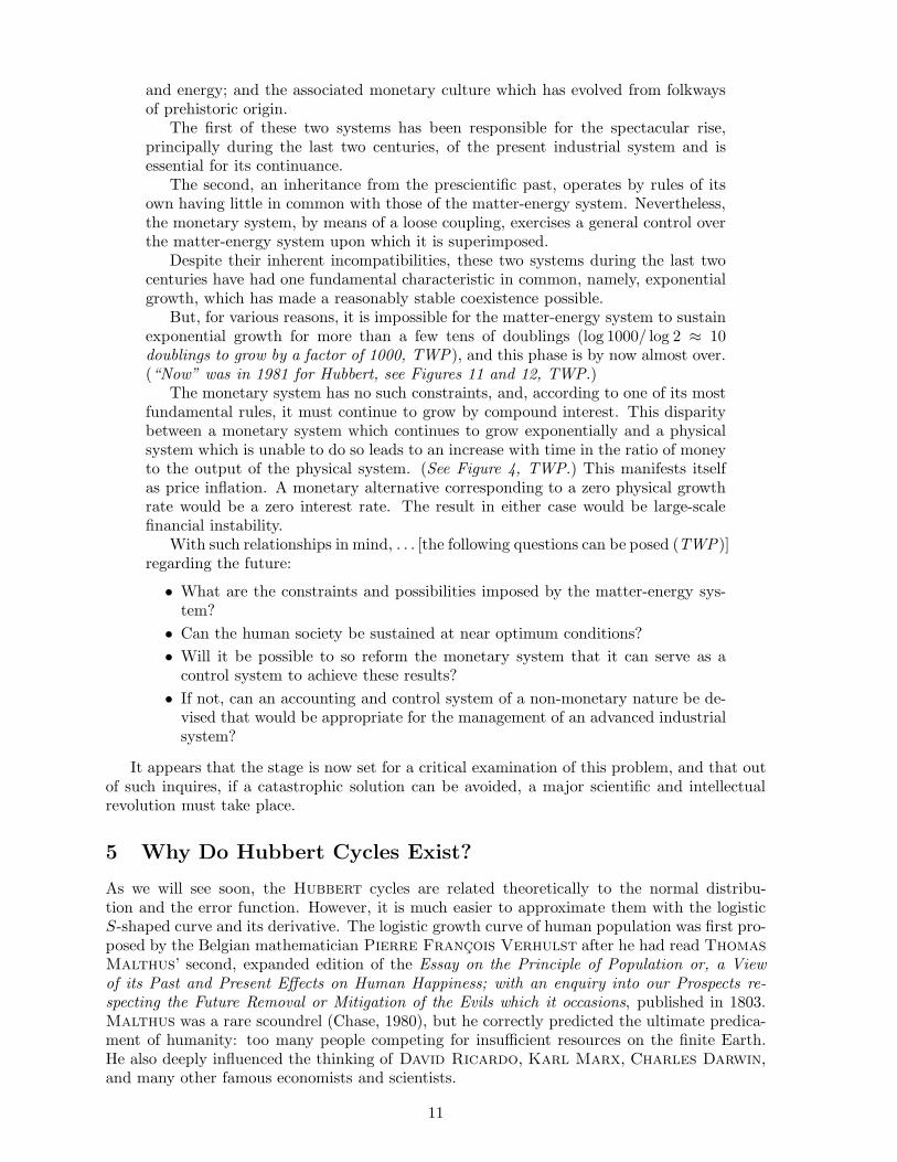
5 Why Do Hubbert Cycles Exist?

As we will see soon, the Hubbert cycles are related theoretically to the normal distribu-tion and the error function. However, it is much easier to approximate them with the logisticS-shaped curve and its derivative. The logistic growth curve of human population was first pro-posed by the Belgian mathematician Pierre Francois Verhulst after he had read ThomasMalthus’ second, expanded edition of the Essay on the Principle of Population or, a View

of its Past and Present Effects on Human Happiness; with an enquiry into our Prospects re-

specting the Future Removal or Mitigation of the Evils which it occasions, published in 1803.Malthus was a rare scoundrel (Chase, 1980), but he correctly predicted the ultimate predica-ment of humanity: too many people competing for insufficient resources on the finite Earth.He also deeply influenced the thinking of David Ricardo, Karl Marx, Charles Darwin,and many other famous economists and scientists.

11

Figure 14: Pierre Francois Verhulst, 1804 – 1849, Belgium.

5.1 Logistic Growth

The cumulative mass production or yield in logistic growth depends on time as follows (Verhulst,1838):

m(t) =mmax

1 + e−r(t−t∗)(1)

where mmax is the ultimate production or carrying capacity, r is the fractional rate of growth;t is time, and t∗ is the time of maximum production rate:

t∗ =1

rln

(

mmax

m(0)− 1

)

(2)

Remember that m(0) > 0!The production rate can be obtained by differentiation of the cumulative production m(t):

m =dm

dt=

2m∗

1 + cosh[r(t − t∗)](3)

where m∗ is the peak production rate.It may be easily shown that

mmax = 4m∗/r (4)

5.2 Logistic vs. Gaussian Distribution

The logistic equation (1) and its derivative, Eq. (2), are close (but not identical) to the Gaussiandistribution centered at t∗, and having the standard deviation, σ, related to r as follows:

σ ≈ 1.76275

r√

2 ln 2Matched half-widths (5)

or, better,

σ ≈ 4

r√

2πMatched peaks (6)

See Appendix B for the derivations.The cumulative logistic growth and its rate are then given by the following equations:

m(t) ≈ mmax

2

[

1 + erf(

(t − t∗)/√

2σ)]

(7)

12

where erf(x) = 2/√

π∫ x

0 e−t2dt is the error function

m = mmax1√2πσ

exp

[

−(t − t∗)2

2σ2

]

(8)

The two coefficients in bold rescale the normal distribution to the actual production history.

An argument advanced against Hubbert has been that the depletion histories of oil reser-voirs are distinctly skewed towards longer times. However, the Central Limit Theorem of statis-tics states (Davis, 1986) that if sets of random samples are taken from any population, thesample means will tend to be normally distributed. The tendency to normality becomes morepronounced for samples of larger size.

Alternatively, a Hubbert cycle may represent a normal process, e.g, (Ott, 1995). Manyvariables found in nature result from the summing of numerous unrelated components. Whenthe individual components are sufficiently unrelated and complex, the resulting sum tendstowards normality as the number of components comprising the sum becomes increasingly large.Two important conditions for a normal process are: (1) the summation of many continuousrandom variables, and (2) the independence of these random variables. A normal process isalso called a random-sum process (R− S-process).

In summary:

• We may think of all the oil (or gas) reservoirs as a very large statistical population char-acterized by the time-dependent, asymmetric distributions of every conceivable property.

• Throughout each year, we take a sample of the population by measuring the annualproduction qi from every reservoir in the population.

• We then sum up all the annual outputs of the reservoirs.

Sj =N

∑

i=1

qi(tj)

• This sum is proportional to the sample average for a given year

< qj >=1

N

N∑

i=1

qi(tj)

• The number of reservoirs in the sample should not change. As the reservoirs in the sampleare exhausted their production rates are set to zero.

• As we repeat this process over time, each year we get a set of < q(tj) >, j = 1, 2, . . . , NT .

• In effect, we sample different (time-dependent) distributions of properties of the underly-ing population and the distribution of the sample averages becomes approximately normal.

• We can repeat this procedure for each distinctly new population of reservoirs (multi-cycleanalysis). For example, in the US, the giant Proudhoe Bay field, or the Austin Chalkfields, or the offshore Gulf of Mexico fields, should form populations separate from thefundamental Hubbert cycle.

• By virtue of the future, unaccounted for reservoir populations, the Hubbert cycles of thecurrent populations will underestimate the ultimate world recovery.

13

1880 1900 1920 1940 1960 1980 2000 2020 2040 20600

5

10

15

20

25

30

Nat

ural

Gas

Pro

duct

ion,

EJ/

Yea

r

Actual productionHubbert cyclesSum of cycles

Figure 15: The Hubbert cycle analysis of natural gas endowment in the US. There are twomain cycles. The original Hubbert cycle for conventional natural gas peaked in 1972. Thesecond comparable cycle, resulting mostly from the Gulf of Mexico gas fields and unconventionalgas fields, had the highest associated drilling activity in 1981 and is peaking as of this writing.Since 1981, the majority of drilling for gas has occurred on land, more recently in unconventionalgas deposits in Texas, Colorado, New Mexico, Oklahoma, etc. Note that the production rateof natural gas in the US will be declining soon at 10-15% per year. The gas produced from thesecond main Hubbert cycle and the smaller cycles will be exhausted in the next 50 years. Therightmost small cycle is a hypothetical drawdown of the Prudhoe Bay and Thompson Point gascaps (1012 sm3 of natural gas) with the peak production rate in 2040. Data source: US DOEEIA.

We may also think about the U.S. annual oil production as of a random-sum process. Theannual production of each reservoir can be considered a random continuous variable. When wesum up the annual outputs of many reservoirs, we obtain a sum of the independent continuousrandom variables. This sum is normally distributed when we repeat the summation over manyyears.

In the U.S., there have been over 25 000 active oil fields, so the number of random variablesis very large. From one year to another, though, the underlying independent variables shouldnot become related because of artificial constraints, such as production curtailment caused byproration by the Texas Railroad Commission.

New oilfield discoveries and improved oil recovery methods introduce new random variables,which should be summed separately. This is the essence of “multi-Hubbert” cycle modeling.

In his fascinating paper (Laherrere, 1999), Jean H. Laherrere explains that many naturalprocesses may be modeled with multiple Hubbert cycles, each having a different peak andcentered at a different time. In the context of the oil industry, this corresponds to creating newsub-populations through new field discoveries or new oil recovery techniques. Laherrere callsthis approach the “multi-Hubbert” modeling.

6 US Natural Gas Production

A single Hubbert cycle has been used to model natural gas consumption in Poland (Siemeket al., 2003). In contrast, natural gas production in the US is a perfect example of two different

14

populations of gas-producing reservoirs. Between 1990 and 2007 gas production was 28% higher,see Figure 15, than the peak oil production between 1970 and 1983, see Figure 13. The earlynatural gas was associated with petroleum production and peaked in 1972, see the left mainHubbert cycle in Figure 15. This gas was mostly flared and the accounting of its volume wasinadequate at best. More recently, offshore gas/condensate reservoirs in the Gulf of Mexicoand unconventional gas deposits have dominated gas production in America, and are probablypeaking in 2008, see the right main Hubbert cycle in Figure 15 and the smaller cycles. Thesecond peak and the smaller Hubbert cycles have the increasing contributions from tight gassands and gas shales in the interior of the United States and coal-bed methane, see Figure 16.The second peak of gas production in the US has been flattened by a heroic drilling program,with 80% of all active rigs in the US drilling for gas, see Figure 17, and most gas rigs drillingthe unconventional deposits at an exponentially increasing cost, see Figure 18.

Remark 4 The current drilling effort in the US cannot be sustained without major new ad-vances to increase the productivity of tight gas formations. 2

The actual future course of US natural gas production will be the sum of known Hubbertcycles, shown in this paper, and future Hubbert cycles. The area under one future Hubbertcycle for natural gas is known today: Alaska. Published North Slope reserves of > 35 Tcf(trillion standard cubic feet) ≈ 1012 sm3 are proven6 in well-studied reservoirs (Prudhoe Bayand Point Thompson), so the actual resource is larger. Unfortunately, as Figure 15 attests, thedrawing down of gas caps at Prudhoe Bay and Point Thompson will have a relatively smallimpact on the overall availability of natural gas in the United States. According to my analysis,the remaining producible gas in the United States was 600 Tcf in 2007 and 700 Tcf in 2002,compared with 1100 – 1400 Tcf of technically recoverable gas estimated elsewhere7 in 2002.The other estimates include the yet-untapped volume of producible natural gas equal to 30 -40 times the known gas volume at Prudhoe Bay and Point Thompson. Fifty percent of thathypothetical producible gas volume has not yet been included in the current analysis.

7 Value of Technology

As shown in Figure 19, the difference between the actual oil production in the United Statesand the cumulative oil produced from the fundamental Hubbert cycle is at least 200 EJ, or twoyears of primary energy consumption in the US. This incremental oil has been – and will continueto be – produced mostly because of progress in the drilling and well completion technologies(better and faster drilling methods, directional wells, horizontal wells, multilateral wells, smartmulti-interval wells, etc.), fracturing technology, waterflood and polymer-enhanced waterflood,and enhanced oil recovery methods, mostly steam injection, but also CO2 injection. In naturalgas production, the impact of new technology to access unconventional gas resources has beenmore dramatic, more than doubling the ultimate recovery, see Figure 20. The differencebetween the cumulative gas production in 2060 and the fundamental gas cycle is 1000 EJ, or 10years of primary energy consumption in the US. In the United States, the impact of accessingnew gas resources and of new gas well technology is at least 5 times larger than that of newoil recovery technologies. More importantly, most new gas is produced by small independentcompanies, while the major oil companies have shown little interest.

6In Need of Access: Alaska’s Known and Potential Gas Resources, David Houseknecht, Research Geologist,

U.S. Geological Survey, Mark Myers, Director, Division of Oil and Gas, Dept. of Natural Resources, July 28,2004, lba.legis.state.ak.us/sga/0407281000.htm.

7See www.naturalgas.org/business/analysis.asp.

15

Figure 16: How is gas production kept relatively constant in the US? By drilling a myriadof deep expensive gas wells, some of which I photographed when flying over Colorado in thesummer of 2007. In 2006, ca. 1900 net (new - replacements) gas wells were drilled in the USeach month. Gas production from many of the new gas wells declines initially at 20 - 45% peryear in the first 1 – 2 years, stabilizing at a low rate later. Sources: Data from US DOE EIA;image by T. W. Patzek, 06/22/07.

1987 1993 1998 2004 20090

200

400

600

800

1000

1200

1400

1600

Rig

cou

nt

OilGas

Figure 17: The July 1987 – January 2008 count of US gas and oil rigs. Note that since the year1999 about 80% of all active rigs have drilled for gas. Data source: Baker-Hughes.

16

1960 1970 1980 1990 2000 2010 20200

0.5

1

1.5

2

2.5

3

3.5

4

4.5

5

Cos

t per

Gas

Wel

l, M

illio

ns C

onst

ant U

SD

Figure 18: Growth of gas well costs in constant dollars. In 2007 – 2008, the escalation of wellcosts was more than exponential. Data source: US DOE EIA.

1880 1900 1920 1940 1960 1980 2000 2020 2040 20600

200

400

600

800

1000

1200

1400

Cum

ulat

ive

Cru

de O

il P

rodu

ctio

n, E

J

400 years of ethanol

at 6G gal/yr

Figure 19: The cumulative oil production in the US cannot continue growing forever. Theincrement between the main Hubbert cycle recovery and the total recovery is equal to at leasttwice the total primary energy consumption in the USA in the year 2003. This difference is acontribution of new technology and research in the oil industry. Coincidentally, this differenceis equal to 400 years of pure ethanol production at 6 billion gallons per year, equal to the globalrecord set in the US in the year 2007. The small increase of the total recovery curve after 2030is caused by a hypothetical production of 7.7 billion barrels of oil from the Arctic NationalWildlife Refuge (ANWR) in Alaska.

8 Summary and Conclusions

In this paper I have shown that the rates of world and US oil production have doubled 10 times,each increasing by a factor of ca. 1000, before reaching their respective peaks. The peak ofUS oil production occurred in 1970 and global oil production probably peaked in 2005 – 2006.The natural gas production rate in America has also increased by a factor of 1000, and is at itssecond peak as of writing this paper in April 2008.

I have provided mathematical arguments for the existence of Hubbert cycles and their

17

practical equivalence to the logistic growth curves. The Hubbert cycle analysis of American oiland gas production has highlighted the existence of new populations of reservoirs, rather smallin the case of oil production, but very large in the case of gas production.

It turns out that improved technology and new science have allowed the American oil pro-ducers to increase their ultimate production by 2 years of total energy consumption in the US.The American gas producers, mostly small independents, will achieve an increase of ultimategas production larger than 10 years of total energy consumption in the US. Thus, the discountedcumulative value of good science and engineering in the American oil and gas industry is worthwell over 1 trillion US dollars in 2008, and it will continue to grow exponentially in the nearfuture, given the declining oil and gas production rates and the increasing real prices of bothcommodities.

The US and the world will have to come to grips with the obvious fact that the Earth isfinite and oil production will not be increasing any further. World gas production will continueto increase for some time, and then it will follow the oil production curve. The timing of thepeak of world gas production is difficult to pinpoint because of the generally poorer quality ofavailable data and the large gas resources that are still untapped.

An all-time record production of ethanol in the US in 2007 was a tiny and rather irrelevantaddition to the main energy supply schemes for humanity. To make things worse, this ethanol isproduced at high environmental and energy costs (Patzek, 2004; Patzek, 2006b; Patzek, 2006a;Patzek, 2007).

1880 1900 1920 1940 1960 1980 2000 2020 2040 20600

200

400

600

800

1000

1200

1400

1600

1800

2000

Cum

ulat

ive

Nat

ural

Gas

Pro

duct

ion,

EJ

Figure 20: The increment between the first main Hubbert cycle of natural gas production andthe ultimate total gas recovery is equal to 10 times the total US energy consumption in 2003.This difference is a contribution of new technology and research in the gas industry.

9 Acknowledgements

This paper has been written in memory of M. King Hubbert. His work, and the company heshaped, Shell Development, have had a significant impact on my professional interests and life.This paper draws from a Class Reader (and a future handbook) I have developed for a seniorundergraduate/graduate course, CE170, Earth, Humans, and Energy. I taught CE170 at UCBerkeley in Spring of 2007. I have received no financial support for this work.

I would like to thank Mr. Greg Croft of Greg Croft, Inc., for his numerous inputs andcritical review of the manuscript. I would also like to thank my son, Lucas, for editing thepaper and improving its readability.

18

References

Anonymous 1995a, Energy Balances of OECD Countries 1992-1993, Report OECD, Organi-zation for Economic Co-operation and Development, International Energy Agency, Paris.

Anonymous 1995b, International Energy Annual 1993, Report DOE/EIA-0219(93), U.S. De-partment of Energy, Washington, D.C..

Attanasi, E. D. 2005, Undiscovered oil resources in the Federal portion of the 1002 Area of

the Arctic National Wildlife Refuge: An economic update, Open-File Report 1217, U.S.Department of the Interior U.S. Geological Survey U.S. Geological Survey, Reston, Virginia.

Bossel, U. 2003, Well-to-Wheel Studies, Heating Values, and the Energy Conservation Prin-

ciple, Report E10, European Fuel Cell Forum, Oberrohrdorf, Switzerland, Posted atwww.efcf.com/reports.

Chase, A. 1980, The Legacy of Malthus – The Social Costs of the New Scientific Racism,University if Illinois Press, Urbana, IL.

Daly, H. E. 1977, Steady-State Economics, W. H. Freeman and Company, San Francisco.Davis, J. C. 1986, Statistics and Data Analysis in Geology, John Wiley & Sons, New York, 2nd

edition.Ellis, R. 1991, Men & Whales, The Lyons Press, New York.Foss, M. M. 2004, Interstate natural gas-quality specifications & interchangeability, Report,

Bureau of Economic Geology – Center for Energy Economics, Highway 6, Suite 300, SugarLand, Texas 77478, www.beg.utexas.edu/energyecon/lng.

Georgescu-Roegen, N. 1971, The Entropy Law and the Economic Process, Harvard UniversityPress, Cambridge, Massachusetts.

Hubbert, M. K. 1949, Energy from fossil fuels, Science 109(2823): 103–109.Hubbert, M. K. 1956, Nuclear Energy and the Fossil Fuels, Presentation at the Spring Meeting

of the Southern District Division of the American Petroleum Institute, Shell DevelopmentCompany, San Antonio, TX, http://www.hubbertpeak.com/hubbert/1956/1956.pdf.

Laherrere, J. H. 1999, What goes up must come down, but when will it peak?, O&GJ (Feb.1): 57–64.

Odum, E. 1998, Ecological Vignettes – Ecological Approaches to Dealing with Human Predica-

ments, Hardwood Academic Publishers, Amsterdam.Ott, W. R. 1995, Environmental Statistics and Data analysis, Lewis Publishers, Boca Raton.Patzek, T. W. 2004, Thermodynamics of the corn-ethanol biofuel cycle, Critical Re-

views in Plant Sciences 23(6): 519–567, An updated web version is at http://-petroleum.berkeley.edu/papers/patzek/CRPS416-Patzek-Web.pdf.

Patzek, T. W. 2006a, A First-Law Thermodynamic Analysis of the Corn-Ethanol Cycle, Natural

Resources Research 15(4): 255 – 270.Patzek, T. W. 2006b, Letter, Science 312(5781): 1747.Patzek, T. W. 2007, How can we outlive our way of life?, in 20th Round Table on Sus-

tainable Development of Biofuels: Is the Cure Worse than the Disease?, OECD, Paris,www.oecd.org/dataoecd/2/61/40225820.pdf.

Patzek, T. W. and Pimentel, D. 2006, Thermodynamics of energy production frombiomass, Critical Reviews in Plant Sciences 24(5–6): 329–364, Available at http://-petroleum.berkeley.edu/papers/patzek/CRPS-BiomassPaper.pdf.

Siemek, J., Nagy, S., and Rychlicki, S. 2003, Estimation of natural-gas consumption in Polandbased on the logistic-curve interpretation, Applied Energy 75: 1 – 7.

Szargut, J., Morris, D. R., and Steward, F. R. 1988, Exergy analysis of thermal and metallurgical

processes, Hemisphere Publishing Corporation, New York.Verhulst, P. F. 1838, Notice sur la loi que la population suit dans son accroissement, Corr.

Math. et Phys. publ. par A. Quetelet T. X. (also numbered T. II of the third series):113–121.

19

A Units and Conversions

The fundamental unit of energy used in this paper is 1 exajoule (EJ) or 1018 J. This amountof energy in food, when digested, feeds the entire population of the United States, 303 millionpeople, for one year (Patzek, 2007). Currently the US uses about 105 EJ per year as primaryenergy (Patzek, 2007). The world uses about 4 times more primary energy, ca. 420 EJ peryear (IEA). All comparisons are made using the higher heating values of fuels, the only sensiblechoice for fuels with different hydrogen and oxygen contents (Bossel, 2003).

One metric tonne of oil equivalent (toe) is a unit for measuring heating value of crude oil.Since there are different definitions in the literature, the IEA/OECD definition is adopted: 1toe equals 10 Gcal (thermochemical) or 41.868 GJ or 5.80 MBtu/bbl (Anonymous, 1995a). Itis the standard amount of heat that would be produced by burning one metric ton of crudeoil, presumably its lower heating value LHV. The higher heating value HHV of oil equivalent isobtained by increasing the LHV value by 7% (Szargut et al., 1988). Since different crudes differin chemical composition and generate varying amounts of heat when burnt, the toe energy unitis a convention. The heat content of crude oil from different countries varies from about 5.6MBtu per barrel to about 6.3 MBtu (Anonymous, 1995b), with the arithmetic mean of 5.8 MBtuper barrel.

The reported thousands of barrels of oil produced per day (BOPD) are converted to EJ yr−1

in the following way

EJ yr−1 = 1000 BOPD × 1000 × 365 × 134 × 44.8 × 106/1018 (9)

where 134 kg/bbl is the assumed average mass of 1 barrel of world oil, whose equivalent higherheating value is 44.8 × 106 J/kg.

The US crude oil production was reported by US DOE EIA in mega British thermal units(1 MBtu = 1055.056 MJ)) per year until 2005, and then switched back to 1000 BOPD. I haveused the 2005 production to convert from BOPD to MBtu/yr, and to EJ/yr. Thus calculatedenergy of US petroleum production is probably the lower heating value.

To convert mega standard cubic feet (Mscf) of natural gas per year to EJ yr−1 the followingformula has been used

EJ yr−1 = Mscf/yr × 106 × 1050 × 1055.056/1018 (10)

where 1050 Btu/scf is the assumed average HHV of natural gas in the US (Foss, 2004).

B Matching the Logistic and Normal Distributions

To approximate the Gaussian distribution (rate) curve,

f1(t;σ, t∗,mmax) = mmax1√2πσ

exp

[

−(t − t∗)2

2σ2

]

(11)

with the logistic curve,

f2(t; r, t∗,mmax) =

mmaxr

2

1

1 + cosh[r(t − t∗)](12)

we will first attempt to match their full widths at 1/2 heights.For the Gaussian distribution

f1(t0;σ, t∗,mmax) =1

2f1(t

∗;σ, t∗,mmax)

1√2πσ

exp

[

−(t0 − t∗)2

2σ2

]

=1

2

1√2πσ

exp

[

−(t0 − t∗)2

2σ2

]

=1

2

(13)

20

−10 −5 0 5 100

0.05

0.1

0.15

0.2

0.25

LogisticGauss

Figure 21: Logistic vs. normal distribution with matched half-widths, for r = 1, t∗ = 0,m∗ = 1/4.

and

(t0 − t∗)2

2σ2= ln 2

t0 = ±σ√

2 ln 2 + t∗(14)

The full width at half maximum is therefore

2σ√

2 ln 2

for the Gaussian distribution.For the logistic distribution

f2(t0; r, t∗,mmax) =

1

2f2(t

∗; r, t∗,mmax)

mmaxr

2

1

1 + cosh[r(t0 − t∗)]=

mmaxr

8

1

1 + cosh[r(t0 − t∗)]=

1

4

cosh[r(t0 − t∗)] = 3

(15)

An approximate solution to this transcendental equation is r(t0− t∗) ≈ 1.76275. The full widthat half maximum is therefore

3.5255

rfor the logistic distribution.

To match the respective full widths, we require that

2σ√

2 ln 2 =3.5255

r

σ =1.76275

r√

2 ln 2

(16)

To match the peaks, we require that

mmax√2πσ

=rmmax

4

σ =4

r√

2π

(17)

21

Since heights of the two distributions are somewhat different for equal half-widths (the t0 inEq. (15)4 is in fact different than that in Eq. (13)3), the half-width match is approximate, seeFigure 21. The peak matching is also approximate, see Figure 22, but seems to be better.

−10 −5 0 5 100

0.05

0.1

0.15

0.2

0.25

LogisticGauss

Figure 22: Logistic vs. normal distribution with matched half-peaks, for r = 1, t∗ = 0,m∗ = 1/4.

22