Exploring the validation of lanchester equations for the ... · EXPLORING THE VALIDATION OF...

Calhoun: The NPS Institutional Archive

Theses and Dissertations Thesis Collection

2001-06

Exploring the validation of lanchester equations for

the Battle of Kursk

Dinges, John A.

Monterey, California. Naval Postgraduate School

http://hdl.handle.net/10945/2540

NAVAL POSTGRADUATE SCHOOL Monterey, California

THESIS

Approved for public release; distribution is unlimited.

EXPLORING THE VALIDATION OF LANCHESTER EQUATIONS FOR THE BATTLE OF KURSK

by

John A. Dinges

June 2001

Thesis Advisor: Thomas W. Lucas Second Reader: Eugene P. Paulo


John A. Dinges-Captain, United States Army B.S., United States Military Academy, 1991

Master of Science in Operations Research-June 2001 Advisor: Thomas W. Lucas, Department of Operations Research

Second Reader: Eugene P. Paulo, Department of Operations Research

This thesis explores the validation of Lanchester equations as models of the attrition process for the Battle of Kursk in World War II. The methodology and results of this study extend previous validation efforts undertaken since the development of the Ardennes Campaign Simulation Data Base (ACSDB) in 1989 and the Kursk Data Base (KDB) in 1996. The KDB is a computerized database developed by the Dupuy Institute and the Center for Army Analysis from military archives in Germany and Russia. The data are two-sided, time-phased (daily), highly detailed, and encompass 15 days of the campaign. The primary areas of analysis are the effect of using purely engaged forces in parameter estimation and the effect of force weighting in forming homogeneous force strengths. Based on the numbers of personnel, tanks, armored personnel carriers, and artillery, three different data sets were constructed: all combat forces in the campaign, combat forces within contact that are both engaged and not engaged, and combat forces within contact that are engaged. In addition, a weight optimization program using a steepest ascent algorithm was developed and utilized. Findings indicate that Lanchester-based models provide a considerably better fit for data sets composed only of forces that are actively engaged. Also, Lanchester’s linear model appears to provide the best fit to the Battle of Kursk data. Finally, optimization of force weights does not significantly improve the fit of Lanchester models.

DoD KEY TECHNOLOGY AREA: Modeling and Simulation KEYWORDS: Lanchester Equations, Battle of Kursk, Combat Models, Attrition, Model Validation

i

REPORT DOCUMENTATION PAGE Form Approved OMB No. 0704-0188 Public reporting burden for this collection of information is estimated to average 1 hour per response, including the time for reviewing instruction, searching existing data sources, gathering and maintaining the data needed, and completing and reviewing the collection of information. Send comments regarding this burden estimate or any other aspect of this collection of information, including suggestions for reducing this burden, to Washington headquarters Services, Directorate for Information Operations and Reports, 1215 Jefferson Davis Highway, Suite 1204, Arlington, VA 22202-4302, and to the Office of Management and Budget, Paperwork Reduction Project (0704-0188) Washington DC 20503. 1. AGENCY USE ONLY (Leave blank)

2. REPORT DATE June 2001

3. REPORT TYPE AND DATES COVERED Master’s Thesis

4. TITLE AND SUBTITLE: Title (Mix case letters) Exploring the Validation of Lanchester Equations for the Battle of Kursk 6. AUTHOR(S) John A. Dinges

5. FUNDING NUMBERS

7. PERFORMING ORGANIZATION NAME(S) AND ADDRESS(ES) Naval Postgraduate School Monterey, CA 93943-5000

8. PERFORMING ORGANIZATION REPORT NUMBER

9. SPONSORING / MONITORING AGENCY NAME(S) AND ADDRESS(ES) N/A

10. SPONSORING / MONITORING AGENCY REPORT NUMBER

11. SUPPLEMENTARY NOTES The views expressed in this thesis are those of the author and do not reflect the official policy or position of the Department of Defense or the U.S. Government. 12a. DISTRIBUTION / AVAILABILITY STATEMENT Approved for public release; distribution is unlimited.

12b. DISTRIBUTION CODE

13. ABSTRACT (maximum 200 words) This thesis explores the validation of Lanchester equations as models of the attrition process for the Battle of Kursk in World War II. The methodology and results of this study extend previous validation efforts undertaken since the development of the Ardennes Campaign Simulation Data Base (ACSDB) in 1989 and the Kursk Data Base (KDB) in 1996. The KDB is a computerized database developed by the Dupuy Institute and the Center for Army Analysis from military archives in Germany and Russia. The data are two-sided, time -phased (daily), highly detailed, and encompass 15 days of the campaign. The primary areas of analysis are the effect of using purely engaged forces in parameter estimation and the effect of force weighting in forming homogeneous force strengths. Based on the numbers of personnel, tanks, armored personnel carriers, and artillery, three different data sets were constructed: all combat forces in the campaign, combat forces within contact that are both engaged and not engaged, and combat forces within contact that are engaged. In addition, a weight optimization program using a steepest ascent algorithm was developed and utilized. Findings indicate that Lanchester-based models provide a considerably better fit for data sets composed only of forces that are actively engaged. Also, Lanchester’s linear model appears to provide the best fit to the Battle of Kursk data. Finally, optimization of force weights does not significantly improve the fit of Lanchester models.

15. NUMBER OF PAGES

14. SUBJECT TERMS Combat Modeling, Lanchester Equations, Battle of Kursk

16. PRICE CODE

17. SECURITY CLASSIFICATION OF REPORT

Unclassified

18. SECURITY CLASSIFICATION OF THIS PAGE

Unclassified

19. SECURITY CLASSIFICATION OF ABSTRACT

Unclassified

20. LIMITATION OF ABSTRACT

UL

NSN 7540-01-280-5500 Standard Form 298 (Rev. 2-89) Prescribed by ANSI Std. 239-18

ii

THIS PAGE INTENTIONALLY LEFT BLANK

iii

Approved for public release; distribution is unlimited.


John A. Dinges

Captain, United States Army B.S., United States Military Academy, 1991

Submitted in partial fulfillment of the requirements for the degree of

MASTER OF SCIENCE IN OPERATIONS RESEARCH

from the

NAVAL POSTGRADUATE SCHOOL June 2001

Author: ___________________________________________ John A. Dinges

Approved by: ___________________________________________ Thomas W. Lucas, Thesis Advisor

___________________________________________ Eugene P. Paulo, Second Reader

___________________________________________ James N. Eagle, Chairman

Department of Operations Research

iv


v

ABSTRACT

This thesis explores the validation of Lanchester equations as models of the

attrition process for the Battle of Kursk in World War II. The methodology and results of

this study extend previous validation efforts undertaken since the development of the

Ardennes Campaign Simulation Data Base (ACSDB) in 1989 and the Kursk Data Base

(KDB) in 1996. The KDB is a computerized database developed by the Dupuy Institute

and the Center for Army Analysis from military archives in Germany and Russia. The

data are two-sided, time-phased (daily), highly detailed, and encompass 15 days of the

campaign. The primary areas of analysis are the effect of using purely engaged forces in

parameter estimation and the effect of force weighting in forming homogeneous force

strengths. Based on the numbers of personnel, tanks, armored personnel carriers, and

artillery, three different data sets were constructed: all combat forces in the campaign,

combat forces within contact that are both engaged and not engaged, and combat forces

within contact that are engaged. In addition, a weight optimization program using a

steepest ascent algorithm was developed and utilized. Findings indicate that Lanchester-

based models provide a considerably better fit for data sets composed only of forces that

are actively engaged. Also, Lanchester’s linear model appears to provide the best fit to

the Battle of Kursk data. Finally, optimization of force weights does not significantly

improve the fit of Lanchester models.

vi


vii

TABLE OF CONTENTS

I. INTRODUCTION........................................................................................................1 A. OVERVIEW.....................................................................................................1 B. BACKGROUND ..............................................................................................2

1. Lanchester Equations ..........................................................................2 2. Previous Studies ...................................................................................3

a. Engel’s Study.............................................................................4 b. Hartley and Helmbold’s Study .................................................4 c. Bracken’s Study ........................................................................5 d. Fricker’s Study..........................................................................5 e. Turkes’ Study ............................................................................6

3. Areas of Interest Not Addressed in Previous Studies.......................7 a. Engagement Levels of Forces...................................................7 b. Weighting of Individual Weapon Types...................................7

C. OBJECTIVE ....................................................................................................8 1. Stated Objectives..................................................................................8 2. Measures of Performance....................................................................9

D. METHODOLOGY AND ORGANIZATION................................................9

II. HISTORICAL OVERVIEW AND DATA SUMMARY........................................11 A. HISTORICAL OVERVIEW OF THE BATTLE OF KURSK .................11 B. DATA SUMMARY........................................................................................13

1. Description of Kursk Database.........................................................13 2. Database Formulation .......................................................................14

a. Manpower ................................................................................15 b. Weapons Classification...........................................................15 c. ACUD, CCUD, and FCUD Data...........................................17

3. Combat Postures ................................................................................20 4. Correlation Analysis ..........................................................................21

III. EXPLORATION OF DATA SETS AND WEIGHTING METHODOLOGIES .................................................................................................27 A. COMPARATIVE ANALYSIS OF PREVIOUS METHODOLOGIES ....27

1. Bracken Methodology........................................................................27 a. Summary..................................................................................27 b. Aggregation of Data................................................................30 c. Application of Methodology to ACUD, CCUD, FCUD

Data..........................................................................................31 d. Results......................................................................................32

2. Turkes Methodology ..........................................................................34 a. Summary..................................................................................34 b. Application of Methodology to ACUD, CCUD, FCUD

Data..........................................................................................35

viii

c. Results......................................................................................36 d. p and q Constrained to Linear, Square, and Logarithmic

Models......................................................................................41 e. Model of Manpower Only.......................................................43 f. Accuracy of Logarithmically Transformed Linear

Regression ...............................................................................44 B. WEIGHT OPTIMALITY.............................................................................48

1. Methodology .......................................................................................48 a. Objective Function..................................................................48 b. Theoretical Summary..............................................................49 c. Description of Algorithm........................................................51

2. Results .................................................................................................54 a. Unconstrained p and q ..................................................................54 b. p and q Constrained to Linear, Square, and Logarithmic

Models......................................................................................56 c. Application of Model to Ardennes Campaign Data

(ACUD Only)...........................................................................59

IV. CONCLUSIONS AND RECOMMENDATIONS...................................................61 A. CONCLUSIONS ............................................................................................61

1. Data Correlations May Reflect Lanchester Models .......................61 2. Lanchester Models More Accurately Fit FCUD Data....................61 3. FCUD Data Reveals Important Insight Concerning the Battle

of Kursk ..............................................................................................62 4. Transformed Linear Regression Fails to Optimize p, q, a, and b

in All Cases .........................................................................................62 5. Weight Optimization Does Not Greatly Affect the Fit of

Lanchester Models .............................................................................63 6. Optimized Weights FOR CCUD and FCUD Data Do Reflect

Historical Accounts of the Battle of Kursk......................................63 7. The Battle of Kursk Most Resembles the Lanchester Linear

Model for the FCUD Data Set...........................................................64 B. RECOMMENDATIONS FOR FURTHER RESEARCH .........................65

1. Extended Analysis Required for ACUD, CCUD, and FCUD Data Sets..............................................................................................65

2. Alternate Methods Required for Optimizing p, q, a, and b............65

APPENDIX A. WEIGHT OPTIMIZATION PROGRAM (UNCONSTRAINED)................................................................................................67

APPENDIX B. WEIGHT OPTIMIZATION PROGRAM (CONSTRAINED TO POSITIVE WEIGHTS) ......................................................................................71

LIST OF REFERENCES ......................................................................................................95

INITIAL DISTRIBUTION LIST.........................................................................................97

ix

LIST OF FIGURES

Figure I.1. Contour Filled Plot Of SSR Values For Battle of Kursk. ..................................7 Figure II.1. Operation Citadel (July 4 – 12)........................................................................12 Figure II.2. German vs. Soviet Manpower..........................................................................18 Figure II.3. German vs. Soviet Tanks. ................................................................................19 Figure II.4. German vs. Soviet APCs..................................................................................19 Figure II.5. German vs. Soviet Artillery.. ...........................................................................20 Figure II.6. Pair-Wise Scatter Plot Of Soviet Losses (SL), German Losses (GL),

German On-Hand (G), and Soviet On-Hand (S) From ACUD Data Set. ........23 Figure II.7. Pair-Wise Scatter plot Of Soviet Losses (SL), German Losses (GL),

German On-Hand (G), and Soviet On-Hand (S) From CCUD Data Set. ........24 Figure II.8. Pair-Wise Scatter Plot Of Soviet Losses (SL), German Losses (GL),

German On-Hand (G), and Soviet On-Hand (S) From FCUD Data Set. ........25 Figure III.1. Fitted Versus Real German Casualties For ACUD Data Set.. .........................38 Figure III.2. Fitted Versus Real Soviet Casualties For ACUD Data Set..............................38 Figure III.3. Fitted Versus Real German Casualties For CCUD Data Set. ..........................39 Figure III.4. Fitted Versus Real Soviet Casualties For CCUD Data Set. .............................39 Figure III.5. Fitted Versus Real German Casualties For FCUD Data Set............................40 Figure III.6. Fitted Versus Real Soviet Casualties For FCUD Data Set. .............................40 Figure III.7. Contour Plot Of R2 Surface For ACUD Data Set With Bracken Weights. .....46 Figure III.8. Contour Plot Of R2 Surface For CCUD Data Set With Bracken Weights.. .....47 Figure III.9. Contour Plot Of R2 Surface For FCUD Data Set With Bracken Weights........47 Figure III.10. Flowchart Depicting the Weight Optimization Algorithm. .............................53 Figure III.11. Fitted Versus Real German Casualties For FCUD Data Set Using the

Linear Model....................................................................................................57 Figure III.12. Fitted Versus Real Soviet Casualties For FCUD Data Set Using the Linear

Model. ..............................................................................................................58 Figure IV.1. Contour Plot Of R2 Surface For FCUD Data Set With All Force Weights

Equal To One.. .................................................................................................64

x


xi

LIST OF TABLES

Table II.1. Summary Of German and Soviet Weapons Types Within Tanks, APC, and Artillery Classification. ....................................................................................16

Table II.2. German and Soviet ACUD Data. .....................................................................17 Table II.3. German and Soviet CCUD Data. ....................................................................17 Table II.4. German and Soviet FCUD Data. .....................................................................18 Table II.5. Correlation matrix of ACUD Data...................................................................23 Table II.6. Correlation matrix of CCUD Data. ..................................................................24 Table II.7. Correlation matrix of FCUD Data. ..................................................................25 Table III.1. Resulting Parameters Of Bracken’s Analysis Of the Ardennes Campaign

Data. .................................................................................................................29 Table III.2. Aggregated Data For German Forces. .............................................................30 Table III.3. Aggregated Data For Soviet Forces. ................................................................31 Table III.4. Results Of Bracken's Method When Applied To Model 1. .............................32 Table III.5. Results Of Bracken's Method When Applied To Model 3. .............................33 Table III.6. Resulting Parameters Of Turkes’ Linear Regression Analysis Of the Battle

Of Kursk...........................................................................................................35 Table III.7. Results Of Linear Regression When Applied To ACUD, CCUD, and

FCUD Data Sets...............................................................................................36 Table III.8. Linear Regression Results For FCUD Data With p and q Restricted To

Lanchester Linear, Square, and Logarithmic Models. .....................................42 Table III.9. Linear Regression Results For CCUD Data With p and q Restricted To

Lanchester Linear, Square, and Logarithmic Models. .....................................43 Table III.10. Linear Regression Results For ACUD Data With p and q Restricted To

Lanchester Linear, Square, and Logarithmic models. .....................................43 Table III.11. Linear Regression Results For Manpower Only..............................................44 Table III.12. Results Of Combinatoric Search Over p and q Using Bracken’s Weighting

Criteria. ............................................................................................................45 Table III.13. Weight Optimization Results For the Battle Of Kursk Data. ..........................54 Table III.14. Weight Optimization Results For FCUD Data With p and q Restricted To

Lanchester Linear, Square, and Logarithmic Models. .....................................56 Table III.15. Weight Optimization Results For CCUD Data With p and q Restricted To

Lanchester Linear, Square, and Logarithmic Models. .....................................56 Table III.16. Weight Optimization Results For ACUD Data With p and q Restricted To

Lanchester Linear, Square, and Logarithmic Models. .....................................56 Table III.17. Results Of Ardennes Campaign Analysis. .......................................................59

xii


xiii

LIST OF SYMBOLS, ACRONYMS AND ABBREVIATIONS

• ACSDB: Ardennes Campaign Simulation Data Base

• ACUD: All Combat Unit Data

• APC: Armored Personnel Carrier

• ARCAS: The Ardennes Campaign Simulation Study

• CAA: US Army Concepts Analysis Agency

• CCUD: Contact Combat Unit Data

• FCUD: Fighting Combat Unit Data

• G: German forces on hand

• GL: German losses

• KDB: Kursk Data Base

• KOSAVE II: The Kursk Operation Simulation and Validation Exercise (Phase II)

• OH: On hand

• S: Soviet forces on hand

• SL: Soviet losses

• SSR: Sum of Squared Residuals

xiv


xv

ACKNOWLEDGMENTS

The author wishes to thank Professor Lucas for his immeasurable guidance during

the preparation of this thesis. His expert vision and recommendations were vital

throughout the analysis process, and his extensive knowledge of the subject area was an

extremely useful resource. In addition, LTC Paulo provided invaluable assistance in the

editing process, and his recommendations resulted in a better final product. Finally, the

previous theses of LT Turkes and LT Gozel provided an outstanding framework for the

analysis of the Battle of Kursk data. In particular, LT Gozel’s use of alternate data sets

was helpful in the preparation of the data sets used in this thesis.

xvi


xvii

EXECUTIVE SUMMARY

Since the dramatic growth of operations research during and after World War II,

modeling of combat at both the tactical and strategic level has grown dramatically. One

complicated characteristic of most combat models is the representation of the decrease in

force levels over time, commonly referred to as attrition. In an effort to accurately model

the attrition process, many combat models employ Lanchester-type equations.

Fortunately, the development of the Ardennes Campaign Simulation Data Base (ACSDB)

in 1989 and the Kursk Data Base (KDB) in 1996 has enabled more analysis concerning

the empirical validation of Lanchester equations. The purpose of this study is to explore

the validation of Lanchester equations as they model the attrition process of the Battle of

Kursk in World War II. In particular, this thesis focuses on the effect of using purely

engaged forces in parameter estimation and the effect of force weighting in forming

homogeneous force strengths.

The general form of the Lanchester model is:

B& (t) = aR(t)

pB(t)q,

R& (t) = bB(t)

pR(t)q,

where B(t) and R(t) are the strengths of blue and red forces at time t, B& (t) and R& (t) are the

rates at which blue forces and red forces are killed at time t, a and b are attrition

parameters, p is the exponent parameter of the attacking force, and q is the exponent

parameter of the defending force. Three specific variations of these equations are of

particular interest due to their simplicity and intuitive results. First, the Lanchester linear

model exists when p = q = 1. In this case, the casualty rate of a force is proportional to

xviii

the product of its force size and the enemy’s force size. Next, the Lanchester square

model exists when p = 1 and q = 0. Here, the casualty rate of a force is proportional only

to the enemy force size. Finally, the logarithmic model exists when p = 0 and q = 1 and

describes a situation when the casualty rate is only proportional to one’s own force size

and not the enemy’s.

In previous studies concerning the validation of Lanchester equations with

historical data, the authors make no distinction between those forces that are actually

engaged and those that are not engaged. However, the KDB does delineate between all

combat units, all combat units within contact but not engaged, and all combat units within

contact and engaged. Quite possibly, Lanchester equations may prove more applicable to

one of these data types than the others. This result could prove useful in determining

how combat simulations that use Lanchester-based equations are best utilized.

In order to conduct this analysis, three separate data sets were constructed from

the KDB. These data sets divide the KDB into three inclusive categories: all combat unit

data (ACUD), combat unit data for those units that are within contact (CCUD), and

combat unit data for only those units that are actually fighting (FCUD). Each of these

data sets was analyzed using three different techniques. The first two techniques consist

of the application of previous methodologies used by Bracken [Ref. 4] in his analysis of

the Ardennes Campaign and by Turkes [Ref. 2] in his analysis of the Battle of Kursk.

Bracken’s technique involved delineating a range of values for each parameter and

searching on a discrete grid over this range for the set of parameters resulting in lowest

sum of squared residuals when compared to the actual data. Turkes modeled his

technique after a method developed by Fricker. [Ref. 5] This process consists of using

xix

linear regression on logarithmically transformed data to estimate the unknown

parameters. Each of these models was applied to the ACUD, CCUD, and FCUD data

sets to determine which set resulted in a better fit.

The final area of analysis explores the area of force weighting and its affect on a

model’s fit. Force weighting is often utilized to combine differing force types into a

homogeneous force level. This is accomplished by multiplying the actual size of each

force type by an appropriate weighting parameter and summing for each day. In this

analysis, personnel, tanks, armored personnel carriers, and artillery were combined to

produce a homogeneous level of force strength. However, no common methodology or

rigorous criteria exists for determining the weighting parameters of each force type. The

selection of these weights may actually have a considerable impact on the model’s fit to

the actual data.

In order to determine the ideal weights, a weight optimization algorithm was

developed and applied to each of the three data sets. This algorithm consists of a steepest

ascent search combined with linear regression on the logarithmically transformed

variables to determine the weights that result in the best fit of the model. This procedure

was also applied to Lanchester’s square, linear, and logarithmic models, as well as to the

ACUD data from the Ardennes campaign.

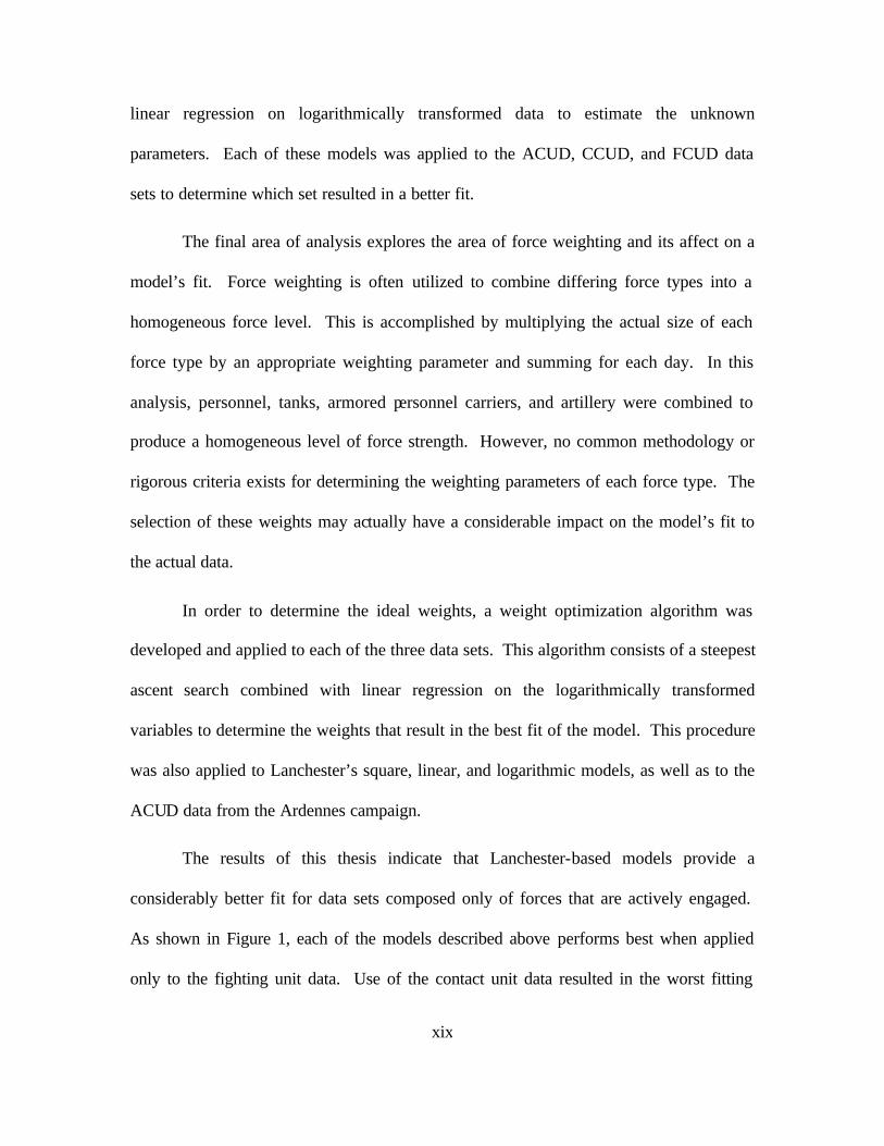
The results of this thesis indicate that Lanchester-based models provide a

considerably better fit for data sets composed only of forces that are actively engaged.

As shown in Figure 1, each of the models described above performs best when applied

only to the fighting unit data. Use of the contact unit data resulted in the worst fitting

xx

model. This result suggests that Lanchester-type models more accurately predict combat

losses in cases where only fully engaged forces are considered.

R-Squared Comparison

-0.1

0

0.10.2

0.3

0.4

0.5

0.6

0.7

Bracken Method Turkes Method Optimized Weights

Model Type

R-S

quar

ed

All UnitsContact UnitsFighting Units

Figure 1. Comparison of R2 values for three separate models. A higher R2 value indicates a better fit to the actual data.

Another significant finding resulted from the direct application of Lanchester’s

square, linear, and logarithmic equations. Of all models investigated in this thesis,

Lanchester’s linear model provides the best fit to the Battle of Kursk data. This is a

significant finding and represents one of the few cases in which one of Lanchester’s basic

models was found to apply to an actual battle using highly aggregated data. This implies

that a force’s casualties were a function of both friendly and enemy force levels for

engaged forces during the Battle of Kursk. The resulting parameters and R2 values for

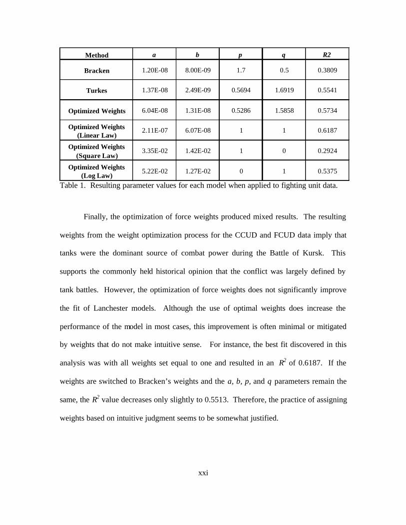
each model when applied to the fighting unit data are shown in Table 1. As noted earlier,

use of the fighting unit data resulted in the best fit for each model.

xxi

Method a b p q R2

Bracken 1.20E-08 8.00E-09 1.7 0.5 0.3809

Turkes 1.37E-08 2.49E-09 0.5694 1.6919 0.5541

Optimized Weights 6.04E-08 1.31E-08 0.5286 1.5858 0.5734

Optimized Weights (Linear Law)

2.11E-07 6.07E-08 1 1 0.6187

Optimized Weights (Square Law)

3.35E-02 1.42E-02 1 0 0.2924

Optimized Weights (Log Law)

5.22E-02 1.27E-02 0 1 0.5375

Table 1. Resulting parameter values for each model when applied to fighting unit data.

Finally, the optimization of force weights produced mixed results. The resulting

weights from the weight optimization process for the CCUD and FCUD data imply that

tanks were the dominant source of combat power during the Battle of Kursk. This

supports the commonly held historical opinion that the conflict was largely defined by

tank battles. However, the optimization of force weights does not significantly improve

the fit of Lanchester models. Although the use of optimal weights does increase the

performance of the model in most cases, this improvement is often minimal or mitigated

by weights that do not make intuitive sense. For instance, the best fit discovered in this

analysis was with all weights set equal to one and resulted in an R2 of 0.6187. If the

weights are switched to Bracken’s weights and the a, b, p, and q parameters remain the

same, the R2 value decreases only slightly to 0.5513. Therefore, the practice of assigning

weights based on intuitive judgment seems to be somewhat justified.

xxii


1

I. INTRODUCTION

A. OVERVIEW

Since the dramatic growth of operations research during and after World War II,

the United States military has used various forms of modeling to study complex

processes. In particular, modeling of combat at both the tactical and strategic level has

grown dramatically with the advent of increased computing power. One complicated

characteristic of most combat models is the representation of the decrease in force levels

over time, commonly referred to as attrition. In an effort to accurately model the attrition

process, many combat models employ Lanchester-type equations. However, due to a

serious deficiency in the quality of historical data, empirical validation of Lanchester

equations in modeling attrition has been sorely lacking. Fortunately, the development of

the Ardennes Campaign Simulation Data Base (ACSDB) in 1989 and the Kursk Data

Base (KDB) in 1996 has enabled more analysis in this area. The purpose of this study is

to explore the validation of Lanchester equations as they model the attrition process of

the Battle of Kursk in World War II. In particular, this thesis focuses on the effect of

using purely engaged forces in parameter estimation and the effect of force weighting in

forming homogeneous force strengths. The information gained from this analysis may

offer important insight in determining how combat simulations that use Lanchester-based

equations are best utilized.

2

B. BACKGROUND

1. Lanchester Equations

In 1914, F. W. Lanchester proposed a set of differential equations in order to

quantitatively justify the importance of concentration on the modern battlefield. [Ref. 1]

Lanchester believed that ancient combat consisted of a series of “one on one” duels

between individual soldiers. Therefore, the combatants’ force levels had no effect on the

exchange ratio. However, in modern combat, forces have the capability of aiming fire

from different locations onto a single target. In this case, each side’s casualty rate is

proportional to the number of enemy firers, and an obvious advantage exists in

concentrating fires.

The general form of the Lanchester model is:

B& (t) = aR(t)

pB(t)q, (I.1)

R& (t) = bB(t)

pR(t)q, (I.2)

where B(t) and R(t) are the strengths of blue and red forces at time t, B& (t) and R& (t) are the

rates at which blue forces and red forces are killed at time t, a and b are attrition

parameters, p is the exponent parameter of the attacking force, and q is the exponent

parameter of the defending force. Initial force sizes are represented by B(0) and R(0)

and, when numerically calculated with time step ?t, are incrementally decreased as

follows: B(t + ?t) = B(t) – ? t B& (t) and R(t + ?t) = R(t) – ? t R& (t). Lanchester reasoned

that two forces are of equal strength when their force ratio remains the same throughout

the battle. Therefore, B(t) / R(t) = B& (t) / R& (t), for all t. This result is equivalent to the

condition that bB(t)p-q+1 = aR(t)p-q+1 for some p and q, and all t. [Ref. 2]

3

Three specific variations of these equations are of particular interest due to their

simplicity and intuitive results. First, the Lanchester linear model exists when p = q = 1.

In this case, the casualty rate of a force is proportional to the product of its force size and

the enemy’s force size. Commonly referred to as “area fire,” Lanchester hypothesized

that this model represented a situation when firing is directed over a general area without

being aimed at specific targets. Next, the Lanchester square model exists when p = 1

and q = 0. Here, the casualty rate of a force is proportional only to the enemy fo rce size.

According to Lanchester, this condition should govern modern combat situations where

several elements of one combatant can be aimed and concentrated on specific enemy

targets. These situations are commonly referred to as “aimed fire.” Finally, the

logarithmic model exists when p = 0 and q = 1 and describes a situation when the

casualty rate is only proportional to one’s own force size and not the enemy’s. This

result seems counterintuitive and was not theorized by Lanchester. However, it does

represent the fact that not all attrition is due to enemy fire. A logarithmic result could

represent a situation where the primary causes of casualties were disease, desertion, or

other non-battle losses. [Ref. 6]

2. Previous Studies

Previous studies concerning the validation of Lanchester equations using

historical data have been limited due to the absence of quality data sets. Of particular

interest are those that use data organized by daily force size. Studies by Engel on the Iwo

Jima campaign in World War II [Ref. 16], Hartley and Helmbold on the Inchon-Seoul

campaign of the Korean War [Ref. 3], Bracken on the Ardennes campaign of World War

4

II [Ref. 4], Fricker on the Ardennes campaign [Ref. 5], and Turkes on the Battle of Kursk

[Ref. 2] are among the few empirical validation efforts that use daily force size data.

a. Engel’s Study

Engel conducted the first study using time-phased data to validate

Lanchester’s square law equation. [Ref. 11][Ref. 16] His data set consisted of the daily

force strengths of U.S. forces and beginning and ending force strengths for Japanese

forces. Engel found that the square law was a reasonable model of daily U.S. attrition

and total Japanese attrition. However, he also concluded that other Lanchester

formulations could fit the data, and he offered no goodness of fit measure for his model.

[Ref.3]

b. Hartley and Helmbold’s Study

Hartley and Helmbold utilized linear regression to test whether the

Lanchester square model applied to the Inchon-Seoul campaign of the Korean War.

Their data set consisted of manpower only, and they attempted to model just United

States casualties. In addition, they introduced the use of change points at certain phases

in the campaign and then refit the model at each of these change points. They concluded

the following: (1) the data do not fit a constant coefficient Lanchester square law, (2) the

data better fit a set of three separate battles (one distinct battle every six or seven days),

(3) the Lanchester square model is not a proven attrition algorithm for warfare, but

neither can it be completely discounted, and (4) more two-sided, time-phased data are

needed to validate any proposed attrition law.

5

c. Bracken’s Study

Bracken developed four separate models for the Ardennes campaign and

determined the parameters for each model that resulted in the best fit to the actual data.

Due to the varying levels of intensity in the conflict, he restricted his data set to include

only 10 of the 33 days of available data. Using a technique that applied different weights

to different equipment types, he developed a homogeneous data set representing the

combined strength of manpower, tanks, armored personnel carriers, and artillery. His

method involved delineating a range of values for each parameter and searching on a

discrete grid over this range for the set of parameters resulting in the lowest sum of

squared residuals when compared to the actual data. Bracken also introduced the use of a

tactical parameter d that he theorized would offer some insight as to whether the attacker

or defender had the advantage in the campaign. He concluded the following: (1) the

Lanchester linear model was the best fit for the Ardennes campaign, (2) when combat

forces are considered, allied individual effectiveness was greater than German individual

effectiveness, (3) when total forces are considered, individual effectiveness was the same

for both sides, and (4) an attacker advantage existed throughout the campaign.

d. Fricker’s Study

Fricker followed up Bracken’s study of the Ardennes campaign by

applying a logarithmically transformed linear regression to determine each of the

parameters that resulted in the best fit when compared to the actual data. He also

included air sortie data and employed an algorithm that reconfigured daily force levels to

include all reinforcements at the beginning of the campaign. He concluded that the

6

logarithmic model provided the best fit, implying that a combatant’s casualties are more a

function of the size of his own forces than his enemy’s.

e. Turkes’ Study

Turkes performed a comprehensive analysis by analyzing previous

methodologies, testing different techniques for locating the best fitting parameters, and

exploring the impact of different weighting schemes to form homogeneous force levels.

In particular, he applied Bracken’s and Fricker’s methodologies to the Battle of Kursk

data and employed 39 different models including linear and robust regression. Also, he

applied four separate weight combinations to determine his model’s sensitivity to

weighting criteria. He concluded that: (1) the parameters found by Bracken and Fricker

do not fit the Battle of Kursk data, (2) the original Lanchester equations do not fit the

Battle of Kursk data, (3) robust regression located the best fitting parameters, and (4)

different force weighting schemes do not significantly affect the fit of the model. In

addition, as shown in Figure I.1, he used a contour-filled plot to show that the surface of

the sum of squared residuals (SSR) is very flat around the global minimum. This figure

shows the wide range of p and q parameters found by several different researchers using

the same data set but different methodologies. With this figure, Turkes showed that small

changes in handling the data could result in dramatically different parameter estimates.

7

0 2 4 6 8

p p a r a m e t e r

0

1

2

3

q pa

ram

eter

5 7 5 4 0 0 0 0 0 . 0

603800000.0

632200000.0 660600000.0

660600000.0

689000000.0

689000000.0

689000000.0

717400000.0

717400000.0

C l e m e n s L i n e a rC l e m e n s N e w t o nR a p h s o n

F r i c k e r ' s M o d e l

B r a c k e n M o d e l 3

L a n c h e s t e r L o g a r i t h m i c

L a n c h e s t e r L i n e a r

L a n c h e s t e r S q u a r e

R o b u s t L T S R e g r e s s i o n

Figure I.1. Contour filled plot of SSR values for Battle of Kursk data from Ref. [2]. Each X represents a pairing of p and q parameters found using alternate methodologies. The three basic Lanchester representations are also shown.

3. Areas of Interest Not Addressed in Previous Studies

a. Engagement Levels of Forces

In the studies by Bracken, Fricker, and Turkes, the authors make no

distinction between those forces that are actually engaged and those that are not engaged.

In each analysis, all combat forces in the campaign are considered. However, the KDB

does delineate between all combat units, all combat units within contact but not engaged,

and all combat units within contact and engaged.

b. Weighting of Individual Weapon Types

Due to the small size of the data set, fitting Lanchester equations

heterogeneously is not practical. With only 14 days of usable data and four unknown

8

parameters (a, b, p, and q) for each weapon category, the overall system of equations

would be overdetermined. [Ref. 11] In the studies by Bracken, Fricker, and Turkes, the

authors all form a homogeneous force level by combining the individual levels of

manpower, tanks, armored personnel carriers (APCs), and artillery. Each individual level

is multiplied by a prescribed weight and summed to form the total force level. However,

these weights are simply assumed based on weighting methods that Bracken claims are

commonly used by the Center for Army Analysis (CAA). [Ref. 4] Turkes does perform

some sensitivity analysis using different weights, but, again, these are not based on any

rigorous criteria.

C. OBJECTIVE

1. Stated Objectives

The Kursk Operations Simulation and Validation Exercise – Phase II (KOSAVE

II) report was completed by CAA in Sep 98 and is available in both printed and electronic

form. [Ref. 7] This report documents the KDB and is used to complete all analysis in this

study. The objective of this thesis is to further upon the studies mentioned in Section II

in the following ways:

• Analyze the impact of using only engaged forces and partially engaged forces to determine Lanchester parameters.

• Develop a force weighting methodology to optimize the model’s fit to the actual data. That is, determine the weights that yield the best fit.

9

2. Measures of Performance

The measures of performance for each model are the sum of squared residuals

(SSR) and the R2 statistic. These measures reflect the goodness of fit for the different

models. The SSR and R2 values are calculated with the following formulas:

( )∑ −=i ii

YYSSR2ˆ (I.3)

( )( )∑ −

∑ −−=−=

i ii

i ii

YY

YY

SST

SSRR 2

2

2ˆ

11 (I.4)

where Y , Y, and Y denote the estimated value, the real value, and the mean value of the Y

parameter (daily casualties) indexed by day. A lower SSR value or a greater R2 value

indicates a better fit. Also, the possibility of a negative R2 value exists, implying that the

fitted model yields worse results than simply using the average daily losses as an

estimate. SSR is the measure used most often by Bracken, Fricker, and Turkes.

However, R2 is invariant to differing weights and sizes of data sets. Consequently, R2

represents a more accurate measure of performance in this study.

D. METHODOLOGY AND ORGANIZATION

The methodology for this thesis consisted of the following steps:

• Conduct a thorough literature review.

• Review the KDB and identify any peculiarities and correlations that exist in the data.

• Organize the KDB into three data sets representing all combat units, combat units within contact that are both engaged and not engaged, and combat units within contact that are engaged.

• Analyze the three data sets using Bracken’s grid search methodology.

• Analyze the three data sets using Turkes’ linear regression methodology.

10

• Analyze the three data sets with parameters constrained to the three basic Lanchester equations

• Develop an algorithm that conducts a gradient search to locate the optimal weights for manpower, tanks, artillery, and APCs based on minimizing R2.

• Apply these weights to the KDB and compare the results to those attained by Turkes.

This study is organized into four main chapters. Chapter II contains a brief

history of the Battle of Kursk in order to familiarize the reader with the campaign’s

significant events. In addition, the development of the three primary data sets is

explained, and the data sets are shown in detail. Subsequently, the data sets are analyzed

to highlight any patterns of interest, and a correlation analysis is performed to study the

interactions occurring between the data.

Chapter III contains the bulk of the analysis. First, the methods utilized by

Bracken and Turkes are applied to the three data sets, and the results for each data set are

compared and contrasted. In addition, Turkes’ method is applied to the three basic

Lanchester equations. Next, the process of determining the optimal weights is explained

in detail. The resulting weight optimization algorithm is provided and applied to the

three data sets. Again, the results of this section are compared and contrasted within each

data set and, additionally, to the results of the other methodologies.

Chapter IV contains the primary conclusions found during the preparation of this

thesis. Also, recommendations for additional research are provided in order to guide

future analysis in this area.

11

II. HISTORICAL OVERVIEW AND DATA SUMMARY

A. HISTORICAL OVERVIEW OF THE BATTLE OF KURSK

Following its disastrous defeat at Stalingrad in the winter of 1942 – 43, the

German military’s offensive operations on the Eastern Front came to a near standstill.

Desperately seeking to regain lost momentum, Adolf Hitler set his sights on the Kursk

salient, which extended nearly 150 km to the west and was nearly 200 km wide. This

salient was the dominant feature on the front and offered the perfect target for German

tactics that had proved so successful in the past – encircling vast Soviet armies and

destroying them in the process. [Ref. 9]

The German plan, named Operation Citadel, consisted of a classic pincer

maneuver. Field Marshal Gunther von Kluge’s Army Group Center, led by General

Model’s Ninth Army, was to attack from the northern flank of the bulge and drive toward

the town of Kursk. Here, it would link up with General Hoth’s 4th Panzer Army from

Field Marshal Eric von Manstein’s Army Group South, which was attacking from the

southern flank. If successful, the Germans would encircle and destroy five Soviet armies,

forcing the Soviets to delay their operations, and allowing the German armed forces to

regain the initiative. [Ref. 9]

Due to extensive German delays and a fruitful intelligence gathering effort, the

Soviets were well prepared for the German assault. [Ref. 9] They worked feverishly to

prepare a formidable defens ive front, consisting of up to seven defensive lines with anti-

tank strongpoints, anti-tank ditches, and extensive belts of minefields. Knowledge of the

German plan was so extensive that the Soviets actually knew the exact day that Germany

12

would launch its assault. [Ref. 9] In fact, an hour before the German attack finally began

on July 5, 1943, the Soviets launched a pre-emptive artillery barrage on all known enemy

assembly areas.

Figure II.1. Operation Citadel (July 4 – 12) From Ref. [7]

Although the barrage caused a momentary delay, the Germans began the assault

at 0700 hours. In the North, Model’s Ninth Army slammed into the prepared Soviet

positions for several days, gaining only six miles of ground before stalling. With no hope

of breaking the formidable Soviet defense, the Germans became mired in a war of

attrition and were eventually thrown back in disarray.

However, in the South, a different story was developing. German forces made

significant gains day-by-day and by July 11 were in position to capture the town of

13

Prokhorovka. A victory here would enable the Germans to establish a bridgehead over

the Psel River, the last natural barrier between the Germans and Kursk [Ref. 9].

Recognizing the importance of Prokhorovka, the Soviets deployed their strategic armored

reserve, the Fifth Guards Tank Army, to meet the Germans head-on.

The two forces collided on July 12 in what has become known as the “largest tank

battle ever fought,” with 483 SS tanks slamming into 525 Soviet tanks. At the end of the

day, the Soviets had lost 375 tanks, while the German losses were only 92. Despite this

disparity, von Manstein’s drive to Kursk was stopped by the sheer impact of the battle.

Combined with the Soviet offensive in the North and the Allied invasion of Sicily two

days later, Hitler decided to abruptly cancel Operation Citadel despite the pleas of von

Manstein who felt that victory was still within his grasp. [Ref. 15] The Germans fell

back into defensive positions while the Soviets began a series of counterattacks,

regaining all lost ground by July 23. For the first time, the Soviets had crushed the

German blitzkrieg on the field of battle. [Ref. 14] The battle to regain momentum in the

East had been hopelessly lost, and the Germans would never again mount a significant

offensive against the Red Army.

B. DATA SUMMARY

1. Description of Kursk Database

Recent attempts to validate campaign- level combat models have centered on the

comparison of model outputs to real data obtained through the study of historical battles.

Unfortunately, few historical databases exist that offer the requisite detail needed to

support proper validation efforts. In an attempt to support a validation methodology for

combat models, the Center for Army Analysis developed two detailed databases

14

summarizing combat data of the Ardennes Campaign of 1944-45 and the Battle of Kursk

in 1943. These databases were used to support the Ardennes Campaign Simulation

(ARCAS) Study [Ref. 13] in 1995 and the Kursk Operation Simulation and Validation

Exercise (KOSAVE) Study [Ref. 7] in 1998, in which simulated campaign results were

compared with history to assess model validity. The Kursk Data Base (KDB) is

documented in the KOSAVE report and is used to construct the database that supports

this thesis. The KDB is highly detailed, containing two-sided data that are time-phased

daily from 4 July, 1943 through 18 July, 1943. The data are taken from the southern

front of the Battle of Kursk and are organized into the following sections:

• Units and combat posture status.

• Personnel status and casualties.

• Army weapons status and losses.

• Ammunition status.

• Aircraft sortie status.

• Geographic unit positions and progress.

2. Database Formulation

The methodology used to organize the database is the same as that used by Turkes

in his analysis. [Ref. 2] This allows for an accurate comparison of the results of this

study to those obtained by Turkes. The only difference in this database, as compared to

Turkes’, is that this database is divided into three inclusive sets: all combat unit data

(ACUD), combat unit data for those units that are within contact (CCUD), and combat

unit data for only those units that are actually fighting (FCUD). This terminology is

15

borrowed from Gozel [Ref. 10] in his analysis of the separate data sets. The fighting

status of combat units is attained from the KOSAVE report [Ref. 7], which specifies the

status (either fighting, within contact and not fighting, and not within contact) for each

combat unit on each day of the battle. The formulation of the three base sets of data is

described below. These sets are then reconfigured as needed in each model. This

reconfiguration is explained in detail in the section to which it applies.

a. Manpower

Manpower is represented by combat manpower, which is composed of all

infantry, armor, and artillery forces. Logistics and support personnel are not available in

the KBD. Daily combat manpower is calculated by summing the “On Hand” (OH)

manpower totals in the KOSAVE II report for all combat units, including headquarters.

The KDB organizes casualties into four separate categories: killed, wounded,

captured/missing in action, and disease and non-battle injuries. Daily combat losses are

calculated by summing these categories.

b. Weapons Classification

The KOSAVE report contains information on six separate weapons

classes:

• Tanks

• Armored Personnel Carriers (APCs)

• Artillery

• Rocket Launchers

16

• Heavy Anti-Tank Weapons

• Flamethrowers/Heavy Machine Guns

In maintaining a comparative relationship with Bracken’s and Turkes’ analyses, this

study only considers tanks, APCs, and artillery weapon systems.

The KDB lists information on a broad spectrum of individual weapon

types and is not organized according to the weapon classifications above. The

organization of weapons types into three separate weapons classifications is completed in

accordance with Table 5-1 [Ref. 7: p. 5-3] and Table 5-2 [Ref. 7: p. 5-4] in the KOSAVE

report. Table II.1 shows the German and Soviet individual weapon types in each weapon

classification.

Daily totals for each weapon classification are obtained by summing the

OH totals for each weapon type from the KOSAVE report. Weapons losses are

categorized as destroyed/abandoned and damaged. Turkes states that “considering a

damaged weapon system as a loss is logical, because a damaged weapon system is

considered to be a ‘temporary loss’ and in non-operational status.” [Ref. 2: p. 27]

German SovietTanks APCs Artillery Tanks APCs Artillery

PzIII (all type) AC4-6w 105mm Gun KV-1 BA-10 SU-122PzIV (all type) AC8w 105mm How KV-2 BA-64 SU-152PzV (all type) AC8w 75mm 150mm Gun M-3 Armtpt 122mm GunPzVI (all type) ACSpt 150mm How MK-2/3 Bren 122mm HowPzIIISpt LHT 152mm How MK-4 152mm GunT-34 (Soviet) LHTSpt 155mm How T-34 203mm How

MHT 210mm How T-60MHTSpt 75mm Lt IG T-70MHT75mmIG 87.6mm HowMHT Flame WespePzI HummelPzII

Table II.1. Summary of German and Soviet weapons types within tanks, APC, and artillery classification.

17

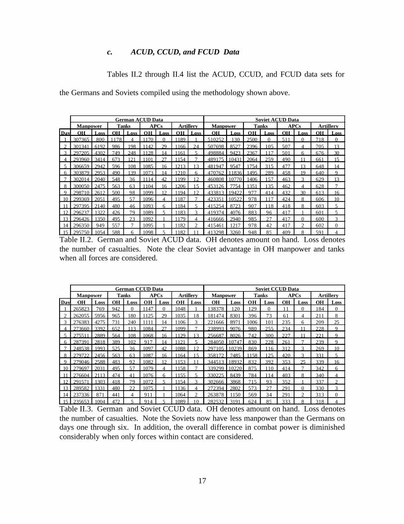
c. ACUD, CCUD, and FCUD Data

Tables II.2 through II.4 list the ACUD, CCUD, and FCUD data sets for

the Germans and Soviets compiled using the methodology shown above.

German ACUD Data Soviet ACUD Data

Day OH Loss OH Loss OH Loss OH Loss OH Loss OH Loss OH Loss OH Loss1 307365 800 1178 4 1170 0 1189 1 510252 130 2500 0 511 0 718 02 301341 6192 986 198 1142 29 1166 24 507698 8527 2396 105 507 4 705 133 297205 4302 749 248 1128 14 1161 5 498884 9423 2367 117 501 6 676 304 293960 3414 673 121 1101 27 1154 7 489175 10431 2064 259 490 11 661 155 306659 2942 596 108 1085 16 1213 13 481947 9547 1754 315 477 13 648 146 303879 2953 490 139 1073 14 1210 6 470762 11836 1495 289 458 19 640 97 302014 2040 548 36 1114 42 1199 12 460808 10770 1406 157 463 3 629 138 300050 2475 563 63 1104 16 1206 15 453126 7754 1351 135 462 4 628 79 298710 2612 500 98 1099 12 1194 12 433813 19422 977 414 432 30 613 1610 299369 2051 495 57 1096 4 1187 7 423351 10522 978 117 424 8 606 1011 297395 2140 480 46 1093 6 1184 5 415254 8723 907 118 418 8 603 512 296237 1322 426 79 1089 5 1183 3 419374 4076 883 96 417 1 601 513 296426 1350 495 23 1092 1 1179 4 416666 2940 985 27 417 0 600 314 296350 949 557 7 1095 1 1182 2 415461 1217 978 42 417 2 602 015 295750 1054 588 6 1098 5 1182 11 413298 3260 948 85 409 8 591 4

Manpower Tanks APCs ArtilleryManpower Tanks APCs Artillery

Table II.2. German and Soviet ACUD data. OH denotes amount on hand. Loss denotes the number of casualties. Note the clear Soviet advantage in OH manpower and tanks when all forces are considered.

German CCUD Data Soviet CCUD Data



Table II.3. German and Soviet CCUD data. OH denotes amount on hand. Loss denotes the number of casualties. Note the Soviets now have less manpower than the Germans on days one through six. In addition, the overall difference in combat power is diminished considerably when only forces within contact are considered.

18

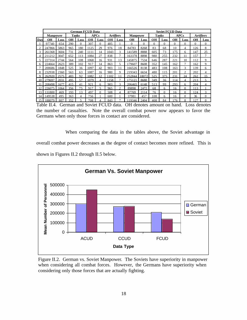
German FCUD Data Soviet FCUD Data



Table II.4. German and Soviet FCUD data. OH denotes amount on hand. Loss denotes the number of casualties. Note the overall combat power now appears to favor the Germans when only those forces in contact are considered.

When comparing the data in the tables above, the Soviet advantage in

overall combat power decreases as the degree of contact becomes more refined. This is

shown in Figures II.2 through II.5 below.

German Vs. Soviet Manpower

0

100000

200000

300000

400000

500000

ACUD CCUD FCUD

Data Type

Mea

n N

umbe

r of

Per

sonn

el

German

Soviet

Figure II.2. German vs. Soviet Manpower. The Soviets have superiority in manpower when considering all combat forces. However, the Germans have superiority when considering only those forces that are actually fighting.

19

German Vs. Soviet Tanks

0

200

400

600

800

1000

1200 1400

1600

ACUD CCUD FCUD

Data Type

Mea

n N

umbe

r of

Tan

ks

German

Soviet

Figure II.3. German vs. Soviet Tanks. The Soviets have more than a two to one advantage in tanks when considering all combat forces. However, the Germans have the advantage when considering only those forces that are actually fighting.

German Vs. Soviet APCs

0

200

400

600

800

1000

1200

ACUD CCUD FCUD

Data Type

Mea

n N

um

ber

of A

PC

s

German

Soviet

Figure II.4. German vs. Soviet APCs. The Germans maintain superiority in the number of APCs in all three data sets.

20

German Vs. Soviet Artillery

0

200

400

600

800

1000

1200

1400

ACUD CCUD FCUD

Data Type

Mea

n N

um

ber

of

Art

iller

y

German

Soviet

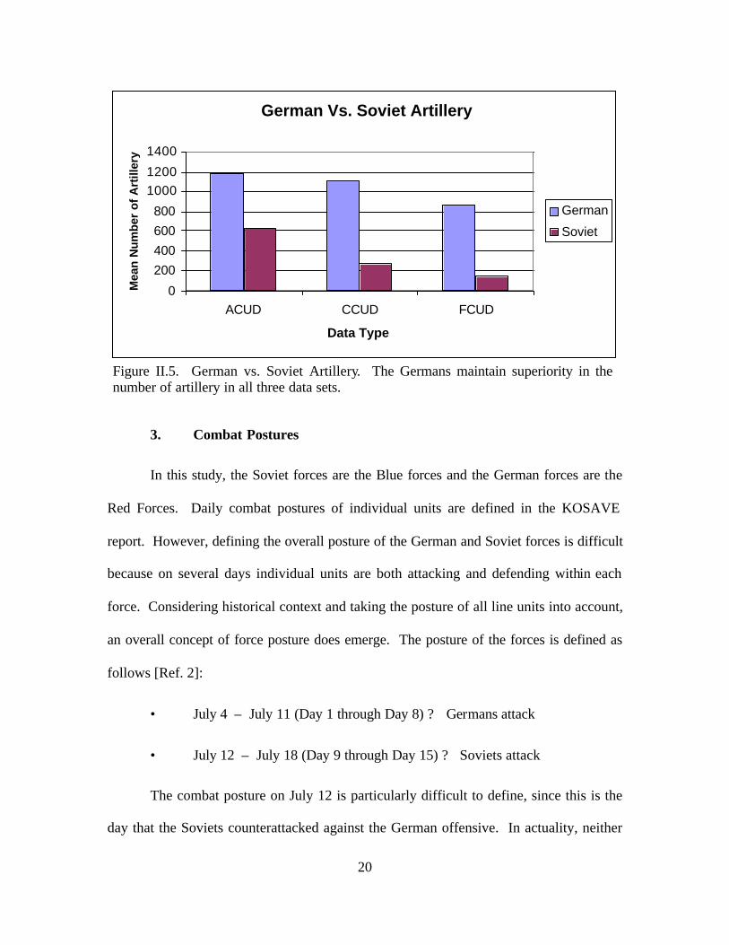
Figure II.5. German vs. Soviet Artillery. The Germans maintain superiority in the number of artillery in all three data sets.

3. Combat Postures

In this study, the Soviet forces are the Blue forces and the German forces are the

Red Forces. Daily combat postures of individual units are defined in the KOSAVE

report. However, defining the overall posture of the German and Soviet forces is difficult

because on several days individual units are both attacking and defending within each

force. Considering historical context and taking the posture of all line units into account,

an overall concept of force posture does emerge. The posture of the forces is defined as

follows [Ref. 2]:

• July 4 – July 11 (Day 1 through Day 8) ? Germans attack

• July 12 – July 18 (Day 9 through Day 15) ? Soviets attack

The combat posture on July 12 is particularly difficult to define, since this is the

day that the Soviets counterattacked against the German offensive. In actuality, neither

21

force was defending during this engagement. However, since the Soviets continued to

press the offensive and the Germans assumed a defensive posture in the days that

followed, the Soviets are considered to be attacking on this day.

4. Correlation Analysis

By examining the degree of correlation in each data set, differences in how the

data interact can be discerned. In particular, the correlations that exist in the ACUD,

CCUD, and FCUD data sets may infer which Lanchester models may apply to each data

set. Figures II.6 through II.8 display simultaneous pair-wise scatter plots of Soviet losses

(SL), German losses (GL), German on-hand (G), and Soviet on-hand (S). [Ref. 11] Each

square within the figure represents a scatterplot of two of the four variables of interest,

shown on the diagonal. A smoothed line is added to better convey the correlation

revealed by the scatterplots. Tables II.5 through II.7 display the correlation matrices that

correspond to the figures. [Ref. 12] Because historical accounts indicate that the battle

did not actually intensify until Day 2, the data for Day 1 are excluded from this analysis.

Each point on the plot corresponds to one of the last 14 days of the data sets. The data

for each day are weighted using Bracken’s approach [Ref. 4] to form a homogeneous

force level of combat losses and combat power (homogeneous on-hand forces) for both

the Soviet and German forces. This weighting process is explained in greater detail in

Chapter III.A.1.a.

For the ACUD data, all interactions are positively correlated. The strongest

correlation of 0.91 occurs between Soviet combat power and German losses. German

combat power and Soviet losses also have a relatively high positive correlation of 0.65.

These results reveal that a force’s casualty levels tend to increase as the enemy’s combat

22

power increases, indicating that a Lanchester square model may be the best fit for the

ACUD data.

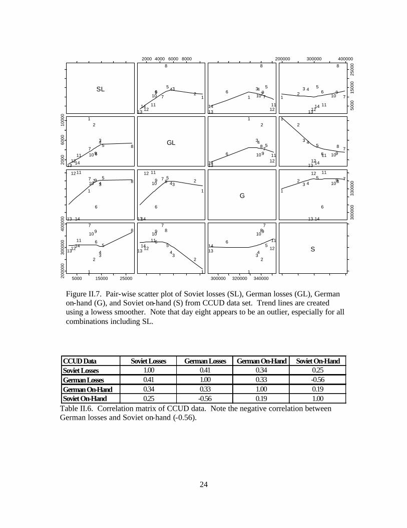
For the CCUD data, a negative correlation of -0.56 exists between German losses

and Soviet combat power, indicating that an increase in Soviet combat power results in a

decrease in German losses. All other correlations exhibit relatively weak positive

correlation. These results suggest that a Lanchester logarithmic model may be the best fit

for the CCUD data.

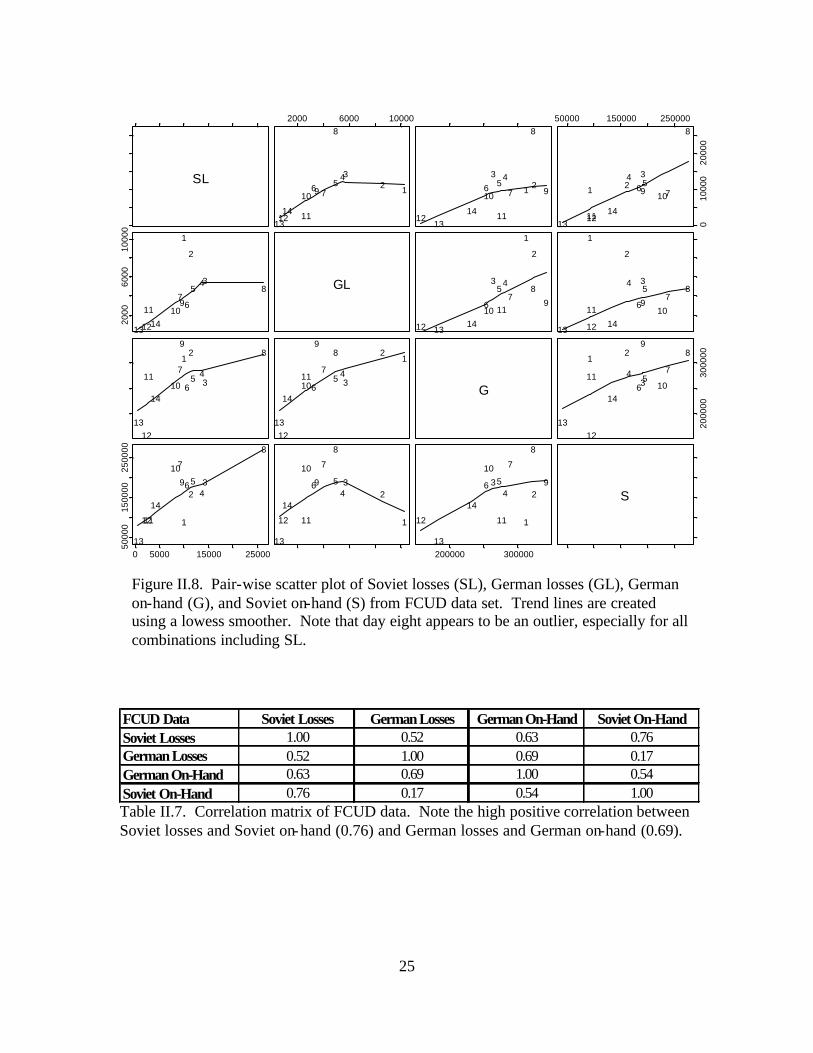
For the FCUD data, all interactions are positively correlated, with German losses

and German combat power (0.69) and Soviet losses and Soviet combat power (0.76)

being the strongest. In addition, the correlation of 0.63 between German losses and

Soviet combat power is also somewhat high. These results indicate that a force’s losses

correspond to both enemy and friendly force strengths, representative of the Lanchester

linear law.

Two additional peculiarities are evident in each figure. Within each data set, the

pair-wise scatterplots indicate that the eighth day of the battle represents an extreme

outlier, especially for all combinations including Soviet losses. This day represents the

large tank battle at Prokhorovka. The exceedingly high casualties that occurred on this

day may exert a high degree of influence on subsequent analysis. In addition, days one

and two also seem to be influential, especially in the CCUD and FCUD analyses. In

particular, the negative correlation in the CCUD analysis and weak positive correlation in

the FCUD analysis, each with respect to German losses and Soviet on-hand, may be

attributed to the influence of days one and two. These are the days in which the Germans

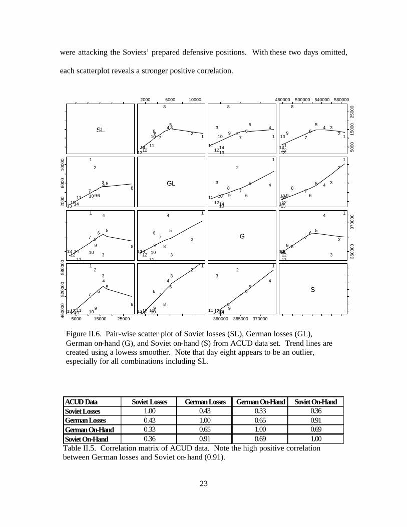
23

were attacking the Soviets’ prepared defensive positions. With these two days omitted,

each scatterplot reveals a stronger positive correlation.

SL

2000 6000 10000

12

345

67

8

910

111213

14

12

3 45

67

8

910

111213

14

460000 500000 540000 580000

5000

1500

025

000

12

345

67

8

910

111213

14

2000

6000

1000

0 1

2

34 5

67

8

9101112

13 14

GL

1

2

3 45

67

8

9101112

1314

1

2

345

67

8

91011121314

1

2

3

4

567

89

10

1112

13 14

1

2

3

4

567

89

10

1112

1314

G

3600

0037

0000

1

2

3

4

567

89

10

11121314

5000 15000 250004600

0052

0000

5800

00 12

34

56

7

89

10111213 14

12

34

56

7

89

1011121314360000 365000 370000

12

34

56

7

89

1011 121314

S

Figure II.6. Pair-wise scatter plot of Soviet losses (SL), German losses (GL), German on-hand (G), and Soviet on-hand (S) from ACUD data set. Trend lines are created using a lowess smoother. Note that day eight appears to be an outlier, especially for all combinations including SL.

ACUD Data Soviet Losses German Losses German On-Hand Soviet On-HandSoviet Losses 1.00 0.43 0.33 0.36German Losses 0.43 1.00 0.65 0.91German On-Hand 0.33 0.65 1.00 0.69Soviet On-Hand 0.36 0.91 0.69 1.00 Table II.5. Correlation matrix of ACUD data. Note the high positive correlation between German losses and Soviet on-hand (0.91).

24

SL

2000 4000 6000 8000

12

3456

7

8

910

111213

14

12

34 56

7

8

910

111213

14

200000 300000 400000

5000

1500

025

000

12

3 4 56

7

8

910

111213

14

2000

6000

1000

0

12

345

67 8

9101112

13 14

GL

12

345

678

910 1112

1314

12

3 45

678

9101112

13 14

1

234

5

6

7 8910

1112

13 14

1

234

5

6

7 8910

1112

1314

G

3000

0033

0000

1

23 4

5

6

78910

1112

13 14

5000 15000 250002000

0030

0000

4000

00

1

234

56

78910

11

121314

1

23

4

56

78910

11

121314

300000 320000 3400001

234

56

78910

11

121314 S

Figure II.7. Pair-wise scatter plot of Soviet losses (SL), German losses (GL), German on-hand (G), and Soviet on-hand (S) from CCUD data set. Trend lines are created using a lowess smoother. Note that day eight appears to be an outlier, especially for all combinations including SL.

CCUD Data Soviet Losses German Losses German On-Hand Soviet On-HandSoviet Losses 1.00 0.41 0.34 0.25German Losses 0.41 1.00 0.33 -0.56German On-Hand 0.34 0.33 1.00 0.19Soviet On-Hand 0.25 -0.56 0.19 1.00

Table II.6. Correlation matrix of CCUD data. Note the negative correlation between German losses and Soviet on-hand (-0.56).

25

SL

2000 6000 10000

1234

56 7

8

910

111213

14

1 23 4

56 7

8

910

111213

14

50000 150000 250000

010

000

2000

0

1 23456 7

8

9 10

111213

14

2000

6000

1000

0

1

2

345

67

8

91011

121314

GL

1

2

3 45

67

8

910 11

12 1314

1

2

345

67

8

91011

121314

12

345

6

7

89

1011

1213

14

12

345

6

7

89

1011

1213

14G

2000

0030

00001

2

34 5

6

7

89

1011

1213

14

0 5000 15000 25000

5000

015

0000

2500

00

1

23

456

7

8

9

10

1112

13

14

1

23

456

7

8

9

10

1112

13

14

200000 300000

1

23

456

7

8

9

10

1112

13

14S

Figure II.8. Pair-wise scatter plot of Soviet losses (SL), German losses (GL), German on-hand (G), and Soviet on-hand (S) from FCUD data set. Trend lines are created using a lowess smoother. Note that day eight appears to be an outlier, especially for all combinations including SL.

FCUD Data Soviet Losses German Losses German On-Hand Soviet On-HandSoviet Losses 1.00 0.52 0.63 0.76German Losses 0.52 1.00 0.69 0.17German On-Hand 0.63 0.69 1.00 0.54Soviet On-Hand 0.76 0.17 0.54 1.00 Table II.7. Correlation matrix of FCUD data. Note the high positive correlation between Soviet losses and Soviet on-hand (0.76) and German losses and German on-hand (0.69).

26


27

III. EXPLORATION OF DATA SETS AND WEIGHTING METHODOLOGIES

A. COMPARATIVE ANALYSIS OF PREVIOUS METHODOLOGIES

In this section, the methodologies previously implemented by Bracken and Turkes

are applied to the ACUD, CCUD, and FCUD data sets. First, a summary of the original

methodologies is given in each subsection. The analysis is then completed with strict

adherence to the respective methodology, and the results are compared to Turkes’ results

from his analysis of the Battle of Kursk. The objective of this analysis is to analyze the

impact of using only engaged and partially engaged forces to determine Lanchester

parameters.

1. Bracken Methodology

a. Summary

Bracken’s study [Ref. 4] involved the parameter estimation for Lanchester

equations when applied to the Ardennes campaign of World War II. He was also

interested in the tactical posture of a force and its effect on attrition. Bracken used the

following variation of the basic Lanchester equations to perform his analysis:

B& (t) = adR(t)pB(t)q, (III.1)

R& (t) = b(1/d)B(t)pR(t)q (III.2)

The a, b, p, and q parameters in these equations have the same definition

as those presented in Chapter I.B.1. The d parameter is a tactical parameter that Bracken

introduced to determine whether the attacker or defender had any advantage in the battle.

28

The use of d in Equations III.1 and III.2 implies that Red is attacking and Blue is

defending. Interpretation of d is as follows:

d > 1 ? attacker advantage exists

d = 1 ? neither attacker nor defender advantage exists

d < 1 ? defender advantage exists

Bracken divides his analysis into four separate models. Each model

requires an aggregation of manpower, APCs, tanks, and artillery into a homogeneous

representation of combat power. This is accomplished by multiplying the actual size of

each force type by an appropriate weighting parameter and summing for each day:

(III.3)

Bracken used the following weighting parameters in his analysis: 1 for

personnel, 20 for tanks, 5 for APCs, and 40 for artillery. He assumed these weights based

on weighting methods he claimed were used by CAA. He further states [Ref. 4] that,

“Virtually all theater- level dynamic combat simulation models incorporate similar

weights, either as inputs or as decision parameters computed as the simulations progress.”

In Model 1, force strengths are represented by tanks, APCs, artillery, and

combat manpower. Bracken defines combat manpower as infantry, armor, and artillery

personnel only. In Model 2, combat manpower is substituted with total manpower;

which is defined as all personnel in the campaign, including logistics and support

( )( )

( ) 4 to1 for ,40 5, 20, 1,

4 to1 for ,Artillery of # APCs, of # Tanks, of # Personnel, of #

campaign theof days theindexes 15.........1

,4

1

==

==

=

∀×∑==

ii

Weight

iiType

n

ni

Weighti

TyperCombatPowei

29

personnel. Models 3 and 4 consist of the same forces as Models 1 and 2, respectively,

but exclude the use of a tactical parameter.

Bracken’s methodology involved defining a discrete set of values for each

of the parameters in the model (i.e. a, b, d, p, q). He then performed a search over this

grid of parameter values for the set of parameters resulting in the lowest sum of squared

residuals when compared to the actual data. The sum of squared residuals was calculated

using the Equation III.4 below:

(III.4)

where n represents the days of the battle, B& n and R& n are the actual number of Soviet and

German casualties on day n, and B n and R n are the actual number on-hand. In this

model, the Germans attacked on days two through six and the Allies attacked on days

seven through eleven. Bracken eliminated day one from consideration since no

significant contact occurred on this day.

The results of Bracken’s analysis are shown in Table III.1.

Model Type a b p q d

Model 1 8.00E-09 1.00E-08 1 1 1.25

Model 2 8.00E-09 8.00E-09 0.8 1.2 1.25

Model 3 8.00E-09 1.00E-08 1.3 0.7 N/A

Model 4 8.00E-09 8.00E-09 1.2 0.8 N/A Table III.1. Resulting parameters of Bracken’s analysis of the Ardennes campaign data.

( ) ( )( ) ( )

211

7

211

7

26

2

26

2

)/1(

)/1(

∑∑

∑∑

==

==

−−+

−−=

+

+

nn

nn

qn

pnn

qn

pnn

qn

pnn

qn

pnn

RbdBRBRdaB

RBdbRBadRBSSR

&&

&&

30

Bracken concluded the following from his analysis:

• The Lanchester linear model results in the best fit for the Ardennes campaign in all four models.

• When considering combat forces, Allied individual effectiveness is greater than German individual effectiveness.

• When considering total forces, individual effectiveness is the same for both sides.

• An attacker advantage exists throughout the campaign.

b. Aggregation of Data

The following analysis directly applies Bracken’s weighting methodology

to the three data sets from the Battle of Kursk defined in Chapter II.B.2.c. Tables III.2

and III.3 present the aggregated data for all three data sets.

German On-Hand German Casualt iesD a y A C U D C C U D F C U D A C U D C C U D F C U D

1 384335 332318 121275 920 809 6942 373411 328380 311831 11257 10421 103283 364265 340798 323263 9532 9265 85944 359085 336080 263192 6249 6067 57225 372524 337291 281174 5702 5649 55046 367444 344596 271549 6043 5128 49337 366504 308043 252791 3450 3403 32188 365070 342977 288833 4415 4396 40609 361965 340236 322070 5112 4928 4915

10 362229 341312 341312 3491 3471 347111 359820 337664 257523 3290 3163 264712 357522 351451 276380 3047 3028 266913 358946 349997 158465 1975 1936 88914 360245 293271 184578 1174 1036 62015 360280 293223 232379 1639 1529 1207

Table III.2. Aggregated data for German forces. Aggregated force data is obtained by weighting combat manpower, tanks, APCs, and artillery by 1, 20, 5, and 40, respectively.

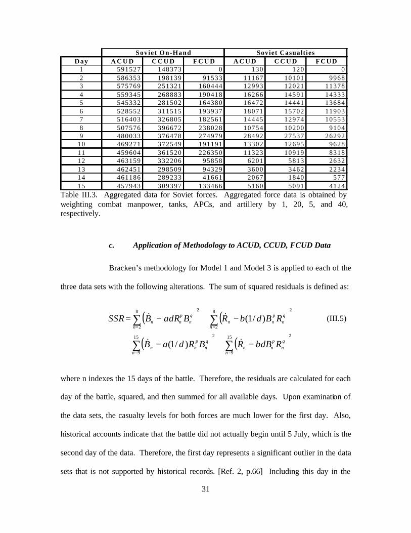
31

Soviet On-Hand Soviet CasualtiesD a y A C U D C C U D F C U D A C U D C C U D F C U D

1 591527 148373 0 130 120 02 586353 198139 91533 11167 10101 99683 575769 251321 160444 12993 12021 113784 559345 268883 190418 16266 14591 143335 545332 281502 164380 16472 14441 136846 528552 311515 193937 18071 15702 119037 516403 326805 182561 14445 12974 105538 507576 396672 238028 10754 10200 91049 480033 376478 274979 28492 27537 26292

10 469271 372549 191191 13302 12695 962811 459604 361520 226350 11323 10919 831812 463159 332206 95858 6201 5813 263213 462451 298509 94329 3600 3462 223414 461186 289233 41661 2067 1840 57715 457943 309397 133466 5160 5091 4124

Table III.3. Aggregated data for Soviet forces. Aggregated force data is obtained by weighting combat manpower, tanks, APCs, and artillery by 1, 20, 5, and 40, respectively.

c. Application of Methodology to ACUD, CCUD, FCUD Data

Bracken’s methodology for Model 1 and Model 3 is applied to each of the

three data sets with the following alterations. The sum of squared residuals is defined as:

(III.5)

where n indexes the 15 days of the battle. Therefore, the residuals are calculated for each

day of the battle, squared, and then summed for all available days. Upon examination of

the data sets, the casualty levels for both forces are much lower for the first day. Also,

historical accounts indicate that the battle did not actually begin until 5 July, which is the

second day of the data. Therefore, the first day represents a significant outlier in the data

sets that is not supported by historical records. [Ref. 2, p.66] Including this day in the

( ) ( )

( ) ( )215

9

215

9

28

2

28

2

)/1(

)/1(

∑∑

∑∑

==

==

−+−+

−+−=

n

qn

pnn

n

qn

pnn

n

qn

pnn

n

qn

pnn

RbdBRBRdaB

RBdbRBadRBSSR

&&

&&

32

analysis could have adverse effects on the results. Thus, only the last 14 days of the data

set are used in the remainder of this thesis. Other possible outliers in the data sets that

occur during the course of the battle are included. This analysis portrays the Germans on

the offensive on days two through eight and the Soviets on the offensive on days nine

through 15. The parameters a, d, p, and q are limited to the following discrete range:

(a1,............,a9) = (4 x 10-9,............,1.2x10-8),

(b1,............,b9) = (4 x 10-9,............,1.2x10-8),

(p1,............,p21) = (0.0,............,2.0),

(q1,............,q21) = (0.0,............,2.0),

(d1,............,d9) = (0.6,............,1.4).

This is the range of parameters used by Turkes [Ref. 2] in his application

of Bracken’s methodology. It includes a more comprehensive set of parameters than

those used by Bracken.

d. Results

Tables III.4 and III.5 illustrate the results of Bracken’s search method

when applied to the ACUD, CCUD, and FCUD data sets for Models 1 and 3.

Data Set a b p q d SSR R2

ACUD 1.20E-08 1.00E-08 0.1 2.0 1.0 6.51E+08 0.0919

CCUD 9.00E-09 4.00E-09 0.9 1.3 1.1 6.26E+08 0.0019

FCUD 1.20E-08 8.00E-09 1.7 0.5 1.0 3.99E+08 0.3809

Table III.4. Results of Bracken's method when applied to Model 1. ACUD results most resemble the logarithmic law, CCUD results most resemble a mix of the logarithmic and linear laws, and FCUD results most resemble the square law.

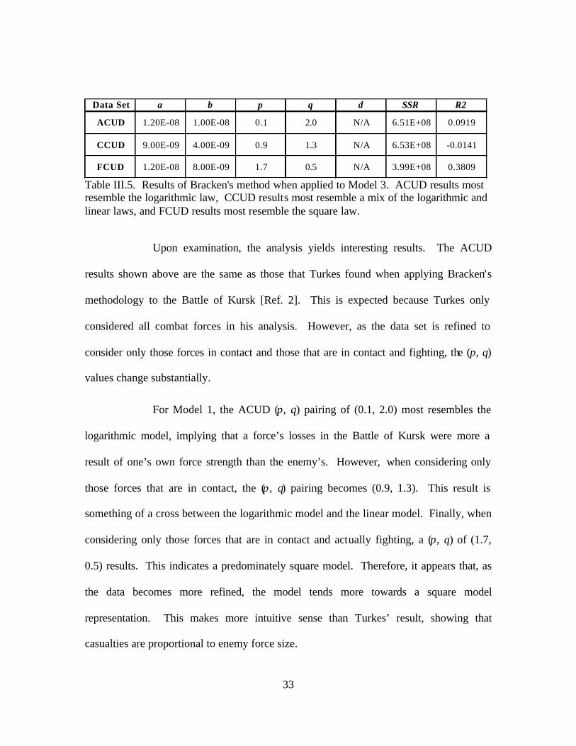
33

Data Set a b p q d SSR R2

ACUD 1.20E-08 1.00E-08 0.1 2.0 N/A 6.51E+08 0.0919

CCUD 9.00E-09 4.00E-09 0.9 1.3 N/A 6.53E+08 -0.0141

FCUD 1.20E-08 8.00E-09 1.7 0.5 N/A 3.99E+08 0.3809

Table III.5. Results of Bracken's method when applied to Model 3. ACUD results most resemble the logarithmic law, CCUD results most resemble a mix of the logarithmic and linear laws, and FCUD results most resemble the square law.

Upon examination, the analysis yields interesting results. The ACUD

results shown above are the same as those that Turkes found when applying Bracken’s

methodology to the Battle of Kursk [Ref. 2]. This is expected because Turkes only

considered all combat forces in his analysis. However, as the data set is refined to

consider only those forces in contact and those that are in contact and fighting, the (p, q)

values change substantially.

For Model 1, the ACUD (p, q) pairing of (0.1, 2.0) most resembles the

logarithmic model, implying that a force’s losses in the Battle of Kursk were more a

result of one’s own force strength than the enemy’s. However, when considering only

those forces that are in contact, the (p, q) pairing becomes (0.9, 1.3). This result is

something of a cross between the logarithmic model and the linear model. Finally, when

considering only those forces that are in contact and actually fighting, a (p, q) of (1.7,

0.5) results. This indicates a predominately square model. Therefore, it appears that, as

the data becomes more refined, the model tends more towards a square model

representation. This makes more intuitive sense than Turkes’ result, showing that

casualties are proportional to enemy force size.

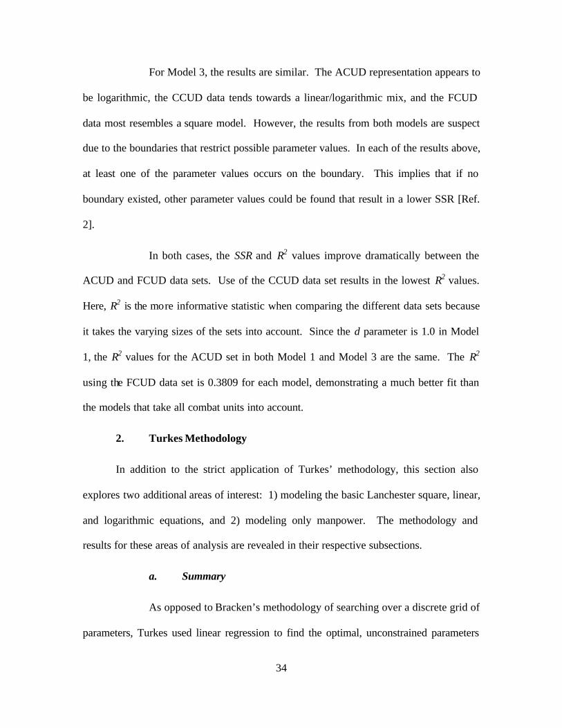
34

For Model 3, the results are similar. The ACUD representation appears to

be logarithmic, the CCUD data tends towards a linear/logarithmic mix, and the FCUD

data most resembles a square model. However, the results from both models are suspect

due to the boundaries that restrict possible parameter values. In each of the results above,

at least one of the parameter values occurs on the boundary. This implies that if no

boundary existed, other parameter values could be found that result in a lower SSR [Ref.

2].

In both cases, the SSR and R2 values improve dramatically between the

ACUD and FCUD data sets. Use of the CCUD data set results in the lowest R2 values.

Here, R2 is the more informative statistic when comparing the different data sets because

it takes the varying sizes of the sets into account. Since the d parameter is 1.0 in Model

1, the R2 values for the ACUD set in both Model 1 and Model 3 are the same. The R2

using the FCUD data set is 0.3809 for each model, demonstrating a much better fit than

the models that take all combat units into account.

2. Turkes Methodology

In addition to the strict application of Turkes’ methodology, this section also

explores two additional areas of interest: 1) modeling the basic Lanchester square, linear,

and logarithmic equations, and 2) modeling only manpower. The methodology and

results for these areas of analysis are revealed in their respective subsections.

a. Summary

As opposed to Bracken’s methodology of searching over a discrete grid of

parameters, Turkes used linear regression to find the optimal, unconstrained parameters

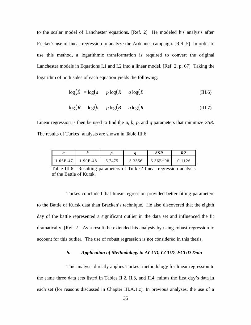
35

to the scalar model of Lanchester equations. [Ref. 2] He modeled his analysis after

Fricker’s use of linear regression to analyze the Ardennes campaign. [Ref. 5] In order to

use this method, a logarithmic transformation is required to convert the original

Lanchester models in Equations I.1 and I.2 into a linear model. [Ref. 2, p. 67] Taking the

logarithm of both sides of each equation yields the following:

( ) ( ) ( ) ( )BqRpaB loglogloglog ++=& (III.6)

( ) ( ) ( ) ( )RqBpbR loglogloglog ++=& (III.7)

Linear regression is then be used to find the a, b, p, and q parameters that minimize SSR.

The results of Turkes’ analysis are shown in Table III.6.

a b p q SSR R2

1.06E-47 1.90E-48 5.7475 3.3356 6.36E+08 0.1126

Table III.6. Resulting parameters of Turkes’ linear regression analysis of the Battle of Kursk.

Turkes concluded that linear regression provided better fitting parameters

to the Battle of Kursk data than Bracken’s technique. He also discovered that the eighth

day of the battle represented a significant outlier in the data set and influenced the fit

dramatically. [Ref. 2] As a result, he extended his analysis by using robust regression to

account for this outlier. The use of robust regression is not considered in this thesis.

b. Application of Methodology to ACUD, CCUD, FCUD Data

This analysis directly applies Turkes’ methodology for linear regression to

the same three data sets listed in Tables II.2, II.3, and II.4, minus the first day’s data in

each set (for reasons discussed in Chapter III.A.1.c). In previous analyses, the use of a

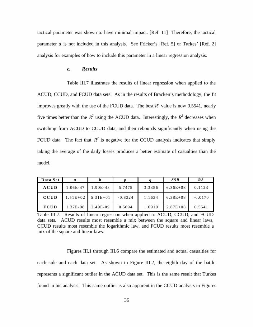
36

tactical parameter was shown to have minimal impact. [Ref. 11] Therefore, the tactical

parameter d is not included in this analysis. See Fricker’s [Ref. 5] or Turkes’ [Ref. 2]

analysis for examples of how to include this parameter in a linear regression analysis.

c. Results

Table III.7 illustrates the results of linear regression when applied to the

ACUD, CCUD, and FCUD data sets. As in the results of Bracken’s methodology, the fit

improves greatly with the use of the FCUD data. The best R2 value is now 0.5541, nearly

five times better than the R2 using the ACUD data. Interestingly, the R2 decreases when

switching from ACUD to CCUD data, and then rebounds significantly when using the

FCUD data. The fact that R2 is negative for the CCUD analysis indicates that simply

taking the average of the daily losses produces a better estimate of casualties than the

model.

Data Set a b p q SSR R2

A C U D 1.06E-47 1.90E-48 5.7475 3 .3356 6.36E+08 0.1123

C C U D 1.51E+02 5.31E+01 -0.8324 1 .1634 6.38E+08 -0.0170

F C U D 1.37E-08 2.49E-09 0.5694 1 .6919 2.87E+08 0.5541

Table III.7. Results of linear regression when applied to ACUD, CCUD, and FCUD data sets. ACUD results most resemble a mix between the square and linear laws, CCUD results most resemble the logarithmic law, and FCUD results most resemble a mix of the square and linear laws.

Figures III.1 through III.6 compare the estimated and actual casualties for

each side and each data set. As shown in Figure III.2, the eighth day of the battle

represents a significant outlier in the ACUD data set. This is the same result that Turkes

found in his analysis. This same outlier is also apparent in the CCUD analysis in Figures

37

III.3 and III.4, while the fit for the German losses appears to be worse than the ACUD fit.

In addition, the CCUD model overestimates casualties for both sides from Day 11

through Day 14. The combination of these effects may explain why the R2 is lower for

the CCUD analysis than the ACUD analysis. However, as shown in Figures III.5 and

III.6, the fits improve dramatically when using the FCUD data, especially for the Soviet

forces. In fact, Figure III.6 reveals that the model now accounts for the data point that

was an outlier in the ACUD and CCUD analyses. The only identifiable weakness in the

FCUD model occurs in the first few days of the battle, where the model underestimates

the real German casualties. Since these days correspond to Germany’s initial assault on

prepared defensive positions, this result is somewhat expected. The estimated parameters

reflect the entire course of the campaign. Therefore, a relatively short period of intense

combat may result in a higher residual value for that time period.

The parameters found for the ACUD data most resemble a cross between

the square and linear models, with a unit’s casualties tending to be more proportional to

the enemy’s force size. The CCUD parameters most resemble the logarithmic model,

indicating that a unit’s casualties are a function of its own force size. However, the fact

that the p parameter is negative is counterintuitive, indicating that an increase in enemy

force size actually benefits the friendly force. The FCUD results indicate a mixture of the

linear and logarithmic models, with a unit’s casualties tending to be more proportional to

its own force size. These results coincide with the expected Lanchester models from the

correlation analysis in Chapter II.B.4.

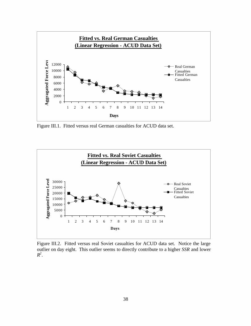
38

Fitted vs. Real German Casualties (Linear Regression - ACUD Data Set)

0

2000

4000

6000

8000

10000

12000

1 2 3 4 5 6 7 8 9 10 11 12 13 14

Days

Agg

raga

ted

For

ce L

evel

Real GermanCasualtiesFitted GermanCasualties

Figure III.1. Fitted versus real German casualties for ACUD data set.

Fitted vs. Real Soviet Casualties (Linear Regression - ACUD Data Set)

0

500010000

1500020000

2500030000

1 2 3 4 5 6 7 8 9 10 11 12 13 14

Days

Agg

raga

ted

Forc

e L

evel

Real SovietCasualtiesFitted SovietCasualties

Figure III.2. Fitted versus real Soviet casualties for ACUD data set. Notice the large outlier on day eight. This outlier seems to directly contribute to a higher SSR and lower R2.

39

Fitted vs. Real German Casualties (Linear Regression - CCUD Data Set)

0

20004000

6000

800010000

12000

1 2 3 4 5 6 7 8 9 10 11 12 13 14

Days

Agg

raga

ted

Forc

e L

evel


Figure III.3. Fitted versus real German casualties for CCUD data set. Notice the fit appears to be much worse than the fit in Figure III.1.

Fitted vs. Real Soviet Casualties (Linear Regression - CCUD Data Set)

05000

100001500020000

2500030000

1 2 3 4 5 6 7 8 9 10 11 12 13 14

Days

Agg

raga

ted

Forc

e L

evel


Figure III.4. Fitted versus real Soviet casualties for CCUD data set. Notice the large outlier on day eight. This outlier seems to directly contribute to a higher SSR and lower R2.

40

Fitted vs. Real German Casualties (Linear Regression - FCUD Data Set)

0

2000

4000

6000

8000

10000

12000

1 2 3 4 5 6 7 8 9 10 11 12 13 14

Days

Agg

raga

ted

For

ce L

evel


Figure III.5. Fitted versus real German casualties for FCUD data set. Except for the first two days, the fit appears much better than the CCUD analysis.

Fitted vs. Real Soviet Casualties (Linear Regression - FCUD Data Set)

05000

100001500020000250003000035000

1 2 3 4 5 6 7 8 9 10 11 12 13 14

Days

Agg

raga

ted

For

ce L

evel


Figure III.6. Fitted versus real Soviet casualties for FCUD data set. Notice how the model’s fitted casualties now closely resemble the real casualties. Most significantly, the model more accurately estimates the casualties from day eight. This greatly decreases the SSR and increases R2.

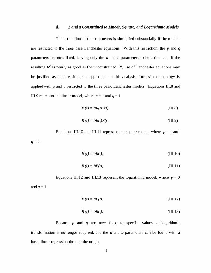
41

d. p and q Constrained to Linear, Square, and Logarithmic Models

The estimation of the parameters is simplified substantially if the models

are restricted to the three base Lanchester equations. With this restriction, the p and q

parameters are now fixed, leaving only the a and b parameters to be estimated. If the

resulting R2 is nearly as good as the unconstrained R2, use of Lanchester equations may

be justified as a more simplistic approach. In this analysis, Turkes’ methodology is

applied with p and q restricted to the three basic Lanchester models. Equations III.8 and

III.9 represent the linear model, where p = 1 and q = 1.

B& (t) = aR(t)B(t), (III.8)

R& (t) = bB(t)R(t), (III.9)

Equations III.10 and III.11 represent the square model, where p = 1 and

q = 0.

B& (t) = aR(t), (III.10)

R& (t) = bB(t), (III.11)

Equations III.12 and III.13 represent the logarithmic model, where p = 0

and q = 1.

B& (t) = aB(t), (III.12)

R& (t) = bR(t), (III.13)

Because p and q are now fixed to specific values, a logarithmic

transformation is no longer required, and the a and b parameters can be found with a

basic linear regression through the origin.

42

The results of this analysis are shown in Tables III.8 through III.10. Of

the basic Lanchester laws, the linear law provides the best fit for the ACUD data, the

logarithmic law provides the best fit for the CCUD data, and the linear law provides the

best fit for the FCUD data. Overall, the linear model with FCUD data provides the best

fit. With an R2 value of 0.5513, the performance of the model is very close to the

performance of the FCUD model found with unconstrained values for p and q. This

indicates that the Lanchester linear model provides an excellent fit for the FCUD data.

The scale of the a and b parameters is also of interest here. The results of

the unrestricted analysis in Table III.7 show widely varying results for the a and b

parameters. However, as explained earlier, when the p and q values are restricted, a

logarithmic transformation of the data is no longer required. Therefore, the use of basic

linear regression to estimate a and b appears to result in more consistent values across the

models. In addition, the fact that the p and q parameters are fixed to the same values for

each data set also contributes to the consistency of the a and b parameters.

Model a b p q SSR R2

Linear 2.17E-07 8.26E-08 1 1 5.03E+08 0.5513

Square 3.72E-02 2.34E-02 1 0 2.89E+08 0.2185

Log 6.13E-02 1.63E-02 0 1 3.08E+08 0.5216

Table III.8. Linear regression results for FCUD data with p and q restricted to Lanchester linear, square, and logarithmic models. Note the high R2 value for the linear model.

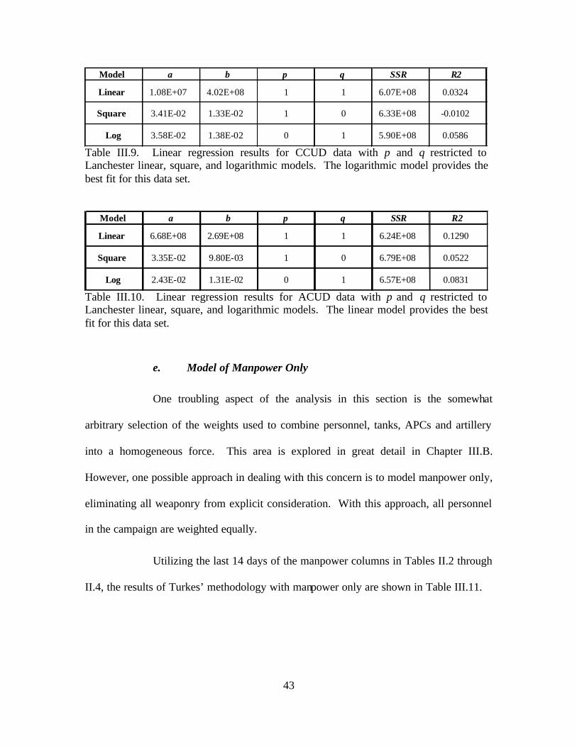
43


Linear 1.08E+07 4.02E+08 1 1 6.07E+08 0.0324

Square 3.41E-02 1.33E-02 1 0 6.33E+08 -0.0102

Log 3.58E-02 1.38E-02 0 1 5.90E+08 0.0586

Table III.9. Linear regression results for CCUD data with p and q restricted to Lanchester linear, square, and logarithmic models. The logarithmic model provides the best fit for this data set.


Linear 6.68E+08 2.69E+08 1 1 6.24E+08 0.1290

Square 3.35E-02 9.80E-03 1 0 6.79E+08 0.0522

Log 2.43E-02 1.31E-02 0 1 6.57E+08 0.0831

Table III.10. Linear regression results for ACUD data with p and q restricted to Lanchester linear, square, and logarithmic models. The linear model provides the best fit for this data set.

e. Model of Manpower Only

One troubling aspect of the analysis in this section is the somewhat

arbitrary selection of the weights used to combine personnel, tanks, APCs and artillery

into a homogeneous force. This area is explored in great detail in Chapter III.B.

However, one possible approach in dealing with this concern is to model manpower only,

eliminating all weaponry from explicit consideration. With this approach, all personnel

in the campaign are weighted equally.

Utilizing the last 14 days of the manpower columns in Tables II.2 through

II.4, the results of Turkes’ methodology with manpower only are shown in Table III.11.

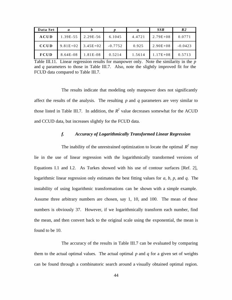
44

Data Set a b p q SSR R2

A C U D 1.39E-55 2.29E-56 6.1045 4 .4721 2.79E+08 0.0771

C C U D 9.81E+02 3.45E+02 -0.7752 0.925 2.90E+08 -0.0423

F C U D 8.64E-08 1.81E-08 0.5214 1 .5614 1.17E+08 0.5713

Table III.11. Linear regression results for manpower only. Note the similarity in the p and q parameters to those in Table III.7. Also, note the slightly improved fit for the FCUD data compared to Table III.7.

The results indicate that modeling only manpower does not significantly

affect the results of the analysis. The resulting p and q parameters are very similar to

those listed in Table III.7. In addition, the R2 value decreases somewhat for the ACUD

and CCUD data, but increases slightly for the FCUD data.

f. Accuracy of Logarithmically Transformed Linear Regression

The inability of the unrestrained optimization to locate the optimal R2 may

lie in the use of linear regression with the logarithmically transformed versions of

Equations I.1 and I.2. As Turkes showed with his use of contour surfaces [Ref. 2],

logarithmic linear regression only estimates the best fitting values for a, b, p, and q. The

instability of using logarithmic transformations can be shown with a simple example.

Assume three arbitrary numbers are chosen, say 1, 10, and 100. The mean of these

numbers is obviously 37. However, if we logarithmically transform each number, find

the mean, and then convert back to the original scale using the exponential, the mean is

found to be 10.

The accuracy of the results in Table III.7 can be evaluated by comparing

them to the actual optimal values. The actual optimal p and q for a given set of weights

can be found through a combinatoric search around a visually obtained optimal region.

45

[Ref. 11] The p and q parameters are assigned discrete values over a specified range and

a R2 value is calculated for each combination. The a and b parameters for each

combination are calculated by a straightforward linear regression through the origin. The

p and q values that result in the highest R2 are optimal. The results of this search are

shown in Table III.12.

D a t a S e t a b p q SSR R 2

A C U D 1 . 8 1 E - 3 5 1 . 4 7 E - 3 6 5 .70 1 .25 5 . 4 7 E + 0 8 0 . 2 3 7 1

C C U D 3 . 0 5 E + 0 0 1 . 1 7 E + 0 0 -0 .35 1 .00 5 . 8 9 E + 0 8 0 . 0 6 0 7

F C U D 3 . 0 7 E - 0 6 8 . 5 1 E - 0 7 0 .40 1 .40 2 . 7 3 E + 0 8 0 . 5 7 6 8

Table III.12. Results of combinatoric search over p and q using Bracken’s weighting criteria. Note the difference in the value of q for the ACUD data as compared to Table III.7.

The contour surfaces of the ACUD, CCUD, and FCUD data sets using

Bracken’s weighting criteria are shown in Figures III.7 through III.9. These surfaces

graphically portray the R2 values for a different combination of p and q and were created

using the method described above by incrementing p and q in steps of 0.05. [Ref. 11]

Each line represents an individual R2 value in increments of 0.02, and the compilation of

all of these lines creates a visual picture of the R2 surface. Based on these surfaces and

the results in Table III.8, the use of linear regression on the logarithmically transformed

equations has mixed results. The actual optimal p value for the ACUD data is 5.70,

which is the nearly the same as the value found through linear regression. However, the

actual q value is 1.25, which differs greatly from the value of 3.3356 found through linear

regression. Because of this, the optimal R2 value found through linear regression on the

logarithmically transformed equations is much less than the actual optimal R2 of 0.2371.

46

However, the results for the CCUD and FCUD data are much better. For

the CCUD data, the optimal p and q values are -0.35 and 1.00, which compare favorably

to the p and q values found through linear regression on the logarithmically transformed

equations. For the FCUD data, the optimal p and q values are 0.40 and 1.40, which are

also close to the linear regression values.

p

q

4 5 6 7

0

1

2

3

4 0.02 0.04 0.06 0.08 0.1 0.12 0.14

0.16

0.16

0.18

0.18

0.2

0.2

0.22

Contour Plot of R -Squared Surface (ACUD Data Set)

p 4 5 6 7

0

1

2

3

4

X - Actual Optimal R -Squared

X - Turkes Optimal R -Squared

Figure III.7. Contour plot of R2 surface for ACUD data set with Bracken’s weights. Note the disparity between the optimal and estimated p and q values.

47

p

q

-2 -1 0 1 2

-1

0

1

2

3

-0.3 -0.25

-0.25

-0.2

-0.2

-0.15

-0.15

-0.1

-0.1

-0.05

-0.05

-0.05

0 0.05

Contour Plot of R -Squared Sur face (CCUD Da ta Set)

p -2 -1 0 1 2

-1

0

1

2

3

X - Actual Optimal R-Squared X - Turkes Opt imal R -Squared

Figure III.8. Contour plot of R2 surface for CCUD data set with Bracken weights. Note the close proximity between the optimal and estimated p and q values.

p

q

-1 0 1 2 3

0

1

2

3

4

-0.6 -0.5 -0.4 -0.3

-0.2

-0.2

-0.1

-0.1

0

0

0.1

0.1

0.2

0.2

0.2

0.2

0.3

0.3

0.4 0.5

Contour Plot of R -Squared Surface (FCUD Data Set )

p -1 0 1 2 3

0

1

2

3

4

X - Actual Optimal R -Squared X - Turkes Optimal R -Squared

Figure III.9. Contour plot of R2 surface for FCUD data set with Bracken weights. Note the close proximity between the optimal and estimated p and q values.

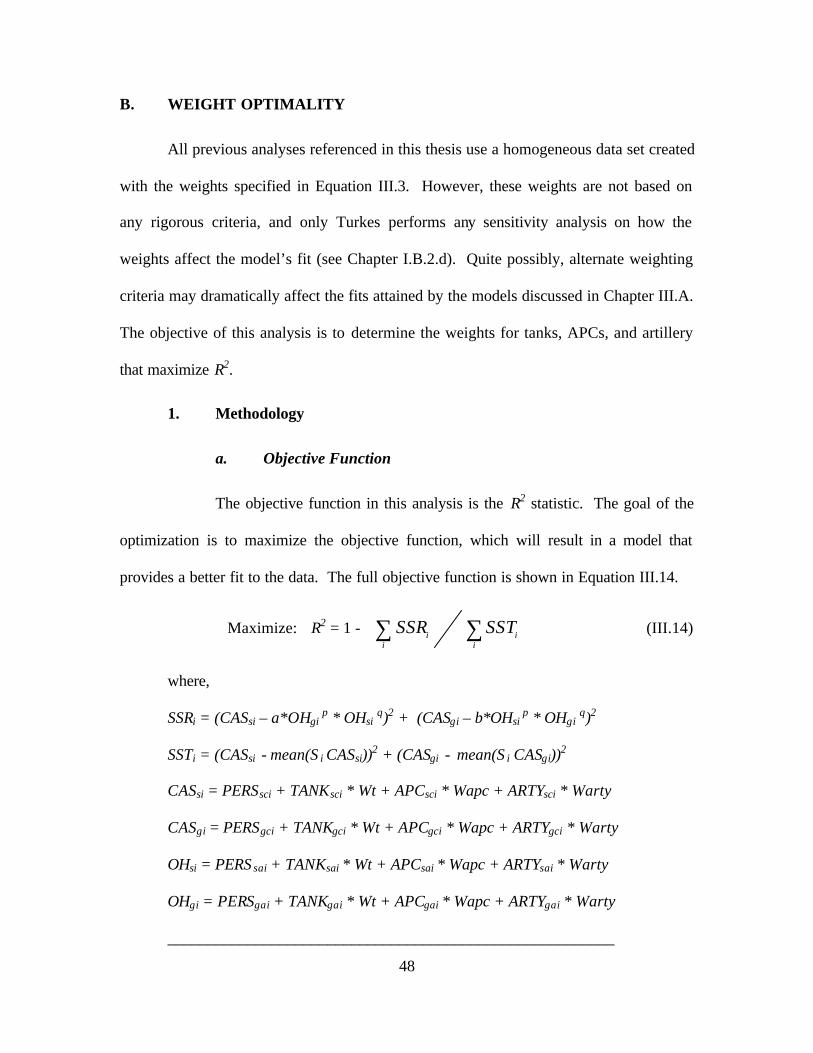
48

B. WEIGHT OPTIMALITY

All previous analyses referenced in this thesis use a homogeneous data set created

with the weights specified in Equation III.3. However, these weights are not based on

any rigorous criteria, and only Turkes performs any sensitivity analysis on how the

weights affect the model’s fit (see Chapter I.B.2.d). Quite possibly, alternate weighting

criteria may dramatically affect the fits attained by the models discussed in Chapter III.A.

The objective of this analysis is to determine the weights for tanks, APCs, and artillery

that maximize R2.

1. Methodology

a. Objective Function

The objective function in this analysis is the R2 statistic. The goal of the

optimization is to maximize the objective function, which will result in a model that

provides a better fit to the data. The full objective function is shown in Equation III.14.

Maximize: R2 = 1 -

∑∑

ii

ii SSTSSR (III.14)

where, SSRi = (CASsi – a*OHgi

p * OHsi q)2 + (CASgi – b*OHsi p * OHgi q)2

SSTi = (CASsi - mean(S i CASsi))2 + (CASgi - mean(S i CASgi))2

CASsi = PERSsci + TANKsci * Wt + APCsci * Wapc + ARTYsci * Warty

CASgi = PERSgci + TANKgci * Wt + APCgci * Wapc + ARTYgci * Warty

OHsi = PERS sai + TANKsai * Wt + APCsai * Wapc + ARTYsai * Warty

OHgi = PERSgai + TANKgai * Wt + APCgai * Wapc + ARTYgai * Warty

________________________________________________________

49

SSRi = sum of squared residuals for day i SSTi = total sum of squares for day i CASxi = # of casualties for force x on day i OHxi = # oh-hand for force x on day i PERSxyi = # of personnel of force type x and status y on day i TANKxyi = # of tanks of force type x and status y on day i APCxyi = # of APCs of force type x and status y on day i ARTYxyi = # of artillery of force type x and status y on day i Wt = tank weight Wapc = APC weight Warty = artillery weight x = (s Soviet, g German) y = (c casualties, a available forces) a = Soviet attrition coefficient b = German attrition coefficient p = exponent parameter of opposing force q = exponent parameter of friendly force i = index of day of battle (1, 2, ..., 14)

As a baseline, personnel weights are assumed to be one in this analysis.

Therefore, the resulting tank, APC, and artillery weights are relative to personnel

weights. Separate analyses are conducted for each of the three data sets. In addition,

analysis of the FCUD data set is conducted with the p and q parameters set to each of the

three standard Lanchester models.

b. Theoretical Summary

The following analysis employs a steepest ascent algorithm in order to

determine the optimal weights. If R2 is represented by f(x), where x = (tank weight, APC

weight, artillery weight), and if f(x) is differentiable at x with a non-zero gradient, then

the gradient of f(x) is the direction of steepest ascent. [Ref. 8: p. 300] Therefore, if d

equals the gradient of f(x) and ? equals the step length, then x can be incremented using

Equation III.15 shown below.

50

x = x + ?d (III.15)

Due to the complexity of the objective function, the gradient of f(x) is

estimated numerically. This is accomplished by incrementing each weight by a certain

distance (?), calculating the new R2, and comparing it to the R2 from the original weight.

For instance the partial derivative of the tank weight is found as follows:

(III.16)

The partial derivatives dapc and darty are found by incrementing x2 and x3,

respectively. These three partial derivatives form the desired gradient d. In order to

calculate the R2 values at each step, linear regression on the logarithmically transformed

equations is used to estimate the best fitting values of the a, b, p, and q parameters

corresponding to the updated weights.

Given a starting point x and gradient d, the function f(x) can be optimized

incrementally using Equation III.15. x is continually incremented until certain stopping

conditions are met. In this analysis, the stopping condition occurs when the difference

between the incremented objective functions is no larger than 1.00e-05.

A final theoretical issue concerns the subject of concavity. In order to

ensure that the global optima are found, the objective function must be concave. If the

objective function is not concave, there exists a possibility that the optimization method

may find local optima and end the search before locating the global optima. Concavity

∆

−

∆ +

=

3

2

1

3

2

1

t

x

x

x

f

x

x

x

f

d

51

describes a condition in which the line segment joining any two distinct points of a

function lies below the function itself. [Ref. 8: p. 79] In this analysis, R2 is assumed to

be a concave function. This assumption is justified by analyzing several disparate

starting points. If all of these points converge to the same optima, then the assumption of

concavity is justified over the range of pre-selected starting values. In addition,

concavity is supported by Figures III.7 through III.9 and by the figures shown in Ref.

[11], which exhibit a concave appearance over the range of specified p and q values.

c. Description of Algorithm

Using a combination of steepest ascent optimization and logarithmically

transformed linear regression, the optimal weights for a given set of data are found using

the following algorithm. A flowchart of the algorithm is shown at Figure III.10. S-

PLUS software was used to execute this algorithm. A copy of the programming code is

located in Appendix A.

• Step1: Initialization:

- Select data set (ACUD, CCUD, or FCUD)

- Input starting weights: x = (tank weight, APC weight, artillery weight)

- * Use linear regression to determine a, b, p, q

- Define increment distance (? )

- Define search parameters (e and d)

- Define search tolerance (?)

- Define step distance (?)

52

• Step 2a: While (e > ?) {

- Calculate initial R2 (r2init)

- Increment tank weight by ?

- Calculate partial derivative (dt) of R2 with respect to tank weight

- Increment APC weight by ?

- Calculate partial derivative (dapc) of R2 with respect to APC weight

- Increment artillery weight by ?

- Calculate partial derivative (darty) of R2 with respect to artillery weight

- d = (dt, dapc, darty )

- Step 2b: While (d > ?) {

- Update weights (x = x + ?d)

- Calculate R2 (r2now)

- Increment step distance by ?

- Update weights

- Calculate new R2 (r2new)

- d = r2new – r2now

}

- Calculate R2 with new weights (r2incr)

- e = r2incr – r2init

}

• Step 3: Record new weights and corresponding a,b,p,q parameters

• Step 4: Fix a,b,p,q

• Step 5: Repeat Steps 2 and 3 as needed

• Step 6: Record optimal weights and corresponding a,b,p,q parameters

* Linear regression is performed prior to each R2 calculation to update a,b,p,q

53

Input-initial weights (wt, wapc,warty)-search tolerance (?) -step distance (? )

Regress to determinea, b, p, q

Store parameters:-a, b, p, q-wt, wapc, warty

Calculate partial derivand R2 (r2init)

Calculate R2 (r2now)

Inrcrease ? by one step

Calculate R2 with newlambda (r2new)

(while

r2new

– n2

now >

?)

Decrease ? by one step

Recalculate weights withnew ?

Calculate R2 with new weights (r2incr)

Regress with new weightsto find new a, b, p, q

Stop(w

hile

r2in

cr

– r2i

nit >

?)

Start

Fix a, b, p, q and repeat to find final weights

Input-initial weights (wt, wapc,warty)-search tolerance (?) -step distance (? )

Regress to determinea, b, p, q

Store parameters:-a, b, p, q-wt, wapc, warty

Calculate partial derivand R2 (r2init)

Calculate R2 (r2now)

Inrcrease ? by one step

Calculate R2 with newlambda (r2new)

(while

r2new

– n2

now >

?)

Decrease ? by one step

Recalculate weights withnew ?

Calculate R2 with new weights (r2incr)

Regress with new weightsto find new a, b, p, q

Stop(w

hile

r2in

cr

– r2i

nit >

?)

Start

Fix a, b, p, q and repeat to find final weights

Figure III.10. Flowchart depicting the weight optimization algorithm. The algorithm uses a combination of steepest descent search and linear regression to locate the tank, APC, and artillery weights that result in the best fitting model.

Theoretically, the weights found at Step 3 should be optimal. However,

due to the logarithmic transformation of the model, linear regression does not necessarily

result in the optimal values for the a, b, p, and q parameters when applied to the

untransformed model. This fact, combined with manually entered stopping criteria and

tolerances, results in weights that are only close to optimal. This condition is mitigated

by applying Steps 4 through 6. In these steps, the a, b, p, and q parameters found in Step

3 are fixed, and the algorithm is reapplied without linear regression to calculate the

optimal weights.

The optimization algorithm shown above is unrestricted and may produce

negative weights. Negative weighting is not intuitively appealing, indicating that

increasing the number of personnel or a certain weapon type will actually decrease

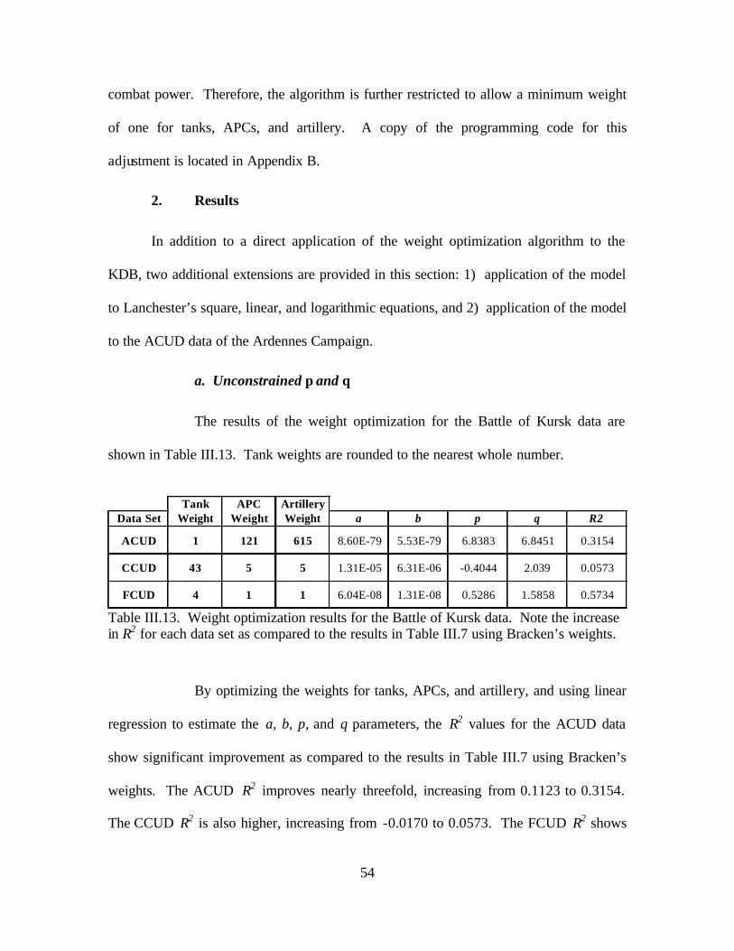
54

combat power. Therefore, the algorithm is further restricted to allow a minimum weight

of one for tanks, APCs, and artillery. A copy of the programming code for this

adjustment is located in Appendix B.

2. Results

In addition to a direct application of the weight optimization algorithm to the

KDB, two additional extensions are provided in this section: 1) application of the model

to Lanchester’s square, linear, and logarithmic equations, and 2) application of the model

to the ACUD data of the Ardennes Campaign.

a. Unconstrained p and q

The results of the weight optimization for the Battle of Kursk data are

shown in Table III.13. Tank weights are rounded to the nearest whole number.

Tank APC Artillery

Data Set Weight Weight Weight a b p q R2

ACUD 1 121 615 8.60E-79 5.53E-79 6.8383 6.8451 0.3154

CCUD 43 5 5 1.31E-05 6.31E-06 -0.4044 2.039 0.0573

FCUD 4 1 1 6.04E-08 1.31E-08 0.5286 1.5858 0.5734

Table III.13. Weight optimization results for the Battle of Kursk data. Note the increase in R2 for each data set as compared to the results in Table III.7 using Bracken’s weights.

By optimizing the weights for tanks, APCs, and artillery, and using linear

regression to estimate the a, b, p, and q parameters, the R2 values for the ACUD data

show significant improvement as compared to the results in Table III.7 using Bracken’s

weights. The ACUD R2 improves nearly threefold, increasing from 0.1123 to 0.3154.

The CCUD R2 is also higher, increasing from -0.0170 to 0.0573. The FCUD R2 shows

55

only slight improvement, increasing from 0.5541 to 0.5734. However, when compared to

the results of the combinatoric search in Table III.12, the optimization of weights has less

impact. The R2 for the ACUD data only improves from 0.2371 to 0.3154, the R2 for the

CCUD data actually decreases from 0.0607 to 0.0573, and the FCUD R2 is nearly

identical.

Although the weight optimization improves the R2 value for the ACUD

data, the resulting weights are not intuitively appealing. From most historical accounts,

the Battle of Kursk was dominated by tank battles, with APCs and artillery contributing

to a lesser degree. However, the weights for the ACUD data imply that artillery was by

far the dominant weapon on the battlefield, whereas the weights for the CCUD and

FCUD data imply that tanks were more dominant. The optimal ACUD weights appear to

be a result of Germany’s large numerical advantage in APCs and artillery and

disadvantage in manpower and tanks, shown in Figures II.2 through II.5. Upon further

inspection, the figures reveal that the Germans actually had an advantage in manpower

and tanks when considering only those forces in contact. Hence, the weighting shifts in

favor of tanks as the level of contact is narrowed from ACUD to FCUD. This effect

reflects a more accurate representation of the Battle of Kursk.

The variations in the scale of the a and b parameters is also of interest.

The a and b parameters for the ACUD data are on the scale of 1.00e-79, far smaller than

the scale for the parameters found for the CCUD and FCUD data. This correlates

negatively with the relatively high values found for the p and q parameters. In addition,

the extreme difference in scale between the parameters makes optimization more

difficult.

56

b. p and q Constrained to Linear, Square, and Logarithmic Models

In this analysis, p and q are restricted to the three basic Lanchester models,

and the weighting methodology from Chapter III.B.1 is applied to Equations III.8 through

III.13. The results of the weight optimization for the Lanchester models are shown in

Tables III.14 through III.16.

Tank APC Artillery Model Weight Weight Weight a b p q R2

Linear 1 1 1 2.11E-07 6.07E-08 1 1 0.6187

Square 1 1 1 3.35E-02 1.42E-02 1 0 0.2924

Log 6 1 1 5.22E-02 1.27E-02 0 1 0.5375

Table III.14. Weight optimization results for FCUD data with p and q restricted to Lanchester linear, square, and logarithmic models. Note the high R2 value for the linear model.


Linear 1 1 1 1.04E-07 3.05E-08 1 1 0.0619

Square 1 1 1 8.81E-02 5.39E-02 1 0 0.1281

Log 217 1 1 2.99E-02 8.39E-03 0 1 0.0126

Table III.15. Weight optimization results for CCUD data with p and q restricted to Lanchester linear, square, and logarithmic models.


Linear 55 1 226 4.97E-08 2.46E-08 1 1 0.1569

Square 479 82 61 1.17E-01 4.24E-02 1 0 0.1043

Log 1 1 1 1.93E-02 8.86E-03 0 1 0.0794

Table III.16. Weight optimization results for ACUD data with p and q restricted to Lanchester linear, square, and logarithmic models.

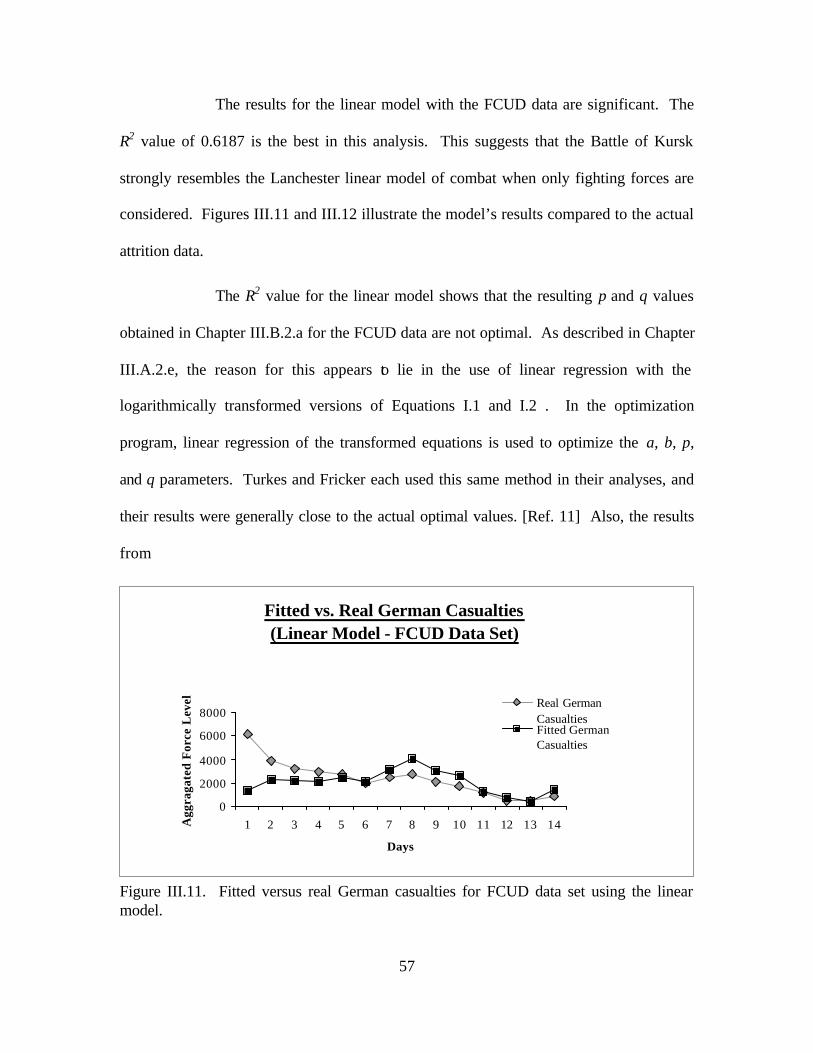
57

The results for the linear model with the FCUD data are significant. The

R2 value of 0.6187 is the best in this analysis. This suggests that the Battle of Kursk

strongly resembles the Lanchester linear model of combat when only fighting forces are

considered. Figures III.11 and III.12 illustrate the model’s results compared to the actual

attrition data.

The R2 value for the linear model shows that the resulting p and q values

obtained in Chapter III.B.2.a for the FCUD data are not optimal. As described in Chapter

III.A.2.e, the reason for this appears to lie in the use of linear regression with the

logarithmically transformed versions of Equations I.1 and I.2 . In the optimization

program, linear regression of the transformed equations is used to optimize the a, b, p,

and q parameters. Turkes and Fricker each used this same method in their analyses, and

their results were generally close to the actual optimal values. [Ref. 11] Also, the results

from

Fitted vs. Real German Casualties (Linear Model - FCUD Data Set)

0

2000

4000

6000

8000

1 2 3 4 5 6 7 8 9 10 11 12 13 14

Days

Agg

raga

ted

For

ce L

evel Real German

CasualtiesFitted GermanCasualties

Figure III.11. Fitted versus real German casualties for FCUD data set using the linear model.

58

Fitted vs. Real Soviet Casualties (Linear Model - FCUD Data Set)

0

5000

10000

15000

20000

1 2 3 4 5 6 7 8 9 10 11 12 13 14

Days

Agg

raga

ted

For

ce L

evel Real Soviet

CasualtiesFitted SovietCasualties

Figure III.12. Fitted versus real Soviet casualties for FCUD data set using the linear model.

Chapter III.A.2.c were also close to the actual optimal values, especially for the CCUD

and FCUD data. However, linear regression of the transformed data using the weights in

Table III.13 for the linear model yields a p value of 0.5259, a q value of 1.5707, and a R2

of 0.5710. Obviously, if linear regression was optimizing the p and q parameters, they

both should be closer to 1. This would yield a higher R2 and a better fitting model.

Attempts to optimize the a, b, p, and q parameters using a steepest ascent

search as described above proved unsuccessful. In this method, all seven parameters are

optimized simultaneously with no use of linear regression. However, the widely varying

scale of the individual parameters appears to be too great to enable accurate gradients to

be determined. For instance, a numerical gradient for the seven parameters requires each

parameter to be incremented by the same distance (? from the optimization algorithm).

The relative size of this distance varies greatly when compared to a weight value of 20 or

59

a b value of 1.00e-79. This creates a degree of instability between the parameters,

resulting in intuitively unappealing results (e.g. tank weights of 6000). Other factors that

adversely affect the optimization include user input values for step size and tolerance

limits. The choice of these values may slightly alter the results during each iteration of

the algorithm, ultimately affecting the final outcome.

c. Application of Model to Ardennes Campaign Data (ACUD Only)

This section applies the weighting methodology from Chapter III.B to the

ACUD data for the Ardennes Campaign (see Ref. [4]: p. 421-424). Note: Only the

ACUD data is available to the author. The intent of this section is to determine how the

model performs when compared to an alternate data set.

The first step in this analysis is to establish a baseline R2 measurement

using both linear regression on the logarithmically transformed data and the combinatoric

search method. Next, the weight optimization algorithm is applied to days two through

eleven of the data. These days represent the most intense period of fighting in the

campaign. [Ref. 4] The results of this analysis are shown in Table III.17.

Tank APC Artillery

Method Weight Weight Weight a b p q R2Linear

Regression20 5 40 9.19E+03 9.02E+03 1.6428 -1.7182 0.3232

Combinatoric Search

20 5 40 6.70E+10 1.20E+10 1.4000 -2.6000 0.5707

Weight Optimization

20 197 6 1.07E+18 9.06E+15 1.8631 -4.0347 0.6852

Table III.17. Results of Ardennes Campaign analysis. Note the large increase in R2 between the linear regression and combinatoric search methods.

60

Upon examination of the results, a similar pattern emerges when

compared to the analysis of the KDB. Linear regression of the logarithmically

transformed data provides a relatively inaccurate estimate of the optimal a, b, p and q

parameters, whereas the combinatoric search refines these estimates and results in much

higher R2. The weight optimization process improves this R2 somewhat, but the resulting

weights do not seem intuitive (i.e. APC weight of 197). Such unintuitive weighting also

occurred for the ACUD data in the KDB. Therefore, weight optimization results do not

appear to qualitatively improve the fit of the model to either the KDB or Ardennes data.

61

IV. CONCLUSIONS AND RECOMMENDATIONS A. CONCLUSIONS

The following conclusions are based on the findings in Chapter II.B.4 and the

results described in Chapters III.A.1.d, III.A.2.c, and III.B.2.

1. Data Correlations May Reflect Lanchester Models

When analyzing historical data, the correlations that exist between variables seem

to infer which Lanchester model best fits the data. Using Bracken’s weights in Chapter

II.B.4, the correlations suggested that the square model would provide the best fit for the

ACUD data, the logarithmic model would provide the best fit for the CCUD data, and the

square model would provide the best fit for the FCUD data. These predictions were

supported by the results of the linear regression analysis from Chapter III.A.2.c. In this

case, the models that best fit the ACUD, CCUD, and FCUD data agreed with the

predicted models from the correlation analysis.

2. Lanchester Models More Accurately Fit FCUD Data

In each section of analysis, the use of the FCUD data set resulted in a significantly

higher R2 value in comparison to the ACUD and CCUD data. This suggests that

Lanchester equations and their derivatives more accurately predict combat losses in cases

where only fully engaged forces are considered. This characteristic may occur more

obviously in models with large outliers, such as Day 8 in the KDB. As shown in Figures

III.1 through III.6, the major deficiency of the linear regression model when considering

the ACUD and CCUD data was the inability to account for this outlier. However, by

using FCUD data, the model better accounted for the sharp increase in casualties for this

62

day. Outliers such as these are better representations of the abnormalities that exist in

many battles. Rather than ignoring these outliers, the FCUD model may be able to deal

with them more readily.

3. FCUD Data Reveals Important Insight Concerning the Battle of Kursk

When considering all combat units, the Soviets had a consistently greater

advantage in terms of total combat power. Therefore, historical scholars have assumed

that the Germans must have been far superior in terms of training and equipment in order

to come so close to victory. Indeed, this conclusion is supported by the German’s

maintaining a higher attrition coefficient in each analysis. However, analyzing the FCUD

data reveals that the Germans actually averaged a greater number of personnel, tanks,

APCs, and artillery that were actually in contact. This indicates that the Germans had

more fighting combat power during the actual battles. Therefore, their relative success is

also supported by sheer numbers, not just by training and equipment.

4. Transformed Linear Regression Fails to Optimize p, q, a, and b in All Cases

Although Fricker and Turkes used transformed linear regression with some degree

of success in their analyses, this technique does not work well with all data sets. The

process of transforming Equations I.1 and I.2, performing linear regression, and then

converting back to the original form is somewhat unstable and only results in nearly

optimal parameter estimates. Because of this, the weighting methodology introduced in

this thesis does not optimize the a, b, p and q parameters, although it does provide the

optimal weights for given values of a, b, p and q.

63

The reason for the instability of the transformed linear regression may lie in the

different scales of the parameters being estimated. The a and b parameters are extremely

small, on the scale of 1.00 x 10-79 in the ACUD case. The p and q parameters roughly

vary between –1.00 and 5.00. Combined with a logarithmic transformation, the

optimization of these parameters with linear regression becomes less than ideal.

5. Weight Optimization Does Not Greatly Affect the Fit of Lanchester Models

Although optimizing the weights does improve the R2 statistic in some cases, this

improvement is minimal when compared to the actual optimal R2. For instance, the best

fit discovered in this analysis was with all weights set equal to one and resulted in an R2

of 0.6187. If the weights are switched to Bracken’s weights and the a, b, p, and q

parameters remain the same, the R2 decreases only slightly to 0.5513. This finding

supports the weight sensitivity analysis that Turkes performed. [Ref. 2] In addition, the

resulting weights do not always make intuitive sense without restricting their boundaries.

For instance, without restricting weights to be positive, the weight optimization program

from this analysis resulted in negative weights for all three weapon systems. This makes

no intuitive sense, indicating that increasing the amount of any weapon system actually

decreases combat power.

6. Optimized Weights FOR CCUD and FCUD Data Do Reflect Historical Accounts of the Battle of Kursk

The weights found during the weight optimization process of CCUD and FCUD

data do support historical opinion concerning the Battle of Kursk. The resulting weight

of tanks is significantly higher than the weight of personnel, artillery, and APCs. This

supports the common belief that tanks dominated the battlefield.

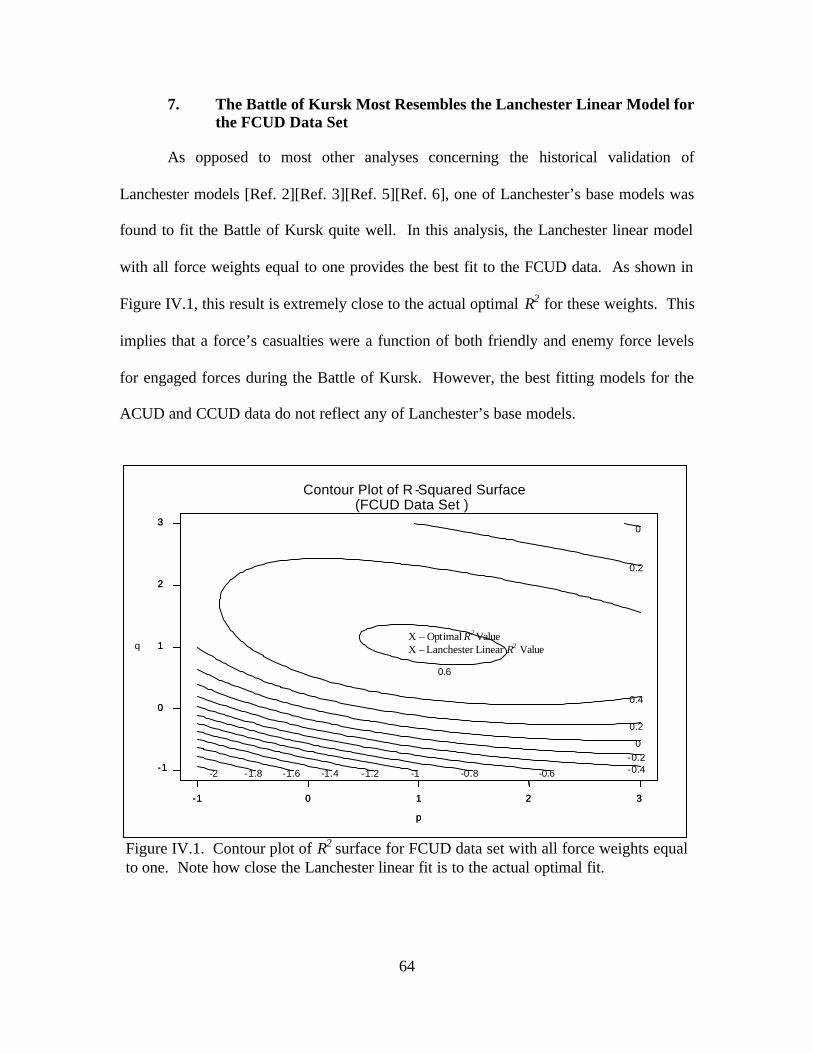
64

p

q

- 1 0 1 2 3 - 1

0

1

2

3

- 2 - 1.8 - 1.6 - 1.4 - 1.2 - 1 - 0.8 - 0.6 - 0.4 - 0.2 0

0

0.2

0.2

0.4 0.6

Contour Plot of R - Squared Surface (FCUD Data Set )

p - 1 0 1 2 3

- 1

0

1

2

3

7. The Battle of Kursk Most Resembles the Lanchester Linear Model for the FCUD Data Set

As opposed to most other analyses concerning the historical validation of

Lanchester models [Ref. 2][Ref. 3][Ref. 5][Ref. 6], one of Lanchester’s base models was

found to fit the Battle of Kursk quite well. In this analysis, the Lanchester linear model

with all force weights equal to one provides the best fit to the FCUD data. As shown in

Figure IV.1, this result is extremely close to the actual optimal R2 for these weights. This

implies that a force’s casualties were a function of both friendly and enemy force levels

for engaged forces during the Battle of Kursk. However, the best fitting models for the

ACUD and CCUD data do not reflect any of Lanchester’s base models.

X – Optimal R2 Value X – Lanchester Linear R2 Value

Figure IV.1. Contour plot of R2 surface for FCUD data set with all force weights equal to one. Note how close the Lanchester linear fit is to the actual optimal fit.

65

B. RECOMMENDATIONS FOR FURTHER RESEARCH

The following areas require additional study.

1. Extended Analysis Required for ACUD, CCUD, and FCUD Data Sets

In order to substantiate the conclusions of this thesis, additional historical data

sets must be organized into ACUD, CCUD, and FCUD subsets and analyzed to

determine the best fitting models. The Ardennes database is a prime candidate for this

type of research, given its similarity to the KDB. Analyses could include whether the

more refined data sets allow for an improved fit of the model and whether any of the base

Lanchester models fit the data well. Such analysis would assist in determining if the

conclusions above apply to other military conflicts.

2. Alternate Methods Required for Optimizing p, q, a, and b

The use of transformed linear regression to determine the optimal values of the p,

q, a, and b parameters is not ideal. In some cases, this technique worked quite well.

When using Bracken’s weights with the CCUD and FCUD data sets, the estimated values

of p, q, a, and b were quite close to the optima (see Figures III.8 and III.9). However,

with the all weights set equal to one, the estimated values were much farther from the

optima. This inconsistency is troublesome and requires the use of additional contour

surface analysis to verify that the estimated parameters from regression are indeed close

to the optima. Consequently, the development of an improved method of optimizing p, q,

a, and b simultaneously would eliminate the need for this additional step. Ideally, this

new method could be used along with the weight optimization program introduced in this

thesis to optimize all unknown parameters.

66


67

APPENDIX A. WEIGHT OPTIMIZATION PROGRAM (UNCONSTRAINED)

### All programming was completed using the S-Plus statistical package. The ### following computer code is provided as a reference only and may only prove ### useful to those parties familiar with S-Plus and the weighting optimization ### process described in Chapter III.B. All comments are in bold print. set <- dat # input data set2 <- dat2 weights <- c(1,1,1) # initialize weights Wp <- 1 Wt <- weights[1] Wapc <- weights[2] Warty <- weights[3] newparam <- regr(set,set2,Wt,Wapc,Warty) # regression to find a,b,p,q a <- newparam[1] b <- newparam[2] p <- newparam[3] q <- newparam[4] delta <- 0.1 # initialize increment distance (delta) step <- 1000 # initialize step distance (lambda) tol <- 1e-005 # initialize tolerance level epsilon <- 100 # initialize difference between initial R2

and incremented R2 while(epsilon > tol) { Wtbest <- Wt # record "best" weights Wapcbest <- Wapc Wartybest <- Warty r2next <- 1 # initialize r2next, r2now, lambda r2now <- 0 lambda <- 10000 diff <- 100 # diff = difference between new R2 and initial R2 r2init <- rsquare(set, c(Wp, Wt, Wapc, Warty, a, b, p, q)) # calculate

initial R2 ####Calculate partial derivatives newparam <- regr(set, set2, Wt + delta, Wapc, Warty) # regression to

find a,b,p,q a <- newparam[1] b <- newparam[2] p <- newparam[3] q <- newparam[4] wtderiv <- (rsquare(set, c(Wp, Wt + delta, Wapc, Warty, a, b, p, q)) -

r2init)/delta # partial derivative with respect to tank weight newparam <- regr(set, set2, Wt, Wapc + delta, Warty) # regression to

find a,b,p,q a <- newparam[1] b <- newparam[2] p <- newparam[3] q <- newparam[4] wapcderiv <- (rsquare(set, c(Wp, Wt, Wapc + delta, Warty, a, b, p, q)) -

r2init)/delta # partial derivative with respect to APC weight newparam <- regr(set, set2, Wt, Wapc, Warty + delta) # regression to

find a,b,p,q a <- newparam[1] b <- newparam[2] p <- newparam[3]

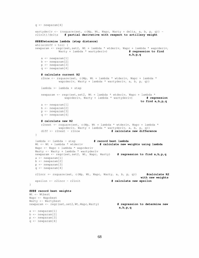
68

q <- newparam[4] wartyderiv <- (rsquare(set, c(Wp, Wt, Wapc, Warty + delta, a, b, p, q)) -

r2init)/delta # partial derivative with respect to artillery weight ####Determine lambda (step distance) while(diff > tol) { newparam <- regr(set,set2, Wt + lambda * wtderiv, Wapc + lambda * wapcderiv, Warty + lambda * wartyderiv) # regression to find a,b,p,q a <- newparam[1] b <- newparam[2] p <- newparam[3] q <- newparam[4] # calculate current R2 r2now <- rsquare(set, c(Wp, Wt + lambda * wtderiv, Wapc + lambda * wapcderiv, Warty + lambda * wartyderiv, a, b, p, q)) lambda <- lambda + step newparam <- regr(set,set2, Wt + lambda * wtderiv, Wapc + lambda * wapcderiv, Warty + lambda * wartyderiv) # regression to find a,b,p,q a <- newparam[1] b <- newparam[2] p <- newparam[3] q <- newparam[4] # calculate new R2 r2next <- rsquare(set, c(Wp, Wt + lambda * wtderiv, Wapc + lambda * wapcderiv, Warty + lambda * wartyderiv, a, b, p, q)) diff <- r2next - r2now # calculate new difference } lambda <- lambda - step # record best lambda Wt <- Wt + lambda * wtderiv # calculate new weights using lambda Wapc <- Wapc + lambda * wapcderiv Warty <- Warty + lambda * wartyderiv newparam <- regr(set,set2, Wt, Wapc, Warty) # regression to find a,b,p,q a <- newparam[1] b <- newparam[2] p <- newparam[3] q <- newparam[4] r2incr <- rsquare(set, c(Wp, Wt, Wapc, Warty, a, b, p, q)) #calculate R2

with new weights epsilon <- r2incr - r2init # calculate new epsilon } #### record best weights Wt <- Wtbest Wapc <- Wapcbest Warty <- Wartybest newparam <- regr(set,set2,Wt,Wapc,Warty) # regression to determine new a,b,p,q a <- newparam[1] b <- newparam[2] p <- newparam[3] q <- newparam[4]

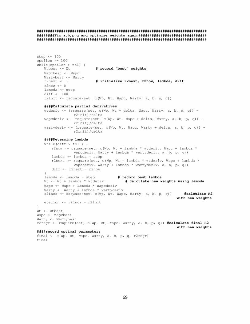
69

############################################################################# ########Fix a,b,p,q and optimize weights again############################### ############################################################################# step <- 100 epsilon <- 100 while(epsilon > tol) { Wtbest <- Wt # record "best" weights Wapcbest <- Wapc Wartybest <- Warty r2next <- 1 # initialize r2next, r2now, lambda, diff r2now <- 0 lambda <- step diff <- 100 r2init <- rsquare(set, c(Wp, Wt, Wapc, Warty, a, b, p, q)) ####Calculate partial derivatives wtderiv <- (rsquare(set, c(Wp, Wt + delta, Wapc, Warty, a, b, p, q)) – r2init)/delta wapcderiv <- (rsquare(set, c(Wp, Wt, Wapc + delta, Warty, a, b, p, q)) – r2init)/delta wartyderiv <- (rsquare(set, c(Wp, Wt, Wapc, Warty + delta, a, b, p, q)) – r2init)/delta ####Determine lambda while(diff > tol ) { r2now <- rsquare(set, c(Wp, Wt + lambda * wtderiv, Wapc + lambda * wapcderiv, Warty + lambda * wartyderiv, a, b, p, q)) lambda <- lambda + step r2next <- rsquare(set, c(Wp, Wt + lambda * wtderiv, Wapc + lambda * wapcderiv, Warty + lambda * wartyderiv, a, b, p, q)) diff <- r2next - r2now } lambda <- lambda - step # record best lambda Wt <- Wt + lambda * wtderiv # calculate new weights using lambda Wapc <- Wapc + lambda * wapcderiv Warty <- Warty + lambda * wartyderiv r2incr <- rsquare(set, c(Wp, Wt, Wapc, Warty, a, b, p, q)) #calculate R2 with new weights epsilon <- r2incr - r2init } Wt <- Wtbest Wapc <- Wapcbest Warty <- Wartybest r2regr <- rsquare(set, c(Wp, Wt, Wapc, Warty, a, b, p, q)) #calculate final R2 with new weights ####record optimal parameters final <- c(Wp, Wt, Wapc, Warty, a, b, p, q, r2regr) final

70


71

APPENDIX B. WEIGHT OPTIMIZATION PROGRAM (CONSTRAINED TO POSITIVE WEIGHTS)

### All programming was completed using the S-Plus statistical package. The ### following computer code is provided as a reference only and may only prove ### useful to those parties familiar with S-Plus and the weighting optimization ### process described in Chapter III.B. All comments are in bold print. set <- dat # input data set2 <- dat2 weights <- c(1,1,1) # initialize weights Wp <- 1 Wt <- weights[1] Wapc <- weights[2] Warty <- weights[3] newparam <- regr(set,set2,Wt,Wapc,Warty) # regression to find a,b,p,q a <- newparam[1] b <- newparam[2] p <- newparam[3] q <- newparam[4] delta <- .1 # initialize increment distance (delta) step <- 1000 # initialize step distance (lambda) tol <- 1e-005 # initialize tolerance level epsilon <- 100 # initialize difference between initial R2 and

incremented R2 (epsilon) while(epsilon > tol) { Wtbest <- Wt # record "best" weights Wapcbest <- Wapc Wartybest <- Warty WtNew <- 0 # initialize temp variables WapcNew <- 0 WartyNew <- 0 r2next <- 1 # initialize r2next, r2now, lambda, diff r2now <- 0 lambda <- step diff <- 100 # diff = difference between new R2 and initial R2 r2init <- rsquare(set, c(Wp, Wt, Wapc, Warty, a, b, p, q)) # calculate

initial R2 ####Calculate partial derivatives newparam <- regr(set, set2, Wt + delta, Wapc, Warty) # regression to find a,b,p,q a <- newparam[1] b <- newparam[2] p <- newparam[3] q <- newparam[4] wtderiv <- (rsquare(set, c(Wp, Wt + delta, Wapc, Warty, a, b, p, q)) -

r2init)/delta # partial derivative with respect to tank weight newparam <- regr(set, set2, Wt, Wapc + delta, Warty) # regression to find a,b,p,q a <- newparam[1] b <- newparam[2] p <- newparam[3] q <- newparam[4] wapcderiv <- (rsquare(set, c(Wp, Wt, Wapc + delta, Warty, a, b, p, q)) -

r2init)/delta # partial derivative with respect to APC weight newparam <- regr(set, set2, Wt, Wapc, Warty + delta) # regression to find a,b,p,q a <- newparam[1]

72

b <- newparam[2] p <- newparam[3] q <- newparam[4] wartyderiv <- (rsquare(set, c(Wp, Wt, Wapc, Warty + delta, a, b, p, q)) -

r2init)/delta # partial derivative with respect to artillery weight ####Determine lambda and new weights (numbers indicate required logic tests) ###1 – all partial derivatives positive if(wtderiv > 0 && wapcderiv > 0 && wartyderiv > 0) { while(diff > tol ) {

newparam <- regr(set,set2, Wt + lambda * wtderiv, Wapc + lambda * wapcderiv, Warty + lambda * wartyderiv) # regression to find a,b,p,q

a <- newparam[1] b <- newparam[2] p <- newparam[3] q <- newparam[4]

r2now <- rsquare(set, c(Wp, Wt + lambda * wtderiv, Wapc + lambda * wapcderiv, Warty + lambda * wartyderiv, a, b, p, q))

lambda <- lambda + step



r2next <- rsquare(set, c(Wp, Wt + lambda * wtderiv, Wapc + lambda * wapcderiv, Warty + lambda * wartyderiv, a, b, p, q))

diff <- r2next - r2now } lambda <- lambda - step # record best lambda Wt <- Wt + lambda * wtderiv # calculate new weights using lambda Wapc <- Wapc + lambda * wapcderiv Warty <- Warty + lambda * wartyderiv newparam <- regr(set,set2, Wt, Wapc, Warty) # regression to find a,b,p,q a <- newparam[1] b <- newparam[2] p <- newparam[3] q <- newparam[4] r2incr <- rsquare(set, c(Wp, Wt, Wapc, Warty, a, b, p, q)) #calculate R2

with new weights epsilon <- r2incr - r2init } ### 2 – negative partial derivative for artillery if(wtderiv > 0 && wapcderiv > 0 && wartyderiv < 0) { WartyTemp <- Warty + lambda * wartyderiv # record temporary weight while(diff > tol && WartyTemp > 1) {




lambda <- lambda + step newparam <- regr(set,set2, Wt + lambda * wtderiv, Wapc + lambda *

wapcderiv, Warty + lambda * wartyderiv) # regression to find a,b,p,q a <- newparam[1]

73

b <- newparam[2] p <- newparam[3] q <- newparam[4]


diff <- r2next - r2now WartyTemp <- Warty + lambda * wartyderiv } while(diff > tol && WartyTemp <= 1) { Warty <- 1

newparam <- regr(set,set2, Wt + lambda * wtderiv, Wapc + lambda * wapcderiv, Warty) # regression to find a,b,p,q


r2now <- rsquare(set, c(Wp, Wt + lambda * wtderiv, Wapc + lambda * wapcderiv, Warty, a, b, p, q))


wapcderiv, Warty) # regression to find a,b,p,q a <- newparam[1] b <- newparam[2] p <- newparam[3] q <- newparam[4]

r2next <- rsquare(set, c(Wp, Wt + lambda * wtderiv, Wapc + lambda * wapcderiv, Warty, a, b, p, q))

diff <- r2next - r2now } lambda <- lambda - step # record best lambda Wt <- Wt + lambda * wtderiv # calculate new weights using lambda Wapc <- Wapc + lambda * wapcderiv WartyNew <- Warty + lambda * wartyderiv if (WartyNew > 1) { Warty <- Warty + lambda * wartyderiv } if (WartyNew <= 1) { Warty <- 1 } newparam <- regr(set,set2, Wt, Wapc, Warty) # regression to find a,b,p,q a <- newparam[1] b <- newparam[2] p <- newparam[3] q <- newparam[4] r2incr <- rsquare(set, c(Wp, Wt, Wapc, Warty, a, b, p, q))

#calculate R2 with new weights epsilon <- r2incr - r2init } ###3 – negative partial derivative for APCs if(wtderiv > 0 && wartyderiv > 0 && wapcderiv < 0) { WapcTemp <- Wapc + lambda * wapcderiv while(diff > tol && WapcTemp > 1) {





wapcderiv, Warty + lambda * wartyderiv) # regression to find a,b,p,q

74



diff <- r2next - r2now WapcTemp <- Wapc + lambda * wapcderiv } while(diff > tol && WapcTemp <= 1 ) { Wapc <- 1

newparam <- regr(set,set2, Wt + lambda * wtderiv, , Warty + lambda * wartyderiv) # regression to find a,b,p,q

a <- newparam[1] b <- newparam[2] p <- newparam[3] q <- newparam[4] r2now <- rsquare(set, c(Wp, Wt + lambda * wtderiv, Wapc, Warty + lambda * wartyderiv, a, b, p, q)) lambda <- lambda + step

newparam <- regr(set,set2, Wt + lambda * wtderiv, Wapc, Warty + lambda * wartyderiv) # regression to find a,b,p,q

a <- newparam[1] b <- newparam[2] p <- newparam[3] q <- newparam[4] r2next <- rsquare(set, c(Wp, Wt + lambda * wtderiv, Wapc, Warty + lambda * wartyderiv, a, b, p, q)) diff <- r2next - r2now } lambda <- lambda - step # record best lambda Wt <- Wt + lambda * wtderiv # calculate new weights using lambda Warty <- Warty + lambda * wartyderiv WapcNew <- Wapc + lambda * wapcderiv if (WapcNew > 1) { Wapc <- Wapc + lambda * wapcderiv } if (WapcNew <= 1) { Wapc <- 1 } newparam <- regr(set,set2, Wt, Wapc, Warty) # regression to find a,b,p,q a <- newparam[1] b <- newparam[2] p <- newparam[3] q <- newparam[4] r2incr <- rsquare(set, c(Wp, Wt, Wapc, Warty, a, b, p, q)) #calculate R2 with new weights epsilon <- r2incr - r2init } ###4 – negative partial derivative for tanks if(wapcderiv > 0 && wartyderiv > 0 && wtderiv < 0) { WtTemp <- Wt + lambda * wtderiv while(diff > tol && WtTemp > 1) {




WtNew <- Wt + lambda * wtderiv lambda <- lambda + step

75




diff <- r2next - r2now WtTemp <- Wt + lambda * wtderiv } while(diff > tol && WtTemp <= 1) { Wt <- 1

newparam <- regr(set,set2, Wt, Wapc + lambda * wapcderiv, Warty + lambda * wartyderiv) # regression to find a,b,p,q

a <- newparam[1] b <- newparam[2] p <- newparam[3] q <- newparam[4] r2now <- rsquare(set, c(Wp, Wt, Wapc + lambda * wapcderiv, Warty + lambda * wartyderiv, a, b, p, q)) lambda <- lambda + step


a <- newparam[1] b <- newparam[2] p <- newparam[3] q <- newparam[4] r2next <- rsquare(set, c(Wp, Wt, Wapc + lambda * wapcderiv, Warty + lambda * wartyderiv, a, b, p, q)) diff <- r2next - r2now } lambda <- lambda - step # record best lambda WtNew <- Wt + lambda * wtderiv Wapc <- Wapc + lambda * wapcderiv Warty <- Warty + lambda * wartyderiv if (WtNew > 1) { Wt <- Wt + lambda * wtderiv } if (WtNew <= 1) { Wt <- 1 } newparam <- regr(set,set2, Wt, Wapc, Warty) #regression to find a,b,p,q a <- newparam[1] b <- newparam[2] p <- newparam[3] q <- newparam[4] r2incr <- rsquare(set, c(Wp, Wt, Wapc, Warty, a, b, p, q))#calculate R2 with new weights epsilon <- r2incr - r2init } ###5 – negative partial derivative for APCs and artillery if(wtderiv > 0 && wapcderiv < 0 && wartyderiv < 0) { WapcTemp <- Wapc + lambda * wapcderiv WartyTemp <- Warty + lambda * wartyderiv while(diff > tol && WapcTemp > 1 && WartyTemp > 1) {



76

r2now <- rsquare(set, c(Wp, Wt + lambda * wtderiv, Wapc+ lambda * wapcderiv, Warty +lambda * wartyderiv, a, b, p, q))

WapcNew <- Wapc + lambda * wapcderiv WartyNew <- Warty + lambda * wartyderiv lambda <- lambda + step



r2next <- rsquare(set, c(Wp, Wt + lambda * wtderiv, Wapc+ lambda * wapcderiv, Warty +lambda * wartyderiv, a, b, p, q))

diff <- r2next - r2now WapcTemp <- Wapc + lambda * wapcderiv WartyTemp <- Warty + lambda * wartyderiv } while(diff > tol && WapcTemp <= 1 && WartyTemp > 1) { Wapc <- 1


a <- newparam[1] b <- newparam[2] p <- newparam[3] q <- newparam[4] r2now <- rsquare(set, c(Wp, Wt + lambda * wtderiv, Wapc, Warty + lambda * wartyderiv, a, b, p, q)) WartyNew <- Warty + lambda * wartyderiv lambda <- lambda + step


a <- newparam[1] b <- newparam[2] p <- newparam[3] q <- newparam[4] r2next <- rsquare(set, c(Wp, Wt + lambda * wtderiv, Wapc, Warty + lambda * wartyderiv, a, b, p, q)) diff <- r2next - r2now WartyTemp <- Warty + lambda * wartyderiv } while(diff > tol && WapcTemp > 1 && WartyTemp <= 1) { Warty <- 1



r2now <- rsquare(set, c(Wp, Wt + lambda * wtderiv, Wapc+ lambda * wapcderiv, Warty,a, b, p, q))

WapcNew <- Wapc + lambda * wapcderiv lambda <- lambda + step



r2next <- rsquare(set, c(Wp, Wt + lambda * wtderiv, Wapc+ lambda * wapcderiv, Warty, a, b, p, q))

diff <- r2next - r2now WapcTemp <- Wapc + lambda * wapcderiv }

77

while(diff > tol && WapcTemp <= 1 && WartyTemp <= 1) { Wapc <- 1 Warty <- 1 newparam <- regr(set,set2, Wt + lambda * wtderiv, Wapc, Warty) #regression to find a,b,p,q a <- newparam[1] b <- newparam[2] p <- newparam[3] q <- newparam[4]

r2now <- rsquare(set, c(Wp, Wt + lambda * wtderiv, Wapc, Warty , a, b, p, q))

lambda <- lambda + step newparam <- regr(set,set2, Wt + lambda * wtderiv, Wapc, Warty) #regression to find a,b,p,q a <- newparam[1] b <- newparam[2] p <- newparam[3] q <- newparam[4]

r2next <- rsquare(set, c(Wp, Wt + lambda * wtderiv, Wapc, Warty , a, b, p, q))

diff <- r2next - r2now } lambda <- lambda - step # record best lambda Wt <- Wt + lambda * wtderiv # calculate new weights using lambda WapcNew <- Wapc + lambda * wapcderiv WartyNew <- Warty + lambda * wartyderiv if (WapcNew > 1) { Wapc <- Wapc + lambda * wapcderiv } if (WartyNew > 1) { Warty <- Warty + lambda * wartyderiv } if (WapcNew <= 1) { Wapc <- 1 } if (WartyNew <= 1) { Warty <- 1 } newparam <- regr(set,set2, Wt, Wapc, Warty) # regression to find a,b,p,q a <- newparam[1] b <- newparam[2] p <- newparam[3] q <- newparam[4] r2incr <- rsquare(set, c(Wp, Wt, Wapc, Warty, a, b, p, q))

#calculate R2 with new weights epsilon <- r2incr - r2init } ###6 – negative partial derivative for APCs and tanks if(wtderiv < 0 && wapcderiv < 0 && wartyderiv > 0) { WtTemp <- Wt + lambda * wtderiv WapcTemp <- Wapc + lambda * wapcderiv while(diff > tol && WtTemp > 1 && WapcTemp > 1 ) {

newparam <- regr(set,set2, Wt + lambda * wtderiv, Wapc + lambda * wapcderiv, Warty + lambda * wartyderiv) # regression to find

a,b,p,q a <- newparam[1] b <- newparam[2] p <- newparam[3] q <- newparam[4]

r2now <- rsquare(set, c(Wp, Wt+ lambda * wtderiv, Wapc + lambda * wapcderiv, Warty + lambda * wartyderiv, a, b, p, q))

WtNew <- Wt + lambda * wtderiv

78





diff <- r2next - r2now WtTemp <- Wt + lambda * wtderiv WapcTemp <- Wapc + lambda * wapcderiv } while(diff > tol && WtTemp > 1 && WapcTemp <= 1) { Wapc <- 1


a <- newparam[1] b <- newparam[2] p <- newparam[3] q <- newparam[4] r2now <- rsquare(set, c(Wp, Wt + lambda * wtderiv, Wapc, Warty + lambda * wartyderiv, a, b, p, q)) WtNew <- Wt + lambda * wtderiv lambda <- lambda + step


a <- newparam[1] b <- newparam[2] p <- newparam[3] q <- newparam[4] r2next <- rsquare(set, c(Wp, Wt + lambda * wtderiv, Wapc, Warty + lambda * wartyderiv, a, b, p, q)) diff <- r2next - r2now WtTemp <- Wt + lambda * wtderiv } while(diff > tol && WtTemp <= 1 && WapcTemp > 1) { Wt <- 1


a <- newparam[1] b <- newparam[2] p <- newparam[3] q <- newparam[4] r2now <- rsquare(set, c(Wp, Wt, Wapc + lambda * wapcderiv, Warty + lambda * wartyderiv, a, b, p, q)) WapcNew <- Wapc + lambda * wapcderiv lambda <- lambda + step


a <- newparam[1] b <- newparam[2] p <- newparam[3] q <- newparam[4] r2next <- rsquare(set, c(Wp, Wt, Wapc + lambda * wapcderiv, Warty + lambda * wartyderiv, a, b, p, q)) diff <- r2next - r2now WapcTemp <- Wapc + lambda * wapcderiv } while(diff > tol && WtTemp <= 1 && WapcTemp <= 1 ) { Wt <- 1

79

Wapc <- 1 newparam <- regr(set,set2, Wt, Wapc, Warty + lambda * wartyderiv) # regression to find a,b,p,q a <- newparam[1] b <- newparam[2] p <- newparam[3] q <- newparam[4]

r2now <- rsquare(set, c(Wp, Wt, Wapc, Warty + lambda * wartyderiv, a, b, p, q))

lambda <- lambda + step newparam <- regr(set,set2, Wt, Wapc, Warty + lambda * wartyderiv) # regression to find a,b,p,q a <- newparam[1] b <- newparam[2] p <- newparam[3] q <- newparam[4]

r2next <- rsquare(set, c(Wp, Wt, Wapc, Warty + lambda * wartyderiv, a, b, p, q))

diff <- r2next - r2now } lambda <- lambda - step # record best lambda WtNew <- Wt + lambda * wtderiv WapcNew <- Wapc + lambda * wapcderiv Warty <- Warty + lambda * wartyderiv # calculate new weights using lambda if (WapcNew > 1) { Wapc <- Wapc + lambda * wapcderiv } if (WtNew > 1) { Wt <- Wt + lambda * wtderiv } if (WapcNew <= 1) { Wapc <- 1 } if (WtNew <= 1) { Wt <- 1 } newparam <- regr(set,set2, Wt, Wapc , Warty) # regression to find a,b,p,q a <- newparam[1] b <- newparam[2] p <- newparam[3] q <- newparam[4] r2incr <- rsquare(set, c(Wp, Wt, Wapc, Warty, a, b, p, q)) #calculate R2 with new weights epsilon <- r2incr - r2init } ###7 – negative partial derivative for tanks and artillery if(wtderiv < 0 && wapcderiv > 0 && wartyderiv < 0) { WtTemp <- Wt + lambda * wtderiv WartyTemp <- Warty + lambda * wartyderiv while(diff > tol && WtTemp > 1 && WartyTemp > 1 ) {


a,b,p,q a <- newparam[1] b <- newparam[2] p <- newparam[3] q <- newparam[4] r2now <- rsquare(set, c(Wp, Wt+ lambda * wtderiv, Wapc + lambda * wapcderiv, Warty + lambda * wartyderiv, a, b, p, q)) WtNew <- Wt + lambda * wtderiv WartyNew <- Warty + lambda * wartyderiv lambda <- lambda + step

80


a <- newparam[1] b <- newparam[2] p <- newparam[3] q <- newparam[4] r2next <- rsquare(set, c(Wp, Wt + lambda * wtderiv, Wapc + lambda * wapcderiv, Warty + lambda * wartyderiv, a, b, p, q)) diff <- r2next - r2now WtTemp <- Wt + lambda * wtderiv WartyTemp <- Warty + lambda * wartyderiv } while(diff > tol && WtTemp > 1 && WartyTemp <= 1) { Warty <- 1 newparam <- regr(set,set2, Wt + lambda * wtderiv, Wapc + lambda * wapcderiv, Warty) # regression to find a,b,p,q a <- newparam[1] b <- newparam[2] p <- newparam[3] q <- newparam[4]






diff <- r2next - r2now WtTemp <- Wt + lambda * wtderiv } while(diff > tol && WtTemp <= 1 && WartyTemp > 1) { Wt <- 1


a <- newparam[1] b <- newparam[2] p <- newparam[3] q <- newparam[4] r2now <- rsquare(set, c(Wp, Wt, Wapc + lambda * wapcderiv, Warty + lambda * wartyderiv, a, b, p, q)) WartyNew <- Warty + lambda * wartyderiv lambda <- lambda + step


a <- newparam[1] b <- newparam[2] p <- newparam[3] q <- newparam[4] r2next <- rsquare(set, c(Wp, Wt, Wapc + lambda * wapcderiv, Warty + lambda * wartyderiv, a, b, p, q)) diff <- r2next - r2now WartyTemp <- Warty + lambda * wartyderiv } while(diff > tol && WtTemp <= 1 && WartyTemp <= 1 ) { Wt <- 1 Warty <- 1 newparam <- regr(set,set2, Wt, Wapc + lambda * wapcderiv, Warty ) # regression to find a,b,p,q

81


r2now <- rsquare(set, c(Wp, Wt, Wapc + lambda * wapcderiv, Warty, a, b, p, q))

lambda <- lambda + step newparam <- regr(set,set2, Wt, Wapc + lambda * wapcderiv, Warty) # regression to find a,b,p,q a <- newparam[1] b <- newparam[2] p <- newparam[3] q <- newparam[4]

r2next <- rsquare(set, c(Wp, Wt, Wapc + lambda * wapcderiv, Warty, a, b, p, q))

diff <- r2next - r2now } lambda <- lambda - step # record best lambda WtNew <- Wt + lambda * wtderiv Wapc <- Wapc + lambda * wapcderiv WartyNew <- Warty + lambda * wartyderiv if (WartyNew > 1) { Warty <- Warty + lambda * wartyderiv } if (WtNew > 1) { Wt <- Wt + lambda * wtderiv } if (WartyNew <= 1) { Warty <- 1 } if (WtNew <= 1) { Wt <- 1 } newparam <- regr(set,set2, Wt, Wapc, Warty) # regression to find a,b,p,q a <- newparam[1] b <- newparam[2] p <- newparam[3] q <- newparam[4] r2incr <- rsquare(set, c(Wp, Wt, Wapc, Warty, a, b, p, q))

#calculate R2 with new weights epsilon <- r2incr - r2init } ###8 – all partial derivatives are negative if(wtderiv < 0 && wapcderiv < 0 && wartyderiv < 0) { WtTemp <- Wt + lambda * wtderiv WapcTemp <- Wapc + lambda * wapcderiv WartyTemp <- Warty + lambda * wartyderiv while(diff > tol && WtTemp > 1 && WapcTemp > 1 && WartyTemp > 1 ) {




WtNew <- Wt + lambda * wtderiv WapcNew <- Wapc + lambda * wapcderiv WartyNew <- Warty + lambda * wartyderiv lambda <- lambda + step

82




diff <- r2next - r2now WtTemp <- Wt + lambda * wtderiv WapcTemp <- Wapc + lambda * wapcderiv WartyTemp <- Warty + lambda * wartyderiv } while(diff > tol && WtTemp > 1 && WapcTemp > 1 && WartyTemp <= 1 ) { Warty <- 1


a <- newparam[1] b <- newparam[2] p <- newparam[3] q <- newparam[4] r2now <- rsquare(set, c(Wp, Wt+ lambda * wtderiv, Wapc + lambda * wapcderiv, Warty, a, b, p, q)) WtNew <- Wt + lambda * wtderiv WapcNew <- Wapc + lambda * wapcderiv lambda <- lambda + step




diff <- r2next - r2now WtTemp <- Wt + lambda * wtderiv WapcTemp <- Wapc + lambda * wapcderiv } while(diff > tol && WtTemp > 1 && WapcTemp <= 1 && WartyTemp > 1 ) { Wapc <- 1 newparam <- regr(set,set2, Wt + lambda * wtderiv, Wapc, Warty + lambda * wartyderiv) # regression to find a,b,p,q a <- newparam[1] b <- newparam[2] p <- newparam[3] q <- newparam[4] r2now <- rsquare(set, c(Wp, Wt+ lambda * wtderiv, Wapc, Warty + lambda * wartyderiv, a, b, p, q)) WtNew <- Wt + lambda * wtderiv WartyNew <- Warty + lambda * wartyderiv lambda <- lambda + step newparam <- regr(set,set2, Wt + lambda * wtderiv, Wapc , Warty + lambda * wartyderiv) # regression to find a,b,p,q a <- newparam[1] b <- newparam[2] p <- newparam[3] q <- newparam[4] r2next <- rsquare(set, c(Wp, Wt + lambda * wtderiv, Wapc, Warty + lambda * wartyderiv, a, b, p, q)) diff <- r2next - r2now WtTemp <- Wt + lambda * wtderiv WartyTemp <- Warty + lambda * wartyderiv

83

} while(diff > tol && WtTemp <= 1 && WapcTemp > 1 && WartyTemp > 1 ) { Wt <- 1 newparam <- regr(set,set2, Wt, Wapc + lambda * wapcderiv, Warty + lambda * wartyderiv) # regression to find a,b,p,q a <- newparam[1] b <- newparam[2] p <- newparam[3] q <- newparam[4] r2now <- rsquare(set, c(Wp, Wt, Wapc + lambda * wapcderiv, Warty + lambda * wartyderiv, a, b, p, q)) WapcNew <- Wapc + lambda * wapcderiv WartyNew <- Warty + lambda * wartyderiv lambda <- lambda + step newparam <- regr(set,set2, Wt, Wapc + lambda * wapcderiv, Warty + lambda * wartyderiv) # regression to find a,b,p,q a <- newparam[1] b <- newparam[2] p <- newparam[3] q <- newparam[4] r2next <- rsquare(set, c(Wp, Wt, Wapc + lambda * wapcderiv, Warty + lambda * wartyderiv, a, b, p, q)) diff <- r2next - r2now WapcTemp <- Wapc + lambda * wapcderiv WartyTemp <- Warty + lambda * wartyderiv } while(diff > tol && WtTemp > 1 && WapcTemp <= 1 && WartyTemp <= 1 ) { Wapc <- 1 Warty <- 1 newparam <- regr(set,set2, Wt + lambda * wtderiv, Wapc, Warty) # regression to find a,b,p,q a <- newparam[1] b <- newparam[2] p <- newparam[3] q <- newparam[4]

r2now <- rsquare(set, c(Wp, Wt+ lambda * wtderiv, Wapc, Warty, a, b, p, q))


newparam <- regr(set,set2, Wt + lambda * wtderiv, Wapc , Warty) #regression to find a,b,p,q


r2next <- rsquare(set, c(Wp, Wt+ lambda * wtderiv, Wapc, Warty, a, b, p, q))

diff <- r2next - r2now WtTemp <- Wt + lambda * wtderiv } while(diff > tol && WtTemp <= 1 && WapcTemp > 1 && WartyTemp <= 1 ) { Wt <- 1 Warty <- 1 newparam <- regr(set,set2, Wt, Wapc + lambda * wapcderiv, Warty) # regression to find a,b,p,q a <- newparam[1] b <- newparam[2] p <- newparam[3] q <- newparam[4]



84

newparam <- regr(set,set2, Wt, Wapc + lambda * wapcderiv, Warty) # regression to find a,b,p,q a <- newparam[1] b <- newparam[2] p <- newparam[3] q <- newparam[4]


diff <- r2next - r2now WapcTemp <- Wapc + lambda * wapcderiv } while(diff > tol && WtTemp <= 1 && WapcTemp <= 1 && WartyTemp > 1 ) { Wt <- 1 Wapc <- 1 newparam <- regr(set,set2, Wt, Wapc, Warty + lambda * wartyderiv) # regression to find a,b,p,q a <- newparam[1] b <- newparam[2] p <- newparam[3] q <- newparam[4]


WartyNew <- Warty + lambda * wartyderiv lambda <- lambda + step newparam <- regr(set,set2, Wt, Wapc, Warty + lambda * wartyderiv) # regression to find a,b,p,q a <- newparam[1] b <- newparam[2] p <- newparam[3] q <- newparam[4]


diff <- r2next - r2now WartyTemp <- Warty + lambda * wartyderiv } if(diff > tol && WtTemp <= 1 && WapcTemp <= 1 && WartyTemp <= 1 ) { Wt <- 1 Wapc <- 1 Warty <- 1 } lambda <- lambda - step WtNew <- Wt + lambda * wtderiv WapcNew <- Wapc + lambda * wapcderiv WartyNew <- Warty + lambda * wartyderiv if (WapcNew > 1) { Wapc <- Wapc + lambda * wapcderiv } if (WartyNew > 1) { Warty <- Warty + lambda * wartyderiv } if (WtNew > 1) { Wt <- Wt + lambda * wtderiv } if (WapcNew <= 1) { Wapc <- 1 } if (WartyNew <= 1) { Warty <- 1 } if (WtNew <= 1) { Wt <- 1 }

85

newparam <- regr(set,set2, Wt, Wapc, Warty) # regression to find a,b,p,q a <- newparam[1] b <- newparam[2] p <- newparam[3] q <- newparam[4] r2incr <- rsquare(set, c(Wp, Wt, Wapc, Warty, a, b, p, q)) #calculate R2 with new weights epsilon <- r2incr - r2init } } ############################################################################### ######Fix a,b,p,q and optimize weights######################################### ############################################################################### ####record best weights Wt <- Wtbest Wapc <- Wapcbest Warty <- Wartybest newparam <- regr(set,set2,Wt,Wapc,Warty) # regression to determine new a,b,p,q a <- newparam[1] b <- newparam[2] p <- newparam[3] q <- newparam[4] step <- 100 epsilon <- 100 while(epsilon > tol) { Wtbest <- Wt # record "best" weights Wapcbest <- Wapc Wartybest <- Warty WtNew <- 0 WapcNew <- 0 WartyNew <- 0 r2next <- 1 # initialize r2next, r2now, lambda r2now <- 0 lambda <- step diff <- 100 # diff = difference between new R2 and initial R2 r2init <- rsquare(set, c(Wp, Wt, Wapc, Warty, a, b, p, q)) ####Calculate partial derivatives wtderiv <- (rsquare(set, c(Wp, Wt + delta, Wapc, Warty, a, b, p, q)) -

r2init)/delta wapcderiv <- (rsquare(set, c(Wp, Wt, Wapc + delta, Warty, a, b, p, q)) -

r2init)/delta wartyderiv <- (rsquare(set, c(Wp, Wt, Wapc, Warty + delta, a, b, p, q)) -

r2init)/delta ####Determine lambda ##1 – all partial derivatives positive if(wtderiv > 0 && wapcderiv > 0 && wartyderiv > 0) { while(diff > tol ) {


lambda <- lambda + step r2next <- rsquare(set, c(Wp, Wt + lambda * wtderiv, Wapc + lambda *

wapcderiv, Warty + lambda * wartyderiv, a, b, p, q)) diff <- r2next - r2now }

86

lambda <- lambda - step # record best lambda Wt <- Wt + lambda * wtderiv # calculate new weights using lambda Wapc <- Wapc + lambda * wapcderiv Warty <- Warty + lambda * wartyderiv r2incr <- rsquare(set, c(Wp, Wt, Wapc, Warty, a, b, p, q)) #calculate R2 with new weights epsilon <- r2incr - r2init } ### 2 – negative partial derivative for artillery if(wtderiv > 0 && wapcderiv > 0 && wartyderiv < 0) { WartyTemp <- Warty + lambda * wartyderiv while(diff > tol && WartyTemp > 1) {


WartyNew <- Warty + lambda * wartyderiv lambda <- lambda + step


diff <- r2next - r2now WartyTemp <- Warty + lambda * wartyderiv } while(diff > tol && WartyTemp <= 1) { Warty <- 1


lambda <- lambda + step r2next <- rsquare(set, c(Wp, Wt + lambda * wtderiv, Wapc + lambda *

wapcderiv, Warty, a, b, p, q)) diff <- r2next - r2now } lambda <- lambda - step # record best lambda Wt <- Wt + lambda * wtderiv # calculate new weights using lambda Wapc <- Wapc + lambda * wapcderiv WartyNew <- Warty + lambda * wartyderiv if (WartyNew > 1) { Warty <- Warty + lambda * wartyderiv } if (WartyNew <= 1) { Warty <- 1 } r2incr <- rsquare(set, c(Wp, Wt, Wapc, Warty, a, b, p, q)) #calculate R2 with new weights epsilon <- r2incr - r2init } ###3 – negative partial derivative for APC if(wtderiv > 0 && wartyderiv > 0 && wapcderiv < 0) { WapcTemp <- Wapc + lambda * wapcderiv while(diff > tol && WapcTemp > 1) {



r2next <- rsquare(set, c(Wp, Wt + lambda * wtderiv, Wapc + lambda * wapcderiv, Warty +lambda * wartyderiv, a, b, p, q))

diff <- r2next - r2now WapcTemp <- Wapc + lambda * wapcderiv } while(diff > tol && WapcTemp <= 1 ) { Wapc <- 1 r2now <- rsquare(set, c(Wp, Wt + lambda * wtderiv, Wapc, Warty + lambda * wartyderiv, a, b, p, q)) lambda <- lambda + step r2next <- rsquare(set, c(Wp, Wt + lambda * wtderiv, Wapc, Warty +

87

lambda * wartyderiv, a, b, p, q)) diff <- r2next - r2now } lambda <- lambda - step # record best lambda Wt <- Wt + lambda * wtderiv # calculate new weights using lambda WapcNew <- Wapc + lambda * wapcderiv Warty <- Warty + lambda * wartyderiv if (WapcNew > 1) { Wapc <- Wapc + lambda * wapcderiv } if (WapcNew <= 1) { Wapc <- 1 } r2incr <- rsquare(set, c(Wp, Wt, Wapc, Warty, a, b, p, q)) #calculate R2 with new weights epsilon <- r2incr - r2init } ###4 – negative partial derivative for tank if(wapcderiv > 0 && wartyderiv > 0 && wtderiv < 0) { WtTemp <- Wt + lambda * wtderiv while(diff > tol && WtTemp > 1) {




diff <- r2next - r2now WtTemp <- Wt + lambda * wtderiv } while(diff > tol && WtTemp <= 1) { Wt <- 1 r2now <- rsquare(set, c(Wp, Wt, Wapc + lambda * wapcderiv, Warty + lambda * wartyderiv, a, b, p, q)) lambda <- lambda + step r2next <- rsquare(set, c(Wp, Wt, Wapc + lambda * wapcderiv, Warty + lambda * wartyderiv, a, b, p, q)) diff <- r2next - r2now } lambda <- lambda - step # record best lambda WtNew <- Wt + lambda * wtderiv Wapc <- Wapc + lambda * wapcderiv Warty <- Warty + lambda * wartyderiv if (WtNew > 1) { Wt <- Wt + lambda * wtderiv } if (WtNew <= 1) { Wt <- 1 } r2incr <- rsquare(set, c(Wp, Wt, Wapc, Warty, a, b, p, q))

#calculate R2 with new weights epsilon <- r2incr - r2init } ###5 – negative partial derivative for APC and artillery if(wtderiv > 0 && wapcderiv < 0 && wartyderiv < 0) { WapcTemp <- Wapc + lambda * wapcderiv WartyTemp <- Warty + lambda * wartyderiv while(diff > tol && WapcTemp > 1 && WartyTemp > 1) {

r2now <- rsquare(set, c(Wp, Wt + lambda * wtderiv, Wapc+ lambda * wapcderiv, Warty +lambda * wartyderiv, a, b, p, q))

WapcNew <- Wapc + lambda * wapcderiv WartyNew <- Warty + lambda * wartyderiv lambda <- lambda + step

88

r2next <- rsquare(set, c(Wp, Wt + lambda * wtderiv, Wapc+ lambda * wapcderiv, Warty +lambda * wartyderiv, a, b, p, q))

diff <- r2next - r2now WapcTemp <- Wapc + lambda * wapcderiv WartyTemp <- Warty + lambda * wartyderiv } while(diff > tol && WapcTemp <= 1 && WartyTemp > 1) { Wapc <- 1 r2now <- rsquare(set, c(Wp, Wt + lambda * wtderiv, Wapc, Warty + lambda * wartyderiv, a, b, p, q)) WartyNew <- Warty + lambda * wartyderiv lambda <- lambda + step r2next <- rsquare(set, c(Wp, Wt + lambda * wtderiv, Wapc, Warty + lambda * wartyderiv, a, b, p, q)) diff <- r2next - r2now WartyTemp <- Warty + lambda * wartyderiv } while(diff > tol && WapcTemp > 1 && WartyTemp <= 1) { Warty <- 1

r2now <- rsquare(set, c(Wp, Wt + lambda * wtderiv, Wapc+ lambda * wapcderiv, Warty, a, b, p, q))


r2next <- rsquare(set, c(Wp, Wt + lambda * wtderiv, Wapc+ lambda * wapcderiv, Warty, a, b, p, q))

diff <- r2next - r2now WapcTemp <- Wapc + lambda * wapcderiv } while(diff > tol && WapcTemp <= 1 && WartyTemp <= 1) { Wapc <- 1 Warty <- 1

r2now <- rsquare(set, c(Wp, Wt + lambda * wtderiv, Wapc, Warty , a, b, p, q))

lambda <- lambda + step r2next <- rsquare(set, c(Wp, Wt + lambda * wtderiv, Wapc, Warty , a,

b, p, q)) diff <- r2next - r2now } lambda <- lambda - step # record best lambda Wt <- Wt + lambda * wtderiv # calculate new weights using lambda WapcNew <- Wapc + lambda * wapcderiv WartyNew <- Warty + lambda * wartyderiv if (WapcNew > 1) { Wapc <- Wapc + lambda * wapcderiv } if (WartyNew > 1) { Warty <- Warty + lambda * wartyderiv } if (WapcNew <= 1) { Wapc <- 1 } if (WartyNew <= 1) { Warty <- 1 } r2incr <- rsquare(set, c(Wp, Wt, Wapc, Warty, a, b, p, q)) #calculate R2 with new weights epsilon <- r2incr - r2init } ###6 – negative partial derivative for tank and APC if(wtderiv < 0 && wapcderiv < 0 && wartyderiv > 0) { WtTemp <- Wt + lambda * wtderiv WapcTemp <- Wapc + lambda * wapcderiv while(diff > tol && WtTemp > 1 && WapcTemp > 1 ) {

89


WtNew <- Wt + lambda * wtderiv WapcNew <- Wapc + lambda * wapcderiv lambda <- lambda + step


diff <- r2next - r2now WtTemp <- Wt + lambda * wtderiv WapcTemp <- Wapc + lambda * wapcderiv } while(diff > tol && WtTemp > 1 && WapcTemp <= 1) { Wapc <- 1 r2now <- rsquare(set, c(Wp, Wt + lambda * wtderiv, Wapc, Warty + lambda * wartyderiv, a, b, p, q)) WtNew <- Wt + lambda * wtderiv lambda <- lambda + step r2next <- rsquare(set, c(Wp, Wt + lambda * wtderiv, Wapc, Warty + lambda * wartyderiv, a, b, p, q)) diff <- r2next - r2now WtTemp <- Wt + lambda * wtderiv } while(diff > tol && WtTemp <= 1 && WapcTemp > 1) { Wt <- 1 r2now <- rsquare(set, c(Wp, Wt, Wapc + lambda * wapcderiv, Warty + lambda * wartyderiv, a, b, p, q)) WapcNew <- Wapc + lambda * wapcderiv lambda <- lambda + step r2next <- rsquare(set, c(Wp, Wt, Wapc + lambda * wapcderiv, Warty + lambda * wartyderiv, a, b, p, q)) diff <- r2next - r2now WapcTemp <- Wapc + lambda * wapcderiv } while(diff > tol && WtTemp <= 1 && WapcTemp <= 1 ) { Wt <- 1 Wapc <- 1


lambda <- lambda + step r2next <- rsquare(set, c(Wp, Wt, Wapc, Warty + lambda * wartyderiv,

a, b, p, q)) diff <- r2next - r2now } lambda <- lambda - step # record best lambda WtNew <- Wt + lambda * wtderiv WapcNew <- Wapc + lambda * wapcderiv Warty <- Warty + lambda * wartyderiv if (WapcNew > 1) { Wapc <- Wapc + lambda * wapcderiv } if (WtNew > 1) { Wt <- Wt + lambda * wtderiv } if (WapcNew <= 1) { Wapc <- 1 } if (WtNew <= 1) { Wt <- 1 } r2incr <- rsquare(set, c(Wp, Wt, Wapc, Warty, a, b, p, q)) #calculate R2 with new weights epsilon <- r2incr - r2init

90

} ###7 – negative partial derivative for tank and artillery if(wtderiv < 0 && wapcderiv > 0 && wartyderiv < 0) { WtTemp <- Wt + lambda * wtderiv WartyTemp <- Warty + lambda * wartyderiv while(diff > tol && WtTemp > 1 && WartyTemp > 1 ) {


WtNew <- Wt + lambda * wtderiv WartyNew <- Warty + lambda * wartyderiv lambda <- lambda + step


diff <- r2next - r2now WtTemp <- Wt + lambda * wtderiv WartyTemp <- Warty + lambda * wartyderiv } while(diff > tol && WtTemp > 1 && WartyTemp <= 1) { Warty <- 1




diff <- r2next - r2now WtTemp <- Wt + lambda * wtderiv } while(diff > tol && WtTemp <= 1 && WartyTemp > 1) { Wt <- 1 r2now <- rsquare(set, c(Wp, Wt, Wapc + lambda * wapcderiv, Warty + lambda * wartyderiv, a, b, p, q)) WartyNew <- Warty + lambda * wartyderiv lambda <- lambda + step r2next <- rsquare(set, c(Wp, Wt, Wapc + lambda * wapcderiv, Warty + lambda * wartyderiv, a, b, p, q)) diff <- r2next - r2now WartyTemp <- Warty + lambda * wartyderiv } while(diff > tol && WtTemp <= 1 && WartyTemp <= 1 ) { Wt <- 1 Warty <- 1


lambda <- lambda + step r2next <- rsquare(set, c(Wp, Wt, Wapc + lambda * wapcderiv, Warty, a,

b, p, q)) diff <- r2next - r2now } lambda <- lambda - step # record best lambda WtNew <- Wt + lambda * wtderiv Wapc <- Wapc + lambda * wapcderiv # calculate new weights using lambda WartyNew <- Warty + lambda * wartyderiv if (WartyNew > 1) { Warty <- Warty + lambda * wartyderiv } if (WtNew > 1) { Wt <- Wt + lambda * wtderiv } if (WartyNew <= 1) { Warty <- 1 } if (WtNew <= 1) {

91

Wt <- 1 } r2incr <- rsquare(set, c(Wp, Wt, Wapc, Warty, a, b, p, q)) #calculate R2 with new weights epsilon <- r2incr - r2init } ###8 – all partial derivatives negative if(wtderiv < 0 && wapcderiv < 0 && wartyderiv < 0) { WtTemp <- Wt + lambda * wtderiv WapcTemp <- Wapc + lambda * wapcderiv WartyTemp <- Warty + lambda * wartyderiv while(diff > tol && WtTemp > 1 && WapcTemp > 1 && WartyTemp > 1 ) {


WtNew <- Wt + lambda * wtderiv WapcNew <- Wapc + lambda * wapcderiv WartyNew <- Warty + lambda * wartyderiv lambda <- lambda + step


diff <- r2next - r2now WtTemp <- Wt + lambda * wtderiv WapcTemp <- Wapc + lambda * wapcderiv WartyTemp <- Warty + lambda * wartyderiv } while(diff > tol && WtTemp > 1 && WapcTemp > 1 && WartyTemp <= 1 ) { Warty <- 1

r2now <- rsquare(set, c(Wp, Wt+ lambda * wtderiv, Wapc + lambda * wapcderiv, Warty, a, b, p, q))

WtNew <- Wt + lambda * wtderiv WapcNew <- Wapc + lambda * wapcderiv lambda <- lambda + step


diff <- r2next - r2now WtTemp <- Wt + lambda * wtderiv WapcTemp <- Wapc + lambda * wapcderiv } while(diff > tol && WtTemp > 1 && WapcTemp <= 1 && WartyTemp > 1 ) { Wapc <- 1 r2now <- rsquare(set, c(Wp, Wt+ lambda * wtderiv, Wapc, Warty + lambda * wartyderiv, a, b, p, q)) WtNew <- Wt + lambda * wtderiv WartyNew <- Warty + lambda * wartyderiv lambda <- lambda + step r2next <- rsquare(set, c(Wp, Wt + lambda * wtderiv, Wapc, Warty + lambda * wartyderiv, a, b, p, q)) diff <- r2next - r2now WtTemp <- Wt + lambda * wtderiv WartyTemp <- Warty + lambda * wartyderiv } while(diff > tol && WtTemp <= 1 && WapcTemp > 1 && WartyTemp > 1 ) { Wt <- 1 r2now <- rsquare(set, c(Wp, Wt, Wapc + lambda * wapcderiv, Warty + lambda * wartyderiv, a, b, p, q)) WapcNew <- Wapc + lambda * wapcderiv WartyNew <- Warty + lambda * wartyderiv lambda <- lambda + step r2next <- rsquare(set, c(Wp, Wt, Wapc + lambda * wapcderiv, Warty + lambda * wartyderiv, a, b, p, q)) diff <- r2next - r2now WapcTemp <- Wapc + lambda * wapcderiv WartyTemp <- Warty + lambda * wartyderiv

92

} while(diff > tol && WtTemp > 1 && WapcTemp <= 1 && WartyTemp <= 1 ) { Wapc <- 1 Warty <- 1

r2now <- rsquare(set, c(Wp, Wt+ lambda * wtderiv, Wapc, Warty, a, b, p, q))


r2next <- rsquare(set, c(Wp, Wt+ lambda * wtderiv, Wapc, Warty, a, b, p, q))

diff <- r2next - r2now WtTemp <- Wt + lambda * wtderiv } while(diff > tol && WtTemp <= 1 && WapcTemp > 1 && WartyTemp <= 1 ) { Wt <- 1 Warty <- 1




diff <- r2next - r2now WapcTemp <- Wapc + lambda * wapcderiv } while(diff > tol && WtTemp <= 1 && WapcTemp <= 1 && WartyTemp > 1 ) { Wt <- 1 Wapc <- 1


WartyNew <- Warty + lambda * wartyderiv lambda <- lambda + step


diff <- r2next - r2now WartyTemp <- Warty + lambda * wartyderiv } if(diff > tol && WtTemp <= 1 && WapcTemp <= 1 && WartyTemp <= 1 ) { Wt <- 1 Wapc <- 1 Warty <- 1 } WtNew <- Wt + lambda * wtderiv WapcNew <- Wapc + lambda * wapcderiv WartyNew <- Warty + lambda * wartyderiv lambda <- lambda - step if (WapcNew > 1) { Wapc <- Wapc + lambda * wapcderiv } if (WartyNew > 1) { Warty <- Warty + lambda * wartyderiv } if (WtNew > 1) { Wt <- Wt + lambda * wtderiv } if (WapcNew <= 1) { Wapc <- 1 } if (WartyNew <= 1) { Warty <- 1 }

93

if (WtNew <= 1) { Wt <- 1 } r2incr <- rsquare(set, c(Wp, Wt, Wapc, Warty, a, b, p, q)) #calculate R2 with new weights epsilon <- r2incr - r2init } } Wt <- Wtbest Wapc <- Wapcbest Warty <- Wartybest r2regr <- rsquare(set, c(Wp, Wt, Wapc, Warty, a, b, p, q)) ####record optimal parameters final <- c(Wp, Wt, Wapc, Warty, a, b, p, q, r2regr) final

94


95

LIST OF REFERENCES

1. Lanchester, F.W., Aircraft in Warfare: The Dawn of the Fourth Arm, Constable, 1916.

2. Turkes, T., Fitting Lanchester and Other Equations to the Battle of Kursk Data, Master Thesis, Naval Postgraduate School, Monterey, Ca., 2000.

3. Hartley III, D.S. and Helmbold, R.L., Validating Lanchester’s Square Law and Other

Attrition Models, Naval Research Logistics, vol. 42, 609-633, 1995

4. Bracken, J., Lanchester Models of the Ardennes Campaign, Naval Research Logistics, vol. 42, 559-577, 1995.

5. Fricker, R.D., Attrition Models of the Ardennes Campaign, Naval Research Logistics,

vol. 45, no. 1, pp. 1-22, 1998.

6. Taylor, J.G., Lanchester Models of Warfare (Two Volumes), Operations Research Society of America, Arlington Va., 1983.

7. Kursk Operations Simulation and Validation Exercise – Phase II (KOSAVE II), The

U.S. Army’s Center for Strategy and Force Evaluation Study Report CAA-SR-98-7, September 1998.

8. Bazaraa, M.S., Sherali, H.D., and Shetty, C.M.; Nonlinear Programming Theory and

Algorithms, John Wiley & Sons, Inc., 1993.

9. Wilson, A., Kursk – July, 1943 [http://www.vy75.dial.pipex.com]. March 2001.

10. Gozel, R., Fitting Firepower Score Models to the Battle of Kursk Data, Master Thesis, Naval Postgraduate School, Monterey, Ca., 2000.

11. Lucas, T.W. and Turkes, T., Fitting Lanchester Equations to the Battle of Kursk, May

2001. 12. Speight, L.R., Lanchester’s Equations and the Structure of the Operational

Campaign: Within Campaign Effects, Military Operations Research, vol. 6, no. 1, pp. 81 – 103, 2001.

13. Data Memory Systems Inc., The Ardennes Campaign Simulation Data Base

(ACSBD), Phase II Final Report, 1989.

14. Frolov, Aleksandr, “The Americans Are Programming the Battle of Kursk”, Sovetskaia Rossia, 13 July 1993.

96

15. Glantz, D.M. and House, J.M., When Titans Clashed: How the Red Army Stopped Hitler, University Press of Kansas, 1995.

16. Engel, J.H., A Verification of Lanchester’s Law, Operations Research, vol. 2, 163-

171, 1954.

97

INITIAL DISTRIBUTION LIST

1. Defense Technical Information Center....................................................................2

8725 John J. Kingman Road, Suite 0944 Ft. Belvoir, VA 22060-6218

2. Dudley Knox Library...............................................................................................2

Naval Postgraduate School 411 Dyer Road Monterey, CA 93943-5101

3. Professor Thomas W. Lucas, Code OR/Lt...............................................................2 Department of Operations Research Naval Postgraduate School

Monterey, CA 93943-5000

4. LTC. Eugene P. Paulo..............................................................................................1 Department of Operations Research Naval Postgraduate School


5. Dr. Rodney F. Dinges ..............................................................................................1 Professor Emeritus - University of Illinois (Springfield)

66 Cottonwood Chatham, Illinois, 62629

6. CPT John A. Dinges ................................................................................................2

66 Cottonwood Chatham, Illinois, 62629

7. Mr E. B. Vandiver....................................................................................................1 US Center for Army Analysis 6001 Goehals Road

Fort Belvoir, Virginia 22060

98

8. Jerome Bracken........................................................................................................1 P.O. Box 151048 Chevy Chase, Maryland 20815

9. COL Mark D. Hanson..............................................................................................1 US Center for Army Analysis 6001 Goehals Road

Fort Belvoir, VA 22060 10. LTC William J. Tarantino ........................................................................................1

US Center for Army Analysis 6001 Goehals Road

Fort Belvoir, VA 22060 11. Chairman, Code OR.................................................................................................1

Department of Operations Research Naval Postgraduate School


Exploring the validation of lanchester equations for the ... · EXPLORING THE VALIDATION OF...

Documents

Transcript of Exploring the validation of lanchester equations for the ... · EXPLORING THE VALIDATION OF...