Exploring Complete School Effectiveness via Quantile...
42
Exploring Complete School Effectiveness via Quantile Value-Added GARRITT L. PAGE 1 ,ERNESTO S AN MART ´ IN 2, 3, 4 ,JAVIERA ORELLANA 2 , AND J ORGE GONZ ´ ALEZ 2 1 Department of Statistics, Brigham Young University, USA 2 Department of Statistics, Faculty of Mathematics, Pontificia Universidad Cat´ olica de Chile, Chile 3 Faculty of Education, Pontificia Universidad Cat´ olica de Chile, Chile 4 Center for Operations Research and Econometrics CORE, Belgium February 1, 2016 Abstract In education studies value-added is by and large defined in terms of a test-score distribution mean. Therefore, all but a particular summary of the test score distribution is ignored. Developing a value- added definition that incorporates the entire conditional distribution of student’s scores given school effects and control variables would produce a more complete picture of a school’s effectiveness and as a result provide more accurate information that could better guide policy decisions. Motivated in part by the current debate surrounding the recent proposal of eliminating co-pay institutions as part of Chile’s education reform, we provide a new definition of value-added that is based on the quantiles of the conditional test score distribution. Further, we show that the quantile based value-added can be estimated within a quantile mixed model regression framework. We apply the methodology to Chilean standardized test data and explore how information garnered facilitates school effectiveness comparisons between public schools and those that are subsidized with and without co-pay. Key Words: quantile mixed models, value-added models, school effectiveness 1 Introduction In spite of the criticisms (EPI Briefing Paper 2010; Scherrer 2011; Harris and Herrington 2015) and tak- ing into account several methodological concerns (Goldstein and Spiegelhalter 1996; Amrein-Beardsley 2008; Leckie and Goldstein 2009; Ehlert et al. 2014), value-added models are still a useful tool for ana- lyzing the effectiveness of a school system (Cheng 1999; Thomas 2001; Van Damme et al. 2002; Ballou et al. 2004; McCaffrey et al. 2004; Tekwe et al. 2004; Strathdee and Boustead 2005; Peng et al. 2006; 1
Transcript of Exploring Complete School Effectiveness via Quantile...
Exploring Complete School Effectiveness via QuantileValue-Added
GARRITT L. PAGE1 , ERNESTO SAN MARTIN2, 3, 4 , JAVIERA ORELLANA2 , AND JORGE GONZALEZ2
1 Department of Statistics, Brigham Young University, USA2 Department of Statistics, Faculty of Mathematics, Pontificia Universidad Catolica de Chile, Chile
3 Faculty of Education, Pontificia Universidad Catolica de Chile, Chile4 Center for Operations Research and Econometrics CORE, Belgium
February 1, 2016
AbstractIn education studies value-added is by and large defined in terms of a test-score distribution mean.
Therefore, all but a particular summary of the test score distribution is ignored. Developing a value-added definition that incorporates the entire conditional distribution of student’s scores given schooleffects and control variables would produce a more complete picture of a school’s effectiveness andas a result provide more accurate information that could better guide policy decisions. Motivated inpart by the current debate surrounding the recent proposal of eliminating co-pay institutions as partof Chile’s education reform, we provide a new definition of value-added that is based on the quantilesof the conditional test score distribution. Further, we show that the quantile based value-added canbe estimated within a quantile mixed model regression framework. We apply the methodology toChilean standardized test data and explore how information garnered facilitates school effectivenesscomparisons between public schools and those that are subsidized with and without co-pay.
Key Words: quantile mixed models, value-added models, school effectiveness
1 Introduction
In spite of the criticisms (EPI Briefing Paper 2010; Scherrer 2011; Harris and Herrington 2015) and tak-
ing into account several methodological concerns (Goldstein and Spiegelhalter 1996; Amrein-Beardsley
2008; Leckie and Goldstein 2009; Ehlert et al. 2014), value-added models are still a useful tool for ana-
lyzing the effectiveness of a school system (Cheng 1999; Thomas 2001; Van Damme et al. 2002; Ballou
et al. 2004; McCaffrey et al. 2004; Tekwe et al. 2004; Strathdee and Boustead 2005; Peng et al. 2006;
1
jgonzale
Texto escrito a máquina
This paper(preprint)is in press.Please cite it as: Page, G., San Martín, E., Orellana, J., González, J. (in press). Exploring Complete School Effectiveness via Quantile Value-Added. Journal of the Royal Statistical Society: Series A
Ray 2006; Downes and Vindurampulle 2007; Jakubowski 2008; Ray et al. 2009; Coates 2009; Ferrao and
Couto 2014), for relating effectiveness to specific aspects of an educational system (Demie 2003; Angrist
et al. 2011; Carrasco and San Martın 2012; Davis and Raymond 2012; Boonen et al. 2014; Dumay and
Dupriez 2014; Troncoso et al. 2015; Hofman et al. 2015), for critically evaluating specific educational
policies (Goldstein and Woodhouse 2000; Chudowsky et al. 2010; Milla et al. 2015a,0), and for sup-
porting or qualifying accountability systems (Lincove et al. 2013; Franco and Seidel 2014; Koedel et al.
2015, and the references therein).
The applications just listed are based on the understanding that school value-added corresponds to
“the contribution of a school to students’ progress towards stated or prescribed education objectives [. . .
this] contribution is net of other factors that contribute to students’ educational progress” (OECD 2008,
p.17). Thus, as remarked by Timmermans et al. (2011), value-added models are based on the notion that
student achievement is influenced by factors such as student’s background characteristics, school context,
school practices, and student’s unique contribution (typically through a lagged score). Therefore, the
challenge in value-added modeling is to disentangle the influence the factors just mentioned have on
student achievement from that of the school effect. In so doing, school performance can be measured by
comparing student’s progress between two or more test occasions. Consequently, the concept of value-
added can intuitively be described as a measure of the net gain or the net loss (with respect to factors
that have an impact on student achievement) of attending a given school with respect to an “average” or
“reference” school. This “reference” school is defined as the average performance of the schools that are
found in the data set.
According to this perspective, the use of covariates or factors is crucial not only to control for differ-
ences among schools, but also in establishing the “reference” school and as a consequence the meaning
of value-added. For example, Raudenbush and Willms (1995), Raudenbush (2004), Timmermans et al.
(2011) and Troncoso et al. (2015) discuss the meaning of specific value-added models according to the
covariates that are being considered. By doing so, the indicators of effectiveness do not relate to factors
that schools cannot modify and, consequently, schools can be judged in a fair way. These considerations
2
motivate searching for more informative value-added models which we discuss next
1.1 Developing more informative value-added models: A conceptual motivation
Developing more informative value-added models that are able to identify specific factors that help ex-
plain educational effectiveness has been considered. For instance, Hofman et al. (2015) report that
school-level variables are the most “important” in explaining educational effectiveness, in particular
the sector effect (public/private) explains 16% of the between school variance, other school-level vari-
ables explain 51%, and the teacher- or classroom-level variables explain 32%. In another example,
Isac et al. (2014) analyze the impact that student, school, and educational system characteristics have
on several cognitive and non-cognitive student outcomes that are related to citizenship education. The
variance components at the school and educational system levels are reported in order to indicate dif-
ferences between and within the educational systems. Along the same lines, Timmermans and Thomas
(2015) analyze the explanatory character of compositional variables on indicators of school effective-
ness. Depending on the specification, and according to the terminology introduced by Raudenbush and
Willms 1995 and Raudenbush 2004, these indicators are of Type A (student-level covariates) or of Type
B (student- and school-type covariates). The differences that were found between them is based on a
standard correlation analysis. Yet another application that considers percentiles of a distribution is Tza-
vidis et al. (2016) who employed M -quantile random-effects regression to estimate percentiles of the
distribution of the strengths and difficulties questionnaire scores of children in England who participate
in the Millennium Cohort Study.
Although widely used, employing these practices to establish more informative value-added models
seems to have a conceptual problem: the meaning of value-added depends on the specification of the
model. Value-added scores arriving from different models are different by construction and, therefore,
comparing them to make substantive conclusions must be done with care. Thus, a natural question
is the following: how can we gather more information regarding school effectiveness when the set of
3

explanatory variables is fixed? Addressing this question is one of the main contributions of this paper.
Since all education studies dedicated to estimating value-added have focused only on the average stu-
dent test scores, one approach to gathering more value-added information is to consider the entire student
test score distribution. It is plausible that basing value-added on a particular percentile of the student test
score distribution rather than the average would produce a different estimate of a school’s value-added.
Therefore, taking into account the entire test score distribution should be considered which would pro-
vide a more complete picture of school effectiveness. To this end, we provide a definition of value-added
that is based on quantiles of the test score distribution in place of the expected value. In order to moti-
vate such a definition, in Section 2 we review the general definition of value-added proposed by Manzi
et al. (2014), along with the consequences implied by it. Doing this will illustrate how the concept of
value-added essentially depends on two conditional distributions (the distribution of the test scores given
the school effects and a the explanatory factors; and the distribution of the test scores given the explana-
tory factors) and, consequently, value-added based on the quantiles of such distributions will appear as
a natural extension. Before providing these details and to provide context, in the next section we briefly
introduce the motivating case-study and data.
1.2 Why more informative value-added models are useful? The Chilean Educational
System
1.2.1 The new Chilean National System of Quality Assurance of Education
In 2013 the Chilean government implemented a National System of Quality Assurance of Education (in
what follows, SAC). Three axes underlie this system: i) autonomy of schools (for instance, each school or
group of schools choose the way in which the national curriculum is implemented; the internal practices
of teacher recruitment are fixed by schools), ii) official support (for instance, the SAC law establishes
that both the National Agency of Quality of Education as well as the Ministry of Education will provide
pedagogical support to schools of low quality), and iii) external accountability (the high stakes school
4

classification implemented by the National Agency of Quality of Education). The main purpose of the
policies of the SAC is to achieve the overall educational objectives and learning standards as set by the
Ministry of Education (SAC, Art. 1b). The learning standards are regularly measured by the national
large-scale SIMCE (Sistema de Medicion de la Calidad de la Educacion, Measurement System of Quality
of Education) test, with Language and Mathematics being the main test subjects. The SIMCE test was
created at the end of the 1980’s and coincided with the privatization of education which introduced issues
such as competence among schools, private and public providers, vouchers to fund schools, universal
school choice, for-profit schools, and co-payment (from 1993). In this context, the SIMCE test was an
instrument to aid parents in school choice decision-making, and to provide information necessary for
schools to undertake data-based decision-making that would enhance school improvement efforts; for
more details, see Meckes and Carrasco (2010) and Manzi and Preiss (2013).
According to the SAC law, the role of the National Agency of Quality of Education is to evaluate the
achievement of students (SAC, Art. 37) as well as the performance of schools according to national
standards (SAC, Art. 38). This information is used to classify schools into four categories, from high
performance to insufficient performance. The SAC law requires inspection visits to schools of all four
categories. When a school is classified at a high performance level, the objective of those visits is
to identify the intra-school successful practices in order to transfer them to other schools (SAC, Art.
23); when a school is classified as insufficient, those visits will provide pedagogical and organizational
support in order to improve its quality. However, if such a school does not improve its classification
across the time, then the school will be closed (SAC, Art. 29). It should be mention that the SAC law
explicitly contemplates the possibility of estimating the effectiveness of a school through value-added
models (SAC, Art. 17).
These considerations lead to realize that the full distribution of students’ achievement of national learn-
ing standards (as measured by the SIMCE test) need to be consider in order to evaluate the effectiveness
of a school. We claim that this approach is more informative for schools than value-added scores based
on a “typical” student achievement. In Section 4 these considerations will be duly illustrated. An ad-
5
ditional relevant detail pertaining to the analysis of our case study is the administrative classification of
Chilean schools. In Chile, a school can be assigned to four general categories two of which are public,
one private and one subsidized. Schools classified as Private (PP) are completely privatized and students
take on all registration and tuition costs. Schools classified as Public Type I (MD) or Public Type II
(MC) are public schools, the difference being that the administration of Public Type I schools depends
on a local county, whereas that of Public Type II schools depends on a educational public corporation.
For both of them the Chilean government assumes all educational costs. Finally, Subsidized (PS) are
schools for which the Chilean government assumes a portion of educational costs and, for most of those
schools, students provide a co-pay. Using our quantile value-added approach, we will explore how school
value-added estimates are related to the administrative classifications.
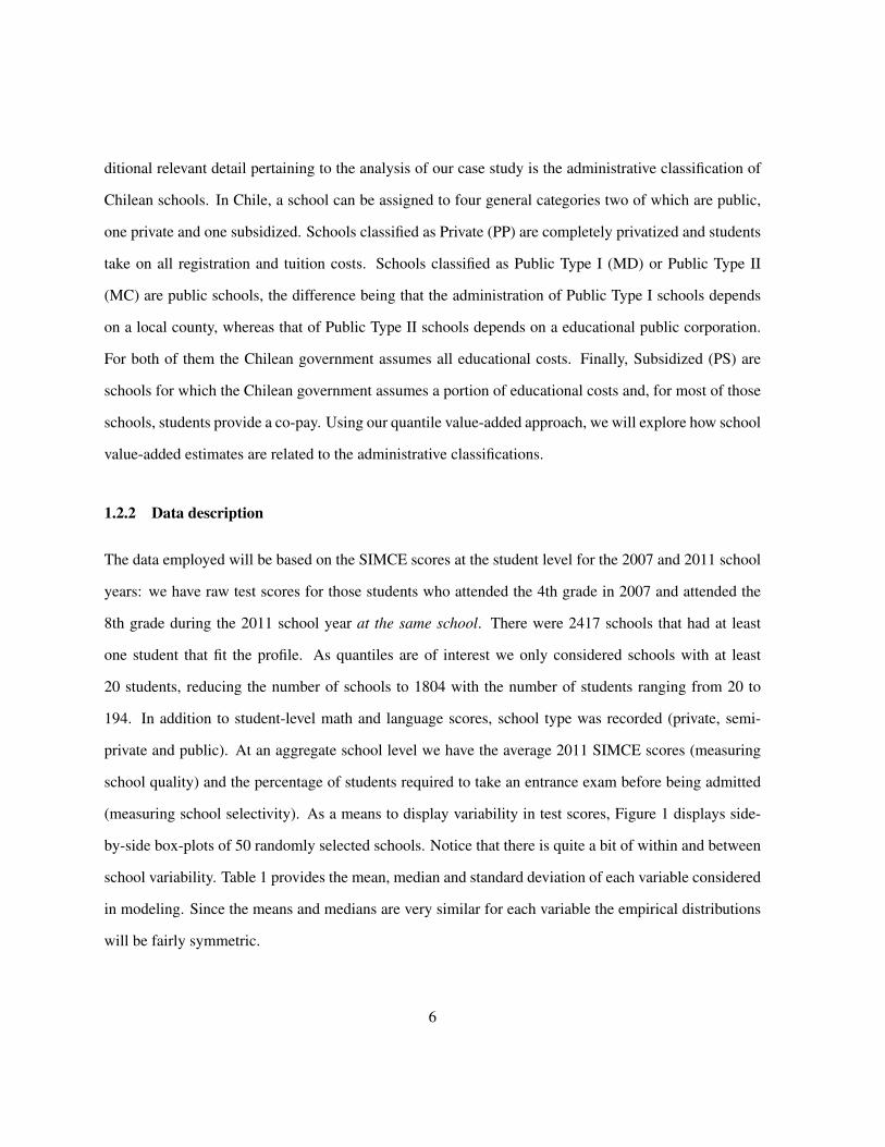
1.2.2 Data description
The data employed will be based on the SIMCE scores at the student level for the 2007 and 2011 school
years: we have raw test scores for those students who attended the 4th grade in 2007 and attended the
8th grade during the 2011 school year at the same school. There were 2417 schools that had at least
one student that fit the profile. As quantiles are of interest we only considered schools with at least
20 students, reducing the number of schools to 1804 with the number of students ranging from 20 to
194. In addition to student-level math and language scores, school type was recorded (private, semi-
private and public). At an aggregate school level we have the average 2011 SIMCE scores (measuring
school quality) and the percentage of students required to take an entrance exam before being admitted
(measuring school selectivity). As a means to display variability in test scores, Figure 1 displays side-
by-side box-plots of 50 randomly selected schools. Notice that there is quite a bit of within and between
school variability. Table 1 provides the mean, median and standard deviation of each variable considered
in modeling. Since the means and medians are very similar for each variable the empirical distributions
will be fairly symmetric.
6

Table 1: The mean, median and standard deviation of variables that were included in modeling.
Variable Mean Median Std Dev
2011 SIMCE Math Score 267.657 267.055 49.5082007 SIMCE Math Score 260.664 263.200 52.858Average 2011 SIMCE Math Score 260.664 259.610 29.233% Students that took entrance exam 0.434 0.328 0.391
●
●
●
●
●
●●
●
●●
●
●
●
●
●
●
●
●
●
●
●
●
●
●
●
●
●
150
200
250
300
350
400
School
SIM
CE
Mat
h 20
11 S
core
Figure 1: Boxplots of individual 2011 SIMCE math scores for 50 randomly selected schools
7

1.3 Organization of the paper
The rest of the paper is organized as follows. In Section 2 we introduce a model free definition of
value-added and then extend it to the quantile value-added case. The model that provides (quantile)
value-added estimates is also introduced in this section. In Section 3 methods used to estimate quantile
value-added are developed. Section 4 contains results from the Chilean education case study illustrating
the benefits of the proposed approach. The paper finalizes in section 5 with conclusions and discussion.
2 Definition of Quantile Value-Added
It should be clear at this point that school effect and value-added are two different concepts the former
being used to obtain the latter. From a modeling point of view, both concepts are typically defined in the
context of a hierarchical linear model (HLM) (Aitkin and Longford 1986; McPherson 1992; Raudenbush
and Willms 1995; Goldstein 1997; Tekwe et al. 2004; Raudenbush 2004). However, one may wonder
if these concepts can be defined independently of a specific structural model –that is, a model that at-
tributes the stochastic generation of the observations to an underlying structure representing a (part of a)
substantive theory? (for details on structural models, see Mouchart et al. 2010; Wunsch et al. 2014, and
the references therein). Manzi et al. (2014) addressed this question, and proposed a model-free definition
of school effect and value-added. The advantages of such a definition are twofold: on the one hand, we
distinguish between the structural definition of a concept and its statistical estimation; on the other hand,
the assumptions necessary to define those concepts become explicit.
Taking insight from the structure underlying HLM models, Manzi et al. (2014) provide one possible
model-free definition of school effect and value-added. To make ideas concrete we introduce the basic
notation that will be used through out. Let Yij be the test score of student j belonging to school i
for i = 1, · · · ,m and j = 1, · · · , ni; let Xij be a corresponding vector of p covariates which can
contain both school and student-specific variables and let αi denote school i’s latent variable (which also
8

represents school effect).
2.1 Model-free definition of school effect
A school effect is characterized by the amount of heterogeneity in Yij explained by a school after having
taken into account the heterogeneity of Yij explained by the Xij’s. The school effect αj is accordingly
defined by the following two structural conditions:
1. For each school i, {Yij : j = 1, . . . , ni} are mutually independent conditionally on (Xi, αi),
whereXi = (Xi1, . . . ,Xini).
2. For each school i and for each student j = 1, . . . , ni, the conditional distribution of (Yij |Xi, αi)
only depends on (Xij , αi).
Notice that condition (1) and (2) are an example of the Axiom of Local Independence introduced by
Lazarsfeld (1950) and commonly used in psychometrics, statistics and educational measurement to de-
fine latent variables and/or random effects. Using the standard properties of condicional expectation the
following is easily shown
cov(Yij , Yij′ |Xi) = cov[E(Yij |Xij , αi), E(Yij′ |Xij′ , αi) |Xi].
This equality shows that the school effect αj induces heterogeneity on the Yij’s through the conditional
expectation (or regression) E(Yij |Xij , αj), which is not necessarily linear, but an arbitrary function of
(Xij , αj).
2.2 Model-free definition of value-added
The covariance result from the previous section leads one to define school value-added in terms of the
regression E(Yij | αj ,Xij). However, the reasoning behind the theoretical concept of value-added
9

discussed in the introduction should also be considered. Mainly, to identify which part of Yij can be
attributed to the school. In order to do so, assuming that the random variables are square-integrable, the
score Yij can be decomposed in three orthogonal (or uncorrelated) components:
Yij = E(Yij |Xij) + {E(Yij | αi,Xij)− E(Yij |Xij)}+ {Yij − E(Yij | αi,Xij)} . (2.1)
The first component on the right hand side of (2.1) captures the covariate’sXij contribution on the score
Yij . The second component captures the school effect’s (αi) contribution on Yij after taking into account
the contribution of the covariates Xij . The third component corresponds to the idiosyncratic error, that
is, the “part” of Yij which is not statistically explained by the school effect αi, nor by the covariatesXij .
From decomposition (2.1), it is clear that the second component is school dependent and as a result,
may be considered to be under its control. This leads to define the school i’s value-added in terms of an
average of the second component, namely
VAi =1
ni
ni∑j=1
E(Yij | αi,Xij)−1
ni
ni∑j=1
E(Yij |Xij). (2.2)
The first term represents an average of the expected score in a specific school, after taking into account
the covariates. The second term corresponds to an average of the expected score in the “average” or “ref-
erence” school, after controlling for the covariates. This last interpretation rests on the general property
E(Yij |Xij) = E[E(Yij |Xij , αi) |Xij ], which is obtained after integrating αi.
To estimate school value-added, a structural model describing the generation of (Yij ,Xij , αi) needs to
be specified. For example, if the regression E(Yij | Xij , αi) is assumed to be linear and the covariates
Xij are independent of the school effect αi, that is,
(i) (Yij |Xi, αi) ∼ N (X ′ijβ + αi, σ2), (ii) (αi |Xi) ∼ N (0, σ2α), (2.3)
and the distribution of the covariatesXij is left unspecified, then Definition (2.2) implies that the school
10
value-added is equivalent to the school effect (note that condition (2.3.ii) implies that cov(αi,Xi) =
cov(E(αi | Xi), αi) = 0). However, if cov(αi,Xi) 6= 0, Definition (2.2) implies that the value-added
is equal to the school effect corrected by an additive term; for details, see Manzi et al. (2014) and Bates
et al. (2014).
2.3 Consequences of the model-free definition of school effect and value-added
The model-free definitions of school effect and value-added carry with them some consequences regard-
ing the meaning of a value-added analysis. First, because the school effect induces correlation on the
test scores, the schools in a value-added analysis are characterized by a common feature. Namely, each
school is an entity that produces heterogeneity in the students’ achievements as measured by the test
scores Yij . Such heterogeneity remains in the students’ achievements after controlling for observable
covariates at both student and school level.
Second, Definition (2.2) provides a characterization of the “average” or “reference’ school which is
completely determined by the vector of covariates Xi. It is well known in the school effectiveness lit-
erature that a value-added analysis is relative to an “average” school. Consequently, if the reference
changes, the value-added indicators might change, sometimes drastically. Definition (2.2) not only ex-
plains why this happens, but also shows in what sense a value-added analysis is covariate-dependent: if
the covariates change, not only does the “average” school change, but also the meaning of school ef-
fectiveness. Thus, covariates need to be selected based on the policies that motivated the value-added
analysis. For instance, Raudenbush and Willms (1995) and Raudenbush (2004) (see also Timmermans
et al. 2011; Milla et al. 2014) consider lagged score as the only covariate. In this case, value-added
measures the school’s effectiveness in educating students after controlling for their initial lagged scores
and school effectiveness is only related to students. In light of this, value-added results from this model
should only be used when pursuing policies based on identifying schools that are effective in developing
student schooling. However, if we consider both the lagged score and a compositional effect (defined,
11

for each school, as the average of the lagged score) as covariates, then we are not only controlling for the
initial level of each student, but also for the student cohort level. This type of value-added model will
measure the effectiveness of a school to educate students taking into account not only their individual
initial achievement level, but also their cohort level. Consequently, the usability of this type of model in
terms of policy is related to possible difference between pedagogical methods. Qualitative observations
should be made to understand such differences (Hofman et al. 2015). These considerations lead one to
conclude that school effectiveness is not a universal concept, but a contextual idiosyncratic one. The
context is characterized by the covariates introduced in the model. Their selection as well as their mean-
ing is highly dependent on the policy context under which a value-added analysis is required, as well as
on the social context in which an educational system is organized.
Third, as mentioned previously, estimating value-added via Definition (2.2) requires the specification
of a structural model that describes the generation of (Yij ,Xij , αi). The assumptions and hypotheses
underlying the structural model should be justified with respect to the specific context in which the value-
added analysis is being carried out.
Finally, note that Definition (2.2) is based on students’ “average” performance in a given school. A
natural generalization would be to consider percentiles of (Yij | αi,Xij) and (Yij |Xij) which we now
detail.
2.4 Definition of Quantile Value-Added
Let QY (τ |X) = inf{y : FY (y|X) ≥ τ} denote the τ th quantile of Y given covariate X . Put another
way, QY (τ |X) is the value such that τ = Pr(Y < QY (τ |X)) = FY (QY (τ |X)) =∫ QY (τ |X)−∞ fY (y)dy
where FY (·) and fY (·) denote the cumulative distribution and density function of Y respectively. With
this notation in mind, a natural extension of (2.2) is
qVAi =1
ni
ni∑j=1
QYij |αi(τ |Xij)−1
ni
ni∑j=1
QYij (τ |Xij). (2.4)
12

As remarked above, in the absence of endogeneity (i.e., when cov(αi,Xi) = 0), HLM (2.3) produces
an estimate of (2.2) and we will show in next section that a linear quantile mixed model framework
produces an estimate of (2.4). Further, since we adopt a Bayesian approach inference associated with
qVA is readily available. Lastly, similar to how the median is robust to the presence of outliers relative
to the mean, a VA estimate at the 50th percentile using the method we will propose will be more robust
to the presence of outliers than (2.2) and other typical mean type value-added estimators available in the
literature.
2.5 Linear Quantile Mixed Models
To begin, we briefly review basic quantile regression which now has a substantial literature (Koenker
2005) and then consider quantile mixed models and qVA estimation.
Analogous to how least squares regression is the solution to minimizing squared error loss, classical
quantile regression is the solution to the following check loss function minimization problem for a pre-
specified quantile τ
arg minβ(τ)
n∑i=1
ρτ (Yi −X ′iβ(τ)) (2.5)
where ρτ (u) = u(τ − I[u < 0]). An alternative criterion that is analogous to specifying Yi = Xiβ + εi
with E(εi) = 0 in linear models is, for some pre-specified quantile τ ∈ (0, 1), proposing the following
model
Yi = X ′iβ(τ) + ε
(τ)i with Qεi(τ) = 0. (2.6)
A result of (2.6) is that QYi(τ |Xi) = X ′iβ(τ), which is related to how linear mean models produce
E(Yi) = X ′iβ. Additionally, it has been shown that the value of β(τ) that minimizes (2.5) is the same
value that maximizes (2.6) under an asymmetric Laplace distribution (ALD) ε(τ)i whose τ th quantile is 0.
13

We will use the notation ε ∼ ALD(µ, σ, τ) to denote that ε follows a ALD distribution with parameters
µ, σ, and τ . Under this distribution ε has the following density
p(ε; τ, µ, σ) =1
στ(1− τ) exp
{−ε− µ
σ(τ − I[ε− µ < 0])
}. (2.7)
Since∫ µ−∞ p(ε; τ, µ, σ)dε = τ , we have µ = 0 =⇒ Qεi(τ) = 0 so that in what follows we set µ = 0.
Quantile based methods dedicated to longitudinal or hierarchical data have also been addressed in the
literature (see, for example, Geraci and Bottai 2013; Reich et al. 2010; Geraci and Bottai 2007). Using
this approach in education studies is not unprecedented. Levin (2001) used quantile regression to argue
that there is evidence of positive peer effects in the lower percentiles of the achievement distribution, and
Miranda et al. (2009) use quantile regression to explore how social and environmental factors influence
the tails of end-of-grade test scores in the state of North Carolina. Additionally, quantile regression is
employed in student growth percentile (SGP) models (Betebenner 2008, Lockwood and Castellano 2015)
andGuarino et al. (2015) conducts a simulation study that compares teacher assessment available from
SGP models to that from three types of mean-based value-added estimates.
Similar to linear mixed models the straightforward extension is to add a latent school effect so that
Yij = X ′ijβ(τ) + α
(τ)i + ε
(τ)ij . (2.8)
Note that α is a function of τ in addition to β and ε(τ)ij ∼ ALD(0, σ, τ) independent of α(τ)
i ∼
N(µα, σ2α). From properties of the ALD QYij |αi(τ |Xij) = X ′ijβ
(τ) + α(τ)i . µα implicitly depends
on τ and represents a global intercept with α(τ)i representing local (school) deviations. It is common
in mixed model applications to set µα = 0, but we elect to proceed with a more general mixed model
formulation as there is no reason to believe a prior that E(α(τ)i ) = 0.
A key reason we introduce the model based quantile linear mixed model in (2.8) with error term (2.7) is
that a valid likelihood is produced making a Bayesian approach viable. Consequently, prior distributions
14

for β(τ), µα, σ2α, and σ need to be specified. We employ a conjugate prior for regression coefficients
and assume that β(τ) ∼ N(b0,B0). Additionally, we employ µα ∼ N(0, s2µ), σ2α ∼ IG(aα, bα) and
σ ∼ IG(aσ, bσ) with IG(a, b) denoting an inverse gamma distribution with mean b/(a− 1).
We briefly mention here that unless linear constraints are added to the errors of (2.6) and (2.8), the
quantile curves could possibly cross. This is particularly true when tail quantiles are desired and little
data are available. There has been work dedicated to avoiding this (see He 1997 for fixed effects models
and Lum and Gelfand 2012 for mixed models). However, such methods drastically complicate the anal-
ysis and therefore we opt to employ the mixed quantile model just described. Even though simplicity
motivated the decision, quantile curve crossing is uncommon when a large number of observations are
available, which is the case in the application we consider.
Finally, we studied the identifiability of the proposed model based on the first and second moment
of the three-parameter asymmetric Laplace distribution (see Yu and Zhang 2005). We found that the
model is indeed identifiable under the following conditions: τ must be pre-specified (i.e., it cannot be
an unknown), αi and εij must be iid, σ > 0, and X must not contain a vector of ones representing an
intercept (if not, µα is unidentified). These conditions are all easily satisfied within the framework in
which the model was constructed.
3 Quantile Value-Added Estimation
We now proceed to detail how (2.4) will be estimated using (2.8). To estimate (2.4) the τ th quantile of
(Yij | Xij , αi) and (Yij | Xij) needs to be computed. Through properties of the ALD, the quantile
conditional on αi is readily available with QYij |αi(τ |Xij) = X ′ijβ(τ) + α
(τ)i . Calculating QYij (τ |Xij)
is much more difficult. A few researchers have discussed estimating the marginal quantile. For example,
Reich et al. (2010) specify a completely new model so that the marginal quantile corresponds toX ′ijβ(τ).
Also, Geraci and Bottai (2013) mention marginal quantile effect estimates but focus attention on the
difficulty of their interpretation. That said, none of the methods in the literature propose simultaneously
15

estimating both quantiles by way of a unified modeling approach.
The main difficulty in estimatingQYij (τ |Xij) coherently from (2.8) is calculating the marginal density
of Yij . Since ε(τ)ij is no longer Gaussian marginalizing (2.8) over αi is not straightforward. However,
notice that Yij is a sum of two independent random variables ε(τ)ij and Z(τ)ij = X ′ijβ + α
(τ)i (one being
ALD and the other Gaussian). Therefore, we can use convolution techniques to derive the marginal
density of Yij . (Geraci and Bottai (2013) also address deriving the marginal density of Yij but using a
different approach.) The convolution of Z(τ)ij and ε(τ)ij turns out to be (see details in the appendix and for
notational convenience i, j subscripts and (τ) superscript were dropped)
fY (y) =
∫fZ(y − ω)fε(ω)dω
=1
στ(τ − 1)φ(y;X ′β + µα, σ
2α)
×
[φ−1
(y;X ′β + µα +
σ2ασ
(τ − 1), σ2α
)Φ
(−X ′β + µα − σ2
ασ (τ − 1)
σα
)+
φ−1(y;X ′β + µα +
σ2αστ, σ2α
)Φ
(X ′β + µα − σ2
ασ τ
σα
)], (3.1)
where φ(·;m, s2) denotes a Gaussian density with mean m and variance s2 and Φ(·) denotes a standard
Gaussian cumulative distribution function. Calculating QYij (τ |Xij) can now be carried out employing
(3.1). Even though the marginal density of Yij is somewhat complex, using it to estimate QYij (τ |Xij)
is conceptually straight forward. Numerically it would be possible to evaluate (3.1) for a sequence of
possible Y values and then simply select the Y value that corresponds to the empirical τ th quantile.
This is facilitated through the usual computational algorithms employed in a Bayesian analysis which
we detail in the next section.
16

3.1 Computation
Since we’ve adopted a Bayesian approach inference is based on the joint posterior distribution
p(β(τ), σ, µα, σ2α,α
(τ)|Y ,X). (3.2)
As this distribution is analytically intractable, we resort to using MCMC techniques to sample from it.
To facilitate sampling, as detailed in Lum and Gelfand (2012) and Yue and Rue (2011) we characterize
the ε ∼ ALD(0, σ, τ) with the following scale mixture of normals
ε =
√2ξσ
τ(1− τ)ζ +
1− 2τ
τ(1− τ)ξ, (3.3)
where of ζ ∼ N(0, 1) and ξ ∼ Exp(σ) with E(ξ) = 1/σ. Introducing auxiliary variables ζ and ξ facil-
itates computation as the augmented likelihood (by ζ) becomes Gaussian and the augmented parameter
vector (β, σ, µα, σ2α,α, ξ) produces recognizable full conditionals making it possible to employ a Gibbs
sampler (full conditionals are provided in the Appendix). Therefore, draws from (3.2) can be collected
by cycling through the full conditionals on an individual basis.
3.2 Estimation and Inference
Since qVA is a function of (β(τ), σ, µα), once B MCMC iterates of p(β(τ), σ, µα,α(τ)|Y ,X) are col-
lected they can be used to produce MCMC draws from p(qVAi|Y ,X) (the posterior distribution of the
ith schools qVA) from which all estimation and inference is derived. For example, a reasonable estimator
of the ith schools qVA is
qVAi = E[qVAi|Y ,X] =1
ni
ni∑j=1
E[QYij |αi(τ |Xij)|Y ] +1
ni
ni∑j=1
E[QYij (τ |Xij)|Y ].
17

Now using the B MCMC iterates collected from p(β(τ), σ, µα,α(τ)|Y ,X) a Monte Carlo estimate of
E[QYij |αi(τ |Xij)|Y ] is simply
QYij |αi(τ |Xij) =1
B
B∑b=1
X ′ijβ(τ)(b) + α
(τ)(b) (3.4)
where subscript (b) indexes the bth MCMC iterate. Since fY (y) is a function of (β, σ, µα, σ2α,α),
the MCMC iterates can also be employed to estimate QYij (τ |Xij) as Monte Carlo simulation (within
the MCMC algorithm) can be used to produce draws from p(QYij (τ |Xij)|Y ). This is done by dis-
cretizing a suitable interval of Y into M plausible values and for each evaluating 3.1 at each of the
b MCMC iterates. The τ th empirical quantile of the M density values would represent the bth draw
from p(QYij (τ |Xij)|Y ). Letting Q(b)Yij
(τ |Xij) denote the bth MCMC draw, a Monte Carlo estimate of
E[QYij (τ |Xij)|Y ] is
QYij (τ |Xij) =1
B
B∑b=1
Q(b)Yij
(τ |Xij).
Finally, a Monte Carlo estimate of qVA is
qVAi =1
ni
ni∑j=1
QYij |αi(τ |Xij)−1
ni
ni∑j=1
QYij (τ |Xij). (3.5)
Under the Bayesian paradigm, intervals associated with qVA are also very easily computed once B
MCMC iterates of p(β(τ), σ, µα,α(τ)|Y ,X) have been collected. Among the B iterates, one simply
needs to find values L and U such that Pr(L ≤ qVA ≤ U |Y ,X) = 1 − c for some pre-specified
c ∈ (0, 1). In the results section we find L and U that are associated with the 95% Highest Posterior
Density (HPD) intervals (Gelman et al. 2013).
Although it may be obvious, it is worth noting that the computational procedure just described for car-
rying out estimation and inference must be run for each student and therefore becomes computationally
18

expensive as the number of students grow.
4 Application: Chilean SIMCE Test Data
As discussed in the introduction, the role of the Chilean National Agency of Quality of Education is to
evaluate students’ achievement as well as the performance of schools according to national standards.
This information is used to produce a classification of schools. Interestingly the SAC law contemplates
the possibility of performing such a classification using value-added models. It should be mention, how-
ever, that the Chilean National Agency of Quality of Education has ruled it out at this time. Therefore in
the light of wider debates regarding the meaning and measurement of school effectiveness it is relevant to
discuss the information produced by value-added methodologies that schools potentially can obtain. The
objective of this section is to illustrate information that is available from quantile value-added indicators
using the Chilean data set described in Section 1.2.2.
4.1 Preliminary Remarks
In order to build some intuition regarding how qVA is computed and the information it provides we
first consider a regression model with only one subject specific covariate (2007 SIMCE Math score).
Subsequently we consider a regression model with three covariates that are known to be exogenous two
of which are school specific (2007 SIMCE Math Score averaged over school, and percent of students
who took and entrance exam prior to be admitted to school) and one which is student-specific (individual
2007 SIMCE Math Score). As mentioned in the introduction, decisions regarding covariate inclusion
can greatly impact not only value-added estimates, but also their substantive meaning; these issues will
be illustrated by discussing the qVA from each model.
The dependent variable Yij corresponds to the 2011 SIMCE math score, whereas the prior attainment
score X1ij corresponds to the 2007 SIMCE math score. It is important to note that the 2007 SIMCE
test was administered at the end of the first half (fourth grade) of primary education, whereas the 2011
19

SIMCE test is administered at the end of the second half (eighth grade) of primary education. In the
Chilean educational system, there exists a difference between the first half and the second half: during the
first half of primary education, Mathematics, Language, Sciences and Arts are taught by one teacher only
(a generalist teacher). During the second half of primary education, those topics are taught by subject-
specific teachers. Therefore, the value-added analysis reported below aims to estimate a school’s ability
to effectively carry out the second half of primary education after controlling by the scores obtained at
the end of the first half of primary education. The difference between the first half and the second half of
primary education justifies the exogeneity of the prior attainment score X1ij . In fact, we argue that this
difference represents a different school organization at both administrative and educational level.
Details regarding computation associated with fitting the two models are the same so we detail them
here. Both models were fit using methods described in Section 3. To improve mixing, we considered
Yij − Y and Xij − X where Y =∑
ij Yij/N and X =∑
ij Xij/N with N =∑m
i=1 ni (this doesn’t
influence qVA estimates as differences between marginal and conditional quantiles remain unchanged.)
For each τ considered, qVA was estimated using 1000 MCMC iterates after discarding the first 1000
as burn-in. Convergence was monitored graphically by examining MCMC iterate history plots which
displayed fair mixing and fast convergence. We selected prior parameters values that would provide
“weakly informative” priors (Gelman et al. 2013) and resulted in the following b0 = 0,B0 = s2βI , with
s2β = 1002, aσ = aα = bσ = bα = 1, and s2µ = 1002.
4.2 Model with One Covariate
Recall X1ij denotes the 2007 SIMCE math score of ith student from the jth school and Yij denotes the
2011 SIMCE math score for the same student (we emphasize again that only students who attend the
same school in 2007 and 2011 are considered). To estimate qVA we fit the following model
Yij = X1ijβ(τ)1 + α
(τ)i + ε
(τ)ij i = 1, . . . ,m, j = 1, . . . , ni (4.6)
20

0.54 0.56 0.58 0.60 0.62 0.64
050
100
150
200
β(τ)
Den
sity
τ = 0.05τ = 0.1τ = 0.25τ = 0.5
τ = 0.75τ = 0.9τ = 0.95
●
●
●
●
●
●
●
0.54
0.56
0.58
0.60
0.62
0.64
β(τ)
τ0.05 0.25 0.5 0.75 0.9
Figure 2: The left plot displays the marginal posterior distributions of β(τ). The right plot displays theposterior means and 95% credible intervals of β(τ) as a function of τ
for τ = 0.05, 0.1, 0.25, 0.5, 0.75, 0.9, 0.95.
To illustrate that the relationship between 2007 and 2011 SIMCE math scores depends on τ we provide
Figure 2. It appears that moving from τ = 0.05 to τ = 0.1 produces a slight increase in β(τ) and then
a gradual decreases as τ moves from 0.1 to 0.95. The decrease in β(τ) as τ increases is to be expected
in the current setting since improving upon a high test score is more difficult than improving upon a low
one. Table 2 provides the posterior means and standard deviations of β1 for each τ . The same trends
seen in Figure 2 are present.
4.2.1 Comparing the qVA for τ = 0.5 with standard mean value-added estimates
Before highlighting the information that quantile value-added provides over mean value-added, we show
that the qVA estimate for τ = 0.5 is very similar to the value-added estimate from two very common
mean-based estimators. Both mean-based estimators are derived from the HLM found in equation (2.3).
The first method employs maximum likelihood estimation and therefore the value-added estimates cor-
21

1 2 3 4 5 6
−20
020
40
school
Val
ue A
dded
Est
imat
e
●
●
●
●
●
●
●
●
●
●
●
●
●
●
●
●
●
●
LMMBHLMMqVA0.5
Figure 3: Three value-added estimates with 95% intervals associated with six schools and model withone covariate. The left and middle intervals (dashed and dotted vertical line’s) are based on a HLM withthe left corresponding to maximum likelihood estimation and the middle a Bayesian model. The intervalson the right (dash-dot vertical line) correspond to qVA for τ = 0.5.
22

Table 2: The posterior expectations and standard deviations associated with the coefficients from themodel with one covariate (β1 - previous attainment score) and three covariates (β1 - previous attainmentscore, β2 - school average test score, β3 - % of students that took entrance exam)
One Covariate Model Three Covariate Model
τ E(β1) sd(β1) E(β1) sd(β1) E(β2) sd(β2) E(β3) sd(β3)
0.05 0.633 0.003 0.625 0.104 13.682 0.003 0.018 1.4960.10 0.641 0.003 0.632 0.141 13.354 0.003 0.017 1.1240.25 0.635 0.003 0.624 0.137 14.497 0.002 0.017 1.2680.50 0.619 0.003 0.608 0.161 13.623 0.003 0.016 1.0070.75 0.587 0.003 0.577 0.182 14.314 0.002 0.011 0.9030.90 0.561 0.002 0.552 0.211 14.288 0.002 0.020 1.1280.95 0.548 0.002 0.541 0.222 14.110 0.002 0.014 0.783
respond to the so called best linear unbiased predictors (BLUP)’s. BLUP uncertainty and inference are
derived through the asymptotic results that accompany maximum likelihood estimation and are carried
out using the lmer function of the statistical software R. The second method of estimating value-added
is based on a the following Bayesian model:
(Yij |Xij ,β, αi, σ2i ) ∼ N (Xijβ + αi, σ
2i )
αi ∼ N(ma, s2a)
β ∼ Np(mb, s2bI)
σ2i ∼ IG(as, bs)
Estimation and inference associated with the value-added from this model is based on the posterior
distribution of (β,α,σ2). Using MCMC methods, draws from this distribution were collected and
employed to estimate value-added and construct 95% intervals. We will refer to the maximum likelihood
estimate as LMM and the Bayesian estimate as BLMM. Figure 3 provides the value-added estimates and
95% intervals from LMM and BLMM along with a qVA estimate and interval for τ = 0.5 associated
23

with six schools. The six schools were selected based on their ability to highlight qVA advantages and
will be referenced through out the remainder of the paper. Notice that for these six schools the three
procedures produce very similar value-added estimates. In fact, the correlation coefficient between the
LMM value-added and qVA for all schools is approximately 0.97 while that for BLMM and qVA is
approximately 0.98.
4.2.2 Illustrating the meaning of the qVA
In order to build intuition regarding the meaning of qVA, we provide Figure 4 which contains results
from two schools for τ = 0.05, 0.25, 0.75, and 0.95. The schools were selected as they clearly illus-
trate value-added’s dependance on τ . In the figures the solid black line represents QYij (τ |Xij), while
the dashed and dotted gray lines represent QYij |αi(τ |Xij) for each school respectively. The circled
cross points highlighted on each respective schools quantile regression line (blue and red lines) represent
1ni
∑nij=1 QYij |αi(τ |Xij), while the asterisk points on the solid black line represent 1
ni
∑nij=1 QYij (τ |Xij)
for each school. The vertical distance between these two points represents each school’s qVA estimate.
Thus, for τ = 0.05 the dashed line school has a positive qVA while that of the dotted lined school is
negative. For τ = 0.25 and τ = 0.75 both schools have a negative qVA but the rankings invert moving
from from τ = 0.25 to τ = 0.75. Finally, for τ = 0.95 the dotted lined school now has a highly negative
qVA while the dashed lined school’s qVA is positive.
4.2.3 How informative are the qVA scores?
Now we consider value-added as a function of τ . Figure 5 presents qVA for the same 6 schools shown in
Figure 3. Notice the large variability of qVA not only between schools but with in school. Two schools
appear to have a positive qVA for each of the 7 percentiles considered meaning that the cloud of points
associated with those two schools is always concentrated above the majority of schools. Those schools
whose value-added moves from negative to positive typically have a cloud of points that is much more
24
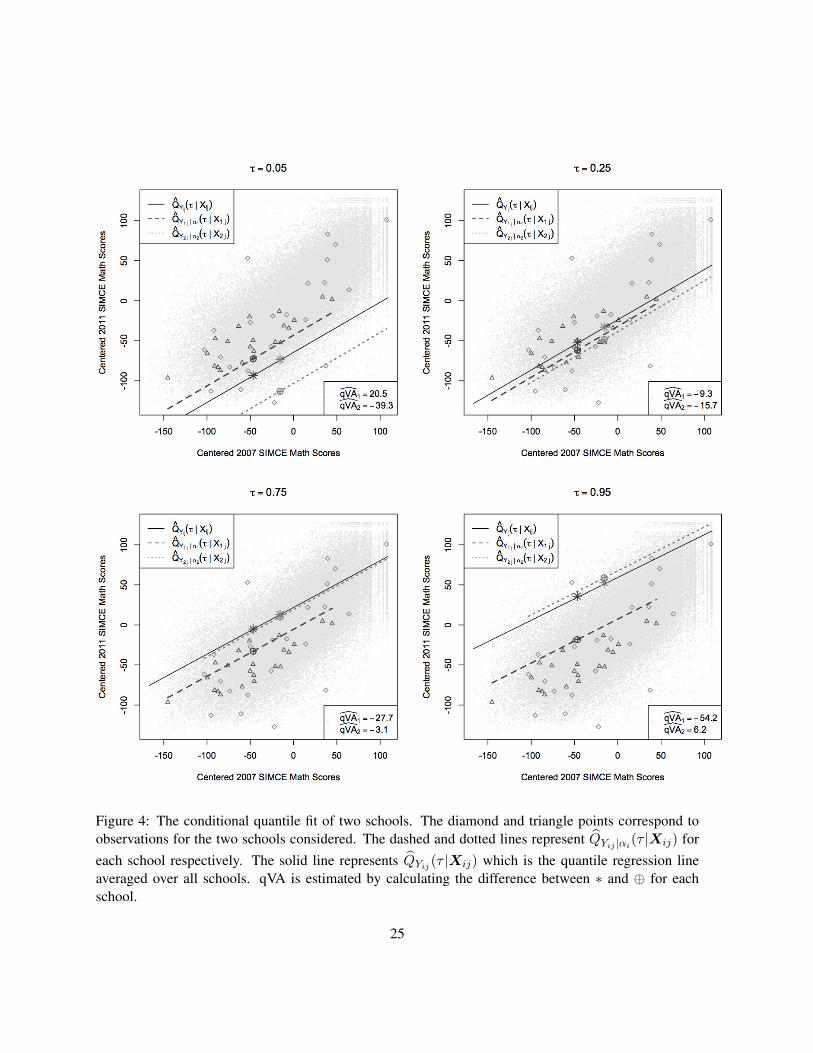
Figure 4: The conditional quantile fit of two schools. The diamond and triangle points correspond toobservations for the two schools considered. The dashed and dotted lines represent QYij |αi(τ |Xij) foreach school respectively. The solid line represents QYij (τ |Xij) which is the quantile regression lineaveraged over all schools. qVA is estimated by calculating the difference between ∗ and ⊕ for eachschool.
25

τ
Qua
ntile
Val
ue A
dded
0.05 0.1 0.25 0.5 0.75 0.9 0.95
−60
−40
−20
020
4060
●
●
●
●
●
●
●
●
school 1school 2
school 3school 4
school 5school 6
Figure 5: qVA estimate from model that includes one covariate for six schools that were selected tohighlight information that qVA provides.
26

variable and have students with very high and low scores. It is interesting to note that the lines plotted in
Figure 5 often cross and therefore, rankings of schools based on value-added depends a great deal on the
test-score distribution percentile.
τ
Qua
ntile
Val
ue A
dded
0.05 0.1 0.25 0.5 0.75 0.9 0.95
−60
−40
−20
020
4060
●
●
●
●
●●
●
●
●
●
●
●
●
●
●
●
●
●
●
●
●
●
●
● ●
●
●
●
●
●
●
●
●
●
●
●
●
●
●
●
● ●
Figure 6: 95% Bayesian intervals corresponding to same six schools as in Figure 5.
Figure 6 presents 95% Bayesian highest posterior density intervals that correspond to the six previously
mentioned schools. There is a fair amount of variability at each quantile. That said, two schools are su-
perior in terms of value-added for all quantiles besides the 95th. Notice further that the school associated
with the dotted line has the lowest value-added for scores in the 5th quantile, but steadily improves as
the test score quantiles increase and eventually being centrally ranked. The schools associated with the
solid and dashed lines produce value-added that is very similar except for the 90th and 95th percentile.
Generally speaking, Figures 5 and 6 clearly show that focusing only on mean type value-added estimates
27

(corresponding to τ = 0.5) is insufficient in characterizing a schools effectiveness.
4.2.4 Relating the qVA to administrative characteristic of schools
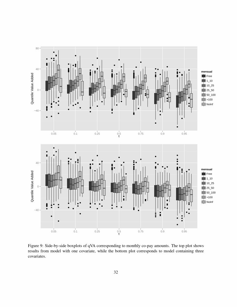
Next we consider the effect that school type has on quantile value-added. The top plot of Figure 7
provides side-by-side box plots of qVA estimates for all schools grouped according to school type. From
this plot it appears that value-added associated with PP schools is consistently higher than other types
of schools regardless of τ . The two public school types produce similar value-added for each τ and the
subsidized schools seem to provide some added value relative to the public schools. To further investigate
this phenomena we partition schools according to the amount of co-pay (or total for PP schools) that is
charged. These results can be seen in Figure 9, first panel. From the figure it can be seen that for each
quantile τ , school effectiveness increases in conjunction with co-payment. Notice that there appears to
be an overall negative trend in Figures 7 and 9. This confirms the intuition that it is “easier” for a school
to demonstrate effectiveness with students who have a low prior attainment score relative to those that
have high prior attainment scores.
Finally, in context of the Chilean education system (see Section 1.2), the value-added based on model
(4.6) measures the effectiveness of a school to educate students after controlling for their initial SIMCE
scores. That is, the effectiveness of a school is only related to the students. Therefore, one way qVA
might be useful in guiding policy decisions is that it identifies effective schools regarding a schooling
period characterized by multiple disciplines and teachers because qVA shows which schools are more
effective with students at different initial quantile levels (a Type A indicator according to Raudenbush
and Willms (1995)’s terminology).
4.3 Model with Three Covariates
We now consider Xij as a vector of three covariates. We retain Xij1 = individual student 2007 SIMCE
math score and now add Xij2 = percentage of students required to take entrance exams before being
28

●
●
●
●
●
●
●
●●●
●●
●
●
●
●
●
●
●
●
●
●
●
●
●
●●
●●
●
●
●
●
●●
●
●
●
●●●
●
●
●
●
●
●
●
●
●●●
●
●
●
●●
●●
●●
●
●●
●●●
●●
●
●●
●
●
●●●
●
●
●●
●
●
●●●●●
●
●
●
●●
●●
●●
●
●
●
●●
●●
●
●●
●
●●
●
●
● ●
●●●
●
●●
●
●
●
●
●●●
●
●●
●
●
●●●●
●
●
●●
●
●
●
●●
●
●
●
●●●
●
●
●
●
●
●
●
●●
●
●●
●
●
● ●●
−40
0
40
80
0.05 0.1 0.25 0.5 0.75 0.9 0.95τ
Qua
ntile
Val
ue A
dded
school_type
MC
MD
PP
PS
●
●
●●
●
●●
●●
●
●
●
●●
●
●
●
●
●
●
●
●
●
●●●●
●
●
●●●
●
●
●
●
●
●●
●
●
●
●
●
●
●●
●
●
●
●
●
●●
●
●●
●
●
●
●
●
●
●
●
●
●
●
●
●●●
●
●●
●
●
●
●
●●
●
● ●
●●●
●●
●
●
●●
●
●
●●
●
●
●
●
●
●
●●
●
●
●
●
●
●
●
●
●
●●
●
●
●
●
●●
●
●
●
●●
●●●
●
●
●
●
●
●
●
●
●
●●
●●●
●
●
●●
●
●
●
●
●
●
●●
●
●●●
●
●
●
●●
●
●●
●
●
●●
●
●
●
●
●
●
●
●
−40
0
40
0.05 0.1 0.25 0.5 0.75 0.9 0.95τ
Qua
ntile
Val
ue A
dded
school_type
MC
MD
PP
PS
Figure 7: Side-by-side boxplots of qVA corresponding to the four school types in the Chilean educationsystem. PP represents private schools, PS public schools with co-pay and MD, MC are two differenttypes of public schools. The top plot shows results from model with one covariate, while the bottomplot corresponds to model containing three covariates. For each τ , the first box-plot (moving from left toright) corresponds to MC, the second MD, third PP, and fourth PS.
29

admitted and Xij3 = school average 2007 SIMCE math score. For the same τs considered in Section
4.2, we fit the following model
Yij = Xij1β(τ)1 +Xij2β
(τ)2 +Xij3β
(τ)3 + α
(τ)i + ε
(τ)ij i = 1, . . . ,m, j = 1, . . . , ni. (4.7)
Figure 8 provides a plot of qVA as a function of τ for the same six schools as those found in Figure
5. Generally speaking one effect of incorporating three covariates when estimating qVA is that between
school variability associated with qVA has decreased. This is to be expected as the added covariates
explain more variability between schools. Additionally, adding covariates appears to change school
rankings according to qVA. Notice that the top two schools qVA curves now never cross and one is
uniformly higher ranked across all τ ’s. Figure 7 provides side-by-side of qVA according to school
type. Although the same trends persist (private schools still provide more value-added across all τ ),
the differences are much less glaring. In fact, it appears that when Xij2 and Xij3 are considered that
subsidized schools provide much less value-added. This holds for all τ .
The substantive information provided by the analysis is that the qV -model considered provides infor-
mation regarding the effectiveness of a school after controlling for individual prior score, the composi-
tional effect, and by the school selectivity. Therefore, model (4.7) represents what the school brings to
the learning process. What students bring at both the individual and group level has been discounted and,
therefore, what remains is the school’s contribution. It is also interesting to note that the effectiveness
of the schools is in general the same independent of the level of co-payment, except for the high level
(the co-payment is at least equivalent to 4 times the voucher). Thus, it appears that schools with a strong
financial support are more effective than the other schools (a Type B indicator according to Raudenbush
and Willms (1995)’s terminology).
30

τ
Qua
ntile
Val
ue A
dded
0.05 0.1 0.25 0.5 0.75 0.9 0.95
−60
−40
−20
020
4060
●
●
●
●
●
●
●
●
school 1school 2
school 3school 4
school 5school 6
Figure 8: qVA estimate from model that includes three covariates for the same six schools consideredpreviously.
31
●
●
●●
●
●
●
●
●
●●
●
●
●
●
●
●
●
●
●
●
●
●
●●
●
●
●
●
●
●
●●●
●
●
●●
●●
●
●●●
●
●
●●●
●
●
●●●
●●
●
●●
●●●
●
●
●●●
●●
●
●
●
●
●
●●●●●●
●
●●
●
●
●
●●
●
●
●
●
●
●
●
●
●●
●
●
●●
●
●●●●
●
●
●
●
●
●
●
●●
●
●
●
●
●
●
●●●
●●
●
●
●
●
●
●
●
●
●
●●
●
●
●
●
●
●
●
●●
●
●
●
●
●●
●
●●
●
●
●
−40
0
40
80
0.05 0.1 0.25 0.5 0.75 0.9 0.95τ
Qua
ntile
Val
ue A
dded
mensual
Free
1_10
10_25
25_50
50_100
>100
NoInf
●
●
●●
●
●●
●
●
●
●
●●
●
●
●
●
●
●
●
●
●
●
●
●
●
●
●
●
●
●
●
●
●
●
●
●
●
●
●
●
●●●
●●
●
●
●
●
●
●
●
●
●
●
●
●
●
●
●
●
●
●●●●
●
●●
●
●●
●●
●
●
●
●
●
●
●
●
●
●
●●
●
●
●
●
●
●
●
●●
●
●
●
●
●●
●●
●
●
●●●
●
●●
●
●
●
●
●
●
●
●
●
●●
●●
●
●
●●
●
●
●
●
●●
●
●●
●
●
●●
●
●
●
●
●
●
●●
●
●
●
●
●
●
●●
●
●
●
−40
0
40
0.05 0.1 0.25 0.5 0.75 0.9 0.95τ
Qua
ntile
Val
ue A
dded
mensual
Free
1_10
10_25
25_50
50_100
>100
NoInf
Figure 9: Side-by-side boxplots of qVA corresponding to monthly co-pay amounts. The top plot showsresults from model with one covariate, while the bottom plot corresponds to model containing threecovariates.
32

5 Conclusions
From a modeling perspective, we have generalized the idea of value-added from that of only considering
a central measure of the test-score distribution to that of considering the entire test-score distribution.
This was carried out by extending Manzi et al. (2014)’s model-free definition of value-added to one
that is based on test-score quantiles. Using results from the SIMCE standardized test we showed that
value-added as a function of test-score quantiles provides a more complete “picture” of an institution’s
over all effectiveness. This was done by first showing that qVA at the median (τ = 0.5) produces
school rankings very similar to those from standard value-added scores (in our case-study the correlation
was approximately 0.98), but across multiple τs (quantiles) of the test-score distribution the rankings
produced by qVA changed (some times dramatically) because the value-added patterns as a function of
τ are highly non-linear (see Figure 5). This illustrates that a school can be more effective for students in
the upper tail of the test score distribution compared to those in the lower tail; while other schools can
be equally effective for all types of students; and other schools might be more effective for students who
score in the lower tail of the test score distribution.
These considerations lead us to claim that qVA could be a useful instrument from a policy making per-
spective. As a matter of fact, following the terminology introduced by Raudenbush and Willms (1995),
it is possible to specify Type A and Type B qVA scores. The former could be useful for parents: looking
at the qVA pattern, parents are given information associated with school effectiveness for many types of
students and abilities (defined by location of the test score distribution) customizing in a sense schools to
fit their child’s abilities. The latter could be useful for gubernamental agencies: if the focus is to ensure
quality of education, the qVA pattern can provide enough information to be able to judge the school
effectiveness with respect to specific type of student. Thus, for instance a school can be ineffective for
“median students”, but effective for students that score at the 25th quantile. For accountability purposes
the qVA patterns provide valuable information as it is possible to rank schools for different quantiles. By
so doing, external accountability agencies will have access to “complete” school effectiveness informa-
33

tion. Without entering into details, qVA can even be considered as a bridge between external pressures
(which are typically attributed to official accountability systems) and internal accountability. All that
said, Type A and Type B qVA indicators will be most useful in decision making if policy actors (parents,
national agencies of quality of education and policy makers) have access to qVA patterns across time.
This leads to consider dynamical value-added models, and in particular dynamical qVA models. These
considerations will be addressed in the future.
References
Aitkin, M. and Longford, N. (1986), “Statistical modelling issues in school effectiveness studies,” Jour-nal of the Royal Statistical Society: Series A, 149, 1–43.
Amrein-Beardsley, A. (2008), “Methodological concerns about the education value-added assessmentsystem,” Educational researcher, 37, 65–75.
Angrist, J. D., Pathak, P. A., and Walters, C. R. (2011), “Explaining charter school effectiveness,” Tech.rep., National Bureau of Economic Research.
Ballou, D., Sanders, W., and Wright, P. (2004), “Controlling for Student Background in Value-Added Assessment of Teachers,” Journal of Educational and Behavioral Statistics, 29, 37–65,http://jeb.sagepub.com/content/29/1/37.full.pdf+html.
Bates, M. D., Castellano, C. E., Rabe-Hesketh, S., and Skrondal, A. (2014), “Handling Correlations Be-tween Covariates and Random Slopes in Multilevel Models,” Journal of Educational and BehavioralStatistics, 39, 524–549.
Betebenner, D. (2008), “A primer on Student Growth Percentiles,” Tech. rep., NationalCenter for the Improvement of Educational Assessment, https://www.gadoe.org/Curriculum-Instruction-and-Assessment/Assessment/Documents/Aprimeronstudentgrowthpercentiles.pdf, accessed Septembre 2015.
Boonen, T., Pinxten, M., Van Damme, J., and Onghena, P. (2014), “Should schools be optimistic? Aninvestigation of the association between academic optimism of schools and student achievement inprimary education,” Educational Research and Evaluation, 20, 3–24.
Carrasco, A. and San Martın, E. (2012), “Voucher System and School Effectiveness: Reassessing SchoolPerformance Difference and Parental Choice Decisionmaking,” Estudios de Economıa, 39, 123–141.
Cheng, Y. C. (1999), “The pursuit of school effectiveness and educational quality in Hong Kong,” SchoolEffectiveness and School Improvement, 10, 10–30.
34

Chudowsky, N., Koenig, J., Braun, H., et al. (2010), Getting Value Out of Value-Added:: Report of aWorkshop, National Academies Press.
Coates, H. (2009), “What’s the difference? A model for measuring the value added by higher educationin Australia,” Higher Education Management and Policy, 21, 1–20.
Davis, D. H. and Raymond, M. E. (2012), “Choices for studying choice: Assessing charter school effec-tiveness using two quasi-experimental methods,” Economics of Education Review, 31, 225–236.
Demie, F. (2003), “Using value-added data for school self-evaluation: a case studyof practice in inner-city schools,” School Leadership & Management, 23, 445–467,http://dx.doi.org/10.1080/1363243032000150971.
Downes, D. M. and Vindurampulle, O. (2007), Value-added measures for school improvement, EducationPolicy and Research Division, Office for Education Policy and Innovation, Department of Educationand Early Childhood Development, State Government of Victoria.
Dumay, X. and Dupriez, V. (2014), “Educational quasi-markets, school effectiveness and social inequal-ities,” Journal of Education Policy, 29, 510–531.
Ehlert, M., Koedel, C., Parsons, E., and Podgursky, M. J. (2014), “The Sensitivity of Value-Added Esti-mates to Specification Adjustments: Evidence From School- and Teacher-Level Models in Missouri,”Statistics and Public Policy, 1, 19–27, http://dx.doi.org/10.1080/2330443X.2013.856152.
EPI Briefing Paper (2010), Problems with the Use of Student Test Scores to Evaluate Teachers, Washing-ton D. C.: Economic Policy Institute.
Ferrao, M. E. and Couto, A. P. (2014), “The use of a school value-added model for educational improve-ment: a case study from the Portuguese primary education system,” School Effectiveness and SchoolImprovement, 25, 174–190.
Franco, M. S. and Seidel, K. (2014), “Evidence for the need to more closely examine school effects invalue-added modeling and related accountability policies,” Education and Urban Society, 46, 30–58.
Gelman, A., Carlin, J., Stern, H., Dunson, D., Vehtari, A., and Rubin, D. (2013), Bayesian Data Analysis,Third Edition, Chapman & Hall/CRC Texts in Statistical Science, Taylor & Francis.
Geraci, M. and Bottai, M. (2007), “Quantile Regression for Longitudinal Data Using AsymmetricLaplace Distribution,” Biostatistics, 8, 140–154.
— (2013), “Linear Quantile Mixed Models,” Statistics and Computing, 1–19.
Goldstein, H. (1997), “Methods in school effectiveness research,” School Effectiveness and Improvement,8, 369–395.
Goldstein, H. and Spiegelhalter, D. J. (1996), “League tables and their limitations: statistical issues incomparisons of institutional performance,” Journal of the Royal Statistical Society: Series A, 385–443.
35

Goldstein, H. and Woodhouse, G. (2000), “School effectiveness research and educational policy,” OxfordReview of Education, 26, 353–363.
Guarino, C., Reckase, M., Stacy, B., and Wooldridge, J. (2015), “A Comparison of Student Growth Per-centile and Value-Added Models of Teacher Performance,” Statistics and Public Policy, 2, e1034820,http://dx.doi.org/10.1080/2330443X.2015.1034820.
Harris, D. N. and Herrington, C. D. (eds.) (2015), Educational Researcher, vol. 44.
He, X. (1997), “Quantile Curves Without Crossing,” The American Statistician, 51, 186–192.
Hofman, R. H., Hofman, W. A., Gray, J. M., and Wendy Pan, H. (2015), “Three conjectures about schooleffectiveness: An exploratory study,” Cogent Education, 2, 1006977.
Isac, M. M., Maslowski, R., Creemers, B., and van der Werf, G. (2014), “The contribution of schoolingto secondary-school students’ citizenship outcomes across countries,” School Effectiveness and SchoolImprovement, 25, 29–63.
Jakubowski, M. (2008), “Implementing value-added models of school assessment. EUI Working PaperNo. RSCAS 2008/06,” .
Koedel, C., Mihaly, K., and Rockoff, J. E. (2015), “Value-added modeling: A review,” Economics ofEducation Review.
Koenker, R. (2005), Quantile Regression, Cambridge University Press.
Lazarsfeld, P. F. (1950), “The Logical and Mathematical Foundation of Llatent Structural Analysis,” inMeasurement and Prediction, ed. Stout, S. S., Science Editions, pp. 362–412.
Leckie, G. and Goldstein, H. (2009), “The limitations of using school league tables to inform schoolchoice,” Journal of the Royal Statistical Society: Series A, 172, 835–851.
Levin, J. (2001), “For Whome the Rection Counts: A Quantile Regression Analysis of Class Size onScholastic Achievement,” Empirical Economics, 26, 221–246.
Lincove, J. A., Osborne, C., Dillon, A., and Mills, N. (2013), “The politics and statistics of value-added modeling for accountability of teacher preparation programs,” Journal of Teacher Education,0022487113504108.
Lockwood, J. R. and Castellano, K. E. (2015), “Alternative Statistical Frameworksfor Student Growth Percentile Estimation,” Statistics and Public Policy, 2, e962718,http://dx.doi.org/10.1080/2330443X.2014.962718.
Lum, K. and Gelfand, A. E. (2012), “Spatial Quantile Multiple Regression using the Asymmetric LaplaceProcess,” Bayesian Analysis, 7, 235–258.
Manzi, J., Martın, E. S., and Bellegem, S. V. (2014), “School System Evaluation by Value Added Anal-ysis Under Endogeneity,” Psychometrika, 130–153.
36

Manzi, J. and Preiss, D. (2013), “Educational Assessment and Educational Achievement in South Amer-ica,” in International Guide to Student Achievement, eds. Hattie, J. and Anderman, E. M., Taylor andFriends, p. chapter 9.
McCaffrey, D. F., Lockwood, J. R., Koretz, D., Louis, T. A., and Hamilton, L. (2004), “Models forValue-Added Modeling of Teacher Effects,” Journal of Educational and Behavioral Statistics, 29,67–101.
McPherson, A. F. (1992), Measuring added value in schools, London: National Commision of Educa-tion.
Meckes, L. and Carrasco, R. (2010), “Two decades of Simce: An overview of the National AssessmentSystem in Chile,” Assessment in Education: Principles, Policy and Practice, 17, 233–248.
Milla, J., San Martın, E., and Van Bellegem, S. (2014), “Value Added Analysis of Tertiary Educationin Colombia. Report to the Instituto Colombiano para la Evaluacion de la Educacion,” Tech. rep.,KADMOS.
Milla, J., San Martin, E., and Van Bellegem, S. (2015a), “Higher Education Value Added Using MultipleOutcomes,” Submitted.
— (2015b), “Higher Education Value Added Using Multiple Outcomes,” Tech. rep., CORE DiscussionPaper 2015/45, Universite Catholique de Louvain, Belgium.
Miranda, M. L., Kim, D., Reiter, J., Galeano, M. A. O., and Maxson, P. (2009), “Environmental Contrib-utors to the Achievement Gap,” NeuroToxicology, 30, 1019–1024.
Mouchart, M., Russo, F., and Wunsch, G. (2010), “Inferring causal relationships by modelling struc-trures,” Statistica, 70, 411–432.
OECD (2008), Measuring Improvements in Learning Outcomes. Best Practices to Assess the Value-Added of Schools, OECD Publishing.
Peng, W. J., Thomas, S. M., Yang, X., and Li, J. (2006), “Developing school evaluation methods toimprove the quality of schooling in China: a pilot ‘value added’ study,” Assessment in Education:Principles, Policy & Practice, 13, 135–154, http://dx.doi.org/10.1080/09695940600843252.
Raudenbush, S. W. (2004), “What are value-added models estimating and what does this imply forstatistical practice?” Journal of the Educational and Behavioral Statistics, 29, 121–129.
Raudenbush, S. W. and Willms, J. D. (1995), “The estimaito of school effects,” Journal of the Educa-tional and Behavioral Statistics, 20, 307–335.
Ray, A. (2006), “School value added measures in England,” A paper for the OECD Project on theDevelopment of Value-Added Models in Education Systems.
37

Ray, A., McCormack, T., and Evans, H. (2009), “Value added in English schools,” Education, 4, 415–438.
Reich, B. J., Bondell, H. D., and Wang, H. J. (2010), “Flexible Bayesian Quantile Regression for Inde-pendent and Clustered Data,” Biostatistics, 11, 337–352.
Scherrer, J. (2011), “Measuring Teaching Using Value-Added Modeling: The Imperfect Panacea,”NASSP Bulletin, 95, 122–140.
Strathdee, R. and Boustead, T. (2005), New Zealand Annual Review of Education, 14, 59–76.
Tekwe, C. D., Carter, R. L., Ma, C.-X., Algina, J., Lucas, M. E., Roth, J., Ariet, M., Fisher, T., andResnick, M. B. (2004), “An Empirical Comparison of Statistical Models for Value-Added Assessmentof School Performance,” Journal of Educational and Behavioral Statistics, 29, 11–36.
Thomas, S. (2001), “Dimensions of Secondary School Effectiveness: Comparative Anal-yses Across Regions,” School Effectiveness and School Improvement, 12, 285–322,http://www.tandfonline.com/doi/pdf/10.1076/sesi.12.3.285.3448.
Timmermans, A., Doolaard, S., and Wolf, I. d. (2011), “Conceptual and empirical differences amongvarious value-added models for accountability,” School Effectiveness and School Improvement, 22,393–413.
Timmermans, A. and Thomas, S. M. (2015), “The impact of student composition on schools value-addedperformance: a comparison of seven empirical studies,” School Effectiveness and School Improvement,26, 487–498.
Troncoso, P., Pampaka, M., and Olsen, W. (2015), “Beyond traditional school value-added models: amultilevel analysis of complex school effects in Chile,” School Effectiveness and School Improvement.
Tzavidis, N., Salvati, N., Schmid, T., Flouri, E., and Midouhas, E. (2016), “Longitudinal analysis of thestrengths and difficulties questionnaire scores of the Millennium Cohort Study children in Englandusing M-quantile random-effects regression,” Journal of the Royal Statistical Society: Series A, 179,427–452.
Van Damme, J., De Fraine, B., Van Landeghem, G., Opdenakker, M.-C., and Onghena,P. (2002), “A New Study on Educational Effectiveness in Secondary Schools in Flan-ders: An Introduction,” School Effectiveness and School Improvement, 13, 383–397,http://www.tandfonline.com/doi/pdf/10.1076/sesi.13.4.383.10285.
Wunsch, G., Mouchart, M., and Russo, F. (2014), “Functions and Mechanisms in Structural-ModellingExplanations,” Journal for General Philosophy of Science, 45, 187–208.
Yu, K. and Zhang, J. (2005), “A Three-Parameter Asymmetric Laplace Distribution and Its Extension,”Communications in Statistics – Theory and Methods, 34, 1867–1879.
38

Yue, Y. R. and Rue, H. (2011), “Bayesian Inference for Additive Mixed Quantile Regression Models,”Computational Statistics and Data Analysis, 55, 84–96.
Acknowledgements: The authors would like to thank the Associate Editor (AE) and anonymous ref-
eree for comments that greatly improved the quality of the paper. This research was partially founded by
the ANILLO Project SOC 1107 Statistics for Public Policy in Education from the Chilean Government.
Additionally, the first and third authors were partially funded by FONDECYT grant 11121131. The
majority of this work was carried out while the first author was at the Pontificia Universidad Catolica de
Chile.
39

6 Appendix
• Details to calculating fY (y) found in (3.1):
fY (y) =
∫fZ(y − ω)fε(ω)dω
=
∫1√
2πσ2αexp
{− 1
2σ2α(y − ω)2
}τ(1− τ)
σexp
{−ωσ
(τ − I(ω ≤ 0))}dω
=1√
2πσ2α
τ(1− τ)
σ
[∫ 0
−∞exp
{− 1
2σ2α(y − ω)2
}exp
{−ωσ
(τ − 1)}dω
+
∫ ∞0
exp
{− 1
2σ2α(y − ω)2
}exp
{−ωτσ
}dω
]=
1√2πσ2α
τ(1− τ)
σ
[∫ 0
−∞exp
{− 1
2σ2α(y2 − 2yω + ω2)− ω
σ(τ − 1)
}dω
+
∫ ∞0
exp
{− 1
2σ2α(y2 − 2yω + ω2)− ωτ
σ
}dω
]=
1√2πσ2α
τ(1− τ)
σexp
{− y2
2σ2α
}[∫ 0
−∞exp
{yω
σ2α− ω2
2σ2α− ω(τ − 1)
σ
}dω
+
∫ ∞0
exp
{yω
σ2α− ω2
2σ2α− ωτ
σ
}]
=1√
2πσ2α
τ(1− τ)
σexp
{− y2
2σ2α
}∫ 0
−∞exp
−1
2σ2α
ω2 − 2σ2α
(y
σ2α− (τ − 1)
σ
)︸ ︷︷ ︸
a
ω
dω
+
∫ ∞0
exp
−1
2σ2α
ω2 − 2σ2α
(y
σ2α− τ
σ
)︸ ︷︷ ︸
b
ω
dε
=
1√2πσ2α
τ(1− τ)
σexp
{− y2
2σ2α
}[exp
{a
2σ2α
}∫ 0
−∞exp
{− 1
2σ2α(ω − a)2
}dω
+ exp
{b2
2σ2α
}∫ ∞0
exp
{− 1
2σ2α(ω − b)2
}dω
]=τ(1− τ)
σφ(y; 0;σ2α)
√2πσ2α
[exp
{a2
2σ2α
}Φ
(− a2
2σα
)+ exp
{b2
2σ2α
}(1− Φ
(− b
σα
))]
40
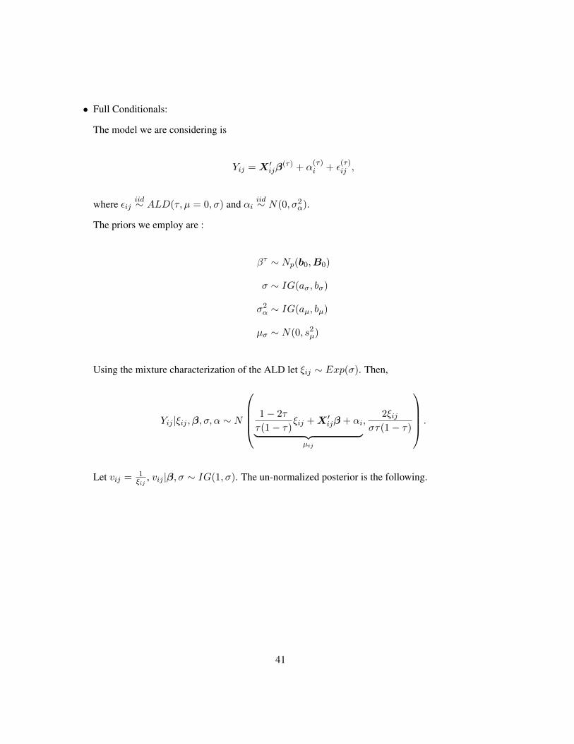
• Full Conditionals:
The model we are considering is
Yij = X ′ijβ(τ) + α
(τ)i + ε
(τ)ij ,
where εijiid∼ ALD(τ, µ = 0, σ) and αi
iid∼ N(0, σ2α).
The priors we employ are :
βτ ∼ Np(b0,B0)
σ ∼ IG(aσ, bσ)
σ2α ∼ IG(aµ, bµ)
µσ ∼ N(0, s2µ)
Using the mixture characterization of the ALD let ξij ∼ Exp(σ). Then,
Yij |ξij ,β, σ, α ∼ N
1− 2τ
τ(1− τ)ξij +X ′ijβ + αi︸ ︷︷ ︸µij
,2ξij
στ(1− τ)
.
Let vij = 1ξij
, vij |β, σ ∼ IG(1, σ). The un-normalized posterior is the following.
41

π(β, σ, σ2α, µα,α|y,X) ∝ `(β, σ, v, α; y,X)π(β, σ, v, α, σ2α)
∝m∏i=1
ni∏j=1
(σvijτ(1− τ))1/2 exp
{−1
2
σvijτ(1− τ)
2(yij − µij)
}
× exp
{1
2(β − b0)′B−10 (β − b0)
}× IG(vij , 1, σ)×G(σ, aσ, bσ)× IG(σ2α, aµ, bµ)×
{m∏i=1
exp
{− 1
2σ2αα2i
}}
Letting V = 2στ(1−τ)diag(v11, . . . , vm,nm),U = (Y11− 1−2τ
τ(1−τ)v11 , . . . , Ymnm −1−2τ
τ(1−τ)vmnm), and
α = (α1, . . . , αm), the full conditionals are
[β|−] ∼ N[(X ′V −1X +B−10 )(U ′V −1X −α′V −1X + b′0B
′0), (X
′V −1X +B−10 )−1]
[σ|−] ∼ IG
3N/2 + aσ + 1,1
2
τ(1− τ)
2
∑ij
vij(yij − µij)2 +∑ij
vij + 1/bσ
[αi|−] ∼ N
(12σ τ(1− τ)[
∑j vij(Yij −X ′β)− ni(1− 2τ)] + 1
σ2αµα
12σ τ(1− τ)
∑j vij + 1
σ2α
,1
12σ τ(1− τ)
∑j vij + 1
σ2α
)
[σ2α|−] ∼ IG
(0.5m+ aα,
1
2
∑i
(αi − µα)2 + 1/bα
)
[µα|−] ∼ N
(1σ2α
∑i αi
mσ2α
+ 1s2µ
,1
mσ2α
+ 1s2µ
)
[vij |−] ∼ InvGauss
(1
τ(1− τ)|Yij −X ′ijβ − αi|,
1
2στ(1− τ)
)
42