1

Exploring a new technique to determine the optimal

real estate portfolio allocation

by

Tingting Fu

B.S., Economics, 2004

Xi’an Jiaotong University

Submitted to the Program in Real Estate Development in Conjunction with

the Center for Real Estate on January 17, 2014 in Partial Fulfillment of the

Requirements for the Degree of Master of Science in Real Estate

Development

at the

Massachusetts Institute of Technology

February, 2014

©2014 Tingting Fu

All rights reserved

The author hereby grants to MIT permission to reproduce and to distribute publicly

paper and electronic copies of this Thesis document in whole or in part in any medium

now known or hereafter created.

Signature of Author____________________________________________________________

Program in Real Estate Development

January 17, 2013

Certified by___________________________________________________________________

Walter N. Torous

Senior Lecturer of Center for Real Estate and Sloan School of Management

Thesis Supervisor

Accepted by___________________________________________________________________

David Geltner

Chairman, Interdepartmental Degree Program in Real Estate Development

2

(Page left blank intentionally)

3

Exploring a new technique to determine the optimal real estate portfolio

allocation

by

Tingting Fu

Submitted to the Program in Real Estate Development in Conjunction with

the Center for Real Estate on January 17, 2014 in Partial Fulfillment of the

Requirements for the Degree of Master of Science in Real Estate

Development

Abstract

Modern Portfolio Theory has been developed over the last fifty years, and there

are several studies linking Modern Portfolio Theory with the allocation of real

estate property in multi-asset portfolios. However, in reality, most real estate

fund managers don’t use MPT as a guideline when they are structuring a

portfolio and deploying allocation strategy for a real estate fund. The main

reason for this gap between theory and reality is that the traditional mean-

variance approach of MPT requires accurate data of variances, covariance and

expected return over the long term; and those data are quite difficult to collect

on an ad hoc base.

This Thesis applies a new technique to examine property asset allocation

strategies and improve the performance of a real estate investment sample

portfolio in the US. We straight-model the portfolio weight in each property type

of asset as a function of the asset’s characteristics: either physical attributes such

as property size, vacancy rate, property type, location etc.; or financial attributes

such as Cap Rate. The coefficients of this function are found by optimizing the

investor’s average utility of the portfolio’s return over a certain period of years.

The aim of this approach is to find a simple and easily modified methodology for

real estate portfolio managers when they are deciding on acquisitions and

making portfolio policies.

In general, this Thesis aims to apply the new technique to help practitioners and

other researchers improve the practical implementation of optimal portfolio

policies.

Thesis Supervisor: Walter N. Torous

Title: Senior Lecturer of Center for Real Estate and Sloan School of

Management

4

Table of Contents

ABSTRACT ................................................................................................................................................................................ 3

ACKNOWLEDGEMENTS ..................................................................................................................................................... 7

CHAPTER 1: INTRODUCTION .......................................................................................................................................... 8

1.1 THEORY REVIEW ............................................................................................................................................................ 8

1.2 STATUS QUO .................................................................................................................................................................... 8

CHAPTER 2: METHODOLOGY ........................................................................................................................................ 12

2.1 BASIC IDEA .................................................................................................................................................................... 12

2.2 DATA .............................................................................................................................................................................. 13

2.2.1 Data Sources and Portfolio Creation ..................................................................................................... 13

2.2.2 Variables Selections ...................................................................................................................................... 14

2.3 Objective function ............................................................................................................................................. 17

2.4 Portfolio Weight Constraints ........................................................................................................................ 20

2.5 Other time varying coefficients ................................................................................................................... 21

CHAPTER 3: EMPIRICAL APPLICATION AND RESULTS .................................................................................... 23

3.1 DATA DESCRIPTION ...................................................................................................................................................... 23

3.1.1 Market Value: ................................................................................................................................................... 24

3.1.2 Size: ...................................................................................................................................................................... 25

3.1.3 Cross Sectional Average Price .................................................................................................................. 26

3.1.4 Time-series total return (Quarterly) ..................................................................................................... 28

3.1.5 Property type ................................................................................................................................................... 29

3.1.6 Geographic location ...................................................................................................................................... 29

3.2 STATISTICS SUMMARY ................................................................................................................................................. 32

3.3 RESULTS ......................................................................................................................................................................... 34

3.3.1 Four variables .................................................................................................................................................. 34

3.3.2 Consideration of locations ......................................................................................................................... 36

3.3.3 More variables .......................................................................................................................................... 38

3.3.4 Snapshot for each quarter ................................................................................................................... 40

3.4 Extension ....................................................................................................................................................... 43

5

CHAPTER 4 CONCLUSION ............................................................................................................................................... 44

APPENDIX 1 ........................................................................................................................................................................... 45

APPENDIX 2 ........................................................................................................................................................................... 49

REFERENCES ......................................................................................................................................................................... 52

6

7

Acknowledgements

I would like to take this opportunity to thank those people who have been

generously providing help to me since I moved to the United States.

This Thesis could not have been completed without the advice and support of

many people and organizations. Before I extend my appreciation, I would like to

sincerely thank my Thesis advisor Professor Walter Torous for his guidance and

support throughout the entire process. The entire concept of this Thesis is

inspired by Professor Torous and his fellow Professors Alberto Plazzi and

RossenValkanov. Also, I would like to thank Professor David Geltner for

generously sharing with me his comments, opinions and resources to help me

overcome barriers on the way. Last but not least, I would like to thank my

academic advisor Professor William Wheaton for sharing with me his

connections and for pushing me to become a stronger person by his wisdom,

knowledge and experience.

I also would like to thank the various real estate investment firms for sharing

with me their data necessary to complete this Thesis and portfolio managers

who accepted my interviews and shared with me their experiences and thoughts

of the industry. The names of the firms and individuals who have assisted will

not be specified so as to maintain confidentiality, however, I would like to thank

them for their generosity and willingness to provide data to me. This Thesis

definitely would not have been able to be completed without their support.

I would especially like to express my appreciation to my fellow classmates, and

the faculty and staff of MIT Center for Real Estate. Because of them, the past one

and a half years have been such a memorable and enriching experience in my

life. Many alumni of CRE helped me to explore the ideas of this Thesis and

provided valuable input, with special thanks to Pulkit Sharma, Arvind Pai,

Jonathan Richter and Peter McNally. Additional thanks to Beipeng Mu and Ermin

Wei for teaching me how to use Matlab, a new mathematics tool to me, and for

encouraging me to keep exceeding my limits.

Finally, I would like to thank my parents for their unconditional support,

encouragement and love along the way. They are my role models, and they are

the persons who teach me independence, perseverance, bravery, giving and love.

8

Chapter 1: Introduction

1.1 Theory Review

Based on traditional investment theory, we learn that investors should diversify

their investment portfolio in order to reduce total risk at a given level of return

and risk. Classic Modern Portfolio Theory (MPT) provides a perfect theoretical

framework for this process. The basic concept of MPT is that diversification is

achieved not only by investing in an increased number of investments, but also

by investing in a number of assets whose pattern of returns are distinct and

different enough from each other to partially or wholly offset each other’s

returns and therefore reduce overall portfolio volatility.

The most widely used approach generated from MPT is the “mean- variance

approach” developed by Markowitz (1952). This approach has been used to

determine an optimal portfolio allocation. An optimal portfolio of assets is

selected by combining an efficient frontier with a specification of the investor’s

preferences for risk and return. According to Getlner, Miller, Clayton and

Eichholtz’s book Commercial Real Estate Analysis and Investment, MPT makes

three major contributions: (1) it treats risk and return together in a

comprehensive and integrated manner; (2) it quantifies the investment-decision-

relevant implications of risk and return; and (3) it makes both of these

contributions at the portfolio level, the level of the investor’s overall wealth.

Experimental results of portfolio management also testify that certain

combinations of assets are more valuable than others due to their higher returns

with lower risk levels than others as far as their diversification effect is

concerned.

1.2 Status Quo

Despite the benefits of a formal portfolio optimization approach such as MPT, in

reality, such an approach is seldom implemented by fund managers regardless of

whether they are investing in traditional stocks and bonds or other alternative

investments, like real estate. The main reason of this gap between theory and

reality is that the traditional mean-variance approach requires accurate data of

9

variances, covariance and expected return over the long term, and those data are

quite difficult to collect on an ad hoc base.

In practice, most asset allocation decisions must be made in the context of

incomplete information, changing estimates of return, and shifting definitions of

the acceptable investment risk. Significant amount of uncertainty about the true

underlying assets in return-generated processes makes it difficult for investors

and fund managers to execute the traditional mean-variance method. On the

other hand, even when fund managers and researchers are able to make

reasonable assumptions and collect reliable data of variances, covariance and

expected return, when the traditional mean-variance method has been

implemented to optimize portfolio weights in a large number of assets it tends to

create notoriously noisy and unstable results.

If that is the case, then, how do real estate fund managers construct their

portfolios in their daily practices? Is there an easier method existing which they

are able to apply? To answer this question, in the past five months, I interviewed

seven real estate portfolio managers who work in the real estate open-ended

fund business in the US. In terms of the interviewees’ background, four of them

work for real estate investment firms and three of them work for the real estate

management teams of investment banks. After studying and compiling the

records of the interviews, a few common results about the decision-making

processes of acquisitions and asset selection were identified, and have been

described in this Thesis.

Six of seven portfolio managers mentioned that their allocation process was

influenced by certain non-financial considerations, such as behavioral issues.

They use their own judgment, experiences and creativity to make a property

allocation investment decision. Most of the portfolio managers I interviewed

have been working in the industry for a long time, generally over 20 years. And

for them, the most common investment technique they used in their daily

practice for real estate allocation was just general experience and intuition.

Other behavioral issues involve the level of aggressiveness of investment

brokers. Two interviewees mentioned that the decisions of portfolio managers

and acquisitions managers could be heavily influenced by investment brokers’

strong intention to sell one specific property instead of another. The marketing

10

materials investment brokers provided to institutional buyers also tend to favor

a brokers’ particular preference.

Some portfolio managers determine future property allocation by benchmarking

from their current allocation. The primary reason of doing this is because of the

fact that they see their current allocation as conceptually a safe base, and it thus

becomes a benchmark from which the institution deviates as new information

becomes available.

The conclusion generated from interviews is that although there is extensive use

of hard information from the market, the use of personal “gut-feeling” as to the

state of the market and information based on the views of others is commonly

adopted in a decision-making process. Besides gut-feeling, a recent research

report in Institutional Real Estate, Inc (2013) December 1, 2013: Vol. 25, Number

11 also found that the use of asset consultants in the real estate investment

strategies for US pension funds and insurance firms is commonplace as well.

Asset consultants advise US pension funds and other institution investors on

portfolio strategy, performance monitoring and property selection. They tended

to contribute more evidently at the strategic level as well as in the allocation of

direct property investment versus listed property and listed vehicle selections

on the public market.

Meanwhile, unlike other asset types in the traditional finance market, for

example stocks or bonds, the real estate acquisition decisions tend to heavily rely

on the availability of potential opportunities in the market. Even given portfolio

policy, allocation decisions could be strictly constrained by the available

alternatives on the market. As we can imagine, all of those factors we mentioned

in last few paragraph could be barriers to keep a real estate portfolio from

achieving the optimized solution. And importantly, even in a perfect theoretical

world, the optimized solution for real estate portfolio is very difficult to measure

as well.

We learned from interviews and research that portfolio managers like to use

qualitative methodology to construct their funds, but how about quantitative

techniques of portfolio management? If MPT theory existed only in the academic

world, are there other quantitative techniques or methods that have been and

are used?

11

We received positive feedback from interviews on this question as well. A few

numerical indicators have been widely used to measure ad hoc performance of

real estate funds, and most fund managers make reference to a series of risk and

return evaluation measures when evaluating their property asset allocation

decision. Certain quantitative techniques, for example Internal Rate of Return

(IRR), are one of the most important and popular return evaluation measures.

Initial yield also has been identified as a frequently used measure of property

return. Some institutional investors also calculate cash-on-cash return.

Sensitivity analysis, debt coverage ratio and scenario analysis are also popular

quantitative risk assessment techniques.

In general, the most popular quantitative measurements for property return that

real estate portfolio managers applying practice are IRR and initial yield.

Sensitivity analysis is often used as the risk analysis tool. However, from the

interviews I conducted, I did not learn of any quantitative techniques regarding

portfolio diversification, which indicates that there might be space for applying

and developing this technique in the diversification methodology of real estate

practices.

12

Chapter 2: Methodology

2.1 Basic Idea

The quantitative technique originally comes from the traditional finance market.

To avoid exploiting facts about stocks’ characteristics, such as a firm’s book to

market ratio or its stock’s lagged return, variance and covariance as compared

with other stocks, Brandt, Santa-Clara and Valkanov developed a novel approach

in 2009 to optimizing portfolios with large numbers of assets in the stock

market.

They applied this new methodology to equity portfolio optimization based on a

firm’s characteristics. They parameterize the portfolio weight of each stock as a

function of the firm’s characteristics, and estimate the coefficients of the

portfolio policy by maximizing the average utility the investor would have

obtained by implementing the policy over the historical sample period.

(“Parametric Portfolio Policies: Exploiting Characteristics in the Cross-Section of

Equity Returns 10996”)

Commercial Real Estate as a critical asset type oftentimes triggers people to

think about whether it is possible to develop techniques similar to those used in

the financial market to quantify the effect of property characteristics on a real

estate portfolio? Instead of relying heavily on their experience and judgment

(“gut–feeling”), whether there exists an applicable methodology which fund

managers could simple and easily use in their daily work when they select a real

estate portfolio?

In past two or three years, a few pioneering researchers have explored the

possibilities for the optimization of a real estate portfolio from a mathematically-

based methodology. The major purpose of doing this type of exploration is to

simplify the portfolio allocation processes and to answer a number of unsettled

questions in the management of commercial real estate portfolios; for example,

how should investors allocate their capital across different commercial

properties based on a mathematic, scientific calculation? How does the risk-

13

return profiles of offices, hotels, residential and retail properties differ from one

another? How should investors alter the composition of their commercial real

estate portfolios to take advantage of movements in expected returns arising

from changing underlying macroeconomic conditions?

Plazzi, Torous, and Valkanov started exploring a new methodology to apply this

quantitative technique to the real estate market since 2010. Based on this

previous work, this Thesis aims to further apply and extend this new

methodology with the objective of optimizing real estate fund managers’

decision processes and of improving fund’s performance.

2.2 Data

2.2.1 Data Sources and Portfolio Creation

To make this quantitative technique approach more similar to investment

practices in the real world, instead of using open sources data like NCREIF NPI

index, we used the data gathered from several managed real estate funds in the

institutional investment industry to discuss and examine the proposed

techniques. The various funds that provided data to further this research came

together cooperatively and anonymously to explore the use of this new

technique, taking on the role collectively as the “client” of the Thesis, based on

their belief that they all shared common strengths, weaknesses and constraints,

as well as a similar organizational context.

Considering the similarities in the various own-account funds in terms of risk

and return requirements, in this Thesis, we are treating all of the property

investment cases as if they came from a single investment management firm for

purposes of analyzing and interpreting this property characteristics technique.

We would like to call this technique the Property Characteristics Technique

(PCT). For the sake of convenience, the source of the data pool analyzed in this

Thesis will be referred to going forward as the “Investment Portfolio”.

14

The Investment Portfolio data began in 1978 Q4 and ends at 2013 Q2. The

disaggregated information includes property’s location and asset type, property

market value, net operation income and total return. In terms of market value,

if a property is sold during a certain period, we use the actual selling price as

market value. If it is still in the portfolio, we use an appraisal value calculated by

a third party appraiser firm as the market value of the property. The total return

is calculated by investment firm’s in-house appraiser teams applying the same

methodology.

2.2.2 Variables Selections

To simplify the process of asset allocation and acquisitions decisions and to

make it easier for portfolio managers to apply in their daily practices, we have to

select intuitive parameters as variables for the PCT model. Meanwhile, in order

to be relevant, these variables have to be varied in the investment portfolio

either cross-sectionally or by time series.

As the key purpose of this technique is to maximum portfolio returns, the PCT

model investigates whether a portfolio allocation policy across different types of

assets can be improved by adjusting conditional variables. Therefore, one of the

essential principles of selecting variables is its relevance to the total estimated

return of a particular real estate portfolio. Based on economic theory, the study

of previous researchers’ research papers and data availability, we use the

conditional variables below to construct our model.

CAP RATE: Cap Rate is the ratio between the net operating income produced by

a property and its current market value. There are a number of researchers that

have proved the correlation between Cap Rate and return. The Cap Rate, that is,

the rent-price ratio in commercial real estate, captures fluctuations in expected

returns for apartments, retail, as well as industrial properties. For offices, by

contrast, Cap Rate does not forecast returns even though expected returns on

offices are also time-varying. (Plazzi, Torous, & Valkanov, 2010)

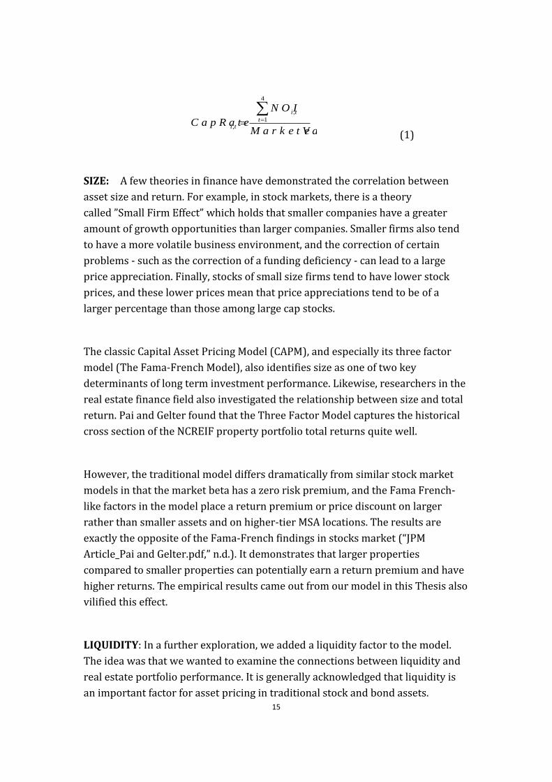
We use tiNOI , to represent building i’s NOI in time t. Given that the available

data in our investment portfolio is on a quarterly basis, we calculate the

property’s Cap Rate according to the below formula:

15

eM a r k e t V a l u

N O I

C a p R a t e t

ti

ti

4

1

,

,

(1)

SIZE: A few theories in finance have demonstrated the correlation between

asset size and return. For example, in stock markets, there is a theory

called ”Small Firm Effect” which holds that smaller companies have a greater

amount of growth opportunities than larger companies. Smaller firms also tend

to have a more volatile business environment, and the correction of certain

problems - such as the correction of a funding deficiency - can lead to a large

price appreciation. Finally, stocks of small size firms tend to have lower stock

prices, and these lower prices mean that price appreciations tend to be of a

larger percentage than those among large cap stocks.

The classic Capital Asset Pricing Model (CAPM), and especially its three factor

model (The Fama-French Model), also identifies size as one of two key

determinants of long term investment performance. Likewise, researchers in the

real estate finance field also investigated the relationship between size and total

return. Pai and Gelter found that the Three Factor Model captures the historical

cross section of the NCREIF property portfolio total returns quite well.

However, the traditional model differs dramatically from similar stock market

models in that the market beta has a zero risk premium, and the Fama French-

like factors in the model place a return premium or price discount on larger

rather than smaller assets and on higher-tier MSA locations. The results are

exactly the opposite of the Fama-French findings in stocks market (“JPM

Article_Pai and Gelter.pdf,” n.d.). It demonstrates that larger properties

compared to smaller properties can potentially earn a return premium and have

higher returns. The empirical results came out from our model in this Thesis also

vilified this effect.

LIQUIDITY: In a further exploration, we added a liquidity factor to the model.

The idea was that we wanted to examine the connections between liquidity and

real estate portfolio performance. It is generally acknowledged that liquidity is

an important factor for asset pricing in traditional stock and bond assets.

16

Kawaguchi, Sa-Aadu, Shilling used time series data from 1982 to 1998 to show

that there is indeed an apparently substantial illiquidity effect in commercial

property returns – less liquidity implies a higher expected return for

institutional investors.

The consequence pattern that comes from their model appears just as strong as

the pattern in stock returns. This is an interesting result, given that the holding

period for commercial real estate is generally far longer than the holding period

for stocks (“Do Changes in Illiquidity Affect Investors’ Expectations”). For this

liquidity analysis, we divided properties into two groups according to their

geographic locations: Top- 6 cities and non-Top- 6 cities. Top- 6 cities include

New York, Boston, Washington DC, LA, San Francisco and Chicago.

PROPRERTY TYPE. Traditional theory on diversification strategies advocated

that property type is an important diversification criteria for institutional

investors. Historically, scholars have been exploring the optimization of property

type allocation in portfolio performance. Firstenberg, Ross and Zisler in their

paper “Real Estate: The Whole Story” (1988), use Frank Russell (FRC) AND

Evaluation Associates (EAFPI) return index series to examine how diversification

within property types and geographic locations effects estimated return. They

concluded that diversifying the composition of a portfolio among geographic

locations and property types can increase the investor’s return for a given level

of risk.

Pai and Getlner also find that property type (Office, Hotel, Apartment, Industrial,

etc.) is a very powerful predictor of long-term average investment performance

even controlling for the risk factors is considered. (“JPM Article_Pai and Gelter”)

This finding is in favor of us using property type as another variable to measure

total return.

Risk: There is a negative correlation between the risk of a real estate portfolio

and total expected return. Risk is usually measured as volatility and standard

deviation. Undoubtedly, the degree of risks that investors are willing to take

represents one of the most important factors in determining expected return.

Different investors have various risk appetites. In our Property Characteristics

Technique model, we use three numbers to represent different kinds of

investors.

17

The optimal portfolio heavily depends on the investor’s preferences. Therefore,

we assume CRRA utility function with risk aversion equal to 5 as normal risk

aversion level. Besides equals 5, we also report the result when equals 9

which represent the investors who are extremely sensitive to losses, like pension

fund and other conservative investors. In additional, we also calculate the

scenario that when equals 2, which represents the investors who have high

risk appetite like hedge funds.

The PCT model we created in this Thesis can be applied to examine the

importance of other property characteristics in commercial real estate portfolio

allocation as well. For example, the conditional variables could be extended to

transaction cost, vacancy rate, and capital expenditure etc. For most portfolio

managers, they might also like to know the importance of each market friction

that might occur. Depending on the requirements of the individual portfolio

manager, the model could be tailor-made to a more practical format.

2.3 Objective function

The basic approach of PCT is to set up a utility function in associated return with

a vector of buildings characteristics. For example, we suppose that at any

particular time (t), there is a large number (Nt ) of buildings in the portfolio. Each

building (i) has a return of tir , from time (t) and is associated with a vector of

the building’s characteristics ( tix , ) observed at time (t). The property

characteristics could be physical attributes of the buildings or financial attributes

of the assets. In this Thesis, we select Cap Rate, Size, Liquidity and Property Type

as our characteristics. The key task for a portfolio manager is to choose the

weights ti ,to maximize the conditional expected utility of portfolio return tPr ,

To differentiate the return of an individual property from the return of the

overall portfolio, we use tPr , to represent the return of the portfolio and tpr , to

represent the return of the individual property.

18

)]([)]([max ,

1

,,}{ 1,

ti

N

t

tittptw

ruEruEt

tNiti

(2)

The optimal portfolio weights can be parameterized as a linear function of

buildings characteristics.

);( ,, titi

xf

ti

t

ti xN

,

'

,

1

(3)

ti , is the weight of building i at time t in a benchmark portfolio. In this Thesis, I

use a market value weighted portfolio as a benchmark, which means using the

market value to calculate the weight of each individual property in the portfolio.

is a vector of coefficients to be estimated and tix , are the characteristics of

buildings. The vector of coefficients reflects deviations between current

portfolio allocations with optimal portfolio allocation (QUESTION: Is this

between two different allocations?), and therefore, indicates the importance of

property selections. The intercept ti , is the weight of the building in a

benchmark portfolio while the tix ,

'represents the deviations of the optimal

portfolio weight from this benchmark. tN

1

is a normalization that enables the

portfolio weights function to be applied to any arbitrary and time-varying

number of buildings.

Constant coefficient' is undoubtedly the most critical aspect in the

parameterization. It implies that the portfolio weight in each building depends

only on the building’s characteristics and not on the property’s historic return.

Constant coefficients through time mean that the coefficients that maximize the

investor’s conditional expected utility at a given date are the same for all dates

and therefore also maximize the investor’s expected utility.

If we put back all the variables we selected in 2.2.2, the linear function would be

written as:

19

);( ,, titi

xf

ti

t

ti xN

,

'

,

1

(3)

= )6[(1

6,,, industrialtopsizecapN

industrialtoptisizeticap

t

ti

The key part of the modeling optimization process is to select the investors’

objective function. Unlike traditional mean variance methods, the specification of

the portfolio selection can adopt any choice of objective function as long as the

function can be specified with a unique solution. For example, (“Parametric

Portfolio Policies: Exploiting Characteristics in the Cross-Section of Equity

Returns 10996”) Brandt, Santa-Clara and Valkanov, in their paper, mentioned

that this method could be applied to behaviorally motivated utility functions

such as loss aversion, ambiguity aversion, or disappointment aversion, as well as

practitioner-oriented objective functions, including maximizing the Sharpe or

information ratios, beating or tracking a benchmark, controlling drawdowns, or

maintaining a certain value at risk.

From a practical perspective, we use the standard Constant Relative Risk-

Aversion (CRRA) utility function in this thesis.

1

)1()(

1

,

,

tp

tp

rru

(4)

If we incorporate the expected return algorithms for this specified utility

function, the optimization problem could be revised to:

T

t

tpT

t

tp

r

Tru

T 1

1

,

1

,1

)1(1max)(

1max

tatb

Nt

i

titti

T

titP

rr

rNxr

,,

1

,,,, )/(

(5)

20

tbr , represents the return of each property in the benchmark portfolio and tar ,

represents the deviation of return in the benchmark portfolio and the optimal

portfolio. The CRRA utility function as compared with other functions could

bring preferences towards higher order moments in a more discreet manner.

2.4 Portfolio Weight Constraints

To avoid using strictness constraints so as to generate an optimal solution, the

easiest constraint we could use in this optimization is non-negative weights.

There are a few alternative ways of expressing non-negative constraints in

portfolio weight. In order to be applicable to the real estate market, where

shorting is not very common, we use the below constraint:

Nt

i

ti

ti

ti

1

,

,

,

],0max[

],0max[

(6)

Additionally, if we look back at function (2), we have to keep both the sum of

weights in the benchmark portfolio and the weight of the optimization portfolio

equal to one.

);( ,, titi

xf

ti

t

ti xN

,

'

,

1 (3)

To meet the condition that 1, ti and 1, ti

, the sum of ti

t

xN

,

'1

has to

equal to zero. Therefore, it generated our second constraint that:

21

01

0

,

'

n

t

ti

t

xN

(7)

2.5 Other time varying coefficients

Some of you might be wondering whether the constant coefficients of portfolio

through time is reasonable? From an academic perspective, it is a very

convenient assumption because it avoids some difficult statistics techniques.

However, there is substantial evidence showing that macroeconomic variables as

related to business cycles are highly related to forecasts of the aggregate

properties returns.

To accommodate possible time varying macroeconomic factors, we can simply

add those factors as one of the variables to the function. With it in mind, we need

to consider that macroeconomic factors have a complicated influence on each

variable in the function. To achieve this goal, we can use Kronecker Product to

reflect that the impact of the properties’ characteristics on the portfolio weight

varies with the influence of macroeconomic and business cycle variables. We can

choose the US National Statistics Bureau’s annual GDP index and other relevant

indexes as these variables.

To match our quarterly basis data and for the sake of preciseness, we choose

CFNAI as one of the macroeconomic indicators. CFNAI is the Chicago Fed

National Activity Index, which is a monthly index designed to gauge overall

economic activity and related inflationary pressure. The CFNAI is a weighted

average of 85 existing monthly indicators of national economic activity. It is

constructed to have an average value of zero and a standard deviation of one.

Since economic activity tends toward trend growth rate over time, a positive

index reading corresponds to growth above trend and a negative index reading

corresponds to growth below trend.

The 85 economic indicators that are included in the CFNAI are drawn from four

broad categories of data: production and income; employment, unemployment,

22

and hours; personal consumption and housing; and sales, orders, and

inventories. Each of these data series measures some aspect of overall

macroeconomic activity. (According to CFNAI’s official website:

http://www.chicagofed.org/webpages/publications/cfnai/)

Therefore, the linear function of weight can be revised to:

])6[(1

)(1

);(

6,,,

,

'

,

,,

tindustrialtoptisizeticap

t

ti

tti

t

ti

titi

zindustrialtopsizecapN

zxN

xf

(8)

Where we use Z to represent economics factor and ⊗ for the Kronecker Product,

which is an operation on two matrices of arbitrary size resulting in a block

matrix. It is a generalization of the outer product from vectors to matrices, and

gives the matrix of the tensor product with respect to a standard choice of basis.

(Cited from Wikipedia: http://en.wikipedia.org/wiki/Kronecker_product)

23

Chapter 3: Empirical Application and Results

3.1 Data description

To implement the theoretical idea that we illustrated in the first two chapters,

we use investment portfolio data to present an empirical application of this

technique. We use quarterly property level returns in the investment portfolio as

well as property level characteristics including market value, Cap Rate, location

information, size, NOI etc. The data set begins at 1978 Q4 and ends at 2013 Q2.

We are going to describe the data first and then release the results after running

optimization through Matlab, a numerical computing environment and

programming language that has been widely used as quantitative analysis tool

and optimization software. We are going to report the data under three different

levels of risk aversion. In this Thesis, we assume that all the properties in the

portfolio involve different level of risks and risk-free assets are not included in

this portfolio.

We construct the data set at the end of each year, which consists of four (4)

quarters of data. The number of building in the investment portfolio is

continuously increasing, although a few buildings have been sold out after

property holding period. The average annual rate of increase in the number of

buildings is 2.05% from 1978 Q4 to 2013 Q2. The average number of buildings

throughout the duration of the investment portfolio is ninety-four (94)

properties, with the fewest number twenty-one (21) in 1978 Q4, and the greatest

number two hundred forty-five (245) in 2013 Q2.

Below are a number of graphs to describe the cross sectional average and

standard deviation of Cap Rate, size and market value of the properties.

Additionally, we use graphs to illustrate the cross sectional price per square foot

of the properties. Appendix 1 provides further details about the property-level

data, including the exact definitions of the components of each variable. We use

size, Cap Rate, industrial and Top- 6 city as conditioning characteristics in the

portfolio optimization according to their relevance and data availability.

24

3.1.1 Market Value:

Figure 1 describes Total Market Value,

Average Market Value, and Market

Value by each property type and

Market Value Comparison across all

types of property.

To help us understand how large this portfolio is from 1978 to 2013, Figure 1

describes the total market value, average market value and market value for each

type of property in the portfolio. Looking at the general trend of the portfolio, the

market value is increasing throughout its duration, with a significant increase

25

since 2000. It has a downturn in 2009 and rises again ever since. The last graphs

in Figure 1 also show the proportion of market value for each type of property.

Office buildings weight the most value in the whole portfolio and hotels are the

smallest portion of the assets from a market value perspective.

3.1.2 Size:

Figure 2 describes the aggregate size

trend in each quarter from 1978 to

2013.

26

3.1.3 Cross Sectional Average Price

According to the average price analysis of five types of properties, only industrial

properties have obvious patterns that correspond with macroeconomic cycles.

Whereas with the other four types of properties, (office, retail, apartment and

hotel), in general, the average prices are increasing and could generate both

linear and exponential forecasts.

Figure 3 describes the average price by

each property type.

Let us have a close look at the average price for each single property type. The

average price of industrial property shows a significant cyclical pattern, whereas

with the other four types of properties, the earnings trend upwards generally.

Those four types of properties have significant, above-average increases from

27

2004 to 2008, and under-average price increases from 1999 to 2002 and 2009 to

2012.

28

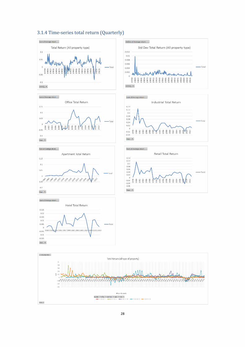
3.1.4 Time-series total return (Quarterly)

29

Figure 4 describes quarterly total return on each type of asset and comparison

among different asset types.

Since we already know the quarterly return of individual properties from the

original data, we could use the aggregate return to calculate overall return as

well as return for each property type on a value weight basis, where the

individual property’s weight is proportional to its market value. ir represents

the return for each individual building and Pr represented the return of the

portfolio. The returns of particular property types have been donated by officer

hotelr industrialr retailr apartmentr . By comparing these returns with certain

macroeconomic return charts, we note that it roughly matches with

macroeconomic cycles.

3.1.5 Property type

There are five property types included in the investment portfolio we are

analyzing in this Thesis: Industrial, Office, Apartment, Retail and Hotel. The

predominant type of property in the portfolio is Industrial. Therefore we choose

Industrial versus non-Industrial property as one of the standardized variables in

the portfolio function to examine how the variation of property type may cause

changes in the return of the portfolio.

3.1.6 Geographic location

To better illustrate the geographic location distributions of this portfolio and

examine the impact of these distributions on the performance of the portfolio,

we only select properties which are located in the US. We use Excel to make a 3-

D data visualization model of these properties and mark out all the location

distributions of each asset by size and filtered with property type. According to

the regional divisions used by the US Census Bureau, we divided all the states into

four areas: Northeast, Midwest, South and West.

Northeast includes: Maine, New Hampshire, Vermont, Massachusetts, Rhode

Island, Connecticut, New York, Pennsylvania, and New Jersey

30

Midwest includes: Wisconsin, Michigan, Illinois, Indiana, Ohio, Missouri, North

Dakota, South Dakota, Nebraska, Kansas, Minnesota, and Iowa

South includes: Delaware, Maryland, District of Columbia, Virginia, West Virginia,

North Carolina, South Carolina, Georgia, Florida, Kentucky, Tennessee,

Mississippi, Alabama, Oklahoma, Texas, Arkansas, and Louisiana

West include: Idaho, Montana, Wyoming, Nevada, Utah, Colorado, Arizona, New

Mexico, Alaska, Washington, Oregon, California, and Hawaii

31

32

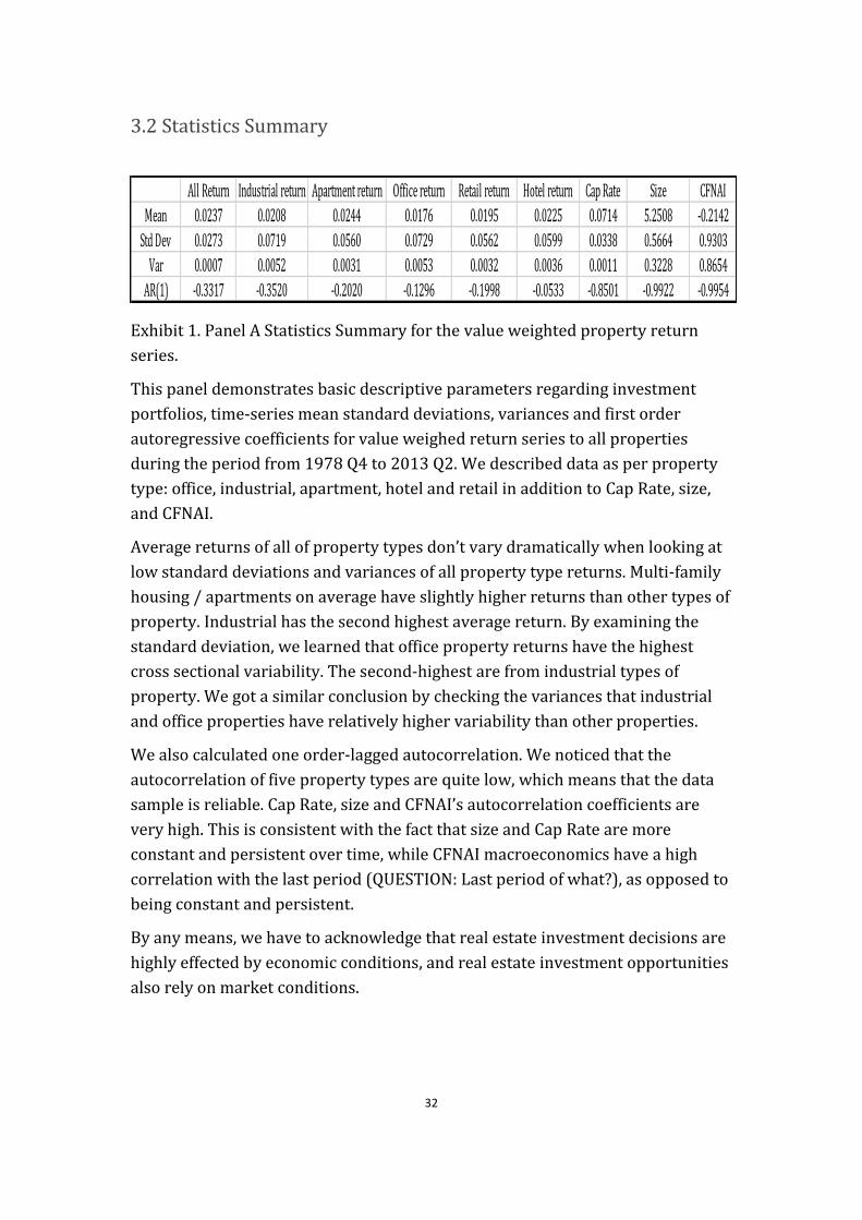
3.2 Statistics Summary

Exhibit 1. Panel A Statistics Summary for the value weighted property return

series.

This panel demonstrates basic descriptive parameters regarding investment

portfolios, time-series mean standard deviations, variances and first order

autoregressive coefficients for value weighed return series to all properties

during the period from 1978 Q4 to 2013 Q2. We described data as per property

type: office, industrial, apartment, hotel and retail in addition to Cap Rate, size,

and CFNAI.

Average returns of all of property types don’t vary dramatically when looking at

low standard deviations and variances of all property type returns. Multi-family

housing / apartments on average have slightly higher returns than other types of

property. Industrial has the second highest average return. By examining the

standard deviation, we learned that office property returns have the highest

cross sectional variability. The second-highest are from industrial types of

property. We got a similar conclusion by checking the variances that industrial

and office properties have relatively higher variability than other properties.

We also calculated one order-lagged autocorrelation. We noticed that the

autocorrelation of five property types are quite low, which means that the data

sample is reliable. Cap Rate, size and CFNAI’s autocorrelation coefficients are

very high. This is consistent with the fact that size and Cap Rate are more

constant and persistent over time, while CFNAI macroeconomics have a high

correlation with the last period (QUESTION: Last period of what?), as opposed to

being constant and persistent.

By any means, we have to acknowledge that real estate investment decisions are

highly effected by economic conditions, and real estate investment opportunities

also rely on market conditions.

All Return Industrial return Apartment return Office return Retail return Hotel return Cap Rate Size CFNAI

Mean 0.0237 0.0208 0.0244 0.0176 0.0195 0.0225 0.0714 5.2508 -0.2142

Std Dev 0.0273 0.0719 0.0560 0.0729 0.0562 0.0599 0.0338 0.5664 0.9303

Var 0.0007 0.0052 0.0031 0.0053 0.0032 0.0036 0.0011 0.3228 0.8654

AR(1) -0.3317 -0.3520 -0.2020 -0.1296 -0.1998 -0.0533 -0.8501 -0.9922 -0.9954

33

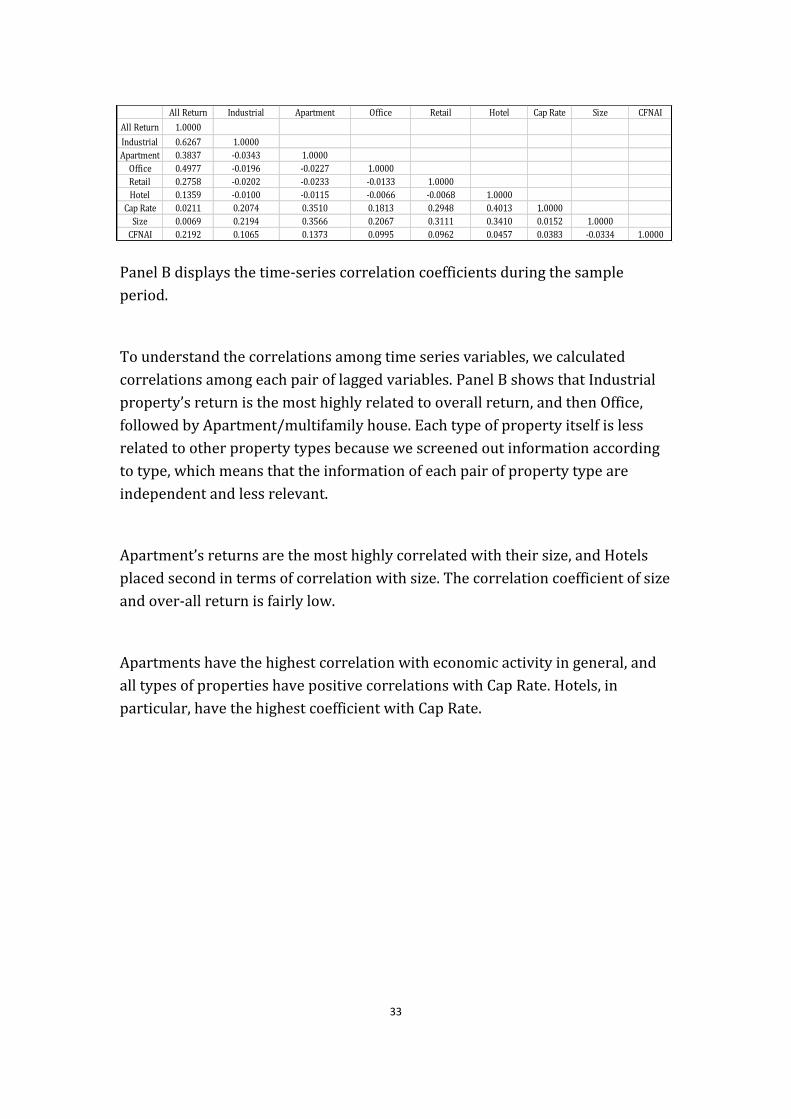
Panel B displays the time-series correlation coefficients during the sample

period.

To understand the correlations among time series variables, we calculated

correlations among each pair of lagged variables. Panel B shows that Industrial

property’s return is the most highly related to overall return, and then Office,

followed by Apartment/multifamily house. Each type of property itself is less

related to other property types because we screened out information according

to type, which means that the information of each pair of property type are

independent and less relevant.

Apartment’s returns are the most highly correlated with their size, and Hotels

placed second in terms of correlation with size. The correlation coefficient of size

and over-all return is fairly low.

Apartments have the highest correlation with economic activity in general, and

all types of properties have positive correlations with Cap Rate. Hotels, in

particular, have the highest coefficient with Cap Rate.

All Return Industrial Apartment Office Retail Hotel Cap Rate Size CFNAI

All Return 1.0000

Industrial 0.6267 1.0000

Apartment 0.3837 -0.0343 1.0000

Office 0.4977 -0.0196 -0.0227 1.0000

Retail 0.2758 -0.0202 -0.0233 -0.0133 1.0000

Hotel 0.1359 -0.0100 -0.0115 -0.0066 -0.0068 1.0000

Cap Rate 0.0211 0.2074 0.3510 0.1813 0.2948 0.4013 1.0000

Size 0.0069 0.2194 0.3566 0.2067 0.3111 0.3410 0.0152 1.0000

CFNAI 0.2192 0.1065 0.1373 0.0995 0.0962 0.0457 0.0383 -0.0334 1.0000

34

3.3 Results

3.3.1 Four variables

The results of optimal portfolio policy coefficients with non-negative weights

have been listed in Exhibit 1. In this Exhibit, we use four (4) variables

incorporated in a linear function under three levels of risk aversions.

`])6[(

1

)(1

);(

6,,,

,

'

,

,,

tindustrialtoptisizeticap

t

ti

tti

t

ti

titi

zindustrialtopsizecapN

zxN

xf

(8)

Exhibit 2. Optimal portfolio policy coefficients in four variables model with non-

negative weights estimated for all properties.

Column 1represents the results for the base case, in which we listed out the

maximum and minimum returns, and the range of number of buildings in a

sample portfolio. The mean and standard deviation of portfolio return, the mean

All Base Case γ = 2 γ = 5 γ = 9

αcap - 0.20961 0.1837 0.46404

αsize - 0.24746 0.24782 0.24548

αtop6 - 1.6313 1.82427 3.25464

αind - -0.104 -0.5666 -0.7901

maxR 0.0867 0.10631 0.08318 0.07401

minR -0.502 -0.0344 -0.0345 -0.0351

max N 249 249 249 249

min N 21 21 21 21

M(Rp) 0.0974 0.11303 0.11134 0.11129

M(Rp-Rf) 0.04705 0.06268 0.06099 0.06099

Std(Rp) 0.08783 0.09449 0.08899 0.08899

SR 0.53563 0.66334 0.68531 0.68531

35

of the difference between portfolio return and 3 months Treasure bills and the

Sharpe Ratio of sample investment portfolio.

Column 2 to 4 describe the optimal portfolio policy coefficients with non-

negative weights estimated for all properties. To compare how the coefficients

varied among different investors, we listed out three scenarios with different

risk aversion levels.

From Exhibit 2, we learned that, generally speaking, as compared to current

market-value weighted portfolios, the optimal portfolio estimate for all types of

property leaned more towards a liquid market, a Top- 6 city, and larger size

properties measured by market value. In terms of property types with all other

factors being equal, the allocation of the optimal portfolio tended to invest less in

Industrial properties.

Considering risks effect, we are able also to observe that the coefficient of

liquidity matters most for conservative investors. The increasing Top- 6

coefficient demonstrated that they should tilt more towards a highly liquid

market and increase their investments in Top- 6 markets to hedge illiquidity risk.

The coefficients of size did not change very much between different types of

investors, but it did suggest that we should slightly increase the investment in

larger buildings in general. Cap Rate’s coefficient increased slightly in general as

well. It demonstrated the fact that in order to achieve higher returns, the

portfolio should invest more in those properties with a higher Cap Rate.

From a statistic standpoint, we noticed that for a relatively smaller value of ,

the coefficients on Cap Rate, size and other variables might have smaller absolute

values and be statistically significant. The coefficients will approach larger

numbers when the risk factor becomes greater and investors become risk averse.

From one aspect, it shows that the properties characteristics are highly related to

both average returns and risk.

36

Form another aspect, it also shows that when the level of risk aversion is

increasing, the investor weighs the contribution of property characteristics to

alleviating the risk more heavily. For example, conservative investors tend to

value core assets with a lower Cap Rate located in high liquidity market i.e. (Top-

6 cities) as compared to other cities.

The average properties characteristics show very similar patterns in different

risk levels. When we compare property size’s coefficients, we realize that size

actually does not matter very much among different kinds of investors. However,

location and Cap Rate do.

If we look at the statistical numbers of the portfolio, we can see in the

optimization portfolio that the return improved with an increase in the Sharpe

Ratio. Looking at the Sharpe ratio of optimal allocation, it increased from 0.53 to

0.66. For the conservative investors, the Sharpe ratio even increased to 0.68. This

demonstrated that the higher returns generated from optimal allocation do not

come with too much additional risk. Considering both means of portfolio return

and Sharpe ratio, the optimal portfolio has better risk-adjusted performance. To

take ratios, we use the three-month Treasury Bill rate for each quarter and then

calculate 1) the mean of the difference between portfolio return and the free risk

return, and 2) the standard deviation of portfolio returns.

3.3.2 Consideration of locations

Depending on the different needs of analysis, we can always add more variables

to the liner function. For example, geographic location is an essential element for

real estate business, and we can easily extend a locations consideration into our

model with information as to the zip codes where the properties are located. If

we applied the geographic location classification method in 3.1.6 to include four

(4) location dummies in the specification to consider how the changes of location

distribution effect optimal portfolio allocation, the linear function could be

revised to:

37

])6[(1

)(1

);(

6,,,

,

'

,

,,

tSouthMidwestWestNortheastindustrialtoptisizeticap

t

ti

tti

t

ti

titi

zSouthMidwestWestNortheastindustrialtopsizecapN

zxN

xf

(9)

Exhibit 3. Optimal portfolio policy coefficients with non-negative weights applied

in eight (8) variables models with consideration of locations dummies estimated

for all types of properties.

From Exhibit 3, we note that the Industrial and Northeast area coefficients are

negative, while the coefficient West coefficient becomes very strong especially

for aggressive investors. The Cap Rate coefficients were above 0.66 for all types

of investors.

AllBase

Caseγ = 2 γ = 5 γ = 9

αcap - 0.0873 0.1006 0.0669

αsize - 0.394 0.3012 0.238

αtop6 - 0.6697 0.7955 0.8413

αind - -0.1 -0.142 -0.093

αne - -0.249 -0.334 0.0423

αw - 2.1202 1.9085 1.1011

αmw - 0.0928 -0.167 -0.224

αs - -1.607 -1.087 -0.786

maxR 0.0867 0.0872 0.0901 0.0881

minR -0.502 -0.027 -0.03 -0.033

max N 249 249 249 249

min N 21 21 21 21

M(Rp) 0.0974 0.1163 0.1158 0.114

M(Rp-

Rf)0.0471 0.066 0.0655 0.0637

Std(Rp) 0.0878 0.0876 0.0901 0.0899

SR 0.5356 0.7528 0.7264 0.7087

38

In terms of the liquidity effect, emphasizing the Top- 6 cities of New York,

Washington DC, San Francisco, Los Angles, Chicago or Boston could definitely

improve returns. However, more specific location diversification strategy were

also reflected from the coefficients of each locations. For example, the policy

indicated that investment in the West should be increased and investment in the

South should be decreased. Especially for aggressive investors, they should

invest more in the West region, and meanwhile decrease their investment in the

South. Increasing investment in the Northeast region will bring marginal returns

for conservative investors.

From a statistical perspective, we noticed that doing optimal allocation in the

risk level of 2, the mean of the portfolio return increased significantly from 9.3%

to 11.63% while the Sharpe ratio decreased to 0.75. From this model, we actually

are clearly able to see the impact that locations diversification contributes to

return. Certainly, the most aggressive investors get the highest return, but they

also enjoy the highest Sharpe ratio in those scenarios where they give strong

consideration to the location factors in the portfolio management processes.

3.3.3 More variables

Let’s consider a more complex situation of applying this model by examining

both geographical locations and property types. Besides the Cap Rate, size and

liquidity which we have been considering since the first function, the variables in

this new function have been increased to twelve with the additional

consideration of locations and property types. As with our other analyses, we

would like to see the optimal solutions in different risk levels.

39

Exhibit 4. Optimal portfolio policy coefficients with non-negative weights

estimated when the conditioning variables are interacted with dummy variables

of locations and property types. Quarterly rebalancing is assumed.

By examining the results in this Exhibit, we learned that the general investment

policy about cap size and liquidity are consistent with the last two models. Large

buildings with a higher Cap Rate and in liquid markets could benefit the portfolio

return. However the locations selections and property type are varied by

investors’ risk appetite.

All Base Case γ = 2 γ = 5 γ = 9

αcap - 0.06503 0.07461 0.09399

αsize - 0.3198 0.30976 0.3276

αtop6 - 0.61272 0.87714 1.40384

αind - -0.0074 0.04048 0.09662

αoff - -0.1043 0.24271 0.56401

αapt - -0.6844 -0.8413 -0.8519

αrtl - 0.82568 0.72911 0.76774

αhtl - 0.02566 -0.0029 0.0448

αne - -0.1708 -0.0967 0.02733

αw - 1.72685 1.64956 1.80541

αmw - 0.06392 0.03571 -0.1284

αs - -1.3208 -1.3142 -1.4699

maxR 0.0867 0.0998 0.10928 0.10042

minR -0.502 -0.0353 -0.0367 -0.0365

max N 249 249 249 249

min N 21 21 21 21

M(Rp) 0.0974 0.1186 0.11811 0.11604

M(Rp-Rf) 0.04705 0.06825 0.06776 0.06569

Std(Rp) 0.08783 0.09409 0.09578 0.09347

SR 0.53563 0.72532 0.70744 0.70278

40

For aggressive investors, they should increase their investment in Retail,

somewhat increase their investments in Hotels, and decrease their Industrial,

Office and Apartment investments. Like what we analyzed in the model, they

should increase investment in the West.

For normal investors, they could keep Industrial as what it is in the portfolio and

increase investment in Office and Retail. The West area is still the favorable

investment location selection for these investors. On the contrary, the

conservative investors could keep the percentage of Industrial and perhaps even

increase it slightly. Conservative investors enjoy the highest coefficient for office

buildings, which mean they should increase the percentage of office buildings in

their portfolio

The statistical numbers also reflect the same positive information. Portfolio

returns of all three kinds of investors improved with the increase of Sharpe ratio

from 0.53 to 0.70.

3.3.4 Snapshot for each quarter

We have been discussing portfolio policy in general in this Thesis; however, fund

managers might be interested in knowing in each time point, how the coefficient

varied and how should they adjust their portfolios. To answer this question, we

use the four variable model as an example to make time series coefficient graphs

to show the changes of coefficients at each time point.

41

42

Exhibits 5. Time series coefficient

graphs to show the changes of

coefficients at each time point in

three different levels of risk aversion.

43

3.4 Extension

This model could be easily be extended to examine other factors that are

relevant to fund managers and that they care about. Because it is an easily-

implemented and practical approach to improve a fund’s risk adjusted

performance, it can be used by practitioners and researchers to test the

importance of each kind of properties characteristics in real estate portfolio

allocation.

For example, we could examine how variables change when CFNAI is a positive

value that corresponds to a market expansion as compared to when CFNAI is a

negative value that corresponds to a market contraction. Also, it might be

interesting to know the sensitivity of those results when transaction costs and

other market frictions are included; and we might be able to further break down

geographical locations into more detailed regions. Furthermore, we even could

use different objective functions and different parameterizations to

accommodate short sale constraints. We will not cover those topics in this paper,

but will leave investigating these and other issues to future research.

44

Chapter 4 Conclusion

There are a number of obvious advantages of using the technique described in

this Thesis to determine optimal real estate portfolio allocation, and also

demonstrated a few highlights of this methodology. Although this technique

originally comes from the traditional financial industry and has been applied

more frequently in stock market, benefits of this technique can be applied in the

real estate market. First, it enables a fund manager to avoid the very difficult

steps of modeling the joint distribution of returns and property characteristics.

Instead, in this technique we can just focus directly on the key point most fund

managers care about: property weight and how to adjust that weight.

Second, the Markowitz method in traditional financial market requires a

complicated modeling of (N+1)*N/2 second moments of returns. However, in

this new approach we only need to concentrate on the coefficients of variables

and N buildings for each time point, which significantly reduces the workload

and increases the simplicity of implementation. More importantly, this approach

directly captures the relationship between property characteristics, returns, and

covariance and provides a reliable forecast for making portfolio policy.

By applying this real estate portfolio allocation approach, we are able to more

easily incorporate building characteristics information into commercial real

estate portfolio management and strategic policy making. The results of this

approach are very encouraging as well, and by using it to provide diversification

of a real estate portfolio across property types and geographical locations, the

risk adjusted performance of that portfolio has been improved significantly. In

addition, this technique also tests the importance of property characteristics’

contributions to returns and helps to explain the deviations of optimal portfolio

weight from a current market valued portfolio.

45

Appendix 1

Row

Labels

Sum of MV Sum of SqFt Apartment Indus

trial

Offic

e

Retail Hot

el

19784 24,726,067 838,006 0 19 0 2 0

19791 38,932,879 1,538,086 0 22 0 3 0

19792 45,293,632 1,671,858 0 22 0 5 0

19793 62,656,564 2,214,461 0 24 0 7 0

19794 64,979,242 2,214,461 0 24 0 7 0

19801 108,054,273 3,572,814 0 27 1 13 0

19802 110,340,439 3,583,831 0 27 2 13 0

19803 139,765,014 3,994,486 0 28 4 15 0

19804 144,629,162 4,099,416 0 29 4 15 0

19811 174,560,860 4,575,119 0 30 4 18 0

19812 205,115,327 6,041,000 0 32 4 20 0

19813 231,357,895 6,268,526 0 34 6 20 0

19814 240,245,342 6,356,290 0 35 6 20 0

19821 248,834,119 6,576,586 0 36 7 20 0

19822 279,727,155 7,467,120 0 41 7 21 0

19823 291,669,347 7,811,684 0 43 7 20 0

19824 287,341,406 7,649,041 0 43 7 19 0

19831 448,446,507 10,632,964 0 45 11 24 0

19832 525,439,354 11,184,277 0 45 14 24 0

19833 516,851,303 11,097,481 0 45 13 24 0

19834 529,907,576 11,097,481 0 45 13 24 0

19841 564,341,590 11,577,265 0 46 13 24 0

19842 601,410,552 11,834,891 0 46 14 24 0

19843 693,407,198 12,605,174 0 49 16 24 0

19844 736,916,572 13,139,099 1 54 17 21 0

19851 772,268,098 13,932,642 1 55 18 21 0

19852 840,435,754 14,501,156 1 65 19 20 0

19853 833,182,499 13,937,447 1 62 19 19 0

19854 847,431,396 13,583,918 2 59 19 18 0

19861 867,233,661 14,350,299 4 60 19 17 0

19862 889,601,997 14,259,499 4 59 20 16 0

19863 844,867,641 12,794,659 6 57 15 15 0

19864 843,709,418 12,835,035 7 56 14 14 0

19871 1,024,312,960 14,769,360 7 57 17 15 0

19872 1,098,479,472 14,731,998 8 56 18 15 0

19873 1,112,461,750 14,938,806 8 58 18 12 0

19874 1,200,532,793 15,704,797 8 59 19 11 0

46

19881 1,175,871,164 15,142,268 8 59 19 10 0

19882 1,220,944,528 15,842,488 8 59 20 11 0

19883 1,403,547,617 17,302,941 9 61 21 12 0

19884 1,356,671,034 17,062,797 8 61 22 11 0

19891 1,427,422,524 17,384,210 9 61 22 11 0

19892 1,516,634,210 16,650,924 9 61 21 9 0

19893 1,332,688,743 14,426,863 9 59 22 5 1

19894 1,331,153,931 14,234,930 9 59 21 4 1

19901 1,324,142,079 13,865,693 9 59 20 4 1

19902 1,309,797,943 13,600,019 9 59 19 4 1

19903 1,418,212,273 14,909,746 9 59 21 5 1

19904 1,468,635,174 16,120,558 11 60 22 5 1

19911 1,448,957,483 15,911,515 10 19 22 5 1

19912 1,418,530,066 15,999,213 9 19 23 5 1

19913 1,388,471,813 15,999,213 9 19 23 5 1

19914 1,283,089,087 16,020,332 9 20 21 5 1

19921 1,205,675,470 15,413,292 9 19 20 5 1

19922 1,186,547,543 15,494,764 9 17 21 5 1

19923 1,160,132,943 14,908,066 9 17 20 5 1

19924 1,070,505,260 14,471,764 9 16 19 5 1

19931 1,026,909,489 13,966,941 9 16 17 4 1

19932 978,495,707 13,702,441 9 15 17 4 1

19933 927,458,271 13,258,620 8 14 16 4 1

19934 917,748,671 13,258,620 8 14 16 4 1

19941 780,396,209 11,199,786 7 12 15 3 1

19942 761,536,085 10,622,917 7 10 15 3 1

19943 769,969,683 10,470,848 7 10 14 3 1

19944 676,340,280 10,553,299 8 10 14 2 1

19951 699,431,512 11,080,349 8 10 14 3 1

19952 710,082,855 11,080,349 8 10 14 3 1

19953 711,733,536 10,634,168 8 10 14 3 1

19954 765,753,110 11,494,647 10 10 14 3 1

19961 981,444,594 14,904,937 19 10 15 4 1

19962 1,139,925,649 17,536,168 20 13 18 4 1

19963 1,163,685,053 17,536,168 20 13 18 4 1

19964 1,192,033,572 17,009,118 20 13 18 3 1

19971 1,213,066,821 17,009,118 20 13 18 3 1

19972 1,279,599,571 17,457,627 20 15 18 3 1

19973 1,341,070,015 17,628,758 20 15 19 3 1

19974 1,537,244,601 19,261,776 22 17 20 3 1

19981 1,918,302,896 20,676,658 22 17 22 4 1

19982 2,046,588,420 21,360,554 25 17 22 4 1

47

19983 2,136,890,690 21,909,908 27 18 22 4 1

19984 2,562,827,281 25,138,435 31 18 24 5 2

19991 2,877,119,104 27,280,597 33 19 26 6 2

19992 2,947,448,219 27,637,281 34 19 26 6 2

19993 3,006,313,177 28,042,900 35 20 26 6 2

19994 3,096,351,684 28,202,900 35 20 27 6 2

20001 3,127,474,438 28,050,300 35 20 26 6 2

20002 3,249,007,227 28,155,278 35 20 28 5 2

20003 3,362,196,792 28,687,678 35 21 28 5 2

20004 3,403,304,350 28,640,704 35 21 28 5 2

20011 3,379,875,866 28,640,704 35 21 28 5 2

20012 3,611,781,670 30,073,204 37 21 29 5 3

20013 3,523,895,825 29,674,260 37 20 29 5 3

20014 3,548,445,046 30,916,208 38 21 30 5 3

20021 3,567,881,813 30,582,630 38 20 30 5 3

20022 3,520,519,619 29,928,374 36 20 31 5 3

20023 3,711,323,508 31,406,808 38 20 32 5 3

20024 3,889,718,314 31,933,484 37 20 32 5 6

20031 4,188,005,078 34,563,561 37 21 32 6 6

20032 4,393,675,772 37,175,929 38 24 32 6 6

20033 4,501,835,531 37,599,234 39 24 32 6 6

20034 4,670,086,751 38,468,763 38 24 33 6 6

20041 4,989,763,708 39,861,353 39 24 35 6 6

20042 5,124,155,981 40,201,611 39 24 36 5 6

20043 5,291,560,440 40,696,838 40 24 36 5 6

20044 5,627,001,179 41,533,306 42 24 36 5 6

20051 6,034,187,229 42,869,062 42 24 38 5 6

20052 6,360,370,354 43,269,062 41 25 38 5 6

20053 6,620,444,935 43,760,942 42 24 35 5 7

20054 6,835,295,471 43,400,090 40 24 35 6 7

20061 7,415,328,112 46,283,235 42 24 34 15 7

20062 7,953,578,395 48,698,604 45 24 33 19 6

20063 8,855,780,839 51,092,732 46 23 35 21 7

20064 9,485,621,276 53,639,989 47 26 36 21 7

20071 9,861,125,315 54,943,851 48 27 35 23 7

20072 10,016,168,937 54,764,471 46 26 31 23 7

20073 9,969,340,015 53,436,168 46 25 30 23 7

20074 10,655,220,188 55,465,454 51 38 30 23 7

20081 11,203,891,177 53,204,477 52 38 28 24 7

20082 11,204,531,755 54,132,093 51 39 30 24 6

20083 11,164,733,053 53,805,686 51 38 30 24 6

20084 10,399,647,153 53,033,276 51 38 31 24 6

48

20091 9,295,326,206 55,473,765 50 38 31 24 6

20092 8,747,595,024 55,762,620 50 39 31 24 6

20093 8,298,904,089 55,699,761 50 38 31 24 6

20094 7,849,579,000 56,087,321 48 39 31 24 6

20101 7,867,729,000 55,199,944 47 40 31 23 6

20102 8,103,839,197 53,836,384 46 41 31 22 6

20103 8,431,372,000 54,528,321 46 41 31 22 6

20104 8,597,405,000 54,981,905 46 41 31 22 6

20111 8,998,688,000 57,100,811 49 40 31 22 7

20112 9,245,996,000 56,158,624 49 40 31 22 7

20113 9,628,907,000 56,878,754 51 40 31 22 7

20114 10,302,577,000 58,730,852 51 40 32 22 7

20121 11,571,262,000 62,583,628 51 63 34 22 7

20122 12,032,167,070 67,963,097 51 114 34 22 7

20123 12,476,963,000 68,076,986 52 117 33 22 7

20124 12,746,994,000 70,504,826 51 120 34 23 7

20131 12,877,580,000 71,475,791 54 123 33 22 7

20132 13,753,868,000 77,164,914 54 126 34 25 6

Grand

Total

490,646,389,15

2

3,691,456,2

40

3123 4892 305

0

1658 352

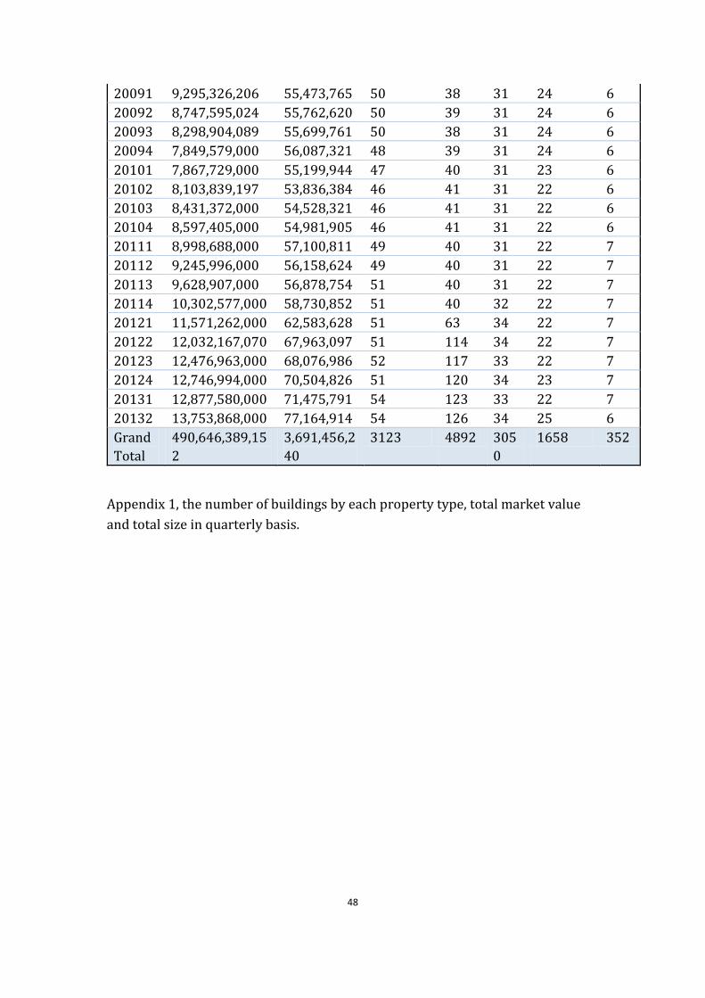
Appendix 1, the number of buildings by each property type, total market value

and total size in quarterly basis.

49

Appendix 2

Code for optimization model in Matlab:

global stats k penalty_equ;

load('timeIndex');

filename = 'Grace_Fu_Thesis_Data_MASKED - Copy2_V2.xlsx';

sheetname = 'NPI_Returns0';

% stats.CFNAI = xlsread(filename,sheetname,'BA2:BA140');

% stats.YYYYQ2 = xlsread(filename,sheetname,'AT2:AT140');

stats.YYYYQ = xlsread(filename,sheetname,'B2:B13128');

stats.Weight = xlsread(filename,sheetname,'AM2:AM13128');

stats.AdjustedCapRate = xlsread(filename,sheetname,'U2:U13128');

stats.SqFt = xlsread(filename,sheetname,'AR2:AR13128');

stats.TotalReturn = xlsread(filename,sheetname,'T2:T13128');

stats.Top6City = xlsread(filename,sheetname,'AH2:AH13128');

stats.Northeast = xlsread(filename,sheetname,'AI2:AI13128');

stats.West = xlsread(filename,sheetname,'AJ2:AJ13128');

stats.Midwest = xlsread(filename,sheetname,'AK2:AK13128');

stats.South = xlsread(filename,sheetname,'AL2:AL13128');

stats.Industrial = xlsread(filename,sheetname,'AC2:AC13128');

stats.Numberofbuilding = xlsread(filename,sheetname,'AP2:AP13128');

stats.timeindex=timeIndex;

% remove bad points

badpoints = find(stats.Weight==0 | stats.SqFt==0);

stats.YYYYQ(badpoints)=[];

stats.Weight(badpoints)=[];

stats.AdjustedCapRate(badpoints)=[];

stats.SqFt(badpoints)=[];

stats.TotalReturn(badpoints)=[];

stats.Top6City(badpoints)=[];

stats.Northeast(badpoints)=[];

stats.West(badpoints)=[];

stats.Midwest(badpoints)=[];

stats.South(badpoints)=[];

stats.Industrial(badpoints)=[];

stats.Numberofbuilding(badpoints)=[];

%% penalize equality constraints

penalty_equ = 0;

50

% %% build timeindex

% timeindex=zeros(138,1);

% timeindex(1)=19784;

% index=2;

% for year=1979:2012

% for quarter=1:4

% timeindex(index) = str2double(strcat(int2str(year),int2str(quarter)));

% index=index+1;

% end

% end

% timeindex(index)=20131;

% timeindex(index+1)=20132;

% clear year index quarter;

%% compute constraint matrix

Z=[];

For i=1:139

indice=find(stats.YYYYQ==stats.timeindex(i));

Z=[Z; ones(size(indice))*stats.CFNAI(i)];

End

Z=Z./stats.Numberofbuilding;

A = -[stats.AdjustedCapRate.*Z stats.SqFt.*Z stats.Industrial.*Z stats.Top6City.*Z

stats.Northeast.*Z stats.West.*Z stats.Midwest.*Z stats.South.*Z];

b = stats.Weight;

% Aeq = [];

% for i=1:139

% indice=find(stats.YYYYQ==stats.timeindex(i));

% At = [mean(stats.AdjustedCapRate(indice)) mean(stats.SqFt(indice))

mean(stats.Top6City(indice)) mean(stats.Industrial(indice))];

% Aeq = [Aeq; At];

% end

% beq=zeros(139,1);

%

options = optimset('Algorithm','interior-point');

k = 2;

a02 = fmincon(@objective,zeros(8,1),A,b,[],[],[],[],[],options)

%

k = 5;

51

a05 =

fmincon(@objective,zeros(8,1),A,b,[],[],[],[],[],options) %,[],[],[],[],[],options

k = 9;

a09 = fmincon(@objective,zeros(8,1),A,b,[],[],[],[],[],options)

functionob=objective(a)

% a = [0 0 0 0]'

global stats k penalty_equ;

ob=0;

for i=1:139

indice=find(stats.YYYYQ==stats.timeindex(i));

wBar= stats.Weight(indice);

N =length(indice);

% stats.CFNAI1 = stats.CFNAI1(2:140);

Z=stats.CFNAI(find(stats.YYYYQ2==stats.timeindex(i)));

r=stats.TotalReturn(indice);

X = [stats.AdjustedCapRate(indice) stats.SqFt(indice) stats.Industrial(indice)

stats.Top6City(indice) stats.Northeast(indice) stats.West(indice)

stats.Midwest(indice) stats.South(indice)];

Rp=(wBar+1/N*X*a*Z)'*r;

% ob=ob+(1+Rp)^(1-k);

% penalize equlity constraint

ob=ob+(1+Rp)^(1-k)/(1-k) - penalty_equ*sum(1/N*X*a*Z)^2;

end

52

References

Do Changes in Illiquidity Affect Investors’ Expectations? An Analysis of the

Commercial Property Returns. Yuichiro Kawaguchi, J. Sa-Aadu, James D. Shilling

(2007)

Stocks are from Mars, Real Estate is from Venus. Arvind Pai and David Gelter.

(2007)

Parametric Portfolio Policies: Exploiting Characteristics in the Cross-Section of

Equity Returns. Michael W. Brandt, Pedro Santa-Clara, Rossen Valkanov (2009)

Expected Returns and Expected Growth in Rents of Commercial Real Estate.

Plazzi, A., Torous, W., & Valkanov, R. (2010). Review of Financial Studies, 23(9),

3469–3519. doi:10.1093/rfs/hhq069

Applying MPT to Institutional Real Estate Portfolios: The Good, the Bad and the

Uncertain. Pagliari, Joseph L. Jr., James R. Webb, and Joseph J. Del Casino. (1995)

Exploiting Property Characteristics in Commercial Real Estate Portfolio

Allocation. Alberto Plazzi, Walter Torous and Rossen Valkanov (2011)

Real Estate is Not Normal: A Fresh Look at Real Estate Return Distributions.

Michael S. Young, Richard A. Graff (1995)

Real Estate Return Correlations: Real-World Limitations on Relationships

Inferred from NCREIF Data. Richard A Graff, Michael S. Young.(1996)

Determining the Current Optimal Allocation to Property: A Study of Australian

Fund Managers. Wejendra Reddy. (2012)

Property-Level Performance Attribution: Demonstrating a Practical Tool for Real

Estate Investment Management Diagnostics. Tony Feng. (2010)

The Vacancy Rate and Rent Levels in the Commercial Office Market. James R.

Frew and G. Donald Jud (1988)

Vacancy, Search and Prices in a Housing Market Matching Model. William C.

Wheaton(1990).

53