October 2000

NASA/TM-2000-210552

Exploratory Studies in GeneralizedPredictive Control for Active AeroelasticControl of Tiltrotor Aircraft

Raymond G. Kvaternik and Jer-Nan JuangLangley Research Center, Hampton, Virginia

Richard L. BennettBell Helicopter Textron, Inc., Fort Worth, Texas

The NASA STI Program Office ... in Profile

Since its founding, NASA has been dedicatedto the advancement of aeronautics and spacescience. The NASA Scientific and TechnicalInformation (STI) Program Office plays a keypart in helping NASA maintain this importantrole.

The NASA STI Program Office is operated byLangley Research Center, the lead center forNASAÕs scientific and technical information.The NASA STI Program Office providesaccess to the NASA STI Database, the largestcollection of aeronautical and space scienceSTI in the world. The Program Office is alsoNASAÕs institutional mechanism fordisseminating the results of its research anddevelopment activities. These results arepublished by NASA in the NASA STI ReportSeries, which includes the following reporttypes:

· TECHNICAL PUBLICATION. Reports

of completed research or a majorsignificant phase of research thatpresent the results of NASA programsand include extensive data or theoreticalanalysis. Includes compilations ofsignificant scientific and technical dataand information deemed to be ofcontinuing reference value. NASAcounterpart of peer-reviewed formalprofessional papers, but having lessstringent limitations on manuscriptlength and extent of graphicpresentations.

· TECHNICAL MEMORANDUM.

Scientific and technical findings that arepreliminary or of specialized interest,e.g., quick release reports, workingpapers, and bibliographies that containminimal annotation. Does not containextensive analysis.

· CONTRACTOR REPORT. Scientific and

technical findings by NASA-sponsoredcontractors and grantees.

· CONFERENCE PUBLICATION.Collected papers from scientific andtechnical conferences, symposia,seminars, or other meetings sponsoredor co-sponsored by NASA.

· SPECIAL PUBLICATION. Scientific,

technical, or historical information fromNASA programs, projects, and missions,often concerned with subjects havingsubstantial public interest.

· TECHNICAL TRANSLATION. English-

language translations of foreignscientific and technical materialpertinent to NASAÕs mission.

Specialized services that complement theSTI Program OfficeÕs diverse offeringsinclude creating custom thesauri, buildingcustomized databases, organizing andpublishing research results ... evenproviding videos.

For more information about the NASA STIProgram Office, see the following:

· Access the NASA STI Program HomePage at http://www.sti.nasa.gov

· E-mail your question via the Internet to

help@sti.nasa.gov · Fax your question to the NASA STI

Help Desk at (301) 621-0134 · Phone the NASA STI Help Desk at

(301) 621-0390 · Write to:

NASA STI Help Desk NASA Center for AeroSpace Information 7121 Standard Drive Hanover, MD 21076-1320

National Aeronautics andSpace Administration

Langley Research CenterHampton, Virginia 23681-2199

October 2000

NASA/TM-2000-210552

Exploratory Studies in GeneralizedPredictive Control for Active AeroelasticControl of Tiltrotor Aircraft

Raymond G. Kvaternik and Jer-Nan JuangLangley Research Center, Hampton, Virginia

Richard L. BennettBell Helicopter Textron, Inc., Fort Worth, Texas

Available from:

NASA Center for AeroSpace Information (CASI) National Technical Information Service (NTIS)7121 Standard Drive 5285 Port Royal RoadHanover, MD 21076-1320 Springfield, VA 22161-2171(301) 621-0390 (703) 605-6000

The use of trademarks or names of manufacturers in this report is for accurate reporting and does not constitute anofficial endorsement, either expressed or implied, of such products or manufacturers by the National Aeronauticsand Space Administration.

This paper was presented at the American Helicopter Society Northeast Region Specialists' Meeting onActive Controls Technology, Bridgeport, CT, October 4-5, 2000. The full paper, which consisted of a setof charts and a text explanation of each chart, is reproduced in this report.

iii

Exploratory Studies in Generalized Predictive Controlfor Active Aeroelastic Control of Tiltrotor Aircraft∗

Raymond G. Kvaternik and Jer-Nan JuangNASA Langley Research Center

Hampton, VA

and

Richard L. BennettBell Helicopter Textron, Inc

Fort Worth, TX

Abstract

The Aeroelasticity Branch (AB) at NASA Langley Research Center has along and substantive history of tiltrotor aeroelastic research. That research hasincluded a broad range of experimental investigations in the Langley TransonicDynamics Tunnel (TDT) using a variety of scale models and the development ofessential analyses. Since 1994, the tiltrotor research program has been using a1/5-scale, semispan aeroelastic model of the V-22 designed and built by BellHelicopter Textron Inc (BHTI) in 1983. That model has been refurbished to forma tiltrotor research testbed called the Wing and Rotor Aeroelastic Test System(WRATS) for use in the TDT. In collaboration with BHTI, studies under thecurrent tiltrotor research program are focused on aeroelastic technology areashaving the potential for enhancing the commercial and military viability oftiltrotor aircraft. Among the areas being addressed, considerable emphasis isbeing directed to the evaluation of modern adaptive multi-input multi-output(MIMO) control techniques for active stability augmentation and vibrationcontrol of tiltrotor aircraft. As part of this investigation, a predictive controltechnique known as Generalized Predictive Control (GPC) is being studied toassess its potential for actively controlling the swashplate of tiltrotor aircraft toenhance aeroelastic stability in both helicopter and airplane modes of flight. Thispaper summarizes the exploratory numerical and experimental studies that wereconducted as part of that investigation.

∗ Presented at the American Helicopter Society Northeast Region Active Controls Technology Conference,Bridgeport, CT, October 4-5, 2000.

1

Exploratory Studies in Generalized Predictive Controlfor Active Aeroelastic Control of Tiltrotor Aircraft

Raymond G. Kvaternik and Jer-Nan Juang

NASA Langley Research Center

and

Richard L. Bennett

Bell Helicopter Textron

Presented at the

American Helicopter Society Northeast RegionActive Controls Technology Conference

Bridgeport, CTOctober 4-5, 2000

Outline

● Introductory remarks

● Theoretical development

● Features characterizing method

● Computational considerations

● Implementation considerations

● Illustrative numerical and experimental results

● Concluding remarks

● Status and plans

2

Some Relevant Background

● AB/TDT has a long history of tiltrotor aeroelastic research

● Research has included a broad range of experimentalinvestigations and the development of essential analyses

● Since 1994, tiltrotor research program has been using a1/5-scale, semispan aeroelastic model of the V-22

● AB/BHTI cooperative study of promising tiltrotoraeroelastic technology areas underway since 1994

● Evaluation of modern adaptive MIMO control techniquesfor active stability augmentation a major activity

● GPC-based method for actively controlling swashplate toenhance stability under investigation since 1997

The Aeroelasticity Branch (AB) at NASA Langley Research Center hasa long and substantive history of tiltrotor aeroelastic research (ref. 1). Thatresearch has included a broad range of experimental investigations in theLangley Transonic Dynamics Tunnel (TDT) using a variety of scale modelsand the development of essential analyses. Since 1994, the tiltrotor researchprogram has been using a 1/5-scale, semispan aeroelastic model of the V-22designed and built by Bell Helicopter Textron Inc (BHTI) in 1983. That modelhas been refurbished to form a tiltrotor research testbed called the Wing andRotor Aeroelastic Test System (WRATS) for use in the TDT. In collaborationwith BHTI, studies under the current tiltrotor research program are focused onaeroelastic technology areas having the potential for enhancing the commercialand military viability of tiltrotor aircraft. Among the areas being addressed,considerable emphasis is being directed to the evaluation of modern adaptivemulti-input multi-output (MIMO) control techniques for active stabilityaugmentation and vibration control of tiltrotor aircraft. As part of thisinvestigation, a predictive control technique known as Generalized PredictiveControl (GPC) is being studied to assess its potential for actively controllingthe swashplate of tiltrotor aircraft to enhance aeroelastic stability in bothhelicopter and airplane modes of flight. This paper summarizes the exploratorynumerical and experimental studies that were conducted as part of thatinvestigation.

3

Approaches to Control

● Conventional control approach– System modeling and verification (off-line)

– Controller design and verification (off-line)

● Adaptive control approach– On-line/real-time system identification

– On-line/real-time controller design

– User specification of model order, horizons, and control weights

● Autonomous control approach– System identification/controller design combined into one step

– Automated estimation of system order and disturbances

– Automated adjustment of control weights and control gains

– All done on-line and in real-time

The approaches to active control may be grouped into three generalcategories: conventional control, adaptive control, and autonomous control.

Conventional approach: Uses an explicit plant model represented by atransfer function or state-space model. Determination and verification of thesystem’s transfer function and the design of the controller are done off-line.LQR, H∞, H2��DQG� �V\QWKHVLV�DUH�H[DPSOHV�RI�VXFK�DSSURDFKHV�

Adaptive approach: The term adaptive as used here refers to a real-timedigital system that updates the system identification (SID) parameters based oninput/output data, uses the updated system parameters to compute a new set ofcontrol parameters, and then computes the next set of commands to be sent tothe actuators, with all computations being done on-line. The user specifies theorder of the system model, the prediction and control horizons, and the controlweights.

Autonomous approach: SID and controller design are combined into onestep. Estimation of system order and disturbances, and adjustment of controlweights and control gains (e.g., via fuzzy logic, neural nets, and geneticalgorithms) are all automated. All computations are done on-line and in real-time. Autonomous control is a very active area of research at this time.

The work addressed in this paper falls into the second category.

4

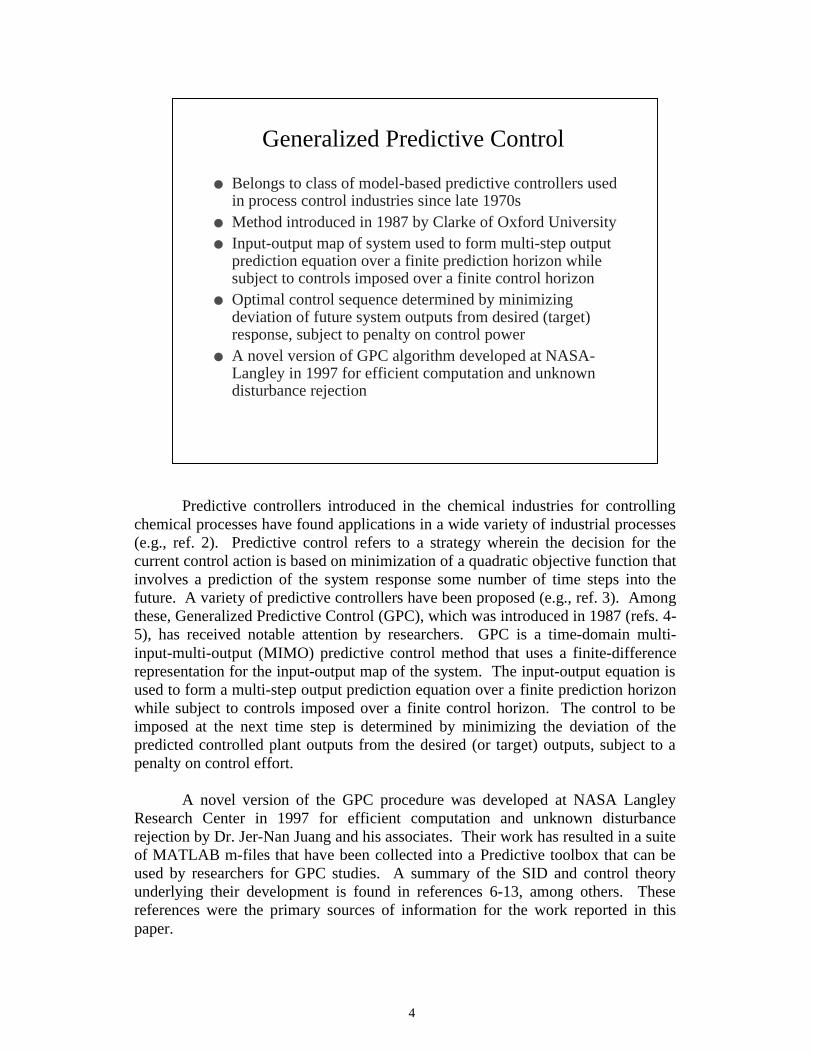
Generalized Predictive Control

● Belongs to class of model-based predictive controllers usedin process control industries since late 1970s

● Method introduced in 1987 by Clarke of Oxford University● Input-output map of system used to form multi-step output

prediction equation over a finite prediction horizon whilesubject to controls imposed over a finite control horizon

● Optimal control sequence determined by minimizingdeviation of future system outputs from desired (target)response, subject to penalty on control power

● A novel version of GPC algorithm developed at NASA-Langley in 1997 for efficient computation and unknowndisturbance rejection

Predictive controllers introduced in the chemical industries for controllingchemical processes have found applications in a wide variety of industrial processes(e.g., ref. 2). Predictive control refers to a strategy wherein the decision for thecurrent control action is based on minimization of a quadratic objective function thatinvolves a prediction of the system response some number of time steps into thefuture. A variety of predictive controllers have been proposed (e.g., ref. 3). Amongthese, Generalized Predictive Control (GPC), which was introduced in 1987 (refs. 4-5), has received notable attention by researchers. GPC is a time-domain multi-input-multi-output (MIMO) predictive control method that uses a finite-differencerepresentation for the input-output map of the system. The input-output equation isused to form a multi-step output prediction equation over a finite prediction horizonwhile subject to controls imposed over a finite control horizon. The control to beimposed at the next time step is determined by minimizing the deviation of thepredicted controlled plant outputs from the desired (or target) outputs, subject to apenalty on control effort.

A novel version of the GPC procedure was developed at NASA LangleyResearch Center in 1997 for efficient computation and unknown disturbancerejection by Dr. Jer-Nan Juang and his associates. Their work has resulted in a suiteof MATLAB m-files that have been collected into a Predictive toolbox that can beused by researchers for GPC studies. A summary of the SID and control theoryunderlying their development is found in references 6-13, among others. Thesereferences were the primary sources of information for the work reported in thispaper.

5

Adaptive Control Process

System Identification&Disturbance Estimation

Predictive Control(Feedback/Feedforward)

Input (u)

Disturbance (d)

Output (y)Plant

uc

uid

The essential features of the adaptive control process used in the presentGPC investigation are depicted in the diagram above. The system (plant) has rcontrol inputs u, m measured outputs y, and is subject to unknown externaldisturbances d. Measurement noise is also present. There are two fundamentalsteps involved: (1) identification of the system; and (2) use of the identifiedmodel to design a controller. A finite-difference model in the form of an Auto-Regressive moving average with eXogenous input (ARX) model is used here.This model is used for both system ID and controller design. Systemidentification is done on-line in the presence of any disturbances acting on thesystem, as indicated in the center box of the diagram. In this way, an estimate ofthe disturbance model is reflected in the identified system model and does nothave to be modeled separately. This approach represents a case of feedback withembedded feedforward. Because the disturbance information is embedded in thefeedforward control parameters, there is no need for measurement of thedisturbance signal (ref. 13). The parameters of the identified model are used tocompute the predictive control law. A random excitation uid (sometimes calleddither) is applied initially with uc equal to zero to identify the open-loop system.Dither is added to the closed-loop control input uc if it is necessary to re-identifythe system while operating in the closed-loop mode.

6

Form of Model and Control Law Equations

● ARX model used for system identification

● Control law equation

y k y k y k y k p

u k u k u k pp

p

( ) =a a ab b b

1 2

0 1

1 2

1

( - ) + ( - ) + + ( - )

+ ( ) + ( - ) + + ( - )

L

L

u k y k y k y k p

u k y k u k p

c c

p

c

c c

p

c

c ( - ) + ( - ) + + ( - )

+ ( - ) + ( - ) + + ( - )

( ) =a a a

b b b1 2

1 2

1 2

1 2

L

L

The relationship between the input and output time histories of a MIMOsystem are described by the time-domain AutoRegressive eXogenous (ARX)finite-difference model shown in the first equation. This equation states that thecurrent output y(k) at time step k may be estimated by using p sets of theprevious output and input measurements, y(k-1),…, y(k-p) and u(k-1),…,u(k-p);and the current input measurement u(k). The integer p is called the order of theARX model. The coefficient matrices i and i appearing in this equation arereferred to as observer Markov parameters (OMP) or ARX parameters and arethe quantities to be determined by the identification algorithm. Closed-looprobustness is enhanced by performing the system identification in the presenceof the external disturbances acting on the system, thereby ensuring thatdisturbance information will be incorporated into the system model. The goal ofSID is to determine the OMP based on input and output data. The OMP may bedetermined by any SID techniques that returns an ARX model of the system.

The ARX model is used to design the controller and leads to a controllaw that in the case of a regulator problem has the general form given by thesecond equation. This equation indicates that the current control input uc(k) maybe computed using p sets of the previous input and output measurements. Thecoefficient matrices and appearing in this equation are the control gainmatrices. The derivation of the parameters appearing in the SID and control lawequations is described below.

a i

cb i

c

7

System Identification

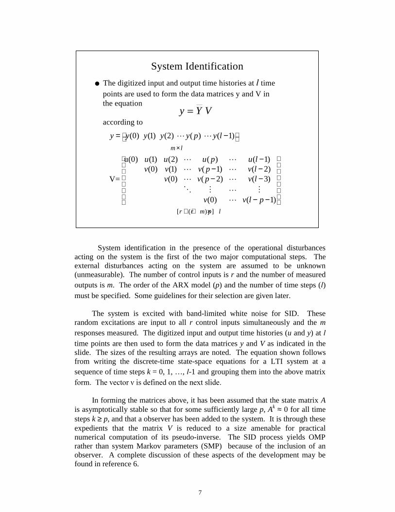
● The digitized input and output time histories at l time points are used to form the data matrices y and V in the equation

according toy Y V=

[ ( ) ]

(0) (1) (2) ( ) ( 1)

u(0) (1) (2) ( ) ( 1)(0) (1) ( 1) ( 2)

(0) ( 2) ( 3)V=

(0) ( 1)

m l

r r m p l

y y y y y p y l

u u u p u lv v v p v l

v v p v l

v v l p

×

+ + ×

= −

−− −− −

− −

L L

L LL LL LO M L M

L

System identification in the presence of the operational disturbancesacting on the system is the first of the two major computational steps. Theexternal disturbances acting on the system are assumed to be unknown(unmeasurable). The number of control inputs is r and the number of measuredoutputs is m. The order of the ARX model (p) and the number of time steps (l)must be specified. Some guidelines for their selection are given later.

The system is excited with band-limited white noise for SID. Theserandom excitations are input to all r control inputs simultaneously and the mresponses measured. The digitized input and output time histories (u and y) at ltime points are then used to form the data matrices y and V as indicated in theslide. The sizes of the resulting arrays are noted. The equation shown followsfrom writing the discrete-time state-space equations for a LTI system at asequence of time steps k = 0, 1, …, l-1 and grouping them into the above matrixIRUP���7KH�YHFWRU� �LV�GHILQHG�RQ�WKH�QH[W�VOLGH�

In forming the matrices above, it has been assumed that the state matrix Ais asymptotically stable so that for some sufficiently large p, Ak ≈ 0 for all timesteps k ≥ p, and that a observer has been added to the system. It is through theseexpedients that the matrix V is reduced to a size amenable for practicalnumerical computation of its pseudo-inverse. The SID process yields OMPrather than system Markov parameters (SMP) because of the inclusion of anobserver. A complete discussion of these aspects of the development may befound in reference 6.

8

The vector �N� that appears in the data matrix V is formed from thevectors u(k) and y(k) as indicated above. Because of the introduction of anobserver into the discrete state equations for the system (ref. 6), the quantities i

and i in are referred to as observer Markov parameters (OMP). Thesolution for , the vector of observer Markov parameters, is obtained by solvingthe equation y = * V for as shown in the bottom equation in the slideabove. If the product VVT is a well-conditioned matrix, the ordinary inverse canbe taken as shown. Otherwise, a pseudo-inverse must be used. It should benoted that because the size of VVT is much smaller than V, a pseudo-inverse maybe appropriate even if the product is well conditioned.

YY

Y

Y

System Identification (Concluded)

● The vector in the matrix is formed according to

● is the matrix of observer Markov parameters (OMP)which are to be identified and has the form

● The solution for is given by

( )v k V

( ) 1

( )( )

( )r m

u kv k

y k

+ ×

=

Y

p0 1 1 2 2 3 3

[ ( ) ]

p

m r m r m m m r m m m r m m m r m m

m r r m p

Y β β α β α β α β α

× × × × × × × × ×× + +

= L

Y-1† y y = T TY V V V V=

where † denotes the pseudo-inverse.

9

Derivation of Multi-Step Output Prediction Equation

The input-output map is given by the ARX equation

y k y k y k y k p

u k u k u k p

p

p

( ) =a a a

b b b1 2

0 1

1 2

1

( - ) + ( - ) + + ( - )

+ ( ) + ( - ) + + ( - )

L

L

Using this equation, the output at time step k+j can be written as

where the coefficient matrices are combinations of αi and βi

( ) ( ) ( )1 2

(1) ( )0 o

( ) (j) ( )1 2

( ) ( -1) + ( -2) + + ( - )

+ ( )+ ( 1) ( )

+ ( -1)+ ( 2) + ( - )

j j jp

jo

j jp

y k j y k y k y k p

u k j u k j u k

u k u k u k p

α α α

β β β

β β β

+ =

+ + − + +

− +

L

L

L

The one-step ahead ARX equation describing the input-output map of thesystem is the starting point for deriving the multi-step output prediction equationthat is needed for designing the MIMO controller. Using the one-step aheadequation shown at the top of the slide, the output at time step k+j may be writtenin the form shown in the second equation, where the coefficient matrices aregiven by recursive expressions involving the matrices i and i appearing in theARX equation (ref. 10). The matrices i and i are determined by the systemidentification process described earlier.

The second equation states that the output y(k+j) at time step k+j may beestimated by using p sets of the previous output and input measurements,y(k-1),…, y(k-p) and u(k-1),…,u(k-p), and the (unknown) current and futureinputs, u(k), u(k+1),…,u(k+j). Letting j range over the set of values j = 1, 2,…, hp-1, the resulting equations can be assembled into a multi-step ahead outputprediction equation having the form indicated in the next slide.

10

Derivation of Prediction Equation (Concluded)

Letting j range over the set of values j = 1, 2, …, q, …, hp-1, the resultingequations can be assembled into the multi-step output prediction equation:

Current &Future Output Past Input

Past OutputCurrent &

Future Input

1 111

( ) ( ) ( ) ( )p c

p c p pcp

h h p ph m x h r h m x pr h m x pm

pr x pm xh r xh m x

y k u k u k p y k p= + − + −W E D

where the coefficient matrices are formed from combinationsof the observer Markov parameters αi and βi appearing in the ARXequation describing the input-output map of the system, and where hp isthe prediction horizon, hc is the control horizon, and hc ö hp.

, ,W E D

GPC is based on system output predictions over a finite horizon hp knownas the prediction horizon. To predict future plant outputs, some assumptionneeds to be made about future control inputs. In determining the future controlinputs for GPC, it is assumed that the control is applied over a finite horizon hc

known as the control horizon. Beyond the control horizon, the control input isassumed to be zero. In GPC, the control horizon is always equal to or less thanthe prediction horizon.

The general form of the multi-step ahead prediction equation indicating thesizes of the constituent matrices is shown in this slide. The coefficient matrices , , and are formed from combinations of the observer Markov parameters

i and i appearing in the ARX equation describing the input-output map of thesystem. The objective is to predict the output for hp time steps ahead, given theinput for hc steps ahead, where hc � hp. The quantity yhp(k) is the vectorcontaining the predicted future outputs, whereas uhc(k) is the vector containingthe future control inputs yet to be determined. The quantities up(k-p) and yp(k-p)are vectors containing the previous p sets of control inputs and outputs,respectively.

W E D

11

The expanded form of the multi-step output prediction equation for thecase in which the control horizon is less than the prediction horizon is shown inthis slide. The OMP i and i determined in system identification form the firstblock rows of the coefficient matrices , , and in the equation. The termsin the remaining rows are computed using the recursive relations indicated in theboxes (ref. 10). All terms in the above equation are known, except for the hc

sets of future commands, and the hp sets of predicted responses. The goal of theGPC control algorithm is to determine the set of future commands u(k), u(k+1),…, u(k+hc-1) that are required to achieve a desired predicted response y(k),y(k+1), …, y(k+hp-1).

It should be remarked that the system Markov parameters (SMP), whichare commonly used as the basis for identifying discrete-time models for lineardynamical systems, form the first block column in the matrix ; the remainingblock columns are formed from subsets of the SMP. The Markov parametersare the pulse response of a system and are unique for a given system. Thediscrete-time state-space matrices A, B, C, and D are embedded in the SMP.

The multi-step output prediction equation is used to define an objectivefunction whose minimization with respect to uhc(k) leads to the control law fromwhich a vector of future control inputs can be computed using the p sets ofprevious control inputs and measured outputs.

W D E

W

(1)

( 1)

( )

( 1)

( 2)

( 1) (1)

( 2

1

) (

2

)

( )

( 1)( )

( 1)( 1)

( )( 1)

( 1) p pp c

o

qo

qo

h

o

o

qo o

qo o

c

h h hp o

o

p

o

y k

y ku k

u ky k q

y k qu k h

y k h

β

β ββ β

β

β

α α α

β

ββ

ββ

−

−

−

−

− −

−

+ + + − =

+ + − + −

+

M M OM

LM

L

M M O MM

L

L

(1) (1) (1) (1)1 2 1

( 1) ( 1) ( 1) ( 1)1 2 1

( ) ( ) ( ) ( )1 2 1

( 1) ( 1) ( 1) ( 1)1 2

1 2

1

1

( 1)

( 2)

( 1)

( )p p p p

p p

q q q qp p

q q q qp p

h h h h

p p

p

y k

y k

y k p

y k p

α α α α

α α α αα α α α

α α α

α

α

β β

−

− − − −−

−

− − − −−

−

− + − +

−

L

L

M M O M M

L M

L

M M O M M

K

(1) (1) (1) (1)1 2 1

( 1) ( 1) ( 1) ( 1)1 2

( ) ( ) ( ) ( )1 2 1

( 1) ( 1) ( 1) ( 1)1 2

1

1

( 1)

( 2)

( 1)

( )p p p p

p p

q q q qp p

q q q qp p

h h

p

p p

p

h h

u k

u k

u k p

u k p

β β β β

β β β ββ β β β

β β β β

β β

−

− − − −

−

− − − −−

− −

− − +

−

L

M M O M M

L M

L

M M O M M

K

Expanded Form of Multi-Step Output Prediction Equation

1)1(

1)1()(

1 −−−

− += pqq

pq

p αααα

0)1(

1)1(

1)(

0 βαββ −− += qqq

1)1(

1)1()(

1 −−−

− += pqq

pq

p βαββ

h hc p<

12

Derivation of Control Law

c c

TTh hJ R Qu uε ε= +

Define an error function :

( ) ( ) ( ) ( ) ( ) ( )T T pp c ph hk k k k k p k py y y u u yε = − = − − − − −W E D

Define an objective function J:

Minimize J with respect to :

( )†

1

( ) ( ) ( ) ( ) ( )

C

c

T TT p ph

h r

k R Q R y k u k p y k pu×

= − + − + − + −W W W E D

Retain the first component (first r rows) of :

1( ) ( ) ( ) ( )T p p

c c cc

rk y k u k p y k pu γ β α

×= − + − + −

( )chu k

( )chu k

The predictive control law is obtained by minimizing the deviation of thepredicted controlled response (as computed from the multi-step outputprediction equation) from a specified target response over a prediction horizonhp. To this end, one first defines an error function that is the difference betweenthe desired (target) response yT (k) and the predicted response yhp(k) and formsan objective function J quadratic in the error and the unknown future controls.Two weighting matrices are included in the objective function: Q (symmetricand positive-definite ) is used to limit the control effort and stabilize the closed-loop system; R (symmetric and positive-semidefinite) is used to weight therelative importance of the differences between the target and predictedresponses. Typically, Q and R are assumed to be diagonal and for Q to have thesame value wc along its diagonal and R to have the same value wr along itsdiagonal. Minimizing J with respect to uhc(k) and solving for uhc(k) gives thecontrol sequence to be applied to the system over the next hc time steps. Thefirst r values (corresponding to the first future time step) are applied to the rcontrol inputs, the remainder are discarded, and a new control sequence iscalculated at the next time step.

The target response is zero for a regulator problem and non-zero for atracking problem. Q must be tuned to ensure a stable closed-loop system.Typically, hc is chosen equal to hp. However, hc may be chosen less than hp

resulting in a more stable and sluggish regulator.

13

Features Characterizing Method

● Predictive controllers employ a strategy wherein currentcontrol actions are based on prediction of system responseat a number of time steps into the future

● Approach allows one to work directly with an input-output(ARX) model of the system

● SID process employs an observer to enable numericalcomputation of pseudo-inverse for calculation of OMP

● Controller is thus inherently observer-based but no explicitconsideration of its presence needs to be taken into account

● System identification is performed in the presence of anydisturbances acting on system

Predictive controllers such as GPC employ a strategy wherein the values ofthe current control inputs are based on the predicted responses at a number oftime steps into the future. Such an approach lends itself to the use of an ARXmodel to represent the system for both system identification and controllerdesign. The SID process used makes recourse to an observer to enablenumerical computation of the pseudo-inverse needed for calculation of the OMPthat comprise the coefficients of the ARX equation. The controller is thusinherently observer-based but no explicit consideration of the observer needs tobe taken into account in the implementation.

In practice, the disturbances acting on the system are unknown orunmeasurable. However, as discussed in reference 13, by performing the SID inthe presence of the external disturbances acting on a system, a disturbancemodel is implicitly incorporated into the identified observer Markov parameters.However, the identified model must be larger than the true system model toaccommodate the unknown disturbances.

14

Features Characterizing Method (Continued)

● Disturbance model is implicitly incorporated into theidentified coefficients (OMP) of the ARX model

● Effects of unknown disturbances embedded in coefficientmatrices and (and hence and ) because SIDdone with disturbances acting on system

● Estimated order of ARX model used for system ID givenby

● Prediction and control horizons are set according to

cα cβ

p ceiln n

msystem states disturbance states�

+���

���

D E

h p h hp c p� �

The disturbance model is implicitly incorporated into the identifiedcoefficients (OMP) of the ARX model. Thus, the effects of the unknowndisturbances acting on the system are embedded in the matrices and , andhence the control law matrices c and c.

An expression for estimating the order of the ARX model that is to be usedfor SID is given in the slide. The number of system states is typically chosen tobe twice the number of significant structural modes; the number of disturbancestates is set to twice the number of frequencies in the disturbance; m is thenumber of output measurements. If measurement noise is of concern, the orderof p so computed should be increased to allow for computational poles and zerosto improve system identification in the presence of noise. In practice, simplychoosing p to be 5-6 times the number of significant modes in the system isoften adequate.

The prediction and control horizons are set according to the relationsindicated at the bottom of the slide. Although hp can be set equal to p, hp istypically set greater than p to help limit control effort so as not to saturate thecontrol actuators. If the control horizon is greater than the system order aminimum energy (minimum norm) solution is obtained wherein the commandedoutput is shared so that the control actuators don’t fight each other. If hp is setequal to p one obtains a so-called deadbeat controller (ref. 10).

D E

15

Features Characterizing Method (Concluded)

● Extending hc and hp (and hence p) to very large values,GPC solution approaches LQR solution; hence GPCapproximates an optimal controller for large p

● Matrices Q and R are control effort and tracking errorweighting matrices

● Matrix (and hence ) is invariant if system does notchange because it is formed from SMP (which are unique)

● Solution for obtained by an efficient computationalprocedure

W cγ

Y

By extending the prediction and control horizons (and hence p, the order ofthe ARX model) to very large values, the GPC solution approaches that of thelinear quadratic regulator (LQR). Thus, GPC approximates an optimalcontroller for large p (ref. 5).

Weighting matrices Q and R are used to limit the control effort and toweight the relative importance of the differences between the target andpredicted responses, respectively. As mentioned earlier, Q and R are usuallyassumed to be diagonal and for Q to have the same value wc along its diagonaland R to have the same value wr along its diagonal. The GPC solution offers noguarantee of stability and the control weight must be tuned to produce anacceptable solution without going unstable. Reducing wc increases controlauthority and performance but eventually drives the system unstable.

If only the disturbances acting on the system change, there is no need torecalculate (and hence c ) because it is formed solely from the SMP, whichare unique for a given system (ref. 13).

The solution for described earlier involves forming the matrix productsyVT and VVT. Here, these products are obtained using the computationallyefficient procedure described in reference 8.

W

Y

16

GPC Computational Considerations

● System ID in presence of external disturbances for implicitinclusion of disturbance model

● Pseudo-inverse based on SVD techniques

● Basis for recalculation of matrices

● On-line/real-time versus on-line/near-real-time

● Batch versus recursive calculation of OMP

● Efficient computational algorithms and coding

Several considerations dealing with computations should be kept in mindwhen developing algorithms for GPC applications.

SID should be done with the external disturbances acting on the systemso that information about the disturbances is embedded in the OMP. However,depending on the nature of the external disturbances, it may be possible toperform a SID on an undisturbed system and still determine a control law thatresults in satisfactory closed-loop performance.

The computation of pseudo-inverses should be performed using SingularValue Decomposition (SVD) because of the latter’s ability to deal with matricesthat are numerically ill-conditioned. The use of pseudo-inverses (via SVD) isrecommended even in cases where the ordinary inverse may seem appropriate(such as in the operation (VVT)-1 indicated in the expression for the OMP).

The basis for recalculation of matrices needs to be selected. For example,should the system be re-identified and the control law matrices recalculated inevery sampling period, every specified number of time steps (block updating),or only if some event requiring a re-ID occurs? Should all calculations be donein real time, or can some be done in near real time? Should updating of theOMP be done in batch mode or recursively?

Microprocessor speeds are such that it is now often possible to completethe full cycle of GPC computations and apply the commands to the actuatorswithin one sampling period. However, the need for efficient computationalalgorithms and attendant coding is not expected to diminish.

17

GPC Implementation Considerations

● Low-pass filtering of measured time histories

● Cut-off frequency of filter set to Nyquist frequency fN

● Nyquist frequency chosen so that maximum frequency ofinterest is about 75% of fN

● Sampling frequency selected to be between 2-3 times fN

● Length of data stream for SID determined by need for 5-10cycles of lowest frequency mode in measured responses

● Scaling (normalization) of digitized input and output data

● Distribution of computing tasks among computers/CPUs

● Extent of user interaction/involvement

● Constraints on acceptable values of input and output

Several considerations must be taken into account when actuallyimplementing GPC algorithms in hardware for active controls work.

The measured response time histories must be passed through a low-passfilter with a cut-off frequency fc set equal to the Nyquist frequency fN. The latteris chosen so that the maximum frequency of interest is about 75% of fN. Thesampling frequency fS should be at least twice fN to prevent aliasing. However, iffS is made too large the low frequency modes will be poorly identified due to aloss of frequency resolution. A sampling rate between 2 to 3 times fN isgenerally sufficient. Once the sampling frequency has been selected, theminimum number of data points that should be used for SID follows from therequirement of having 5-10 cycles of the lowest frequency mode in the measuredresponse time histories.

Normalization of the input and output data that is used for SID on themaximum actual or expected values of the data is often helpful numerically. Theprocedure will depend on whether the computations are being done in batch modeor recursively.

The computing tasks can be distributed among computers or different CPUson a single computer. The choice will influence the extent of user involvement.

The values of the input and output data that are being used during closed-loop operations must be carefully monitored to ensure that they fall withinacceptable bounds. This is easily done using IF/THEN-type checks in the code.

18

A variety of numerical and experimental studies comprised theexploratory evaluation phase of the GPC investigation during the period 1997-1999. These studies included: (1) Numerical simulations using 3- and 9-DOFmass-spring-dashpot systems varying the number and location of externaldisturbances, the number and location of control inputs, and the number,location, and type of response measurements (displacement, acceleration); (2)Extensive experimental simulations using the BHTI Cobra stick model in whichthe number and location of the shakers used for control and disturbance werevaried; (3) Preliminary assessment of GPC for simulated tracking response usingan XV-15 math model determined using BHTI’s COPTER (COmprehensiveProgram for Theoretical Evaluation of Rotorcraft) flight simulation program(ref. 14); (4) A hover test (April 1998) of a stiff-inplane rotor on the WRATStestbed to explore the vibration reduction capability of GPC (excitation causedby rotor downwash and rpm near resonance); and (5) Ground resonance test(Oct. 1999) of a soft-inplane rotor on the WRATS testbed.

Illustrative Numerical and Experimental Results

● Simulations using lumped-mass-spring-dashpot systems

● Experimental dynamic studies using Cobra stick model

● Simulated tracking control of XV-15 in roll maneuver

● Hover test of stiff-inplane rotor on WRATS

● Ground resonance test of soft-inplane rotor on WRATS

19

The 3-DOF mass-spring-dashpot system used in the 3-DOF simulations isdepicted at the top of the slide.

The masses were equal to 1.0 and the spring rates were all equal to 1000lb/in. The damping coefficients of dashpots 1 and 2 were equal to 0.1 lb/in/sec,but the damping of dashpot 3 was set to – 0.1 lb/in/sec to make the systemunstable (one pair of complex conjugate eigenvalues had a positive real part).

Control was imposed at masses 1 and 3 (r = 2). Accelerations weremeasured at masses 1 and 2 (m = 2). Sinusoidal disturbances were applied atmasses 1 and 2 at a frequency f = 6.276 Hz, which coincided with a naturalfrequency of the system. The expressions used to represent the disturbances inthe simulation are ud1 = 2*cos(2*pi*f*t) and ud2 = 1*sin(2*pi*f*t) and areshown in the plot at the lower left. Also, Ðt = 0.05 sec, l = 300, and p = 5.

The oscillatory diverging behavior of the open-loop system is shown in theplot at the upper right, which shows the time history of the accelerationresponses of masses 1 and 2. The loop was closed after 100 time steps. Thetime histories of the closed-loop responses and control commands are shown inthe plots in the lower right and upper left, respectively.

20

In parallel with the extensive numerical simulations that were beingconducted using the 3- and 9-DOF mass-spring-dashpot systems, bench testswere conducted by Bell Helicopter using the “Cobra stick model” shown in theslide. This model is a 36-inch long, 50-lb, multiple degree-of-freedom lumped-mass dynamic model that approximates the dynamics of a Cobra helicopter.The dominant vertical bending modes of the model have natural frequencies ofabout 8 and 23 Hz. Electromagnetic shakers were used in various combinationsfor imposing external periodic and random disturbances, random excitationsneeded for system identification, and the control inputs called for by the GPCalgorithm.

Cobra Stick Model

External disturbance shaker

Control shakers

21

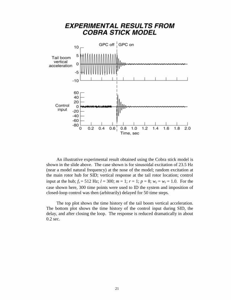
An illustrative experimental result obtained using the Cobra stick model isshown in the slide above. The case shown is for sinusoidal excitation of 23.5 Hz(near a model natural frequency) at the nose of the model; random excitation atthe main rotor hub for SID; vertical response at the tail rotor location; controlinput at the hub; fs = 512 Hz; l = 300; m = 1; r = 1; p = 8; wc = wr = 1.0. For thecase shown here, 300 time points were used to ID the system and imposition ofclosed-loop control was then (arbitrarily) delayed for 50 time steps.

The top plot shows the time history of the tail boom vertical acceleration.The bottom plot shows the time history of the control input during SID, thedelay, and after closing the loop. The response is reduced dramatically in about0.2 sec.

22

A cursory examination of using the GPC algorithm as a means foractuating the controls necessary to execute a prescribed maneuver was made.The subject aircraft was the XV-15 cruising at 150 kts in the airplane mode offlight. The controls considered were collective pitch, longitudinal and lateralcyclic pitch, and pedal. Responses of interest were aircraft pitch, roll, sideslip,and forward velocity. Bell Helicopter’s COPTER flight simulation program(ref. 14) was used to compute the linearized mass, damping, and stiffnessmatrices for a trimmed fight condition as well as components for the B matrix.MATLAB was used to form the A, B, C, and D state matrices and generate thesimulated input-output time histories needed for SID and GPC. A one-cyclesaw-tooth-type roll maneuver was prescribed to be the target response, yT.

Simulated Tracking Control of XV-15 Tiltrotor

● Aircraft in airplane mode of flight;150 kts airspeed; sea level

● Control inputs: Collective, pedal,longitudinal & lateral cyclic pitch,

● Responses: Pitch, roll, sideslip,and forward velocity

● COPTER used to generate linearized mass, damping, and stiffnessmatrices for trimmed flight condition and components for B matrix

● MATLAB used to form A, B, C, and D state matrices and generatesimulated input-output time history needed for SID/GPC

● Roll maneuver prescribed

23

One cycle of a saw-tooth-type roll maneuver was prescribed to be thetarget response, yT. The time histories of this desired response and the actualroll response produced by GPC are shown for comparison at the bottom of theslide. The remaining three responses (pitch, sideslip, and forward velocity) hadnegligible magnitudes and are not plotted.

The time histories of the rudder and lateral cyclic control inputs called forby the GPC algorithm to perform the prescribed roll maneuver are shown at thetop of the slide. The remaining control inputs (collective pitch and longitudinalcyclic pitch) had negligible magnitudes and are not plotted.

The primary structural natural frequencies of the aircraft lie between 0.8and 10 Hz. The values of pertinent GPC parameters are: wc = 1.0, p = 8, hp = hc

= 2p, l = 400, Ðt = .025 sec, fs = 40 Hz.

24

WRATS Model in Aeroelasticity BranchRotorcraft Hover Test Facility

The initial evaluation of GPC on the WRATS testbed was conducted inApril 1998 during a one-week hover dynamics test conducted in the ABrotorcraft hover test facility located in a building adjacent to the TDT. A stiff-inplane gimballed rotor was employed in this investigation. The model is shownabove with its rotor blades removed and replaced by equivalent lumped weightsfor a ground vibration test that was conducted prior to the test. Emphasis in thisinitial evaluation of GPC was on active control of vibration using only thecollective control. To provide a rigorous test of the GPC algorithm, the open-loop response of the model was exaggerated by running the rotor at an rpm thatnearly coincided with the natural frequency of the wing vertical bending mode.Additional excitation of the wing was provided by the downwash associatedwith running the rotor at a high thrust level.

25

Implementation of GPC Algorithm forWRATS Hover Dynamics Test

Identify system parametersCompute αc and βc

Dual-computer approach with user interaction:

Computer #1

Computer #2

User sends αc and βc

to first computer

User sends data tosecond computer

Compute uc using the p latestI/O data sets

(Continuous calculation)

Collect necessary I/O data (on user command)

User selects l, p, hc, hp, wc, wr

For the hover dynamics investigation, the GPC computations weredistributed between two computers and user interaction was required to transferthe data from one computer to the other. On user command, data required forsystem identification was collected on computer #1 and sent to computer #2where SID was performed and the control gain matrices c and c werecomputed. On user command the control parameters were sent to computer #1which used the p latest data sets to (continuously) compute the controlcommands that were sent to the swashplate actuators. If re-identification of thesystem was required, the process was repeated on user command.

All computations were done using MATLAB on PCs with 500 MHzCPUs.

26

Some experimental results obtained during the WRATS hover dynamicstest that illustrate the effectiveness of GPC in reducing rotor-induced vibrationsare shown in this slide, which shows the measured time histories of the open- andclosed-loop responses of the vertical bending moment rear the root of the wing. Itis seen that the response is dramatically reduced within a second after the controlis turned on.

27

Implementation of GPC Algorithm forWRATS Ground Resonance Test

Initialize αc and βc

Collect necessary I/O data(on user command)

Compute uc using the p latestI/O data sets

(Continuous calculation)

Identify system parametersUpdate αc and βc

Single-computer/dual-processor approach:

CPU #1

CPU #2

User selects l, p, hc, hp, wc, wr

For the ground resonance investigation, the GPC computations weredistributed between two CPUs on a single computer with no user interactionrequired for data transfer as in the earlier hover test. On user command, datarequired for system identification was collected on CPU #1 and sent to CPU #2where SID was performed and the control gain matrices c and c werecomputed. The control parameters were automatically sent to CPU #1 whichused the p latest data sets to (continuously) compute the control commands to besent to the swashplate actuators. If re-identification was required, the processwas repeated on user command.

All the algorithms were implemented in dSPACE software on a PC with500 MHz CPUs.

28

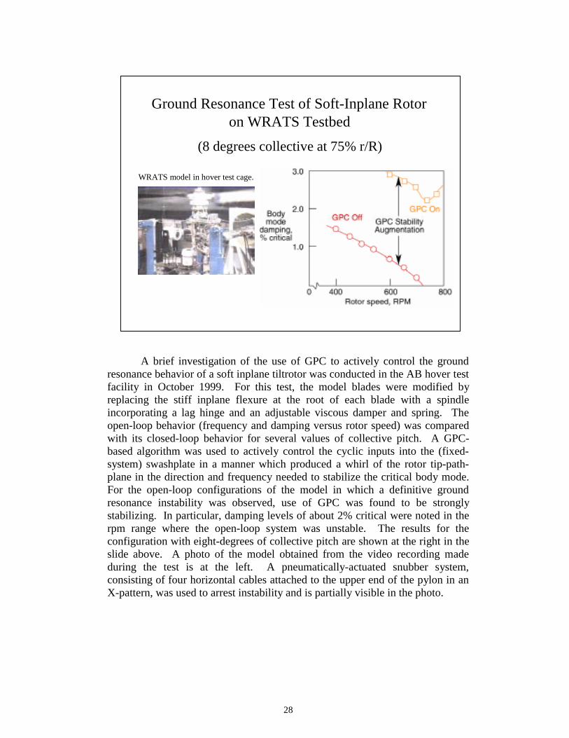
A brief investigation of the use of GPC to actively control the groundresonance behavior of a soft inplane tiltrotor was conducted in the AB hover testfacility in October 1999. For this test, the model blades were modified byreplacing the stiff inplane flexure at the root of each blade with a spindleincorporating a lag hinge and an adjustable viscous damper and spring. Theopen-loop behavior (frequency and damping versus rotor speed) was comparedwith its closed-loop behavior for several values of collective pitch. A GPC-based algorithm was used to actively control the cyclic inputs into the (fixed-system) swashplate in a manner which produced a whirl of the rotor tip-path-plane in the direction and frequency needed to stabilize the critical body mode.For the open-loop configurations of the model in which a definitive groundresonance instability was observed, use of GPC was found to be stronglystabilizing. In particular, damping levels of about 2% critical were noted in therpm range where the open-loop system was unstable. The results for theconfiguration with eight-degrees of collective pitch are shown at the right in theslide above. A photo of the model obtained from the video recording madeduring the test is at the left. A pneumatically-actuated snubber system,consisting of four horizontal cables attached to the upper end of the pylon in anX-pattern, was used to arrest instability and is partially visible in the photo.

WRATS model in hover test cage.

(8 degrees collective at 75% r/R)

Ground Resonance Test of Soft-Inplane Rotoron WRATS Testbed

29

Concluding Remarks

● Exploratory studies of GPC for active aeroelastic controlof tiltrotor aircraft completed

● Studies included numerical simulations and experimentalinvestigations

● GPC-based MIMO active control system was highlyeffective in increasing stability and reducing response

● GPC appears to be a viable approach for active stabilityaugmentation and vibration control of tiltrotor aircraft

● Wind-tunnel tests of WRATS model with GPC needed tomore fully evaluate method

Exploratory numerical and experimental studies into the use of GPC foractive aeroelastic control of tiltrotor aircraft have been completed. A GPC-based MIMO active control system was demonstrated to be be highly effectivein increasing ground resonance stability and reducing vibratory response. Whilethese results are quite encouraging with respect to establishing the viability ofthe method, it is recognized that a broader evaluation of the methodology isneeded to validate GPC-based algorithms for active stability augmentation andvibration control of tiltrotor aircraft.

30

Status and Plans

● Initial wind-tunnel evaluation of GPC on WRATS forairplane-mode stability augmentation completed

● Method highly effective in increasing stability (damping)of critical wing mode

● Continue development and evaluation of GPC-basedmethod for active aeroelastic control

● Improve suite of computational algorithms

● Establish robustness to system nonlinearities

● Conduct additional ground and wind-tunnel tests

The initial wind-tunnel evaluation of GPC on the WRATS testbed forairplane mode stability augmentation has recently (April 2000) been completed.The method was highly effective in increasing stability (damping) of the criticalwing mode for all of the model conditions tested.

Plans are to continue development and evaluation of GPC for activeaeroelastic control. Emphasis will be on improving the suite of computationalalgorithms comprising the current GPC software system developed for WRATS.In this regard, work is underway on providing for the calculation of the closed-loop eigenvalues using closed-loop input-output data and for the recursivecalculation of the OMP.

It is expected that work will also be initiated to establish the robustness ofGPC-based methods to system nonlinearities. Both numerical simulations andexperimental studies are anticipated.

Additional ground and wind tunnel tests are to be conducted as necessaryto evaluate the GPC-based methodology over a broader range of simulated flightand operating conditions.

31

References 1. Yeager, W. T., Jr.; and Kvaternik, R. G.: Contributions of the Langley Transonic

Dynamics Tunnel to Rotorcraft Technology and Development. Presented at the AIAADynamics Specialists Conference, April 5-6, 2000, Atlanta, GA (AIAA Paper 2000-1771).

2. Richalet, J.; Rault, A.; Testud, J. L.; and Papon, J.: Model Predictive Heuristic Control:Applications to Industrial Processes. Automatica, Vol. 14, 1978, pp. 413-428.

3. Clark, D. W. (Ed): Advances in Model-Based Predictive Control. Oxford UniversityPress, New York, 1994.

4. Clark, D. W.; Mohtadi, C.; and Tuffs, P. S.: Generalized Predictive Control, Part 1.The Basic Algorithm, Automatica, Vol. 23, No. 2, 1987, pp. 137-148.

5. Clark, D. W.; Mohtadi, C.; and Tuffs, P. S.: Generalized Predictive Control, Part 2.Extensions and Interpretations, Automatica, Vol. 23, No. 2, 1987, pp. 149-160.

6. Juang, J.-N., Applied System Identification, Prentice Hall, Inc., Englewood Cliffs, New Jersey 07632, 1994, ISBN 0-13-079211-X.

7. Eure, K.W.; and Juang, J.-N.: Broadband Noise Control Using Predictive Techniques.NASA Technical Memorandum 110320, January 1997.

References (Concluded)

8. Juang, J.-N.: State-Space System Realization With Input- and Output-Data Correlation. NASA TP 3622, April 1997.

9 .Juang, J.-N.; and Phan, M. Q.: Recursive Deadbeat Controller Design. NASA TM 112863, May 1997 (also, Journal of Guidance, Control, and Dynamics, Vol. 21, No. 5, Sept.-Oct. 1998, pp. 747-753).

10. Juang, J.-N.; and Phan, M. Q.: Deadbeat Predictive Controllers. NASA TM 112862, May 1997.

11. Eure, K. W.: Adaptive Predictive Feedback Techniques for Vibration Control. Ph.D. Dissertation, Virginia Polytechnic Institute and State University, May 1998.

12. Phan, M. Q.; and Juang, J.-N.: Predictive Controllers for Feedback Stabilization. Journal of Guidance, Control, and Dynamics, Vol. 21, No. 5, Sept.-Oct. 1998, pp. 747-753.

13. Juang, J.-N.; and Eure, K. W.: Predictive Feedback and Feedforward Control for Systems with Unknown Disturbances. NASA/TM-1998-208744, December 1998.

14. Yen, J.; Corrigan, J.; Schillings, J.; and Hsieh, P.: Comprehensive Analysis Methodology at Bell Helicopter: COPTER, presented at the American Helicopter Society Aeromechanics Specialists Conference, San Francisco, CA, Jan. 1994.

REPORT DOCUMENTATION PAGE Form ApprovedOMB No. 0704-0188

Public reporting burden for this collection of information is estimated to average 1 hour per response, including the time for reviewing instructions, searching existing datasources, gathering and maintaining the data needed, and completing and reviewing the collection of information. Send comments regarding this burden estimate or any otheraspect of this collection of information, including suggestions for reducing this burden, to Washington Headquarters Services, Directorate for Information Operations andReports, 1215 Jefferson Davis Highway, Suite 1204, Arlington, VA 22202-4302, and to the Office of Management and Budget, Paperwork Reduction Project (0704-0188),Washington, DC 20503.

1. AGENCY USE ONLY (Leave blank) 2. REPORT DATE October 2000

3. REPORT TYPE AND DATES COVERED Technical Memorandum

4. TITLE AND SUBTITLEExploratory Studies in Generalized Predictive Control for ActiveAeroelastic Control of Tiltrotor Aircraft

5. FUNDING NUMBERS

WU 581-10-11-03

6. AUTHOR(S)Raymond G. Kvaternik, Jer-Nan Juang, and Richard L. Bennett

7. PERFORMING ORGANIZATION NAME(S) AND ADDRESS(ES)

NASA Langley Research CenterHampton, VA 23681-2199

8. PERFORMING ORGANIZATIONREPORT NUMBER

L-18031

9. SPONSORING/MONITORING AGENCY NAME(S) AND ADDRESS(ES)

National Aeronautics and Space AdministrationWashington, DC 20546-0001

10. SPONSORING/MONITORINGAGENCY REPORT NUMBER

NASA/TM-2000-210552

11. SUPPLEMENTARY NOTES Kvaternik and Juang: Langley Research Center; Bennett: Bell Helicopter Textron, Inc. Presented at the American Helicopter Society (Northeast Region) Active Controls Technology Conference, Bridgeport, CT, October 4-5, 2000.12a. DISTRIBUTION/AVAILABILITY STATEMENT

Unclassified-UnlimitedSubject Category 05 Distribution: NonstandardAvailability: NASA CASI (301) 621-0390

12b. DISTRIBUTION CODE

13. ABSTRACT (Maximum 200 words)The Aeroelasticity Branch at NASA Langley Research Center has a long and substantive history of tiltrotor

aeroelastic research. That research has included a broad range of experimental investigations in the LangleyTransonic Dynamics Tunnel (TDT) using a variety of scale models and the development of essential analyses.Since 1994, the tiltrotor research program has been using a 1/5-scale, semispan aeroelastic model of the V-22designed and built by Bell Helicopter Textron Inc. (BHTI) in 1981. That model has been refurbished to form atiltrotor research testbed called the Wing and Rotor Aeroelastic Test System (WRATS) for use in the TDT. Incollaboration with BHTI, studies under the current tiltrotor research program are focused on aeroelastic technologyareas having the potential for enhancing the commercial and military viability of tiltrotor aircraft. Among the areasbeing addressed, considerable emphasis is being directed to the evaluation of modern adaptive multi-input multi-output (MIMO) control techniques for active stability augmentation and vibration control of tiltrotor aircraft. Aspart of this investigation, a predictive control technique known as Generalized Predictive Control (GPC) is beingstudied to assess its potential for actively controlling the swashplate of tiltrotor aircraft to enhance aeroelasticstability in both helicopter and airplane modes of flight. This paper summarizes the exploratory numerical andexperimental studies that were conducted as part of that investigation.14. SUBJECT TERMS

Tiltrotor aeroelasticity; active control; active stability augmentation; active vibrationreduction; generalized predictive control

15. NUMBER OF PAGES 37

16. PRICE CODE A03

17. SEC U RITY CL ASSIF IC AT ION O F REPO R T Unclassified

18. SEC U RITY CL ASSIF IC AT ION O F TH IS PA GE Unclassified

19. SECURITY CLASSIFICATION OF ABSTRACT Unclassified

20. LIMITATION OF ABSTRACT UL

NSN 7540-01-280-5500 Standard Form 298 (Rev. 2-89) Prescribed by ANSI Std. Z-39-18

298-102