Robotics: Science and Systems 2013Berlin, Germany, June 24-28, 2013

1

Exploiting Urban Scenes forVision-aided Inertial Navigation

Dimitrios G. Kottas and Stergios I. RoumeliotisDepartment of Computer Science and Engineering

University of Minnesota, Minneapolis, MNdkottas|stergios at cs.umn.edu.

Abstract—This paper addresses the problem of visual-inertialnavigation when processing camera observations of both pointand line features detected within a Manhattan world. First,we prove that the observations of: (i) a single point, and (ii)a single line of known direction perpendicular to gravity (e.g.,a non-vertical structural line of a building), provide sufficientinformation for rendering all degrees of freedom of a vision-aided inertial navigation system (VINS) observable, up to globaltranslations. Next, we examine the observability properties of thelinearized system employed by an extended Kalman filter (EKF)for processing line observations of known direction, and show thatthe rank of the corresponding observability matrix erroneouslyincreases. To address this problem, we introduce an elegantmodification which enforces that the linearized EKF system hasthe correct number of unobservable directions, thus improvingits consistency. Finally, we validate our findings experimentallyin urban scenes and demonstrate the superior performance ofthe proposed VINS over alternative approaches.

I. INTRODUCTION AND RELATED WORK

Current approaches for estimating the position and attitudeof a vehicle navigating in 3D rely on inertial measurementunits (IMUs) that provide rotational velocity and linear ac-celeration measurements. However, when using commercial-grade IMUs, the integration of the noise and bias in the inertialmeasurements renders the resulting estimates unreliable evenafter a short period of time. For this reason, most inertialnavigation systems (INSs) often rely on GPS to provideperiodic corrections in what is known as GPS-aided INS. Inmany cases (e.g., indoors or within urban canyons), however,the GPS signals are either unavailable or unreliable and thusalternative means for aiding INS are necessary. Vision-aidedINS (VINS) employs cameras to extract motion (and oftenstructure) information from images of the surroundings of theIMU-camera pair, necessary for providing periodic correctionsto the inertial estimates. Recent advances in VINS have led tosuccessful applications to ground [14, 7], aerial [20, 19], andspace exploration [15] vehicles.

Most work to date on VINS has focused on point featuresthat are tracked through sequences of images, or re-detectedwhen returning to the same location. Point features can befound in most natural and man-made environments, and asshown in [7, 10, 8], they provide sufficient information forestimating all degrees of freedom (d.o.f.) of a VINS, except

This work was supported by the University of Minnesota through the DigitalTechnology Center (DTC) and AFOSR (FA9550-10-1-0567).

the global position and yaw. In the absence of alternativesources of information, however, the yaw errors typicallygrow linearly with time and can cause even faster increaseof the position errors. One way to bound the uncertaintyin the estimated heading is to use (straight) line features ofknown direction. Lines,1 which are abundant in structuredenvironments, are typically aligned with gravity (e.g., verticaledges of a building), or are perpendicular to it (e.g., edgesalong the length of a corridor). An environment where mostlines are parallel to one of the three cardinal directions is oftenreferred to as a “Manhattan world”, and there exist numerousalgorithms for estimating the attitude of a camera based ontheir observations [21, 3]. In particular, it is well known thatmeasurements of two sets of parallel lines (or equivalently oftwo vanishing points) suffice for determining all three d.o.f.of the camera’s attitude [3].

Employing line features for improving the accuracy of VINShas received limited attention to date. In one of the earlierworks [16], it was shown that all 6 d.o.f. of a bias-free VINSbecome observable when detecting lines of known directionand position, and a Luenberger observer was proposed forfusing them. The assumption of an a priori known map oflines was removed in [9] where a single vanishing point,corresponding to lines of known direction, was used along withmeasurements of the gravity to determine the 3 d.o.f. attitudeof a static, bias-free, IMU-camera pair. More recently, lineobservations have been employed for reducing attitude errorsby either requiring two or more vanishing points to completelyrecover the camera’s global attitude (e.g., the loosely-coupledfilter of [17]), or by directly processing line measurementsalong at least two directions [6]. In both cases, however, theimpact of additional information that may become availablethrough the observation of point features is not consideredwhen examining the conditions under which the IMU-camera’sattitude becomes observable.

To the best of our knowledge, the only work that considersboth point and line observations for improving the accuracyof VINS is that of Williams et al. [20]. It focuses, however,only on vertical lines whose observations allow improving the

1Note that contrary to point features, edges and in particular straight lines,can be extracted in a stable manner over different viewing angles. Moreover,lines commonly appear at the occluding boundaries of a scene, and can betracked reliably as the scene changes, a case usually fatal for point-featuretracking methods.

accuracy of the roll and pitch estimates (already observablewhen detecting points) but provide no information about theglobal heading. In contrast, we are interested in examiningthe information available to a VINS when detecting points, aswell as lines aligned with any of the cardinal directions. Inparticular, the main contributions of this paper are:• We study the observability of a VINS that uses measure-

ments of both points and lines and prove that the observa-tion of a single point and a single line of known directiondifferent than gravity, provide sufficient information forrendering all d.o.f. of a VINS observable, up to globaltranslations.

• We improve the consistency of an extended Kalman filter(EKF) that processes visual measurements of lines ofknown direction, by ensuring that no information is ac-quired along the unobservable directions of its linearizedsystem model.

• We provide a simple framework for incorporating mea-surements of lines aligned with the cardinal directionsinto existing VINS and experimentally demonstrate thesuperior accuracy of the proposed system.

The remainder of this paper is structured as follows: InSect. II, we present the VINS system model as well as themeasurement model corresponding to lines of known direc-tion. Sect. III studies the observability of a VINS employingmeasurements of point features and lines of known direction.Sect. IV introduces a method for improving the consistencyof the EKF when processing measurements to lines of knowndirection, while Sect. V discusses the major components of theproposed framework for exploiting urban regularities in VINS.Sect. VI, presents the results of the experimental comparisonof the proposed approach against alternative vision-inertialmethods. Finally, Sect. VII summarizes the key findings of thiswork and provides an outline of future research directions.

II. VINS STATE AND MEASUREMENT MODELS

In this section, we present the system model used forstate and covariance propagation based on inertial measure-ments (Sect. II-A), and then describe the measurement modelfor processing straight-line observations of known direction(Sect. II-B).

A. IMU State and Covariance Propagation Model

The 19× 1 IMU state vector is:

xR =[I qTG bTg

GvTI bTaGpTI

GfT]T

(1)

where I qG(t) is the quaternion which represents the orientationof the global frame G in the IMU frame I. The positionand velocity of the IMU frame in the global frame are denotedby GpI(t), and GvI(t), and bg(t), ba(t) are the gyroscope andaccelerometer biases, while Gf is a mapped feature.

The system model is (see [18]):I ˙qG(t) = 1

2Ω(Iω(t))I qG(t),GpI(t) = GvI(t), (2)

GvI(t) = Ga(t), bg(t) = nwg(t), ba(t) = nwa(t),G f(t) = 0 (3)

where Iω and Ga are the rotational velocity and linearacceleration, respectively, while nwg and nwa(t) are the white-noise processes driving the IMU biases, and

Ω(ω) ,

[−bω×c ω−ωT 0

], bω×c ,

0 −ω3 ω2

ω3 0 −ω1

−ω2 ω1 0

.

The gyroscope and accelerometer measurements are:

ωm(t) = Iω(t) + bg(t) + ng(t) (4)

am(t) = C(I qG(t)) (Ga(t)− Gg) + ba(t) + na(t). (5)

where C(q) is the rotation matrix corresponding to the quater-nion q, Gg is the gravitational acceleration expressed in G,and ng(t) and na(t) are white-noise processes contaminatingthe corresponding measurements.

Following existing literature on inertial navigation [15],we obtain the continuous-time linearized system model. Bydefining the 18× 1 error-state vector as:2

x =[IδθTG bTg

GvTI bTaGpTI

GfT]T, (6)

the continuous-time IMU error-state equation becomes:

˙x(t) =

[Fc(t) 0

0 0

]x(t) + G(t)n(t) (7)

= F(t) x(t) + G(t)n(t) (8)

where G(t) is the input noise matrix [5], and Fc is the error-state transition matrix:

Fc =

−bω(t)×c −I3 03 03 03

03 03 03 03 03

−CT (I ˆqG(t))ba(t)×c 03 03 −CT (I ˆqG(t)) 03

03 03 03 03 03

03 03 I3 03 03

with a(t)=am(t)−ba(t), and ω(t)=ωm(t)−bg(t).The discrete-time state transition matrix from time t1 to tk,

Φk,1, is the solution to the matrix differential equation Φk,1 =F (tk) Φk,1, Φ1,1 = I18 and has the following structure [4]:

Φk,1 =

Φ(1,1)k,1 Φ

(1,2)k,1 03 03 03 03

03 I3 03 03 03 03

Φ(3,1)k,1 Φ

(3,2)k,1 I3 Φ

(3,4)k,1 03 03

03 03 03 I3 03 03

Φ(5,1)k,1 Φ

(5,2)k,1 δtkI3 Φ

(5,4)k,1 I3 03

03 03 03 03 03 I3

(9)

where δtk = (tk − t1). The specific elements of Φk,1, whichwe will employ later on, for the observability analysis aregiven by [4]:

Φ(1,1)k,1 = C (Ik qI1) (10)

Φ(1,2)k,1 = −

∫ tk

t1

C (Ik qIτ ) dτ. (11)

2For the IMU position, velocity, and biases, we use a standard additiveerror model (i.e., x = x − x is the error in the estimate x of a randomvariable x). To ensure minimal representation for the covariance, we employa multiplicative attitude error model where the error between the quaternionq and its estimate ˆq is the 3× 1 angle-error vector, δθ, implicitly defined bythe error quaternion δq = q ⊗ ˆq−1 '

[12δθT 1

]T , where δq describesthe small rotation that causes the true and estimated attitude to coincide.

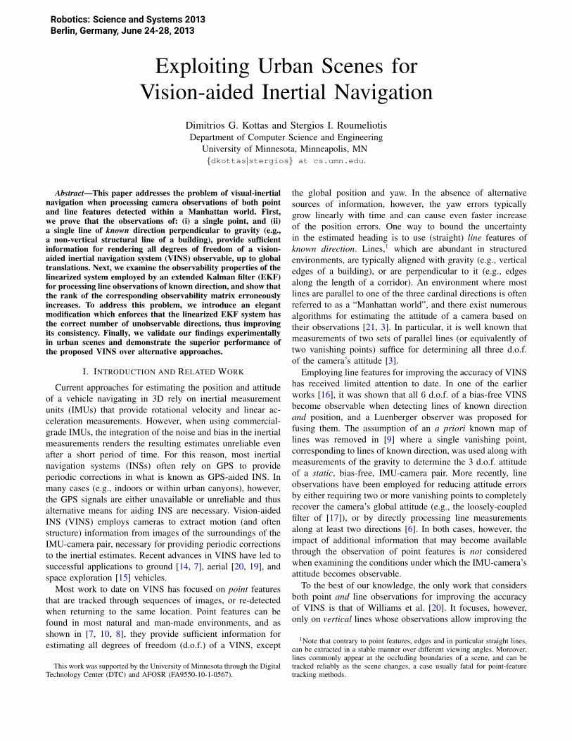
Fig. 1: The geometric constraint employed for deriving an inferredmeasurement model in (17).

B. Measurement Model

Due to space limitations, we omit the description of themeasurement model and the corresponding observability ma-trix for point features, since this has been investigated thor-oughly in existing literature (see [15, 8] and references there-in). Instead we hereafter focus on the measurement model,corresponding to observations of lines of known direction.

For simplicity, we assume that the IMU frame of referenceI coincides with the camera frame of reference3. The opticalcenter of the camera I, together with the 3D line l, definea plane π in space. Let O denote the principal point of theimage plane π′. The image sensor captures the intersectionline l′ of the plane π and π′, and parameterizes it by an angleφ and distance ρ (see Fig. 1).

A point p with homogeneous image coordinates pT =[u v 1

], lies on the line l′ if it satisfies the equality:[

cosφ sinφ −ρ]p = 0. (12)

Let Iu =[sinφ − cosφ 0

]Tbe a (free) unit vector along

the line l′ on the image plane and let P denote the pointon l′ that is closest to O. From Fig. 1, the vectors Iu andIP = IO+OP =

[ρ cosφ ρ sinφ 1

]Tdefine the plane π.

The unit vector In, perpendicular to the plane π, is:

In =IP × Iu

||IP × Iu||2=

1√1 + ρ2

[cosφ sinφ −ρ

]T. (13)

So as to couple the VINS state with the known line directionGl, we formulate the following geometric constraint:

h(x, In) = InTC(I qG)Gl = 0 (14)

which captures the fact that the line direction Gl, expressedin the IMU frame I, lies in the plane π, and henceis perpendicular to the normal In. In practice, the camerameasures4

z =[φ ρ

]T+ ξ (15)

where ξ follows a zero-mean Gaussian distributionN (02×1,Rφρ) and represents the noise induced by the

3In practice, we perform IMU-camera extrinsic calibration following theapproach of [12].

4We estimate φ and ρ, and their associated covariances by fitting a straightline to points that belong to an image edge.

camera sensor and the line extraction algorithm. The effectof ξ on h(x, In), denoted by w can be approximated throughlinearization as:

w ≈ A1×3B3×2ξ (16)

where A = ∇Inh and B =[∇φIn ∇ρIn

]. Hence, w

can be approximated by a zero-mean Gaussian distributionN (0, σ2), σ2 = ABRφρB

TAT .Using the above noise parameterization, we arrive at the

following inferred measurement model that couples the mea-surement of line l at time-step tk, with the VINS state vector,xk:

zl,tk = h(xk,Ikn) + wk = IknTC(Ik qG)Gl + wk. (17)

The measurement Jacobian of line l, at time-step tk, takes theform:

Hlk =

[IknT bC(Ik qG)Gl×c 01×15

]. (18)

III. OBSERVABILITY ANALYSIS

In this section, we study the observability properties of aVINS observing a single point feature and a line of knowndirection, over k time steps. The observability matrix M, ofthe linearized VINS, can be partitioned in two sub-matrices(see (19)), corresponding to measurements of a point featureand a single line of known direction, respectively:

M =

Mf

—Ml

=

Hf1

Hf2Φ2,1

...HfkΦk,1

—Hl

1

Hl2Φ2,1

...HlkΦk,1

. (19)

As it has been recently shown [5], the right nullspace of Mf ,is spanned by:

Nf =

03 C (I1 qG) Gg03 03×103 −bGvI1 ×cGg03 03×1I3 −bGpI1 ×cGgI3 −bGf ×cGg

=[Nt,1 | Nr,1

]. (20)

Notice that the three directions Nt,1 correspond to globaltranslations of the platform and the observed feature, whileNr,1, describes rotations around the gravitational accelerationvector, Gg. As we show in Appendix A, the right nullspace ofMl, is given by:

Nl =

C (I1 qG) Gl 03×1203×1 03×12012×1 I12×12

=[Nl,(:,1) Nl,(:,2:13)

].

(21)

Hence, the right nullspace M is:

null(M) = range(Nf ) ∩ range(Nl). (22)

The subspace range(Nf )∩range(Nl) can be parameterized as:

NfNα = NlNβ (23)

for full column rank matrices Nα, Nβ . From (23), we get:[Nf | −Nl

] [Nα

Nβ

]︸ ︷︷ ︸

∆

= 0. (24)

Hence ∆ is the right nullspace of[Nf | −Nl

], which is:

∆ =

I301×301×303

03

I3I3

, if Gl 6‖ Gg

I3 03×101×3 101×3 γ03 −bGvI1 ×cGg03 03×1I3 −bGpI1 ×cGgI3 −bGf×cGg

, otherwise.

where γ is a scalar such that Gg = γGl. After recovering Nα,we get the span of range(Nf ) ∩ range(Nl) as:

null(M) = NfNα =

[Nt,1

]if Gl 6‖ Gg[

Nt,1 | Nr,1

]otherwise.

In summary, we have shown that observations of a single pointfeature and a single 3D line of known direction, different fromgravity, provide enough information, for rendering all degreesof freedom of a VINS observable, up to the global translationsof the observed feature and the IMU-camera platform.

IV. CONSISTENT EKF UPDATES FORLINES OF KNOWN DIRECTION

As defined in [1], a state estimator is consistent if theestimation errors are zero-mean and have covariance smallerthan or equal to the one calculated by the filter. Unfortunately,processing observations of lines of known direction using anEKF can lead to injection of spurious information and henceinconsistencies.

As we show in Appendix A, for the true linearized sys-tem, the direction corresponding to rotations around l isunobservable and the observability matrix Ml is of rank 5.However, when the system and measurement Jacobians areevaluated at the current state estimates, the correspondingobservability matrix Ml becomes of rank 6. This causes theEKF to erroneously perceive the direction corresponding torotations around the known line l as observable and decreaseits uncertainty, causing estimator inconsistency. We hereafter

examine this problem in more detail and propose a simple, yetpowerful, method for addressing it.

Consider a system observing a single line of known direc-tion l over k time-steps, t1, . . . , tk. For the linearized system,employed by the EKF the first row of the observability matrixMl, takes the form:5

Ml1 =

[I1nT bC (I1|0 qG) Gl×c 01×3 01×12

](25)

while its k − th row has the form:

Mlk =

[IknT bC (Ik|k−1 qG) Gl×cΓk Ek 01×12

]. (26)

where:

Γk = Φ(1,1)k|k−1,k−1|k−1 . . .Φ

(1,1)2|1,1|1 (27)

= C(Ik|k−1 qIk−1|k−1

). . .C

(I2|1 qI1|1

)and Ek is a time-varying full-rank matrix that does not affectthe present analysis.

From the structure of the observability matrix Ml, thedirections Nl,(:,2:13) (see (21)) are independent of the currentstate estimate and satisfy Ml

kNl,(:,2:13) = 0, for any k.

However, the same is not true for the direction Nl,(:,1) whichcorresponds to rotations around the line l.

Specifically, at time-step t1, the direction Nl,(:,1) is givenby:

Nl,(:,1)1|0 =

C (I1|0 qG) Gl03×1012×1

. (28)

For MlkN

l,(:,1)1|0 = 0 to hold, we would need:

IknT bC (Ik|k−1 qG) Gl×cΓkC (I1|0 qG) Gl = 0, ∀ k (29)

which in general does not hold, for the Γk in (27) and leadsto injection of spurious information. To address this problem,we seek a modified Γ?k such that:

Γ?kC (I1|0 qG) Gl = C (Ik|k−1 qG) Gl. (30)

One possible solution, for (30), is to evaluate Φ(1,1), usingthe propagated orientation estimates, i.e.,

Φ?(1,1)k|k−1,k−1|k−1 = C

(Ik|k−1 qIk−1|k−2

). (31)

In that case, the k− th row of the observability matrix wouldinclude a matrix Γ?k such that:

Γ?k = C(Ik|k−1 qIk−1|k−2

). . .C

(I2|1 qI1|0

)(32)

which satisfies (30).

V. VINS IN AN URBAN SCENE ALIGNED WITH GRAVITY

We make the assumption that we navigate in an environ-ment whose lines are predominantly mutually orthogonal andaligned with the gravitational field (i.e., parallel or perpendic-ular to the gravity vector). After initializing the roll and pitchangles w.r.t. a global frame G, whose z-axis is parallel togravity, finding the initial yaw is achieved through the processdescribed hereafter.

5Ik|k−1 denotes the estimate for frame I at time-step k, utilizing allavailable inertial measurements and line observations only up to time-stepk − 1.

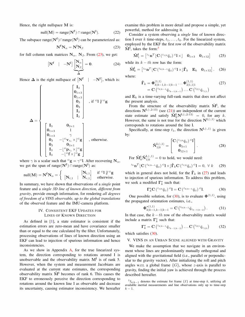
A. Yaw Initialization

Firstly, we employ a RANSAC-based vanishing point esti-mator that uses triplets of lines for generating hypotheses ofall three orthogonal vanishing points at once [13]. We prunethese hypotheses, by keeping the one that corresponds to arotational matrix with roll and pitch angles closest to thoseestimated by the filter. Following this method, we define aframe B (corresponding to the building) whose cardinalaxes are aligned with the structural lines of the scene. Next,we estimate the yaw angle, θ, between frames G and B.As an example, consider N observations, ni, i = 1 . . . N ,of lines parallel to the direction e1 =

[1 0 0

]Tof the

building. From these measurements, we arrive at the followingleast squares problem:

minθ

J(θ) (33)

J(θ) =

N∑i=1

nTi C(I qG)

cos(θ) sin(θ) 0− sin(θ) cos(θ) 0

0 0 1

e1

2

After defining,

u =

[cos(θ)sin(θ)

], and Π =

1 00 −10 0

(34)

we can re-arrange J(θ) as,

J(u) =

N∑i=1

(nTi C(I qG)Πu

)2= uT ΠTC(I qG)T

N∑i=1

(nin

Ti

)C(I qG)Π︸ ︷︷ ︸

S

u (35)

When uT u = 1, (35) corresponds to the Rayleigh quotient ofthe matrix S and is minimized for a u∗ equal to the eigenvectorcorresponding to the minimum eigenvalue of S. Hence, werecover θ, as: [

cos(θ)sin(θ)

]= ±u∗ (36)

Note, that this procedure takes place once, at the initializa-tion of the filter, so as to disambiguate the cardinal directionsof the building. Hereafter, we assume that the cardinal axesof the frame G are parallel with the cardinal axes of thebuilding.

B. Line Classification

After we perform gradient edge detection using the CannyEdge detector [2] and extract straight lines using OpenCV’sprobabilistic Hough transform [11], we need to classifywhether a line is parallel to one of the three cardinal directions,ej , j = 1 . . . 3:

e1 =

100

, e2 =

010

, e3 =

001

. (37)

Fig. 2: Lines corresponding to the building’s x cardinal axis,classified using a RANSAC-based vanishing point estimator, forperforming heading (yaw) initialization.

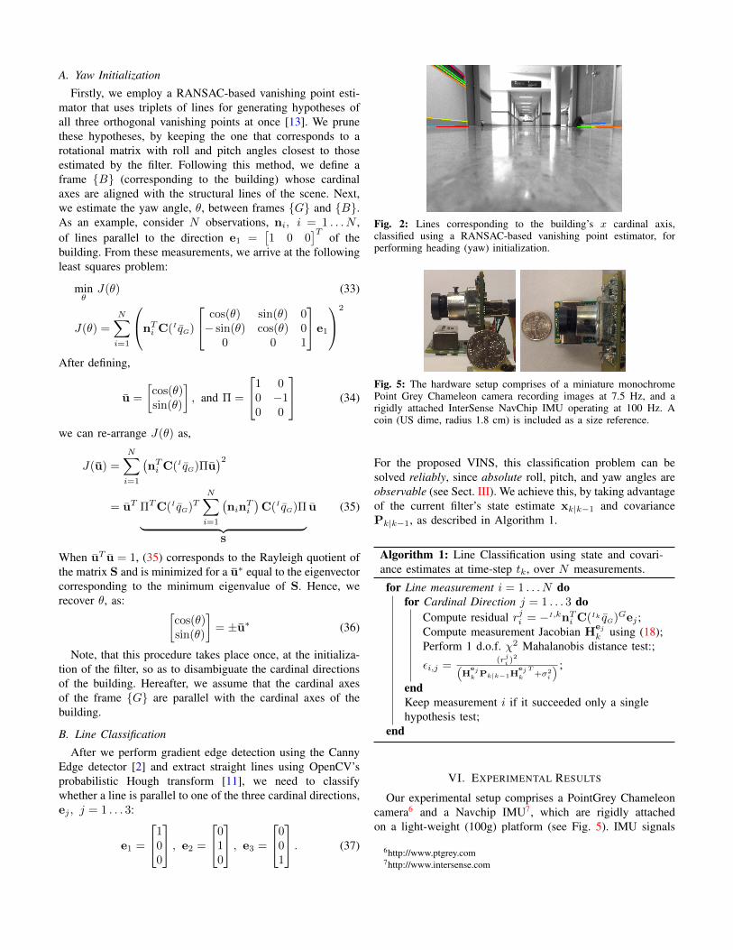
Fig. 5: The hardware setup comprises of a miniature monochromePoint Grey Chameleon camera recording images at 7.5 Hz, and arigidly attached InterSense NavChip IMU operating at 100 Hz. Acoin (US dime, radius 1.8 cm) is included as a size reference.

For the proposed VINS, this classification problem can besolved reliably, since absolute roll, pitch, and yaw angles areobservable (see Sect. III). We achieve this, by taking advantageof the current filter’s state estimate xk|k−1 and covariancePk|k−1, as described in Algorithm 1.

Algorithm 1: Line Classification using state and covari-ance estimates at time-step tk, over N measurements.

for Line measurement i = 1 . . . N dofor Cardinal Direction j = 1 . . . 3 do

Compute residual rji = −I,knTi C(Ik qG)Gej ;Compute measurement Jacobian H

ejk using (18);

Perform 1 d.o.f. χ2 Mahalanobis distance test:;

εi,j =(rji )

2(H

ejk Pk|k−1H

ejk

T+σ2

i

) ;

endKeep measurement i if it succeeded only a singlehypothesis test;

end

VI. EXPERIMENTAL RESULTS

Our experimental setup comprises a PointGrey Chameleoncamera6 and a Navchip IMU7, which are rigidly attachedon a light-weight (100g) platform (see Fig. 5). IMU signals

6http://www.ptgrey.com7http://www.intersense.com

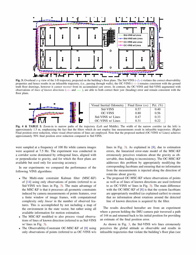
Fig. 3: Overhead x-y view of the 3-D trajectory, projected on the building’s floor plans. The Std-VINS (–4–) violates the correct observabilityproperties and hence results in an infeasible trajectory, (i.e., passing through walls), the OC-VINS (–×–) remains consistent with the groundtruth floor drawings, however it cannot recover from its accumulated yaw errors. In contrast, the OC-VINS and Std-VINS augmented withobservations of lines of known directions (–– and —– ), are able to both correct their yaw (heading) error and remain consistent with thefloor plans.

Visual Inertial Odometry Final Error (m) Pct. (%)Std-VINS 0.57 0.40OC-VINS 0.80 0.56

Std-VINS w/ Lines 0.47 0.33OC-VINS w/ Lines 0.31 0.22

Fig. 4 & TABLE I: Zoom-in to narrow paths of the trajectory (Left and Middle). The width of the narrow corridor (at the left) isapproximately 1.5 m, emphasizing the fact that the filters which do not employ line measurements result in infeasible trajectories. (Right)Final position error reduction, when visual observations of lines are employed. Note that the proposed method (OC-VINS w/ Lines) achievesapproximately 50% final position error reduction compared to Std-VINS.

were sampled at a frequency of 100 Hz while camera imageswere acquired at 7.5 Hz. The experiment was conducted ina corridor scene dominated by orthogonal lines, aligned withor perpendicular to gravity, and for which the floor plans areavailable but used only for assessing accuracy.

In our experiments we compared the performance of thefollowing VINS algorithms:

• The Multi-state constraint Kalman filter (MSC-KF)of [14] using only observations of points (referred to asStd-VINS w/o lines in Fig. 3). The main advantage ofthe MSC-KF is that it processes all geometric constraintsinduced by camera measurements of points features, overa finite window of image frames, with computationalcomplexity only linear in the number of observed fea-tures. This is accomplished by not including a map ofthe environment in the state vector, but rather using allavailable information for motion estimation.

• The MSC-KF modified to also process visual observa-tions of lines of known direction (referred to as Std-VINSw/ lines in Fig. 3).

• The Observability-Constraint OC-MSC-KF of [8] usingonly observations of points (referred to as OC-VINS w/o

lines in Fig. 3). As explained in [8], due to estimationerrors, the linearized error-state model of the MSC-KFerroneously perceives rotations about the gravity as ob-servable, thus leading to inconsistency. The OC-MSC-KFaddresses this problem by appropriately modifying thecorresponding Jacobians and ensuring that no informationfrom the measurements is injected along the direction ofrotations about gravity.

• The proposed OC-MSC-KF where observations of pointsas well as of lines of known directions are used (referredto as OC-VINS w/ lines in Fig. 3). The main differencewith the OC-MSC-KF of [8] is that the system Jacobiansare appropriately modified (as explained earlier) to ensurethat no information about rotations around the detectedline of known direction is acquired by the filter.

The results described hereafter are from an experimentwhere a person holding the IMU-camera pair traversed a pathof 144 m and returned back to his initial position for providingan estimate of the final position error.

As shown in Fig. 3, the Std-VINS w/o lines erroneouslyperceives the global attitude as observable and results ininfeasible trajectories that violate the building’s floor plan (see

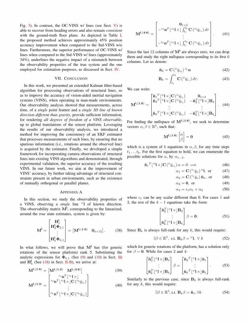
Fig. 3). In contrast, the OC-VINS w/ lines (see Sect. V) isable to recover from heading errors and also remain consistentwith the ground-truth floor plans. As depicted in Table I,the proposed method achieves approximately 45% positionaccuracy improvement when compared to the Std-VINS w/olines. Furthermore, the superior performance of OC-VINS w/lines when compared to the Std-VINS w/ lines (approximately34%), underlines the negative impact of a mismatch betweenthe observability properties of the true system and the oneemployed for estimation purposes, as discussed in Sect. IV.

VII. CONCLUSION

In this work, we presented an extended Kalman filter-basedalgorithm for processing observations of structural lines, soas to improve the accuracy of vision-aided inertial navigationsystems (VINS), when operating in man-made environments.Our observability analysis showed that measurements, acrosstime, of a single point feature and a single 3D line of knowndirection different than gravity, provide sufficient information,for rendering all degrees of freedom of a VINS observable,up to global translations of the sensor platform. Leveragingthe results of our observability analysis, we introduced amethod for improving the consistency of an EKF estimatorthat processes measurements of such lines, by ensuring that nospurious information (i.e., rotations around the observed line)is acquired by the estimator. Finally, we developed a simpleframework for incorporating camera observations of structurallines into existing VINS algorithms and demonstrated, throughexperimental validation, the superior accuracy of the resultingVINS. In our future work, we aim at the improvement ofVINS’ accuracy, by further taking advantage of structural con-straints present in urban environments, such as the existenceof mutually orthogonal or parallel planes.

APPENDIX A

In this section, we study the observability properties ofa VINS, observing a single line Gl of known direction.The observability matrix Ml, corresponding to the linearized,around the true state estimates, system is given by:

Ml =

Hl

1

Hl2Φ2,1

...HlkΦk,1

=[Ml,(1:6) 0k×12

]. (38)

In what follows, we will prove that Ml has (for genericrotations of the sensor platform) rank 5. Substituting theanalytic expressions for Φk,1 (See (9) and (10) in Sect. II)and Hl

k (See (18) in Sect. II-B), we arrive at:

Ml,(1:6) =[Ml,(1:3) Ml,(4:6)

](39)

Ml,(1:3) =

I1nT bI1 l×c

I2nT bI2 l×cC (I2 qI1)...

IknT bIk l×cC (Ik qI1)

(40)

Ml,(4:6) =

01×3

−I2nT bI2 l×c∫ t2t1

C (I2 qIτ ) dτ...

−IknT bIk l×c∫ tkt1

C (Ik qIτ ) dτ

. (41)

Since the last 12 columns of Ml are always zero, we can dropthem and study the right nullspace corresponding to its first 6columns. Let us denote:

nk = C (GqIk) Ikn (42)

Bk =

∫ tk

t1

C (GqIτ ) dτ. (43)

We can write:

Ml,(1:6) =

n1

T bGl×cC (GqI1) 01×3n2

T bGl×cC (GqI1) −nT2 bGl×cB2

......

nkT bGl×cC (GqI1) −nTk bGl×cBk

. (44)

For finding the nullspace of Ml,(1:6), we seek to determinevectors α, β ∈ R3, such that:

Ml,(1:6)

[αβ

]= 0 (45)

which is a system of k equations in α, β, for any time stepst1 . . . tk. For the first equation to hold, we can enumerate thepossible solutions for α, by α1...4.

n1T bGl×cC (GqI1)α = 0 =⇒ (46)

α1 = C (I1 qG) Gl, or (47)α2 = C (I1 qG) n1, or (48)α3 = 0, or (49)α4 = ε1α1 + α2 (50)

where ε1 can be any scalar different than 0. For cases 1 and3, the rest of the k − 1 equations take the form:nT2 bGl×cB2

...nTk bGl×cBk

β = 0. (51)

Since Bk is always full-rank for any k, this would require:

∃β ∈ R3, s.t. Bkβ = Gl, ∀ k (52)

which for generic rotations of the platform, has a solution onlyfor β = 0. While for cases 2 and 4:nT2 bGl×cB2

...nTk bGl×cBk

β =

n2T bGl×cn1

...nk

T bGl×cn1

. (53)

Similarly to the previous case, since Bk is always full-rankfor any k, this would require:

∃β ∈ R3, s.t. Bkβ = n1,∀k (54)

which for generic rotations of the platform, has no solution.This concludes our proof that the right nullspace of Ml, is:

Nl =

C (I1 qG) Gl 03×1203×1 03×12012×1 I12×12

. (55)

REFERENCES

[1] Y. Bar-Shalom, X. Rong Li, and Kirubarajan T. Estima-tion with Applications to Tracking and Navigation. JohnWiley & Sons, New York, NY, 2001.

[2] J. Canny. A computational approach to edge detection.IEEE Trans. on Pattern Analysis and Machine Intelli-gence, 8(6):679–698, November 1986.

[3] H. H. Chen. Pose determination from line-to-planecorrespondences: existence condition and closed-formsolutions. IEEE Trans. on Pattern Analysis and MachineIntelligence, 13(6):530–541, June 1991.

[4] J.A. Hesch, D.G. Kottas, S.L. Bowman, and S.I. Roume-liotis. Observability-constrained Vision-aided InertialNavigation. Technical Report 2012-001, Universityof Minnesota, Dept. of Comp. Sci. & Eng., MARSLab, February 2012. URL http://www-users.cs.umn.edu/∼dkottas/pdfs/vins tr winter 2012.pdf.

[5] J.A. Hesch, D.G. Kottas, S.L. Bowman, and S.I. Roume-liotis. Towards consistent vision-aided inertial naviga-tion. In Int. Workshop on the Algorithmic Foundationsof Robotics, Cambridge, MA, June 13–15, 2012.

[6] M. Hwangbo and T. Kanade. Visual-Inertial UAV attitudeestimation using urban scene regularities. In Proc. ofthe IEEE Int. Conf. on Robotics and Automation, pages2451–2458, Shanghai, China, May 9–13, 2011.

[7] E.S. Jones and S. Soatto. Visual-inertial navigation,mapping and localization: A scalable real-time causalapproach. Int. Journal of Robotics Research, 30(4):407–430, April 2011.

[8] D.G. Kottas, J.A. Hesch, S.L. Bowman, and S.I. Roume-liotis. On the consistency of vision-aided inertial nav-igation. In Int. Symposium on Experimental Robotics,Quebec City, Canada, June 17–21, 2012.

[9] J. Lobo and J. Dias. Vision and inertial sensor cooper-ation using gravity as a vertical reference. IEEE Trans.on Pattern Analysis and Machine Intelligence, 25(12):1597–1608, Dec 2003.

[10] A. Martinelli. Vision and IMU data fusion: Closed-formsolutions for attitude, speed, absolute scale, and biasdetermination. IEEE Trans. on Robotics, 28(1):44–60,February 2012.

[11] J. Matas, C. Galambos, and J. Kittler. Robust detection oflines using the progressive probabilistic hough transform.Computer Vision and Image Understanding, 78(1):119–137, April 2000.

[12] F.M. Mirzaei and S.I. Roumeliotis. A Kalman filter-based algorithm for IMU-camera calibration: Observabil-ity analysis and performance evaluation. IEEE Trans. onRobotics, 24(5):1143–1156, October 2008.

[13] F.M. Mirzaei and S.I. Roumeliotis. Optimal estimation ofvanishing points in a manhattan world. In Proc. of the Int.Conf. on Computer Vision, pages 2454–2461, Barcelona,Spain, November 6-12 2011. IEEE.

[14] A.I. Mourikis and S.I Roumeliotis. A multi-state con-straint Kalman filter for vision-aided inertial navigation.In Proc. of the IEEE Int. Conf. on Robotics and Automa-tion, pages 3565–3572, Rome, Italy, April 10–14, 2007.

[15] A.I Mourikis, N. Trawny, S.I Roumeliotis, A.E. Johnson,A. Ansar, and L. Matthies. Vision-aided inertial naviga-tion for spacecraft entry, descent, and landing. IEEETrans. on Robotics, 25(2):264–280, April 2009.

[16] H. Rehbinder and B.K. Ghosh. Pose estimation us-ing line-based dynamic vision and inertial sensors.IEEE Transactions on Automatic Control, 48(2):186–199, February 2003.

[17] L. Ruotsalainen, J. Bancroft, and G. Lachapelle. Miti-gation of attitude and gyro errors through vision aiding.In Proc. of the IEEE Int. Conf. on Indoor Positioningand Indoor Navigation, pages 1–9, Sydney, Australia,November 13–15, 2012.

[18] N. Trawny and S. I. Roumeliotis. Indirect Kalman filterfor 3D attitude estimation. Technical Report 2005-002,University of Minnesota, Dept. of Comp. Sci. & Eng.,MARS Lab, March 2005. URL http://www-users.cs.umn.edu/∼trawny/Publications/Quaternions 3D.pdf.

[19] S. Weiss, M.W. Achtelik, S. Lynen, M. Chli, and R. Sieg-wart. Real-time onboard visual-inertial state estimationand self-calibration of MAVs in unknown environment.In Proc. of the IEEE Int. Conf. on Robotics and Automa-tion, St. Paul, MN, May 14–18, 2012.

[20] B. Williams, N. Hudson, N. Tweddle, R. Brockers, andL. Matthies. Feature and pose constrained visual aidedinertial navigation for computationally constrained aerialvehicles. In Proc. of the IEEE Int. Conf. on Roboticsand Automation, pages 431–438, Shanghai, China, May9–13, 2011.

[21] T.S. Huang Y. Liu and O.D. Faugeras. Determination ofcamera location from 2D to 3D line and point correspon-dences. In Proc. of the IEEE Conf. on Computer Visionand Pattern Recognition, pages 82–88, Ann Arbor, MI,June 5–9, 1988.