Exploiting linguistic knowledge to infer properties of ...pcook/Cook2010.pdfExploiting linguistic...
154
Exploiting linguistic knowledge to infer properties of neologisms by C. Paul Cook A thesis submitted in conformity with the requirements for the degree of Doctor of Philosophy Graduate Department of Computer Science University of Toronto c Copyright by C. Paul Cook 2010
-
Upload
hoangkhuong -
Category
Documents
-
view
225 -
download
0
Transcript of Exploiting linguistic knowledge to infer properties of ...pcook/Cook2010.pdfExploiting linguistic...
Exploiting linguistic knowledge to infer properties of
neologisms
by
C. Paul Cook
A thesis submitted in conformity with the requirementsfor the degree of Doctor of Philosophy
Graduate Department of Computer Science
University of Toronto
c© Copyright by C. Paul Cook 2010
Abstract
Exploiting linguistic knowledge to infer properties of neologisms
C. Paul Cook
Doctor of Philosophy
Graduate Department of Computer Science
University of Toronto
2010
Neologisms, or newly-coined words, pose problems for natural language processing
(NLP) systems. Due to the recency of their coinage, neologisms are typically not listed
in computational lexicons—dictionary-like resources that many NLP applications depend
on. Therefore when a neologism is encountered in a text being processed, the performance
of an NLP system will likely suffer due to the missing word-level information. Identifying
and documenting the usage of neologisms is also a challenge in lexicography, the making
of dictionaries. The traditional approach to these tasks has been to manually read a lot of
text. However, due to the vast quantities of text being produced nowadays, particularly
in electronic media such as blogs, it is no longer possible to manually analyze it all
in search of neologisms. Methods for automatically identifying and inferring syntactic
and semantic properties of neologisms would therefore address problems encountered in
both natural language processing and lexicography. Because neologisms are typically
infrequent due to their recent addition to the language, approaches to automatically
learning word-level information relying on statistical distributional information are in
many cases inappropriate. Moreover, neologisms occur in many domains and genres, and
therefore approaches relying on domain-specific resources are also inappropriate. The
hypothesis of this thesis is that knowledge about etymology—including word formation
processes and types of semantic change—can be exploited for the acquisition of aspects
of the syntax and semantics of neologisms. Evidence supporting this hypothesis is found
ii
in three case studies: lexical blends (e.g., webisode a blend of web and episode), text
messaging forms (e.g., any1 for anyone), and ameliorations and pejorations (e.g., the
use of sick to mean ‘excellent’, an amelioration). Moreover, this thesis presents the first
computational work on lexical blends and ameliorations and pejorations, and the first
unsupervised approach to text message normalization.
iii

Dedication
To my beautiful wife Hannah for loving and supporting me through the ups and downs
of life.
iv

Acknowledgements
I’d like to begin by thanking my supervisor, Suzanne Stevenson, for her support through-
out my graduate studies. Suzanne, thanks for believing in me when I told you that I
wanted to work on, of all things, lexical blends. Thank you for having the confidence
in me to let me work on understudied phenomena and do research that is truly novel.
Without your support this thesis wouldn’t even have been started.
I’d also like to thank the other members of my thesis committee, Graeme Hirst and
Gerald Penn. Their feedback on my research and their careful reading of my thesis
greatly improved the quality of my work.
I’m also grateful to my collaborator, Afsaneh Fazly. Although the research that we
did together did not form a part of this thesis, working with Afsaneh, and learning from
her experience and insight, was an important part of my development as a researcher.
I’d further like to thank the other members, past and present, of the computational
linguistics group at the University of Toronto. Their feedback and support has been a
tremendous help throughout my Ph.D.
Finally I’d like to thank the Natural Sciences and Engineering Research Council of
Canada, the Ontario Graduate Scholarship Program, the University of Toronto, and the
Dictionary Society of North America for financially supporting this research.
v
Contents
1 Neologisms 1
1.1 Problems posed by neologisms . . . . . . . . . . . . . . . . . . . . . . . . 4
1.1.1 Challenges for natural language processing . . . . . . . . . . . . . 4
1.1.2 Problems in lexicography . . . . . . . . . . . . . . . . . . . . . . . 6
1.2 New word typology . . . . . . . . . . . . . . . . . . . . . . . . . . . . . . 7
1.3 Overview of thesis . . . . . . . . . . . . . . . . . . . . . . . . . . . . . . . 9
2 Related work 12
2.1 Computational work on specific word formations . . . . . . . . . . . . . . 13
2.1.1 Composites . . . . . . . . . . . . . . . . . . . . . . . . . . . . . . 13
2.1.1.1 POS tagging . . . . . . . . . . . . . . . . . . . . . . . . 13
2.1.1.2 Compounds . . . . . . . . . . . . . . . . . . . . . . . . . 15
2.1.2 Shifts . . . . . . . . . . . . . . . . . . . . . . . . . . . . . . . . . 16
2.1.3 Shortenings . . . . . . . . . . . . . . . . . . . . . . . . . . . . . . 18
2.1.3.1 Acronyms and initialisms . . . . . . . . . . . . . . . . . 18
2.1.3.2 Clippings . . . . . . . . . . . . . . . . . . . . . . . . . . 21
2.1.4 Loanwords . . . . . . . . . . . . . . . . . . . . . . . . . . . . . . . 22
2.1.5 Blends . . . . . . . . . . . . . . . . . . . . . . . . . . . . . . . . . 24
2.2 Computational work exploiting context . . . . . . . . . . . . . . . . . . . 24
2.3 Lexicographical work on identifying new words . . . . . . . . . . . . . . . 28
vi
2.3.1 Corpora in lexicography . . . . . . . . . . . . . . . . . . . . . . . 28
2.3.1.1 Drudgery . . . . . . . . . . . . . . . . . . . . . . . . . . 28
2.3.1.2 Corpora . . . . . . . . . . . . . . . . . . . . . . . . . . . 29
2.3.1.3 Statistics . . . . . . . . . . . . . . . . . . . . . . . . . . 30
2.3.2 Successful new words . . . . . . . . . . . . . . . . . . . . . . . . . 32
2.3.3 Finding new words . . . . . . . . . . . . . . . . . . . . . . . . . . 37
3 Lexical blends 41
3.1 A statistical model of lexical blends . . . . . . . . . . . . . . . . . . . . . 43
3.1.1 Candidate sets . . . . . . . . . . . . . . . . . . . . . . . . . . . . 43
3.1.2 Statistical features . . . . . . . . . . . . . . . . . . . . . . . . . . 44
3.1.2.1 Frequency . . . . . . . . . . . . . . . . . . . . . . . . . . 45
3.1.2.2 Length, contribution, and phonology . . . . . . . . . . . 47
3.1.2.3 Semantics . . . . . . . . . . . . . . . . . . . . . . . . . . 49
3.1.2.4 Syllable structure . . . . . . . . . . . . . . . . . . . . . . 50
3.2 Creating a dataset of recent blends . . . . . . . . . . . . . . . . . . . . . 50
3.3 Materials and methods . . . . . . . . . . . . . . . . . . . . . . . . . . . . 53
3.3.1 Experimental expressions . . . . . . . . . . . . . . . . . . . . . . . 53
3.3.2 Experimental resources . . . . . . . . . . . . . . . . . . . . . . . . 54
3.3.3 Experimental methods . . . . . . . . . . . . . . . . . . . . . . . . 55
3.3.4 Evaluation metrics . . . . . . . . . . . . . . . . . . . . . . . . . . 57
3.4 Experimental results . . . . . . . . . . . . . . . . . . . . . . . . . . . . . 57
3.4.1 Candidate sets . . . . . . . . . . . . . . . . . . . . . . . . . . . . 57
3.4.1.1 CELEX . . . . . . . . . . . . . . . . . . . . . . . . . . . 58
3.4.1.2 Web 1T 5-gram Corpus . . . . . . . . . . . . . . . . . . 59
3.4.2 Source word identification . . . . . . . . . . . . . . . . . . . . . . 59
3.4.2.1 Feature ranking . . . . . . . . . . . . . . . . . . . . . . . 60
3.4.2.2 Error analysis . . . . . . . . . . . . . . . . . . . . . . . . 62
vii
3.4.2.3 Modified perceptron . . . . . . . . . . . . . . . . . . . . 64
3.4.2.4 Discussion . . . . . . . . . . . . . . . . . . . . . . . . . . 65
3.5 Blend identification . . . . . . . . . . . . . . . . . . . . . . . . . . . . . . 66
3.6 Related Work . . . . . . . . . . . . . . . . . . . . . . . . . . . . . . . . . 68
3.7 Summary of contributions . . . . . . . . . . . . . . . . . . . . . . . . . . 70
4 Text message forms 71
4.1 Analysis of texting forms . . . . . . . . . . . . . . . . . . . . . . . . . . . 74
4.2 An unsupervised noisy channel model for text message normalization . . 77
4.2.1 Word models . . . . . . . . . . . . . . . . . . . . . . . . . . . . . 78
4.2.1.1 Stylistic variations . . . . . . . . . . . . . . . . . . . . . 78
4.2.1.2 Subsequence abbreviations . . . . . . . . . . . . . . . . . 80
4.2.1.3 Suffix clippings . . . . . . . . . . . . . . . . . . . . . . . 81
4.2.2 Word formation prior . . . . . . . . . . . . . . . . . . . . . . . . . 81
4.2.3 Language model . . . . . . . . . . . . . . . . . . . . . . . . . . . . 82
4.3 Materials and methods . . . . . . . . . . . . . . . . . . . . . . . . . . . . 82
4.3.1 Datasets . . . . . . . . . . . . . . . . . . . . . . . . . . . . . . . . 82
4.3.2 Lexicon . . . . . . . . . . . . . . . . . . . . . . . . . . . . . . . . 83
4.3.3 Model parameter estimation . . . . . . . . . . . . . . . . . . . . . 83
4.3.4 Evaluation metrics . . . . . . . . . . . . . . . . . . . . . . . . . . 85
4.4 Results and discussion . . . . . . . . . . . . . . . . . . . . . . . . . . . . 85
4.4.1 Results by formation type . . . . . . . . . . . . . . . . . . . . . . 86
4.4.2 Results by Model . . . . . . . . . . . . . . . . . . . . . . . . . . . 89
4.4.3 All unseen data . . . . . . . . . . . . . . . . . . . . . . . . . . . . 90
4.5 Related Work . . . . . . . . . . . . . . . . . . . . . . . . . . . . . . . . . 90
4.6 Summary of contributions . . . . . . . . . . . . . . . . . . . . . . . . . . 91
viii
5 Ameliorations and pejorations 92
5.1 Determining semantic orientation . . . . . . . . . . . . . . . . . . . . . . 94
5.2 Corpora . . . . . . . . . . . . . . . . . . . . . . . . . . . . . . . . . . . . 97
5.3 Results . . . . . . . . . . . . . . . . . . . . . . . . . . . . . . . . . . . . . 100
5.3.1 Identifying historical ameliorations and pejorations . . . . . . . . 100
5.3.2 Artificial ameliorations and pejorations . . . . . . . . . . . . . . . 102
5.3.3 Hunting for ameliorations and pejorations . . . . . . . . . . . . . 104
5.4 Amelioration or pejoration of the seeds . . . . . . . . . . . . . . . . . . . 109
5.5 More on determining semantic orientation . . . . . . . . . . . . . . . . . 111
5.5.1 Combining information from the seed words . . . . . . . . . . . . 111
5.5.2 Number of seed words . . . . . . . . . . . . . . . . . . . . . . . . 112
5.5.3 Latent Semantic Analysis . . . . . . . . . . . . . . . . . . . . . . 115
5.6 Summary of contributions . . . . . . . . . . . . . . . . . . . . . . . . . . 117
6 Conclusions 118
6.1 Summary of contributions . . . . . . . . . . . . . . . . . . . . . . . . . . 118
6.2 Future directions . . . . . . . . . . . . . . . . . . . . . . . . . . . . . . . 121
6.2.1 Lexical blends . . . . . . . . . . . . . . . . . . . . . . . . . . . . . 121
6.2.2 Text messaging forms . . . . . . . . . . . . . . . . . . . . . . . . . 122
6.2.3 Ameliorations and pejorations . . . . . . . . . . . . . . . . . . . . 123
6.2.4 Corpus-based studies of semantic change . . . . . . . . . . . . . . 125
Bibliography 126
ix
List of Tables
1.1 Word formation types and their proportion in the data analyzed by Algeo
(1980). . . . . . . . . . . . . . . . . . . . . . . . . . . . . . . . . . . . . . 8
2.1 Metcalf’s (2002) FUDGE factors for determining whether a word will re-
main in usage. . . . . . . . . . . . . . . . . . . . . . . . . . . . . . . . . . 34
3.1 A candidate set for architourist, a blend of architecture and tourist. . . . 44
3.2 The Wordspy definition, and first citation given, for the blend staycation. 51
3.3 Types of blends and their frequency in Wordspy data. . . . . . . . . . . . 52
3.4 % of expressions (% exps) with their source words in each lexical resource
and candidate set (CS), and after applying the syllable heuristic filter on
the CELEX CS, as well as median CS size, for both the Wordsplend
and Mac-Conf datasets. . . . . . . . . . . . . . . . . . . . . . . . . . . 58
3.5 % accuracy on blends in Wordsplend and Mac-Conf using the feature
ranking approach. The size of each dataset is given in parentheses. The
lexicon employed (CELEX or WEB 1T) is indicated. The best accuracy
obtained using this approach for each dataset and lexicon is shown in
boldface. Results that are significantly better than the informed baseline
are indicated with ∗. . . . . . . . . . . . . . . . . . . . . . . . . . . . . . 60
x
3.6 % accuracy on blends in Wordsplend and Mac-Conf using the modi-
fied perceptron algorithm. The size of each dataset is given in parentheses.
The lexicon employed (CELEX or WEB 1T) is indicated. Results that
are significantly better than the informed baseline are indicated with ∗. . 64
4.1 Frequency of texting forms in the development set by formation type. . . 75
4.2 Grapheme–phoneme alignment for without. . . . . . . . . . . . . . . . . . 79
4.3 % in-top-1, in-top-10, and in-top-20 accuracy on test data using both
estimates for P (wf ). The results reported by Choudhury et al. (2007) are
also shown. . . . . . . . . . . . . . . . . . . . . . . . . . . . . . . . . . . 85
4.4 Frequency and % in-top-1 accuracy using the formation-specific model
where applicable (Specific) and all models (All) with a uniform estimate
for P (wf ), presented by formation type. . . . . . . . . . . . . . . . . . . 87
4.5 % in-top-1 accuracy on the 303 test expressions using each model individ-
ually. . . . . . . . . . . . . . . . . . . . . . . . . . . . . . . . . . . . . . . 89
5.1 Time period and approximate size of each corpus. . . . . . . . . . . . . . 97
5.2 % accuracy for inferring the polarity of expressions in GI using each corpus.
The accuracy for classifying the items with absolute calculated polarity in
the top 25% and 50% (top panel) and 75% and 100% (bottom panel) which
co-occur at least five times with seed words in the corresponding corpus
is shown. In each case, the baseline of always choosing negative polarity
and the number of items classified (N) are also shown. . . . . . . . . . . 98
5.3 % accuracy and baseline using Lampeter and approximately one-million-
word samples from CLMETEV and the BNC. The results using CLME-
TEV and the BNC are averaged over five random one-million-word samples. 99
xi
5.4 The polarity in each corpus and change in polarity for each historical
example of amelioration and pejoration. Note that succeed does not exhibit
the expected change in polarity. . . . . . . . . . . . . . . . . . . . . . . . 101
5.5 Average polarity of positive and negative words from GI in each corpus
with frequency greater than five and which co-occur at least once with
both positive and negative seed words in the indicated corpus. . . . . . . 103
5.6 Expressions with top 10 increase in polarity from CLMETEV to the BNC
(candidate ameliorations). For each expression, the proportion of human
judgements for each category is shown: CLMETEV usage is more posi-
tive/less negative (CLMETEV), BNC usage is more positive/less negative
(BNC), neither usage is more positive or negative (Neither). Majority
judgements are shown in boldface, as are correct candidate ameliorations
according to the majority responses of the judges. . . . . . . . . . . . . . 105
5.7 Expressions with top 10 decrease in polarity from CLMETEV to the BNC
(candidate pejorations). For each expression, the proportion of human
judgements for each category is shown: CLMETEV usage is more posi-
tive/less negative (CLMETEV), the BNC usage is more positive/less nega-
tive (BNC), neither usage is more positive or negative (Neither). Majority
judgements are shown in boldface, as are correct candidate pejorations
according to the majority responses of the judges. . . . . . . . . . . . . . 106
5.8 A sample of the Amazon Mechanical Turk polarity judgement task. . . . 107
5.9 Confusion matrix representing the results of our classification task used to
define our adapted versions of precision and recall (given in equations 5.6
and 5.7). . . . . . . . . . . . . . . . . . . . . . . . . . . . . . . . . . . . . 113
xii
5.10 Results for classifying items in GI in terms of our adapted versions of
precision (P), recall (R), and F-measure (F) using the TL seeds and GI
seeds. The number of seed words for each of TL and GI is given, along
with the number of items that are classified using these seed words. . . . 113
5.11 Precision (P), recall (R), F-measure (F), and number of items classified for
the top 25% most-polar items in GI. Polarity is calculated using the items
from Brooke et al.’s (2009) polarity lexicon with polarity greater than or
equal to the indicated level as seed words; the total number of seed words
is also given. . . . . . . . . . . . . . . . . . . . . . . . . . . . . . . . . . . 115
xiii
List of Figures
3.1 ROC curves for blend identification. . . . . . . . . . . . . . . . . . . . . . 67
5.1 Average % accuracy for inferring the polarity of the items in GI for each
corpus as the percentage of noisy seed words is varied. . . . . . . . . . . 110
xiv
Chapter 1
Neologisms
Neologisms—newly-coined words or new senses of an existing word—are constantly being
introduced into a language (Algeo, 1980; Lehrer, 2003), often for the purpose of naming
a new concept. Domains that are culturally prominent or that are rapidly advancing—
current examples being electronic communication and the Internet—often contain many
neologisms, although novel words do arise throughout a language (Ayto, 1990, 2006;
Knowles and Elliott, 1997).
Fischer (1998) gives the following definition of neologism:
A neologism is a word which has lost its status of a nonce-formation but is
still one which is considered new by the majority of members of a speech
community.
A nonce-formation is a word which is created and used by a speaker who believes it to be
new (Bauer, 1983); once a speaker is aware of having used or heard a word before, it ceases
to be a nonce-formation. Other definitions of neologism take a more practical stance. For
example, Algeo (1991) considers a neologism to be a word which meets the requirements
for inclusion in general dictionaries, but has not yet been recorded in such dictionaries.
The neologisms considered in this thesis will—for the most part—satisfy both of these
1
Chapter 1. Neologisms 2
definitions: they are sufficiently established to no longer be nonce-formations, generally
considered to be new, and typically not recorded in general-purpose dictionaries.
We further distinguish between two types of neologism: new words that are unique
strings of characters, for example, webisode (a blend of web and episode), and neologisms
that correspond to new meanings for an existing word form, for example, Wikipedia used
as a verb—meaning to conduct a search on the website Wikipedia—instead of as a proper
noun.
Before going any further, we must clarify the meaning of word. It is difficult to give
a definition of word which is satisfactory for all languages and all items which seem to
be words (Cruse, 2001). Therefore, in the same spirit as Cruse, we will characterize the
notion word in terms of properties of prototypical words, accepting that our definition
is inadequate for some cases. Words are typically morphological objects, that is to say
that words are formed by combining morphemes according to the rules of morphology.
Turning to syntax, specifically X-bar theory, words typically occupy the X0 position in
a parse tree; that is, words are usually syntactic atoms (Di Sciullo and Williams, 1987).
Phonological factors may also play a role in determining what is a word. For example,
a speaker typically cannot naturally pause during pronunciation of a word (Anderson,
1992). We do not appeal to the notion of listedness in the lexicon in our characterization
of word. Since the rules of morphology are recursive, there are potentially an infinite
number of words. Therefore, if the lexicon is viewed as a simple list of words, not all words
can be stored in the lexicon. Furthermore, many non-compositional phrases, such as
idioms, must be stored in the lexicon, as their meaning cannot be derived compositionally
from the meaning of their parts. Neither do we rely on whitespaces in writing to determine
what is a word. Many words are written as two whitespace delimited strings (e.g.,
many English compounds); some languages do not use whitespace to delimit words; and
moreover, some languages do not have writing systems.
Chapter 1. Neologisms 3
It is difficult to know the frequency of new word formation. Barnhart (1978, section
2.3.4) notes that approximately 500 new words are recorded each year in various English
dictionaries. This figure can be taken as a lower bound of the yearly number of new
English words, but the true number of such words is likely much higher. Dictionaries
only record words that meet their criteria for inclusion, which may be based on frequency,
range of use, timespan of use, and judgements about a word’s cruciality, that is, the need
for it to be in the language (Sheidlower, 1995). These criteria will not necessarily capture
all new words, even those that have become established in a language. Furthermore, at
the time of Barnhart’s (1978) estimate, lexicography was largely a manual undertaking.
Lexicographers identified neologisms by reading vast quantities of material and recording
what they found.1 It is entirely possible that dictionaries fail to document some of the
new words from a given time period which satisfy their criteria for inclusion.
Barnhart (1985) observes that in a large sample of magazines spanning one month,
1,000 new words were found; from this he extrapolates that the annual rate of new
word formation may be roughly 12,000 words per year. However, it is likely that many
of these terms would not be recorded in dictionaries, due to their policies for inclusion.
This figure may also be an overestimate of the yearly number of new words; sampling any
particular month will also find words which were new in a previous month, and sampling
subsequent months may reveal fewer neologisms. On the other hand, this estimate may
be quite conservative as it only considers magazines; sampling more materials may reveal
many more new words.
Metcalf (2002) claims that at least 10,000 new words are coined each day in English;
however, he also notes that most of these words never become established forms. The rate
at which new words are coined can also be estimated from corpus data. The number of
hapax legomena (or hapaxes—words which only occur once) and total number of tokens
1Johnson (1755) describes the work of dictionary making in his oft-quoted definition of lexicographer :“A writer of dictionaries; a harmless drudge, that busies himself in tracing the original, and detailingthe signification of words.”
Chapter 1. Neologisms 4
in a corpus can be used to estimate the rate of vocabulary growth (Baayen and Renouf,
1996). As corpus size increases, the proportion of new words amongst the hapaxes
increases, and so the rate of vocabulary growth gives an estimate of the rate of new
word coinage. However, new words that are also hapaxes may be nonce-formations.
Nevertheless, despite the difficulty of estimating the frequency of new word coinage, and
the differing estimates thereof, it is clear that many new words enter the English language
each year.
1.1 Problems posed by neologisms
In the following two subsections we consider challenges related to neologisms in the fields
of natural language processing and lexicography.
1.1.1 Challenges for natural language processing
Systems for natural language processing (NLP) tasks often depend on lexicons for a vari-
ety of information, such as a word’s parts-of-speech or meaning representation. Therefore,
when an unknown word—a word that is not in a system’s lexicon—is encountered in a
text being processed, the performance of the entire system will likely suffer due to missing
lexical information.
Unknown words may be of various types. For example, a word may be unknown be-
cause it is an infrequent or domain-specific word which happens to not have been included
in a system’s lexicon. For example, syntagmatic is not listed in the CELEX database
(Baayen et al., 1995), but is included in the Macquarie Dictionary (Delbridge, 1981).
Non-word spelling errors—errors that result in a form that is typically not considered to
be a word, such as teh for the—and proper nouns, are two other types of unknown word
that have received a fair amount of attention in computational linguistics, under the
headings of non-word spelling error detection and correction, and named-entity recogni-
Chapter 1. Neologisms 5
tion, respectively. Since new words are constantly being coined, neologisms are a further
source of unknown words; however, neologisms have not been studied as extensively in
computational linguistics.
Ideally, an NLP system could identify neologisms as such, and then infer various as-
pects of their syntactic or semantic properties necessary for the computational task at
hand. For example, a parser for a combinatory categorial grammar may benefit from
knowing a neologism’s syntactic category, while semantic information such as a neolo-
gism’s hypernyms may be important for tasks such as question answering. Context of
usage is clearly a key piece of information for inferring a word’s syntactic and semantic
properties, and indeed many studies into lexical acquisition have used the context in
which words occur to learn a variety of such properties (e.g., Hindle, 1990; Lapata and
Brew, 2004; Joanis et al., 2008). However, these methods are generally not applicable
for learning about neologisms. Such techniques depend on distributional information
about a word which is obtained by observing a large number of usages of that word; in
general, the more frequent a target word, the more accurate the automatically-inferred
information will be. Since neologisms are expected to be rather infrequent due to the
recency of their coinage, such methods cannot be expected to work well on these words.
On the other hand, some studies into lexical acquisition have inferred lexical in-
formation based on just a single usage, or a small number of usages, of a word (e.g.,
Granger, 1977; Cardie, 1993; Hastings and Lytinen, 1994). These methods exploit rich
representations of the lexical and syntactic context in which a given target word occurs,
as well as domain-specific knowledge resources, to infer lexical information. However,
these methods are of limited use for inferring properties of neologisms, as the domain-
specific knowledge resources they require are only available for a very small number of
narrowly-defined domains.
Chapter 1. Neologisms 6
1.1.2 Problems in lexicography
Dictionaries covering current language must be updated to reflect new words, and new
senses of existing word forms, that have come into usage. Vast quantities of text are pro-
duced each day in a variety of media including traditional publications such as newspapers
and magazines, as well as newer types of communication such as blogs and micro-blogs
(e.g., Twitter). New-word lexicographers must search this text for neologisms; however,
given the amount of text that must be analyzed, it is simply not feasible to manually
process it all (Barnhart, 1985). Therefore, automatic (or semi-automatic) methods for
the identification of new words are required.
Identifying unique string neologisms is facilitated by their distinguishing orthographic
form. One proposed method of searching for unique string neologisms that should be
included in a dictionary is to identify words that are substantially more frequent in
a corpus of recently-produced texts than in a corpus of older texts, and that are not
listed in the dictionary under consideration; the identified words can then be manually
examined, and if found to be appropriate, included in that dictionary (O’Donovan and
O’Neil, 2008). This semi-automatic method for finding new words is limited in that it
can only find unique string neologisms and not new senses of word forms. Indeed, this
remains an important open problem in computational lexicography. The precision of
such a method is also limited as it will identify new-word candidates that have unique
orthographic forms, such as jargon terms and proper nouns, that—depending on the
dictionary’s inclusion policies—should not be included in the dictionary.
Even greater challenges are posed by neologisms that correspond to new senses of
existing word forms, that is, neologisms that are homographous with words already
recorded in a given dictionary. Such neologisms result in so-called covert lexical gaps
(Zernik, 1991), which are difficult to automatically identify as they cannot be searched
for in any straightforward way. Lexicographers have also stressed the importance of
not solely focusing on new words when updating a dictionary, but also considering how
Chapter 1. Neologisms 7
established words have changed (Simpson, 2007).
1.2 New word typology
As discussed above in Section 1.1.1, current methods for lexical acquisition are generally
not applicable for learning properties of neologisms; this is largely due to the reliance of
these methods on statistical distributional information, and the tendency for neologisms
to be low-frequency items. However, knowledge about the processes through which ne-
ologisms are formed can be exploited in systems for lexical acquisition of neologisms; to
date this knowledge source has not been widely considered in computational work.
Language users create new words through a variety of word formation processes, e.g.,
derivational morphology, compounding, and borrowing from another language (Bauer,
1983; Plag, 2003). To estimate the relative frequency of the various word formation pro-
cesses, Algeo (1980) determines the etymology of 1,000 words selected from Barnhart
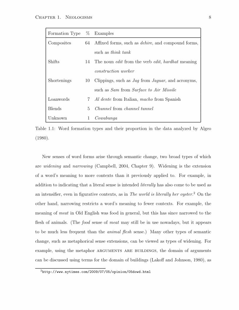
et al. (1973); a summary of his findings is presented in Table 1.1. I hypothesize that by
identifying the word formation process of a given new word, and then exploiting proper-
ties of this formation process, computational systems can infer some lexical information
from a single usage of that word without relying on expensive domain-specific knowledge
resources.
Of the items Algeo classifies as shifts, roughly half—7.7% of the total words analyzed—
do not correspond to a change in part-of-speech. These items are the neologisms that
are most difficult to identify. Although these words represent a rather small percentage
of the total number of neologisms, the rate of emergence of new senses of word forms is
not necessarily low; Barnhart et al. (1973) were manually searching for neologisms, and
they may have missed many new senses of word forms. Nevertheless, new senses of word
forms also emerge through regular processes which can be exploited in computational
systems.
Chapter 1. Neologisms 8
Formation Type % Examples
Composites 64 Affixed forms, such as dehire, and compound forms,
such as think tank
Shifts 14 The noun edit from the verb edit, hardhat meaning
construction worker
Shortenings 10 Clippings, such as Jag from Jaguar, and acronyms,
such as Sam from Surface to Air Missile
Loanwords 7 Al dente from Italian, macho from Spanish
Blends 5 Chunnel from channel tunnel
Unknown 1 Cowabunga
Table 1.1: Word formation types and their proportion in the data analyzed by Algeo
(1980).
New senses of word forms arise through semantic change, two broad types of which
are widening and narrowing (Campbell, 2004, Chapter 9). Widening is the extension
of a word’s meaning to more contexts than it previously applied to. For example, in
addition to indicating that a literal sense is intended literally has also come to be used as
an intensifier, even in figurative contexts, as in The world is literally her oyster.2 On the
other hand, narrowing restricts a word’s meaning to fewer contexts. For example, the
meaning of meat in Old English was food in general, but this has since narrowed to the
flesh of animals. (The food sense of meat may still be in use nowadays, but it appears
to be much less frequent than the animal flesh sense.) Many other types of semantic
change, such as metaphorical sense extensions, can be viewed as types of widening. For
example, using the metaphor arguments are buildings, the domain of arguments
can be discussed using terms for the domain of buildings (Lakoff and Johnson, 1980), as
2http://www.nytimes.com/2009/07/05/opinion/05dowd.html
Chapter 1. Neologisms 9
in My argument was demolished. Two further types of widening are amelioration and
pejoration; in these processes a word takes on a more positive or negative evaluation,
respectively, in the mind of the speaker. A recent amelioration is the extension of banging
from its meaning of music “having a loud, prominent, danceable beat” to “excellent” (not
specifically referring to music).3 An example pejoration is retarded acquiring the sense
of being inferior or of poor quality. I hypothesize that knowledge about specific types of
semantic change, such as amelioration and pejoration, can be exploited by computational
systems for the automatic acquisition of new senses of word forms.
1.3 Overview of thesis
The hypothesis of this thesis is that knowledge about etymology—including word for-
mation processes and types of semantic change—can be exploited for the acquisition of
aspects of the syntax and semantics of neologisms; to date, this knowledge source has not
been widely considered in computational linguistics. Moreover, in some cases, exploiting
etymological information may allow the development of lexical acquisition methods which
rely on neither statistical distributional information nor domain-specific lexical resources,
both of which are desirable to avoid in the case of neologisms.
Chapter 2 discusses related computational and lexicographical work on neologisms.
In particular, we examine computational work that has exploited knowledge of word
formation processes for lexical acquisition, as well as studies that infer aspects of the
syntax and semantics of a given lexical item from just a small number of its usages.
This chapter also examines lexicographical approaches to identifying neologisms and
determining which are likely to remain in usage, and thus deserve entry in a dictionary.
The next three chapters present novel research on three topics related to the research
discussed in Chapter 2 that, to date, have not received the attention they deserve in
3“banging, ppl. a.” OED Online, March 2007, Oxford University Press, 13 August 2009 http:
//dictionary.oed.com/cgi/entry/50017259.
Chapter 1. Neologisms 10
computational linguistics. Lexical blends—or blends, also sometimes referred to as port-
manteaux by lay people—are words such as staycation which are formed by combining
parts of existing words, in this case stay-at-home and vacation. Although accounting for
roughly 5% of new words (see Table 1.1), blends have largely been ignored in compu-
tational work. Chapter 3 presents a method for inferring the source words of a given
blend—for example, stay-at-home and vacation for staycation—based on linguistic ob-
servations about blends and their source words and cognitive factors that likely play a
role in their interpretation. On a dataset of 324 blends, the proposed method achieves an
accuracy of 40% on the task of identifying both source words of each expression, which
has an informed baseline of 27%. Chapter 3 also presents preliminary results for the task
of distinguishing blends from other types of neologisms. This research is the first com-
putational study of lexical blends, and was previously published by Cook and Stevenson
(2007) and Cook and Stevenson (2010b).
Cell phone text messaging—also known as SMS—contains many abbreviations and
non-standard forms. Before NLP tasks such as machine translation can be applied to
text messages, the text must first be normalized by converting non-standard forms to
their standard forms. This is particularly important for text messaging given the abun-
dance of non-standard forms in this medium. Although text message normalization has
been considered in several computational studies, the issue of out-of-vocabulary texting
forms—items that are encountered in text on which the system is operating, but not
found in the system’s training data—has received little attention. Chapter 4 presents an
unsupervised type-level model for normalization of non-standard texting forms. The pro-
posed method draws on observations about the typical word formation processes in text
messaging, and—like the work on lexical blends described in Chapter 3—incorporates
cognitive factors in human interpretation of text messaging forms. The performance of
the proposed unsupervised method is on par with that of the best reported results of a
supervised system on the same dataset. This work was previously published by Cook
Chapter 1. Neologisms 11
and Stevenson (2009).
The research in Chapters 3 and 4 focuses on unique string neologisms. Chapter 5,
on the other hand, presents work on identifying new word senses. Amelioration and
pejoration are common types of semantic change through which a word’s meaning takes
on a more positive or negative evaluation in the mind of the speaker. Given the re-
cent interest in natural language processing tasks such as sentiment analysis, and that
many current approaches to such tasks rely on lexicons of word-level polarity, automatic
methods for keeping polarity lexicons up-to-date are needed. Furthermore, knowledge
of word-level polarity is important for speakers—particularly non-native speakers of a
language—to use words appropriately. Tools to track changes in polarity could therefore
also be useful to lexicographers in keeping dictionaries current. Chapter 5 presents an
unsupervised statistical method for identifying ameliorations and pejorations drawing on
recent corpus-based methods for inferring semantic orientation lexicons. We show that
our proposed method is able to successfully identify historical ameliorations and pejora-
tions, as well as artificial examples of amelioration and pejoration. We also apply our
method to find words which have undergone amelioration and pejoration in recent text,
and show that this method may be used as a semi-automatic tool for finding new word
senses. This research was previously published by Cook and Stevenson (2010a) and is
the first published computational work focusing on amelioration and pejoration.
Finally, Chapter 6 gives a summary of the contributions of this thesis and identifies
potential directions for future work.
Chapter 2
Related work
As discussed in Chapter 1, neologisms pose problems for NLP applications, such as
question answering, due to the absence of lexical information for these items. Moreover,
since neologisms are expected to be rather infrequent due to the recency of their coinage,
methods for lexical acquisition that rely solely on statistical distributional information are
not well-suited for learning syntactic or semantic properties of neologisms, particularly
those which have very low frequency.
Linguistic observations regarding neologisms—namely aspects of their etymology such
as the word formation process through which whey were created—can be exploited in
systems for inferring syntactic or semantic properties of infrequent new words. In Sec-
tion 2.1 we examine computational work related to each of the word formation processes
that Algeo (1980) identifies. (See Table 1.1, page 8, for Algeo’s word formation process
classification scheme.)
The context in which a neologism is used also provides information about its syntax
and semantics. This is the intuition behind corpus-based statistical methods for lexical
acquisition which we have already discussed as not being applicable for neologisms; how-
ever, a number of methods have been proposed for inferring the syntax or semantics of
an unknown word—potentially a neologism—using domain-specific lexical resources and
12
Chapter 2. Related work 13
the context in which it occurs, based on just a single usage, or a small number of usages.
Section 2.2 examines some of this work.
Identifying and documenting new words is also a challenge for lexicography. From
the massive amounts of text produced each day, neologisms must be found; subsequently,
those neologisms that are expected to remain in the language need to be added to dictio-
naries of current usage. Section 2.3 discusses lexicographical approaches—both manual
and semi-automatic—to these tasks.
2.1 Computational work on specific word formations
In this section we examine a number of computational methods that have exploited
knowledge about the way in which new words are typically formed in order to learn
aspects of their syntax or semantics. We consider each type of word formation that
Algeo (1980) identifies, in decreasing order of frequency in the data he analyzes (see
Table 1.1, page 8).
2.1.1 Composites
In Algeo’s (1980) taxonomy of new words, the category of composites consists of words
created through derivational morphology by combining affixes with existing words, and
compounds formed by combining two words. In Section 2.1.1.1 we discuss a number of
approaches that have exploited knowledge of prefixes and suffixes for the task of part-of-
speech (POS) tagging. In Section 2.1.1.2 we look at some computational work that has
addressed compounds.
2.1.1.1 POS tagging
POS tagging of unknown words, including neologisms, can benefit greatly from exploiting
word structure. A simple method for tagging English unknown words would be to tag
Chapter 2. Related work 14
a word as a common noun if it begins with a lowercase letter, and as a proper noun
otherwise. However, there are a number of heuristics based on word endings which can
easily be incorporated to improve performance. For example, tagging of English words
can benefit from the knowledge that regular English verbs often end in -ed when used
in the past tense. Indeed, commonly used POS taggers have made use of this kind of
information.
Brill’s (1994) transformation-based tagger handles unknown words by learning weights
for lexicalized transformations specific to these words. These transformations incorpo-
rate information about suffixes and the presence of particular characters. Although the
transformations capture properties specific to English, such as to change the tag for a
word from common noun to past participle verb if the word ends in the suffix -ed, the
specific lexicalizations and corresponding weights for these transformations are learned
automatically. Ratnaparkhi (1996) assumes that unknown words in test data behave
similarly to infrequent words in training data. He also introduces some features specifi-
cally to cope with unknown words, which are based on prefixes and suffixes of a word as
well as the presence of uppercase characters.
Toutanova et al. (2003) improve on the results of Ratnaparkhi by using features
which are lexicalized on the specific words in the context of the target word (as opposed
to just their part-of-speech tags). Like Ratnaparkhi, Toutanova et al. also introduce a
small number of features specifically aimed at improving tagging of unknown words.
For example they use a crude named entity recognizer which identifies capitalized words
followed by a typical suffix for a company name (e.g., Co. and Inc.).
Mikheev (1997) examines the issue of determining the set of POSs which a given un-
known word can occur as. Since most POS taggers require access to a lexicon containing
this information, this is an essential sub-task of POS tagging. Mikheev describes guessing
rules which are based on the parts of speech of morphologically related words, and the
aforementioned observation that certain suffixes of words, such as -ed, often correspond
Chapter 2. Related work 15
to particular POSs (a past tense verb in the case of -ed). An example of a guessing rule
is that if an unknown word ends in the suffix -ied, and if the result of replacing this suffix
with y is a word whose POS class is {VB ,VBP},1 then the POS class of the unknown
word should be {JJ ,VBD ,VBN }.2
Guessing rules are not hand-coded, rather they are automatically learned from a
corpus. To do this, Mikheev (automatically) examines all pairs of words in a training
dataset of approximately 60K words. If some guessing rule can be used to derive one
word from the other, the frequency count for that rule is increased. After processing
all word pairs in the training data, infrequent rules are eliminated, and the remaining
rules are scored according to how well they predict the correct POS class of words in
the training data. The performance of the guessing rules on both the training data and
a test set formed from approximately 18K hapax legomena (words that only occur once
in a corpus) from the Brown corpus (Francis and Kucera, 1979) is used to determine a
threshold for selecting only the best guessing rules. To evaluate the performance of the
guessing rules, Mikheev uses his guesser in conjunction with Brill’s tagger, and achieves
an error rate of 11% for tagging unknown words in the Brown corpus. Mikheev compares
his system against the standard Brill tagger which gives an error rate of 15% on the same
task, indicating that morphological information about unknown words can be effectively
exploited in POS tagging.
2.1.1.2 Compounds
Compounds include expressions such as think tank, low-rise, and database in which two
existing words are combined to form a new word. The combined items may be sepa-
rated by a space or hyphen, or written as a single word. Moreover, a single item, such
as database may be expressed in all three of these forms (Manning and Schutze, 1999).
1VB: verb, base form; VBP: verb, present tense, not 3rd person singular.2JJ: adjective or numeral, ordinal; VBD: verb, past tense; VBN: verb, past participle.
Chapter 2. Related work 16
Although these items pose challenges for the task of tokenization (Manning and Schutze,
1999), little work appears to have addressed single-word English compounds. In particu-
lar, recognizing that a single word is a compound, and knowing its etyma, could be useful
in tasks such as translation. However, the similar problem of word segmentation in lan-
guages that do not delimit words with whitespace, such as Chinese, has been considered
(e.g., Jurafsky and Martin, 2000, Section 5.9).
One aspect of compounds that has received a great deal of attention recently is au-
tomatically determining the semantic relation between the component words in a com-
pound, particularly in the case of noun–noun compounds. Lauer (1995) automatically
classifies noun–noun compounds according to which of eight prepositions best paraphrases
them. For example, he argues that a baby chair is a chair for a baby while Sunday tele-
vision is television on Sunday. Lauer draws on corpus statistics of the component head
and modifier noun in a given noun–noun compound co-occurring with his eight selected
prepositions to determine the most likely interpretation. Girju et al. (2005) propose su-
pervised methods for determining the semantics of noun–noun compounds based on the
WordNet (Fellbaum, 1998) synsets of their head and modifier nouns. In this study they
evaluate their methods using Lauer’s eight prepositional paraphrases, as well as a set of
35 semantic relations they develop themselves which includes relations such as posses-
sion, temporal, and cause. Interestingly their method achieves higher accuracy on
the 35 more fine-grained semantic relations, which they attribute to the fact that Lauer’s
prepositional paraphrases are rather abstract and therefore more ambiguous.
2.1.2 Shifts
Shifts are a change in the meaning of a word, with a possible change in syntactic category.
In one of the few diachronic computational studies of shifts, Sagi et al. (2009) propose
a method for automatically identifying the semantic change processes of widening and
narrowing. They form a word co-occurrence vector for each usage of a target expression
Chapter 2. Related work 17
in two corpora using latent semantic analysis (LSA, Deerwester et al., 1990); the two
corpora consist of texts from Middle English and Early Modern English, respectively.
For each corpus, they then compute the average pairwise cosine similarity of the co-
occurrence vectors for all usages of the target word in that corpus. They then compare
the two similarity scores for the target word. Their hypothesis is that if the target word
has undergone widening, the usages in the newer corpus will be less similar to each other
because the target now occurs in a greater variety of contexts; similarly, in the case of
narrowing, the usages will be more similar. They test this hypothesis on three target
expressions and find it to hold in each case. A more thorough evaluation will be required
in the future to properly determine the performance of this method. Moreover, the co-
occurrence vectors formed through LSA may not be the most appropriate representation
for a target word. A more linguistically informed representation that takes into account
the syntactic relationship between the target and co-occurring words may be more in-
formative. Furthermore, by focusing on more specific types of semantic change, such as
amelioration and pejoration, and exploiting properties specific to these processes, it may
be possible to develop methods which more accurately identify these types of semantic
change.
Other computational work on shifts has considered identifying expressions or usages
that are metaphorical. Lakoff and Johnson (1980) present the idea of “metaphors we
live by” which views metaphor as pervasive throughout not just language but also our
conceptual system. However, if a metaphorical usage of a word is sufficiently frequent, it
will (or should) be included in a lexicon. Novel metaphors, on the other hand, would not
be recorded in lexicons. Krishnakumaran and Zhu (2007) present a method for extracting
novel metaphors from a corpus based on violations of selectional preferences that are
determined using WordNet (Fellbaum, 1998) and corpus statistics. Beigman Klebanov
et al. (2009) consider the identification of metaphorical usages from the perspective that
they will be off-topic with respect to the topics of the document in which they occur.
Chapter 2. Related work 18
Using latent Dirichlet allocation (Blei et al., 2003) to determine topics, they show that this
hypothesis often holds. In Section 2.2 we return briefly to metaphor when we consider
computational approaches to neologisms that exploit rich semantic representations of
context.
2.1.3 Shortenings
In Algeo’s new-word classification scheme, shortenings consist of acronyms and ini-
tialisms, clippings, and backformations. Backformations—for example, the verb chore-
ograph formed from the noun choreography—are rather infrequent in Algeo’s data, and
therefore will not be further discussed here. Computational work relating to acronyms
and initialisms, and clippings, is discussed in the following two subsections, respectively.
2.1.3.1 Acronyms and initialisms
Acronyms are typically formed by combining the first letter of two or more words, and are
pronounced as a word, for example, NAFTA (North American Free Trade Agreement) and
laser (light amplification by stimulated emission of radiation). Initialisms, on the other
hand, are similarly formed, but are pronounced letter-by-letter, as in CBC (Canadian
Broadcasting Corporation) and P.E.I. (Prince Edward Island). For the remainder of
this section we will refer to both acronyms and initialisms simply as acronyms. Some
acronyms also include letters that are not the first letter of one of their source words,
as in XML (Extensible Markup Language) and COBOL (Common Business-Oriented
Language).
Automatically inferring the longform of an acronym (i.e., Canadian Broadcasting Cor-
poration for CBC ) has received a fair bit of attention in computational linguistics, par-
ticularly in the bio-medical domain, where such expressions are very frequent. Schwartz
and Hearst (2003) take a two-step approach to this problem. First, they extract from a
corpus pairs consisting of an acronym and a candidate longform. They take the candidate
Chapter 2. Related work 19
longform for a given acronym to be a contiguous sequence of words in the same sentence
as that acronym of length less than or equal to min(|A|+5, |A| ∗2) words, where A is the
acronym. (This heuristic was observed to capture the relationship between the length
of most acronyms and their corresponding longforms). They then select the appropriate
longform, which is a subset of words from the candidate longform, for each pair. The
acronym–candidate longform pairs are identified using some simple heuristics based on
the typical ways in which acronyms are defined, for example, patterns such as a longform
followed by its acronym in parentheses, as in Greater Toronto Area (GTA). For each
pair, the correct longform is selected using a simple algorithm which matches characters
in the acronym and candidate longform. They evaluate their algorithm on a corpus which
contains 168 acronym–candidate longform pairs, and report precision and recall of 96%
and 82%, respectively.
Okazaki and Ananiadou (2006) use heuristics similar to those of Schwartz and Hearst
to identify acronyms. However, in this study, frequency information is used to choose
the best longform for a given acronym. Okazaki and Ananiadou order the longforms
according to a score which is based on the frequency of a longform l discounted by
the frequency of longer candidate longforms of which l is a subsequence. They then
eliminate all longforms which do not score above a certain threshold, and use a number
of heuristics—such as that a longform must contain all the letters in an acronym—to
select the most likely longform. Okazaki and Ananiadou evaluate their method on 50
acronyms, and report a precision and recall of 82% and 14%, respectively. They compare
their method against Schwartz and Hearst’s algorithm which achieves precision and recall
of 56% and 93%, respectively, on the same data. Interestingly, augmenting Okazaki and
Ananiadou’s method to treat longforms proposed by Schwartz and Hearst’s system as
scoring above the threshold gives precision and recall of 78% and 84%, respectively.
Nadeau and Turney (2005) propose a supervised approach to learning the longforms
of acronyms. Like Schwartz and Hearst, and Okazaki and Ananiadou, Nadeau and Tur-
Chapter 2. Related work 20
ney rely on heuristics to identify acronyms and potential longforms. However, Nadeau
and Turney train a support vector machine to classify the candidates proposed by the
heuristics as correct acronym–longform pairs or incorrect pairs. Examples of the sev-
enteen features used by their classifier are the number of letters in the acronym that
match the first letter of a longform word, and the number of words in the longform that
do not participate in the acronym. They train their classifier on 126 acronym–potential
longform pairs, and evaluate on 168 unseen pairs. They achieve precision and recall of
93% and 84%, respectively, while Schwartz and Hearst’s method gives 89% and 88% in
terms of the same metrics on this data.
All three of the above-mentioned methods have been evaluated within the biomedical
domain. Further evaluation is required to verify the appropriateness of such methods
in other domains, or in non–domain-specific settings. One issue that may arise in such
an evaluation is the ambiguity of acronyms in context. For example, ACL may refer
to either the Association of Christian Librarians or the Association for Computational
Linguistics. Sumita and Sugaya (2006) address the problem of determining the correct
longform of an acronym given an instance of its usage and a set of its possible longforms.
For each of an acronym’s longforms Sumita and Sugaya form word co-occurrence vectors
for the acronym corresponding to that longform based on the results of web queries for
the acronym co-occurring with that longform in the same document. They then use these
vectors to train a decision tree classifier for each acronym. Sumita and Sugaya evaluate
their method on instances of 20 acronyms that have at least 5 meanings, but restrict
their evaluation to either the 2 or 5 most frequent meanings. On the 5-way and 2-way
tasks they achieve accuracies of 86% and 92%, respectively. The baselines on these tasks
are 77% and 82%, respectively.
Chapter 2. Related work 21
2.1.3.2 Clippings
Clippings are typically formed by removing either a prefix or suffix from an existing word.
(Note that here we use prefix and suffix in the sense of strings, not affixes in morphology.)
Example clippings are lab from laboratory and phone from telephone. Clippings corre-
sponding to an infix of a word, for example, flu from influenza, are much less common.
In some cases the clipped form may contain additional graphemes or phonemes that are
not part of the original word, as in ammo, a shortened form of ammunition. Kreidler
(1979) identifies a number of orthographic and phonological properties of clippings, such
as that they tend to be mono-syllabic and end in a consonant. He further notes that
in cases where clippings do not fit these patterns, they tend to fall into a small number
of other regular forms. Such insights could be used in a computational method for au-
tomatically inferring the full form of a word that is known to be a clipping, a key step
towards inferring the meaning of a clipping.
Some preliminary work has been done in this direction by Means (1988), who attempts
to automatically recognize, and then correct or expand, misspellings and abbreviations,
which include clippings. The data for her study is text produced by automotive techni-
cians to describe work done fixing vehicles, and is known to contain many words of these
types. Means first creates a set of candidate words which could be the corrected version,
or full form, of a given unknown word. This candidate set includes words which are
orthographically similar to the unknown word in terms of edit-distance, words which the
unknown word is a prefix or suffix of, and words the unknown word is orthographically a
subsequence of. Means then orders the words in the candidate set according to a variety
of heuristics, some of which make use of observations similar to those of Kreidler, such
as that an abbreviation is unlikely to end in a vowel. Means claims that the perfor-
mance of her system is “fairly good”, but does not report any quantitative results. A
quantitative evaluation of such methods is clearly required to verify the extent to which
they are able to automatically infer the full form of clippings. Furthermore, Means’s
Chapter 2. Related work 22
approach makes only limited use of linguistic observations about clippings; her methods
could potentially be extended by incorporating observations about the role of phonology
and syllable structure in clipping formation.
A similar class of words not included in Algeo’s (1980) classification scheme are the
non-standard forms found in computer-mediated communication such as cell phone text
messaging and Internet instant messaging. These items are typically shortened forms of
a standard word. Examples include clippings, as well as other abbreviated forms, such
as betta for better and dng for doing. Letters, digits, and other characters may also be
used, as in ne1 for anyone and d@ for that. A small amount of computational work has
addressed normalization of these forms—that is, converting non-standard forms to their
standard form (e.g., Aw et al., 2006; Choudhury et al., 2007; Kobus et al., 2008). Text
messaging forms will be further discussed in Chapter 4.
2.1.4 Loanwords
Automatically identifying the language in which a text is written is a well-studied prob-
lem. However, most approaches to this problem have focused on categorizing documents,
and have not considered classification at finer levels of granularity, such as at the word
level (Hughes et al., 2006).
A small number of approaches to identifying loanwords, particularly English words in
Korean and German, have been proposed. Kang and Choi (2002) build a hidden Markov
model over syllables in Korean eojeols—a Korean orthographic unit that consists of one
or more lexemes—to identify foreign syllables. They then apply a series of heuristics to
the extracted eojeols to identify function words, and segment the remaining portions into
nouns. Any noun for which more than half of its syllables have been identified as foreign
is then classified as a foreign word. They evaluate their method on a corpus containing
approximately 102K nouns of which 15.5K are foreign. Their method achieves a precision
and recall of 84% and 92%, respectively. While the performance of this method is quite
Chapter 2. Related work 23
good, it relies on the availability of a large collection of known loanwords which may
not be readily available. Baker and Brew (2008) develop a method for distinguishing
English loanwords in Korean from Korean words (not of foreign origin) which does not
rely on the availability of such data. They develop a number of phonological re-write
rules that describe how English words are expressed in Korean. They then apply these
rules to English words, allowing them to generate a potentially unlimited number of
noisy examples of English loanwords. They then represent each word as a vector of the
trigram character sequences which occur in it, and train a logistic regression classifier on
such representations of both frequent words in Korean text (likely Korean words) and
automatically-generated English loanwords. They evaluate their classifier on a collection
of 10K English loanwords and 10K Korean words, and report an accuracy of 92.4% on
this task which has a chance baseline of 50%. They also conduct a similar experiment
using known Korean words and known English loanwords as training data to see how
well their method performs if it is trained on known items from each class (as opposed to
noisy, automatically-generated examples). Baker and Brew report an accuracy of 96.2%
for this method; however, it does require knowledge of the etymology of Korean words.
It is worth noting that this approach to loanword identification in Korean, as well as that
of Kang and Choi, may not be applicable to identifying loanwords in other languages. In
particular, Korean orthography makes syllable structure explicit, and the correspondence
between orthography and phonemes in Korean is, for the most part, transparent. If such
syllabic and phonemic assumptions could not be made—or approximations to syllable
structure and phonemic transcription were used—the performance of these methods may
suffer.
Alex (2008) builds a classifier to identify English inclusions in German text. Words
that occur in an English or German lexicon are classified as English or German accord-
ingly. Terms found in both the English and German lexicon are classified according to
a number of rule-based heuristics, such as to classify currencies as non-English (Alex,
Chapter 2. Related work 24
2006). More interestingly, unknown words are classified by comparing their estimated
frequency in English and German webpages through web search queries. Alex applies
her method to a corpus of German text from the Internet and telecom domain which
consists of roughly 6% English tokens. Her method achieves a precision and recall of
approximately 92% and 76%, respectively, on the task of English word detection. Alex
also replaces the estimates of term frequency from web queries with frequency informa-
tion from corpora of varying sizes, and notes that this results in a substantial decrease
in performance.
2.1.5 Blends
Lexical blends, words formed by combining parts of existing words, such as gayby (gay
and baby) and eatertainment (eat and entertainment), have received little computational
treatment. Cook and Stevenson (2007) and Cook and Stevenson (2010b) describe a
method for automatically inferring the source words of lexical blends, for example gay
and baby for gayby (a child whose parents are a gay couple). They also present preliminary
results for the task of determining whether a given neologism is a blend. This is the only
computational work to date on lexical blends, and it is described in detail in Chapter 3.
2.2 Computational work exploiting context
One source of information from which to infer knowledge about any unknown word—
including any neologism—is the context in which it is used. As discussed in Section 1.1.1,
methods that rely on statistical distributional evidence of an unknown word are not
appropriate for acquiring information about neologisms, since these methods require
that their target expressions be somewhat frequent, whereas neologisms are expected
to be infrequent. In this section, we discuss a number of somewhat older studies that
infer information about an unknown word from a rich representation of its lexical and
Chapter 2. Related work 25
syntactic context, and domain-specific knowledge resources.
Granger (1977) develops the FOUL-UP system which infers the meaning of unknown
words based on their expected meaning in the context of a script—an ordered description
of an event and its participants. Granger gives the following example: Friday a car
swerved off Route 69. The car struck an UNKNOWN. From the first sentence FOUL-
UP is able to determine that this text describes a vehicular accident, and therefore a
corresponding script is invoked. Then, using the knowledge from this script and the
information available in the second sentence, Granger’s system constructs an incomplete
representation of the sentence in which the actor, the car, is propelled into the referent
of the unknown word. However, the knowledge in the script states that in a vehicular
accident a car is propelled into a physical object. Therefore, FOUL-UP infers that the
unknown word is a physical object and that it plays the role of an obstruction in the
vehicular accident script.
The knowledge that FOUL-UP infers is very specific to the context in which the
unknown word is used. If the unknown word in the above example were elm, FOUL-
UP would not be able to determine that an elm is a tree or living organism, only that
it is an obstruction in a vehicular accident. Granger conducts no empirical evaluation,
but argues that FOUL-UP is best suited to nouns, and that verbs are somewhat more
challenging. He claims this is because much of the information in the representation of
sentences, including expectations about the participants in some event, is provided by a
verb. Moreover, Granger remarks that FOUL-UP cannot infer the meaning of unknown
adjectives, since they are not included in the representation of sentences used.
Hastings and Lytinen (1994) consider learning the meaning of unknown verbs and
nouns using knowledge of known words which occur in certain syntactic slots relative to
the target unknown word. This approach is similar to that taken by Granger (1977),
except that it is limited to the terrorism domain and exploits knowledge specific to this
domain, whereas Granger’s system relies on scripts to provide detailed domain-specific
Chapter 2. Related work 26
lexical knowledge.
In Hastings and Lytinen’s system, Camille, objects and actions are each represented
in a separate domain-specific ontology. Inferring the meaning of an unknown word (noun
or verb) then boils down to choosing the most appropriate node in the corresponding
ontology. Given the difficulties of inferring the meaning of an unknown verb previously
noted by Granger (1977), a key insight of Hastings and Lytinen is that since it is verbs
that impose restrictions on the nouns which may occur in their slots, the meaning of
unknown verbs and nouns should be inferred differently. Therefore, for an unknown
noun, Camille chooses the most general concept of the specific concepts indicated by the
constraints placed on the slots in which the unknown noun occurs (e.g., if an unknown
noun occurs in slots corresponding to ‘car’ and ‘vehicle’, Camille would choose ‘vehicle’
as its interpretation). On the other hand, for an unknown verb, Camille selects the most
specific interpretation possible given the observed slot-filling nouns.
Hastings and Lytinen evaluate their system on 9 ambiguous nouns and achieve preci-
sion and recall of 67% and 44%, respectively, in terms of the concepts selected. Camille
did not perform as well on verbs, achieving precision and recall of 19% and 41%, respec-
tively, on a test set of 17 verbs, which is in line with Granger’s (1977) observations that
it is more difficult to infer the meaning of an unknown verb than noun.
Cardie (1993) develops a system that learns aspects of the syntax and semantics of
words that goes beyond the work of Granger (1977) and Hastings and Lytinen (1994)
in that it is able to infer knowledge of any open class word, not just nouns and verbs.
Cardie’s study is limited to a corpus of news articles describing corporate joint ventures.
In Cardie’s system, each word is represented as a vector of 39 features describing aspects
of the word itself, such as its POS and sense in an ontology, and the context in which
it occurs. Given a usage of an unknown word, Cardie constructs an incomplete feature
vector representing it, which is missing four features: its POS, its general and specific
senses (in a small domain-specific ontology), and its concept in the taxonomy of joint
Chapter 2. Related work 27
venture types. Inferring the correct values for these features corresponds to learning that
word. Assuming the availability of full feature vectors for a number of words (known
words that are in a system’s lexicon) Cardie infers the missing features for the unknown
words using a nearest-neighbour approach. However, prior to doing so, she uses a decision
tree algorithm to select the most informative features to use when determining the nearest
neighbours.
To evaluate her method, Cardie performs an experiment which simulates inferring
the unknown features for a number of unknown words. Cardie builds feature vectors for
120 sentences from her corpus, and then conducts a 10-fold cross-validation experiment
in which the appropriate features are deleted from the vectors of the representation of
the test sentences in each sub-experiment, and the feature inference method is then run
on these vectors. In this experiment Cardie achieves results that are significantly better
than both a uniform random baseline and a most frequent sense baseline.
The studies examined in this section have a number of commonalities. First, they
present methods for learning information about an unknown word given just one usage,
or a small number of usages, of that word, making them well-suited to learning about
neologisms. However, all of these methods are limited to a particular domain, or as in
the case of Granger (1977), rely on selecting the correct script to access domain specific
knowledge. Each method also requires lexical resources, such as ontologies; although
such resources are available for the limited domains considered, the reliance on them
also prevents these methods from being easily applied to other domains, or used in non-
domain-specific settings. This limits their widespread applicability to learning properties
of neologisms.
Wilks and Catizone (2002) describe the problem of lexical tuning, updating a lexicon
to reflect word senses encountered in a corpus that are not listed in that lexicon. Early
work related to lexical tuning, such as Wilks (1978), manipulates rich semantic represen-
tations of words and sentences to understand usages of extended senses of words. Like
Chapter 2. Related work 28
the other methods discussed in this section, Wilks’s approach is limited as it relies on
lexical knowledge sources which are not generally available. Fass (1991) similarly relies
on rich semantic representations, particularly with respect to selectional restrictions, to
identify and distinguish metaphorical, metonymous, and literal usages.
2.3 Lexicographical work on identifying new words
In this section we consider work in lexicography on identifying new words for inclusion
in a dictionary. Before looking specifically at new words, in Section 2.3.1 we consider
the role of corpora in lexicography. Then in Section 2.3.2 we examine some properties of
new words that indicate whether they are likely to remain in usage, and therefore should
be included in a dictionary. Finally, in Section 2.3.3 we examine some approaches to
identifying new words.
2.3.1 Corpora in lexicography
Kilgarriff et al. (2004) note that the use of corpora in lexicography has gone through three
stages. In the following subsections we briefly discuss these stages, paying particular
attention to the problems posed by neologisms.
2.3.1.1 Drudgery
Before roughly 1980, the process of lexicography was largely manual. In order to collect
the immense number of citations necessary to form the basis for writing the entries of a
dictionary, lexicographers had to read a very large amount of text. While reading, when
a lexicographer encountered a usage of a word that struck them as being particularly
important—perhaps being very illustrative of that word’s meaning—they would create a
citation for it—roughly a slip of paper indicating the headword, the sentence or context
in which it was used, and the source of the usage; after collecting sufficient citations,
Chapter 2. Related work 29
the dictionary could be written. With respect to new words, this process left much to
be desired. In particular, it made it very difficult to search for citations for new words.
In order to find usages of a previously undocumented word suspected of being new, one
would have to wait until it was encountered during reading (Barnhart, 1985).
2.3.1.2 Corpora
The Collins COBUILD English Language Dictionary broke new ground in lexicography
by being the first dictionary to be based entirely on corpus evidence (Sinclair, 1987).
A corpus of approximately 40 million words was compiled and used in place of the
traditional collection of citations. (Storing and accessing what was, at the time, a very
large corpus, presented a substantial technical challenge.) This allowed the automation
of many of the manual tasks of lexicography, including collecting, storing, and searching
for appropriate citations. The ability to quickly search a corpus for usages of a given
word made the task of documenting new words much easier; now a lexicographer could
look for instances of a word that they thought might be worthy of documenting, without
having to wait for it to be encountered in reading (Barnhart, 1985). Moreover, the use of
corpora in this way fundamentally changed lexicography, as the evidence was no longer
biased by the examples that were chosen by a reader to be recorded as citations; readers
tend to focus on the exceptional, rather than the ordinary, in some cases resulting in a
paucity of evidence for very common words (Atkins and Rundell, 2008).
Newly-coined words are expected to be rather infrequent. Therefore, for a corpus to
be used for finding new words, it must be very large. Fortunately, the size of corpora
has grown immensely since the COBUILD project; nowadays, corpora of one billion
words are not uncommon (e.g., Graff et al., 2005). Furthermore, a corpus for new-word
lexicography must contain recently-produced text. In this vein the World Wide Web is
very attractive, and indeed there has been considerable interest in using the Web as a
corpus (Kilgarriff and Grefenstette, 2003), and as a source of citations for new words
Chapter 2. Related work 30
(Hargraves, 2007).
2.3.1.3 Statistics
The rise in popularity of statistical methods in computational linguistics influenced com-
putational work on lexicography, which looked toward statistics for analyzing corpus
data. Church and Hanks (1990) propose the association ratio as a measure for deter-
mining the association between two words in a corpus. The association ratio is based
on mutual information I, a statistic that measures how often two words, w1 and w2,
co-occur, taking into account their expected (chance) co-occurrence.
I(w1, w2) = logp(w1, w2)
p(w1)p(w2)
Mutual information is symmetric, i.e., I(w1, w2) = I(w2, w1). The association ratio is
asymmetric, and takes into account the order of w1 and w2 in estimating p(w1, w2) to
reflect the importance of word order in language.
Church and Hanks note applications of the association ratio to lexicography. First,
this measure consistently identifies phrasal verbs and relationships between verbs and
prepositions. This is useful to lexicographers for adding information about collocations
to dictionaries—in particular which prepositions are typically used with a given verb—
as is often done in learner’s dictionaries.3 Church and Hanks also discuss the use of
the association ratio to identify word senses. In particular, the words that are strongly
associated with a target word indicate the possible word senses of the target, while the
3Although more sophisticated statistical methods for extracting phrasal verbs from corpora (e.g.,Baldwin and Villavicencio, 2002) and rating the compositionality of phrasal verbs (e.g., McCarthy et al.,2003) have been proposed, they have received less attention in lexicography. However, methods forassessing the compositionality of a multiword expression (MWE) seem particularly useful for this field,as non-compositional MWEs should be listed in dictionaries as their meaning cannot be inferred fromthe meaning of their component words.
Chapter 2. Related work 31
usage of a strongly-associated word with the target indicates the sense of that usage of
the target.4
One drawback of the association ratio noted by Church and Hanks is that it gives
“unstable” scores for low-frequency items. This is problematic for the study of neolo-
gisms as they are expected to be relatively infrequent due to the recency of their coinage.
However, as we will discuss in Section 2.3.2, frequency is an important factor in deter-
mining which words to include in a dictionary; therefore, it may be the case that the
neologisms we are interested in listing in a dictionary are in fact frequent enough to be
used with measures such as mutual information. Nevertheless, a computational system
is still expected to encounter infrequent neologisms, and methods for lexical acquisition
that do not rely solely on distributional information are more suitable in this case.
A further problem with mutual information, the association ratio, and indeed many
other co-occurrence statistics, is that they require a window size to determine co-occurrence.
In Church and Hanks’s study two words are said to co-occur if they are both present
within a five-word window. This somewhat arbitrary decision must be made when using
the association ratio and other similar co-occurrence statistics. Recent work on window-
less association measures, that are based on the distance between occurrences of two
words, such as Washtell (2009), could lead to better association measures since they do
not require this arbitrary choice of window size.
Church and Hanks discuss preprocessing the corpus with a part-of-speech tagger or
parser to extract association measures according to part-of-speech, or to incorporate
syntactic relations into the notion of window. Kilgarriff and Tugwell (2002) build on this
idea in their word sketches. A word sketch is a representation of the collocates of a word
4The notion that a word may have several distinct senses has been challenged. Kilgarriff (1997)proposes an account of word meaning based on clusters—or groupings—of similar corpus usages of aword. Kilgarriff’s view is not incompatible with our definition of a new word (see Chapter 1, page 1),if we consider a new “sense” of an existing word form as being one or several recently-produced usagesof that word that are similar to each other and different from the usages of that word form that havepreviously been observed.
Chapter 2. Related work 32
that is designed to be of practical use to lexicographers. Collocations are found for specific
syntactic relations including modifiers, prepositions and their complements, and, in the
case of verbs, subject and direct object. Mutual information is used to identify strength
of collocation; however, like Church and Hanks (1990), Kilgarriff and Tugwell note that
such scores tend to give too much weight to low-frequency items. Therefore, mutual
information is weighted by log frequency, giving a score that Kilgarriff and Tugwell refer
to as salience. Word sketches are presented to lexicographers in a format that allows them
to easily view corpus usages of a target word occurring with selected collocates. This
system was used by a team of lexicographers writing a dictionary, and in a subjective
evaluation was found to be very useful. We will return to mutual information and word
sketches in Section 2.3.3 when we consider automatic approaches to finding new words.
2.3.2 Successful new words
In this section we discuss some properties of new words that lexicographers have used in
determining whether they should be included in a dictionary. Dictionaries typically strive
to only include words that are expected to remain in usage. However, as Algeo (1993)
points out, the majority of new words in fact fail to become established in language, and
even those words that do make it into dictionaries often fall out of usage. Of course, the
focus of a dictionary—e.g., on a particular variety of English or regional dialect—is also
an important consideration in determining which words to include (Atkins and Rundell,
2008).
Frequency has been widely noted as an important factor for determining whether a
word should be listed in a dictionary (Sheidlower, 1995; Barnhart, 2007; Hargraves, 2007;
Metcalf, 2007). If a word is sufficiently frequent a reader can reasonably be expected to
encounter it, wonder as to its meaning and usage, and then look for it in a dictionary.
Simple word frequency alone however, may be misleading as to a measure of a word’s
importance; the frequencies of variant spellings, and forms derived from the word under
Chapter 2. Related work 33
consideration, may also need to be taken into account.
Frequency may also be misleading as it ignores how widely a word is used (Sheidlower,
1995). For example, a word may be rather frequent, but its use may be restricted to a
particular language community, which may affect a lexicographer’s decision as to include
that word. Therefore, in determining a word’s importance for inclusion, lexicographers
also consider factors such as the number of sources (e.g., titles of newspapers or maga-
zines) and genres (e.g., news, science fiction) in which that word occurs, as well as the
diversity of its uses (e.g., formal versus informal language, media type — Sheidlower,
1995; Barnhart, 2007; Hargraves, 2007; Metcalf, 2007).
The time span over which a word has been used—the date between the first citation
and most recently-recorded usage—is another indication of its importance (Sheidlower,
1995; Barnhart, 2007); a word that has been used over a relatively long period of time
may be expected to remain in use. Two additional related factors that may affect whether
a word is included in a dictionary are whether the concept to which that word refers is
likely to remain relevant (Metcalf, 2007), and the cruciality of the word—whether there
is a need for it in the language (Sheidlower, 1995).
A final property that may affect whether a word is likely to experience widespread
adoption is its unobtrusiveness (Metcalf, 2007). Many new words are clever, witty
coinages. Such words are said to be obtrusive, and tend to be noticed by speakers,
but not widely used.
The multitude of factors that affect the importance of a new word for inclusion in a
dictionary led Barnhart (2007) to propose the following formula which combines these
various pieces of information:
V × F × R × G × T
where for a given word w, V is the number of forms of w, F is the frequency of w, R is the
number of sources in which w occurs, G is the number of genres in which w occurs, and
T is the time span over which w has been observed. Metcalf (2002) similarly proposes
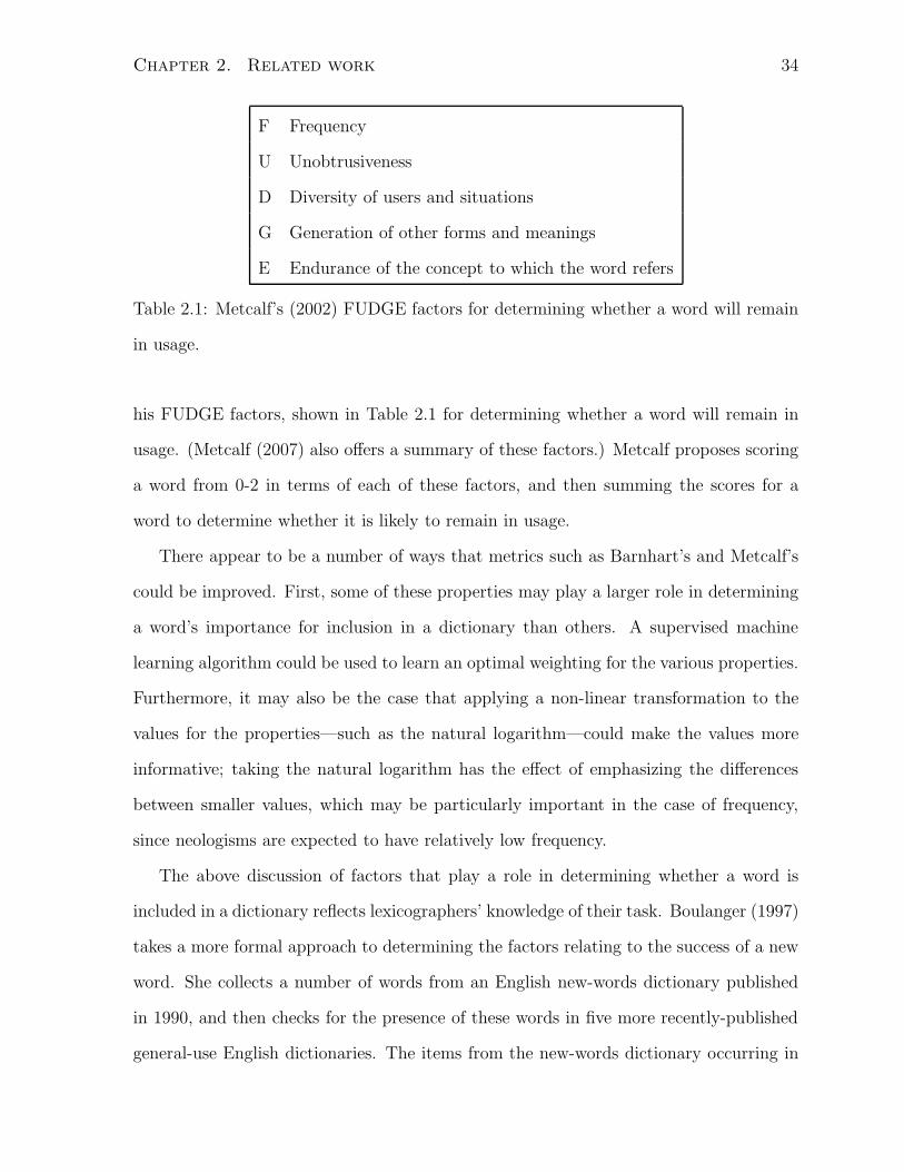
Chapter 2. Related work 34
F Frequency
U Unobtrusiveness
D Diversity of users and situations
G Generation of other forms and meanings
E Endurance of the concept to which the word refers
Table 2.1: Metcalf’s (2002) FUDGE factors for determining whether a word will remain
in usage.
his FUDGE factors, shown in Table 2.1 for determining whether a word will remain in
usage. (Metcalf (2007) also offers a summary of these factors.) Metcalf proposes scoring
a word from 0-2 in terms of each of these factors, and then summing the scores for a
word to determine whether it is likely to remain in usage.
There appear to be a number of ways that metrics such as Barnhart’s and Metcalf’s
could be improved. First, some of these properties may play a larger role in determining
a word’s importance for inclusion in a dictionary than others. A supervised machine
learning algorithm could be used to learn an optimal weighting for the various properties.
Furthermore, it may also be the case that applying a non-linear transformation to the
values for the properties—such as the natural logarithm—could make the values more
informative; taking the natural logarithm has the effect of emphasizing the differences
between smaller values, which may be particularly important in the case of frequency,
since neologisms are expected to have relatively low frequency.
The above discussion of factors that play a role in determining whether a word is
included in a dictionary reflects lexicographers’ knowledge of their task. Boulanger (1997)
takes a more formal approach to determining the factors relating to the success of a new
word. She collects a number of words from an English new-words dictionary published
in 1990, and then checks for the presence of these words in five more recently-published
general-use English dictionaries. The items from the new-words dictionary occurring in
Chapter 2. Related work 35
the general-use dictionaries are deemed successful new words that have been adopted into
general use; those that do not occur in the general-use dictionaries are assumed to be no
longer commonly used. Boulanger then compares a variety of properties of these words
across the two groups—successful and unsuccessful—to determine the factors affecting
the success of a new word.
A number of Boulanger’s findings are unsurprising given the above remarks by lexi-
cographers. Boulanger finds that frequent words are more likely to be successful, as are
words that are used in a non-specialized register. Furthermore, words for referents that
remained popular until the time of Boulanger’s study were also found to be more likely
to succeed than words whose referents were no longer popular at that time.
Interestingly, Boulanger finds that words associated with particular notional fields
(e.g., disease, economics) are more likely to succeed than others. This may seem some-
what contradictory to the observation by lexicographers that occurring across a variety of
genres and domains is an indication that a word is a good candidate for inclusion in a dic-
tionary. However, it has also been observed that the new words from a particular period
of time tend to reflect what was culturally prominent then (e.g., Ayto, 2006). Therefore,
association with a culturally prominent notional field appears to have a positive effect
on a word’s success.
Two of Boulanger’s findings have not been mentioned by any of the studies examined
so far in this thesis. She finds that new words which are in competition with an already
established word (i.e., the new word and established word are roughly synonymous) are
more likely to succeed than new words which are not in competition with an established
form. Boulanger hypothesizes that in the case of competition, only the new word itself
(i.e., the word form) must be accepted by speakers. In the no-competition case, both
the new word and new referent must be accepted. Boulanger also finds that taboo
association is related to the success of a word. She suggests that since taboo association
encourages lexical loss, this then encourages the formation of a new word to take its place.
Chapter 2. Related work 36
This is also discussed by Allan and Burridge (1991) in their treatment of euphemism
and dysphemism. A euphemistic term for a taboo subject may become contaminated
by its association with that subject, eventually losing its euphemistic status, thereby
encouraging the emergence of a new euphemistic term for that taboo subject.
One drawback to Boulanger’s study is that it does not directly consider whether a
new word has become successful. Instead, it examines whether a lexicographer considers
a new word to be worthy of inclusion in a dictionary. To the extent that lexicographers do
their jobs perfectly, and there is enough space in a dictionary to document all successful
neologisms, success and inclusion in a dictionary are the same. However, if lexicogra-
phers are making systematic errors, then the conclusions reached in this study relate to
properties of words that determine whether they will be listed in a dictionary, and not
whether they will become established in language. Nevertheless, it is not clear how such
a study could be conducted without making such an assumption.
A computational system for automatically identifying new words could exploit some of
the properties discussed in this section to rate whether a new word is worthy of inclusion in
a dictionary. Frequency information can be easily extracted from corpora, including range
(i.e., the number of documents in which a word occurs). Corpora which provide additional
information about the documents they include enable the extraction of properties such as,
for example, the number of genres in which a word occurs. Using automatic approaches
to stemming and lemmatization, it may also be possible to estimate the number of forms
of a new word. Corpora, such as the English Gigaword Corpus, consisting of newswire
stories over several years, could be used to estimate the time span over which a word
has been used. Unfortunately, it is currently unclear how properties of a word such as
the relevance of its referent, its cruciality in a language, and its obtrusiveness could be
automatically estimated.
Chapter 2. Related work 37
2.3.3 Finding new words
As discussed in Section 2.3.1.1, one way to find new words is by reading and looking
for them. As unsophisticated as this method may seem, the Oxford English Dictionary
still has a reading programme;5 as part of this process, volunteers read text and write
citations for interesting usages of new words that they find.
We also considered the use of electronic corpora for searching for citations for new
words in Section 2.3.1.2. If a lexicographer has a small amount of evidence for a word, or
a hunch that a word might be worth documenting, large corpora—in particular the World
Wide Web—are a potential source of more usages of that word. However, lexicographers
have noted a number of challenges to this, largely related to text normalization issues,
such as variant forms and spellings (e.g., Barnhart, 1985; Brookes, 2007). Nevertheless,
such problems are fairly straightforward to resolve through approaches to text normal-
ization (e.g., Sproat et al., 2001) which can be used, for example, to convert all instances
of a word in its various forms to a single canonical form. Barnhart (1985) also mentions
problems related to not knowing a word’s part-of-speech. For example, searching for
instances of the verb Google would be difficult, as this word is likely predominantly used
as a proper noun. However, this problem can be partially overcome by searching for
inflected forms of words (e.g., Googled). Moreover, approaches to part-of-speech tagging
(e.g., Brill, 1994; Mikheev, 1997) can automatically determine the syntactic category of
words.
Syntactic information may also be useful when searching for new words, and can be
automatically inferred—although noisily—using chunkers and parsers (e.g., Abney, 1991;
Collins, 2003). However, normalization problems are more difficult to resolve when using
the Web as a corpus due to the technical challenges of storing and processing very large
amounts of text. The Linguist’s Search Engine (Resnik et al., 2005) addressed many
5http://www.oed.com/readers/research.html
Chapter 2. Related work 38
of these issues and enabled linguistically-informed web queries including, for example,
searches for particular syntactic structures.
Lexicographers have noted that speakers and writers often use new words in a way
that indicates that they are new. Consider the following citation taken from The Double-
Tongued Dictionary :6
As material from the disk falls onto the surface of the pulsar, it imparts
enough angular momentum to spin back up into what scientists call a “recy-
cled pulsar.”
In this example, the newness of the word recycled pulsar is indicated by scare quotes
and the sequence of words what scientists call. McKean (2007) discusses conducting web
searches using particular phrases that are expected to be used with new words—such as
what scientists call—to identify new words. This is somewhat similar to computational
work that has made use of patterns to automatically extract hypernyms from corpora
(for example, using patterns such as NP1, NP2 and other NP3 to infer that NP3 is likely
a hypernym of NP1, Hearst, 1992). More recent computational work has considered
automatically learning the patterns that often express hypernymy (Snow et al., 2005).
So far, a similar study—learning the patterns that are likely to express new words—does
not appear to have been undertaken. A statistical analysis of the lexico-syntactic context
in which new words are used may reveal patterns in which new words are introduced;
these patterns could then be searched for on the Web, or in large corpora of recently-
produced text, to find new words.
This approach to finding new words is attractive in that it would be able to identify
both new word forms and new senses of existing words, as writers often use both in ways
that indicate that they are new. However, many of the words in The Double-Tongued
Dictionary appear to be technical terms from a specialized domain, such as recycled
6http://www.doubletongued.org
Chapter 2. Related work 39
pulsar above, that may in fact have been in use, although only by a small subset of
speakers, for quite some time. Nevertheless, considering our definition of neologism (see
Chapter 1, page 1), a word which has been used extensively but only in a particular
domain, and then becomes established in general usage, would indeed be a new word.
Moreover, after (automatically) finding a word that matches a pattern for new word
usage, we must also consider whether its other distributional properties as discussed in
Section 2.3.2—many of which can be automatically extracted—warrant its inclusion in
a dictionary.
O’Donovan and O’Neil (2008) describe the efforts of the lexicographers working on The
Chambers Dictionary to automatically identify neologisms. They maintain a reference
corpus of recent English which represents normal English usage. They then periodically
gather recent documents (from various sources on the Web and electronic editions of pub-
lications) which are then compared against the reference corpus. They identify all words
that do not already occur in their dictionary, and that have a frequency substantially
higher in the recent texts than in the reference corpus. Lexicographers then examine
these terms and consider them for inclusion as new dictionary entries.
This approach is somewhat limited in that it cannot identify new words that corre-
spond to multiword expressions (MWEs). This is especially problematic since many new
words are compounds (Algeo, 1991), which are often written as MWEs. Furthermore,
this method is generally not able to recognize neologisms that correspond to existing word
forms, however, O’Donovan and O’Neil are able to identify some shifts that correspond
to a change in syntactic category by finding usages of inflected forms.
The method of O’Donovan and O’Neil could potentially be improved to better identify
new meanings for existing word forms using more statistical distributional information
about the words under consideration. Lexico-syntactic information for each lemma in
the register corpus could be extracted; this could take the form of a word sketch, for
example. The same information could also be extracted for the lemmas in the new
Chapter 2. Related work 40
texts. Rather than compare the lemmas in the register corpus to those in the new
texts using simple frequency (as in O’Donovan and O’Neil, 2008), their word sketches
could instead be compared. The context in which a word is used—often as little as fifty
characters to the left and right—is usually sufficient to manually determine that word’s
sense (Moon, 1987). Indeed the assumption that context disambiguates has been widely
used in computational work on word sense disambiguation. Therefore, if the association
between a target word, and some other word in a particular syntactic relation, is found to
substantially differ between the register corpus and the new texts, this may be evidence of
a new sense of the target word. Novel MWEs that are sufficiently frequent in a collection
of new texts could be identified using statistics of association such as mutual information
(see Section 2.3.1.3). However, the frequency of many established MWEs is very low,
even in large corpora; therefore, even if we focus on documenting the more frequent new
MWEs, many of them can still be expected to have a low enough frequency that such
statistics will be unreliable. Nevertheless, approaches to identifying neologisms based
on their use in particular patterns that indicate the newness of a word—as discussed
above—appear to be applicable to MWEs and other low-frequency neologisms.
Chapter 3
Lexical blends
Lexical blends, also known as blends, are a common type of new word typically formed by
combining a prefix of one source word with a suffix of another source word, as in brunch
(breakfast and lunch). There may be overlap in the contribution of the source words,
as in fantabulous (fantastic and fabulous). It is also possible that one or both source
words are included in their entirety, for example, gaydar (gay radar) and jetiquette (jet
etiquette). We refer to blends such as these as simple two-word sequential blends, and
focus on this common type of blend in this chapter. Blends in which (part of) a word
is inserted within another (e.g., entertoyment, a blend of entertainment and toy) and
blends formed from more than two source words (e.g., nofriendo from no, friends, and
Nintendo) are rare. In Algeo’s (1991) study of new words, approximately 5% were blends
(see Table 1.1, page 8). However, in our analysis of 1,186 words taken from a popular
neologisms website, approximately 43% were blends. Clearly, computational techniques
are needed that can augment lexicons with knowledge of novel blends.
The precise nature and intended use of a computational lexicon will determine the
degree of processing required of a novel blend. In some cases it may suffice for the lexical
entry for a blend to simply consist of its source words. For example, a system that
employs a measure of distributional similarity may benefit from replacing occurrences
41
Chapter 3. Lexical blends 42
of a blend—likely a recently-coined and hence low frequency item—by its source words,
for which distributional information is likely available. In other cases, further semantic
reasoning about the blend and its source words may be required (e.g., determining the
semantic relationship between the source words as an approximation to the meaning of
the blend). However, any approach to handling blends will need to recognize that a
novel word is a blend and identify its source words. These two tasks are the focus of this
chapter. Specifically, we draw on linguistic knowledge of how blends are formed as the
basis for automatically determining the source words of a blend.
Language users create blends that tend to be interpretable by others. Tapping into
properties of blends believed to contribute to the recognizability of their source words—
and hence the interpretability of the resulting blend—we develop statistical measures
that indicate whether a candidate word pair is likely the source words for a given blend.
Moreover, the fact that a novel word is determined to have a “good” source word pair
may be evidence that it is in fact a blend, since we are unlikely to find two words that
are a “good” source word pair for a non-blend. Thus, the statistical measures we develop
for source word identification may also be useful in recognizing a novel word as a blend.
This chapter presents the first computational study of lexical blends. It was previ-
ously published by Cook and Stevenson (2010b), which is itself an extended and improved
version of the preliminary work done in this direction by Cook and Stevenson (2007).
Section 3.1 presents our statistical model for identifying a blend’s source words. We
describe our dataset of blends in Section 3.2, and the experimental setup in Section 3.3.
Results for the task of identifying a blend’s source words are given in Section 3.4. Sec-
tion 3.5 then gives preliminary results for distinguishing blends from other word types.
We discuss related work in Section 3.6, and summarize the contributions of this chapter
in Section 3.7.
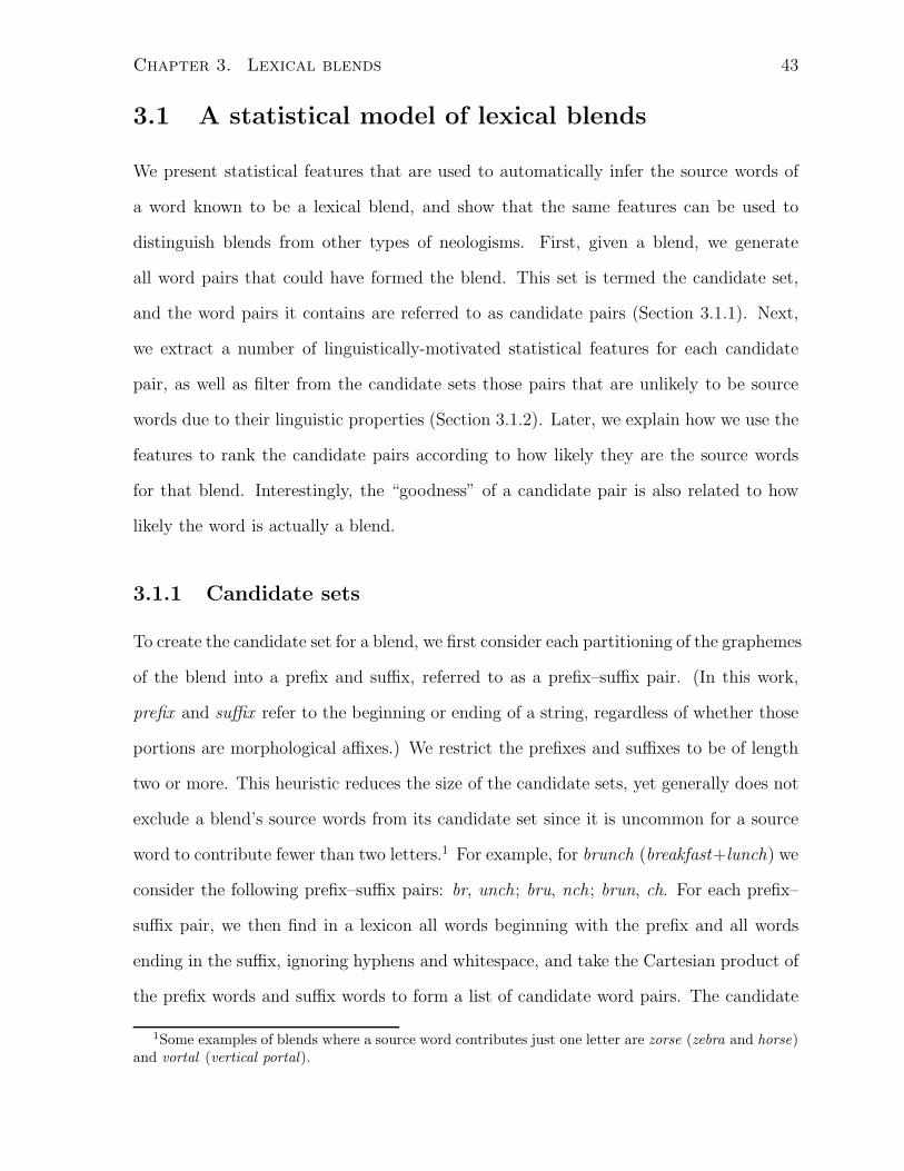
Chapter 3. Lexical blends 43
3.1 A statistical model of lexical blends
We present statistical features that are used to automatically infer the source words of
a word known to be a lexical blend, and show that the same features can be used to
distinguish blends from other types of neologisms. First, given a blend, we generate
all word pairs that could have formed the blend. This set is termed the candidate set,
and the word pairs it contains are referred to as candidate pairs (Section 3.1.1). Next,
we extract a number of linguistically-motivated statistical features for each candidate
pair, as well as filter from the candidate sets those pairs that are unlikely to be source
words due to their linguistic properties (Section 3.1.2). Later, we explain how we use the
features to rank the candidate pairs according to how likely they are the source words
for that blend. Interestingly, the “goodness” of a candidate pair is also related to how
likely the word is actually a blend.
3.1.1 Candidate sets
To create the candidate set for a blend, we first consider each partitioning of the graphemes
of the blend into a prefix and suffix, referred to as a prefix–suffix pair. (In this work,
prefix and suffix refer to the beginning or ending of a string, regardless of whether those
portions are morphological affixes.) We restrict the prefixes and suffixes to be of length
two or more. This heuristic reduces the size of the candidate sets, yet generally does not
exclude a blend’s source words from its candidate set since it is uncommon for a source
word to contribute fewer than two letters.1 For example, for brunch (breakfast+lunch) we
consider the following prefix–suffix pairs: br, unch; bru, nch; brun, ch. For each prefix–
suffix pair, we then find in a lexicon all words beginning with the prefix and all words
ending in the suffix, ignoring hyphens and whitespace, and take the Cartesian product of
the prefix words and suffix words to form a list of candidate word pairs. The candidate
1Some examples of blends where a source word contributes just one letter are zorse (zebra and horse)and vortal (vertical portal).
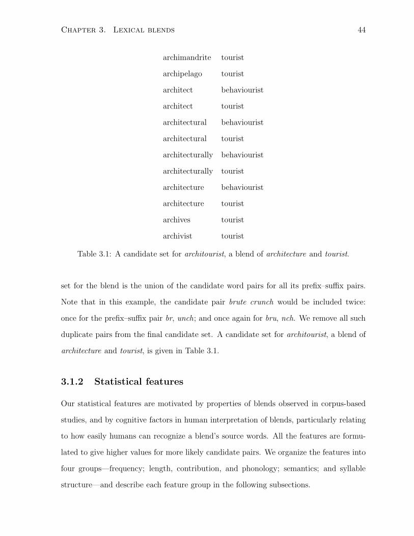
Chapter 3. Lexical blends 44
archimandrite tourist
archipelago tourist
architect behaviourist
architect tourist
architectural behaviourist
architectural tourist
architecturally behaviourist
architecturally tourist
architecture behaviourist
architecture tourist
archives tourist
archivist tourist
Table 3.1: A candidate set for architourist, a blend of architecture and tourist.
set for the blend is the union of the candidate word pairs for all its prefix–suffix pairs.
Note that in this example, the candidate pair brute crunch would be included twice:
once for the prefix–suffix pair br, unch; and once again for bru, nch. We remove all such
duplicate pairs from the final candidate set. A candidate set for architourist, a blend of
architecture and tourist, is given in Table 3.1.
3.1.2 Statistical features
Our statistical features are motivated by properties of blends observed in corpus-based
studies, and by cognitive factors in human interpretation of blends, particularly relating
to how easily humans can recognize a blend’s source words. All the features are formu-
lated to give higher values for more likely candidate pairs. We organize the features into
four groups—frequency; length, contribution, and phonology; semantics; and syllable
structure—and describe each feature group in the following subsections.
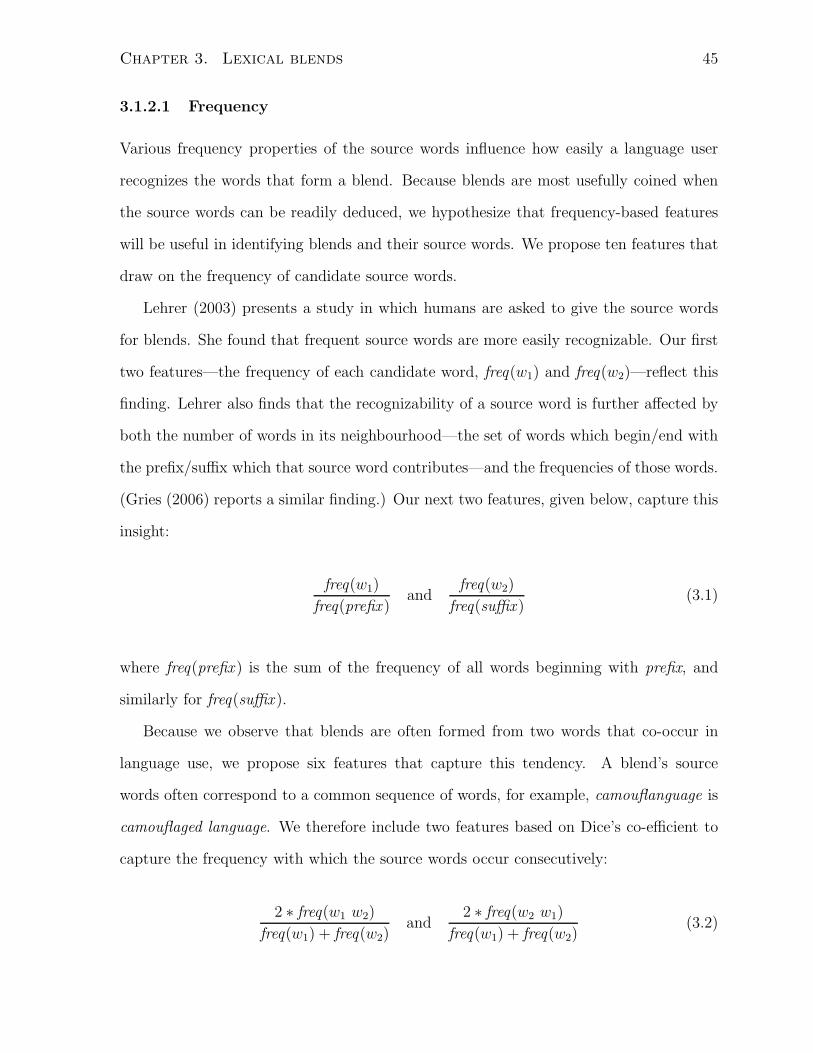
Chapter 3. Lexical blends 45
3.1.2.1 Frequency
Various frequency properties of the source words influence how easily a language user
recognizes the words that form a blend. Because blends are most usefully coined when
the source words can be readily deduced, we hypothesize that frequency-based features
will be useful in identifying blends and their source words. We propose ten features that
draw on the frequency of candidate source words.
Lehrer (2003) presents a study in which humans are asked to give the source words
for blends. She found that frequent source words are more easily recognizable. Our first
two features—the frequency of each candidate word, freq(w1) and freq(w2)—reflect this
finding. Lehrer also finds that the recognizability of a source word is further affected by
both the number of words in its neighbourhood—the set of words which begin/end with
the prefix/suffix which that source word contributes—and the frequencies of those words.
(Gries (2006) reports a similar finding.) Our next two features, given below, capture this
insight:
freq(w1)
freq(prefix )and
freq(w2)
freq(suffix )(3.1)
where freq(prefix ) is the sum of the frequency of all words beginning with prefix, and
similarly for freq(suffix ).
Because we observe that blends are often formed from two words that co-occur in
language use, we propose six features that capture this tendency. A blend’s source
words often correspond to a common sequence of words, for example, camouflanguage is
camouflaged language. We therefore include two features based on Dice’s co-efficient to
capture the frequency with which the source words occur consecutively:
2 ∗ freq(w1 w2)
freq(w1) + freq(w2)and
2 ∗ freq(w2 w1)
freq(w1) + freq(w2)(3.2)
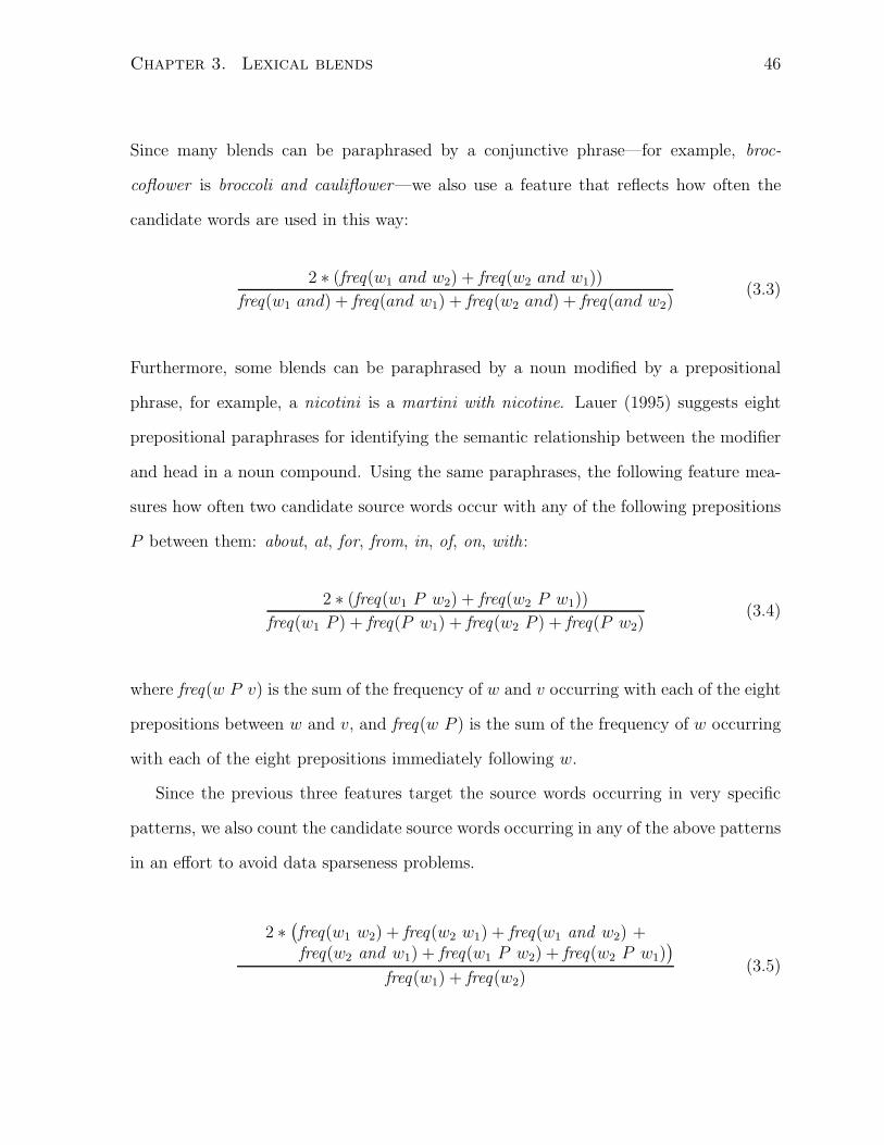
Chapter 3. Lexical blends 46
Since many blends can be paraphrased by a conjunctive phrase—for example, broc-
coflower is broccoli and cauliflower—we also use a feature that reflects how often the
candidate words are used in this way:
2 ∗ (freq(w1 and w2) + freq(w2 and w1))
freq(w1 and) + freq(and w1) + freq(w2 and) + freq(and w2)(3.3)
Furthermore, some blends can be paraphrased by a noun modified by a prepositional
phrase, for example, a nicotini is a martini with nicotine. Lauer (1995) suggests eight
prepositional paraphrases for identifying the semantic relationship between the modifier
and head in a noun compound. Using the same paraphrases, the following feature mea-
sures how often two candidate source words occur with any of the following prepositions
P between them: about, at, for, from, in, of, on, with:
2 ∗ (freq(w1 P w2) + freq(w2 P w1))
freq(w1 P ) + freq(P w1) + freq(w2 P ) + freq(P w2)(3.4)
where freq(w P v) is the sum of the frequency of w and v occurring with each of the eight
prepositions between w and v, and freq(w P ) is the sum of the frequency of w occurring
with each of the eight prepositions immediately following w.
Since the previous three features target the source words occurring in very specific
patterns, we also count the candidate source words occurring in any of the above patterns
in an effort to avoid data sparseness problems.
2 ∗(
freq(w1 w2) + freq(w2 w1) + freq(w1 and w2) +freq(w2 and w1) + freq(w1 P w2) + freq(w2 P w1)
)
freq(w1) + freq(w2)(3.5)
Chapter 3. Lexical blends 47
Finally, since the above patterns are very specific, and do not capture general co-
occurrence information which may also be useful in identifying a blend’s source words,
we include the following feature which counts the candidate source words co-occurring
within a five-word window.
2 ∗ freq(w1, w2 in a 5-word window)
freq(w1) + freq(w2)(3.6)
3.1.2.2 Length, contribution, and phonology
Ten features tap into properties of the orthographic or phonetic composition of the source
words and blend. Note that although we use information about the phonological and/or
syllabic structure of the source words, we do not assume such knowledge for the blend
itself, since it is a neologism for which such lexical information is typically unavailable.
The first word in a conjunct tends to be shorter than the second, and this also seems
to be the case for the source words in blends (Kelly, 1998; Gries, 2004). The first three
features therefore capture this tendency based on the graphemic, phonemic, and syllabic
length of w2 relative to w1, respectively:
lengraphemes(w2)
lengraphemes(w1) + lengraphemes(w2)(3.7)
lenphonemes(w2)
lenphonemes(w1) + lenphonemes(w2)(3.8)
lensyllables(w2)
lensyllables(w1) + lensyllables(w2)(3.9)
A blend and its second source word also tend to be similar in length, possibly because,
similar to compounds, the second source word of a blend is often the head; therefore it is
this word that determines the overall phonological structure of the resulting blend (Kubo-
zono, 1990). The following feature captures this property using graphemic length as an
Chapter 3. Lexical blends 48
approximation to phonemic length, since as stated above, we assume no phonological
information about the blend b.
1 −|lengraphemes(b) − lengraphemes(w2)|
max(lengraphemes(b), lengraphemes(w2))(3.10)
We hypothesize that a candidate source word is more likely if it contributes more
graphemes to a blend. We use two ways to measure contribution in terms of graphemes:
contseq(w, b) is the length of the longest prefix/suffix of word w which blend b begins/ends
with, and cont lcs(w, b) is the longest common subsequence (LCS) of w and b. This yields
four features, two using cont seq and two using cont lcs :
contseq(w1, b)
lengraphemes(w1)and
cont seq(w2, b)
lengraphemes(w2)(3.11)
cont lcs(w1, b)
lengraphemes(w1)and
cont lcs(w2, b)
lengraphemes(w2)(3.12)
Note that for some blends, such as spamdex (spam index ), contseq and cont lcs will be
equal; however, this is not the case in general, as in the blend tomacco (tomato and
tobacco) in which tomato overlaps with the blend not only in its prefix toma, but also in
the final o.
In order to be recognizable in a blend, the shorter source word will tend to contribute
more graphemes or phonemes, relative to its length, than the longer source word (Gries,
2004). We formulate the following feature which is positive only when this is the case:
(
contseq(w1, b)
lengraphemes(w1)−
contseq(w2, b)
lengraphemes(w2)
)
∗
(
lengraphemes(w2) − lengraphemes(w1)
lengraphemes(w1) + lengraphemes(w2)
)
(3.13)
Chapter 3. Lexical blends 49
For this feature we don’t have strong motivation to choose one measure of contribution
over the other, and therefore use contseq , the simpler version of contribution.
Finally, the source words in a blend are often phonologically similar, as in sheeple
(sheep people); the following feature captures this (Gries, 2006):
LCS phonemes(w1, w2)
max(lenphonemes(w1), lenphonemesw2)(3.14)
3.1.2.3 Semantics
We include two semantic features that are based on Lehrer’s (2003) observation that
people can more easily identify the source words of a blend when there is a semantic
relation between them.
As noted, blends are often composed of two semantically similar words, reflecting
a conjunction of their concepts. For example, a pug and a beagle are both a kind of
dog, and can be combined to form the blend puggle. Similarly an exergame is a blend
of exercise and game, both of which are types of activity. Our first semantic feature
captures similarity using an ontological similarity measure, which is calculated over an
ontology populated with word frequencies from a corpus.
The source words of some blends are not semantically similar (in the sense of their
relative positions within an ontology), but are semantically related. For example, the
source words of slanguist—slang and linguist—are related in that slang is a type of
language and a linguist studies language. Our second semantic feature is a measure of
semantic relatedness using distributional similarity between word co-occurrence vectors.
The semantic features are described in more detail in Section 3.3.2.
Chapter 3. Lexical blends 50
3.1.2.4 Syllable structure
Kubozono (1990) notes that the split of a source word—into the prefix/suffix it con-
tributes to the blend and the remainder of the word—occurs at a syllable boundary or
immediately after the onset of the syllable. Because this syllable structure property holds
sufficiently often, we use it as a filter over candidate pairs—rather than as an additional
statistical feature—in an effort to reduce the size of the candidate sets. Candidate sets
can be very large, and we expect that our features will be more successful at selecting the
correct source word pair from a smaller candidate set. In our results below, we analyze
the reduction in candidate set size using this syllable structure heuristic, and its impact
on performance.
3.2 Creating a dataset of recent blends
One potential source of a dataset of blends is the entries from a dictionary whose etymo-
logical entry indicates they were formed from a blend of two words. Using a dictionary
in this way provides an objective method for selecting experimental expressions and in-
dicating their gold standard source words. However, it results in a dataset of blends
that are sufficiently established in the language to appear in a dictionary. Truly novel
blends—neologisms which have been recently added to the language—may have differ-
ing properties from fully established forms in a dictionary. In particular, many of our
features are based on properties of the source words, both individually and in relation
to each other, that may not hold for expressions that entered the language some time
ago. For example, although meld is a blend of melt and weld, the current frequency of
the phrase melt and weld may not be as common as the source word co-occurrences for
newly-coined expressions. Thus, an important step to support further research on blends
is to develop a dataset of recent neologisms that are judged to be lexical blends.
To develop a dataset of recently-coined blends we drew on www.wordspy.com, a pop-
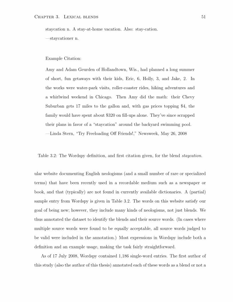
Chapter 3. Lexical blends 51
staycation n. A stay-at-home vacation. Also: stay-cation.
—staycationer n.
Example Citation:
Amy and Adam Geurden of Hollandtown, Wis., had planned a long summer
of short, fun getaways with their kids, Eric, 6, Holly, 3, and Jake, 2. In
the works were water-park visits, roller-coaster rides, hiking adventures and
a whirlwind weekend in Chicago. Then Amy did the math: their Chevy
Suburban gets 17 miles to the gallon and, with gas prices topping $4, the
family would have spent about $320 on fill-ups alone. They’ve since scrapped
their plans in favor of a “staycation” around the backyard swimming pool.
—Linda Stern, “Try Freeloading Off Friends!,” Newsweek, May 26, 2008
Table 3.2: The Wordspy definition, and first citation given, for the blend staycation.
ular website documenting English neologisms (and a small number of rare or specialized
terms) that have been recently used in a recordable medium such as a newspaper or
book, and that (typically) are not found in currently available dictionaries. A (partial)
sample entry from Wordspy is given in Table 3.2. The words on this website satisfy our
goal of being new; however, they include many kinds of neologisms, not just blends. We
thus annotated the dataset to identify the blends and their source words. (In cases where
multiple source words were found to be equally acceptable, all source words judged to
be valid were included in the annotation.) Most expressions in Wordspy include both a
definition and an example usage, making the task fairly straightforward.
As of 17 July 2008, Wordspy contained 1,186 single-word entries. The first author of
this study (also the author of this thesis) annotated each of these words as a blend or not a
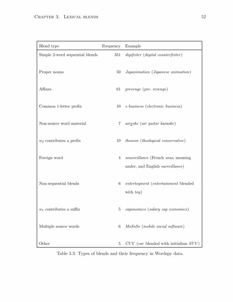
Chapter 3. Lexical blends 52
Blend type Frequency Example
Simple 2-word sequential blends 351 digifeiter (digital counterfeiter)
Proper nouns 50 Japanimation (Japanese animation)
Affixes 61 prevenge (pre- revenge)
Common 1-letter prefix 10 e-business (electronic business)
Non-source word material 7 aireoke (air guitar karaoke)
w2 contributes a prefix 10 theocon (theological conservative)
Foreign word 4 sousveillance (French sous, meaning
under, and English surveillance)
Non-sequential blends 6 entertoyment (entertainment blended
with toy)
w1 contributes a suffix 5 caponomics (salary cap economics)
Multiple source words 6 MoSoSo (mobile social software)
Other 5 CUV (car blended with initialism SUV )
Table 3.3: Types of blends and their frequency in Wordspy data.
Chapter 3. Lexical blends 53
blend, and indicated the source words for each blend. To ensure validity of the annotation
task, the second author similarly annotated 100 words randomly sampled from the 1,186.
On this subset of 100 words, observed agreement on both the blend/non-blend annotation
and the component source word identification was 92%, with an unweighted kappa score
of .84. On four blends, the annotators gave different variants of the same source word;
for example, fuzzy buzzword and fuzz buzzword for the blend fuzzword. These items were
counted as agreements, and all variants were considered correct source words.
Given the high level of agreement between the annotators, only one person annotated
all 1,186 items. 515 words were judged to be blends, with 351 being simple 2-word
sequential blends whose source words are not proper nouns (this latter type of blend
being the focus of this study). Table 3.3 shows the variety of blends encountered in the
Wordspy data, organized according to a categorization scheme we devised. Of the simple
2-word sequential blends, we restrict our experimental dataset to the 324 items whose
entries included a citation of their usage, as we have evidence that they have in fact been
used; moreover, such blends may be less likely to be nonce-formations—expressions which
are used once but do not become part of the language. The usage data in the citations
can also be used in the future for semantic features based on contextual information. We
refer to this new dataset of 324 items as Wordsplend (a blend of Wordspy and blend).
3.3 Materials and methods
3.3.1 Experimental expressions
The dataset used in the preliminary version of this study (Cook and Stevenson, 2007)
consisted of expressions from the Macquarie Dictionary (Delbridge, 1981) with an ety-
mology entry indicating that they are blends. All of our statistical features were devised
using the development portion of this dataset, enabling us to use the full Wordsplend
dataset for testing. To compare our current results to those in our preliminary study,
Chapter 3. Lexical blends 54
we also perform experiments on a subset of the Macquarie dataset. We are uncertain as
to whether a number of expressions indicated to be blends in the Macquarie Dictionary
are in fact blends. For example, it does not match our intuition that clash is a blend of
clap and dash. We created a second dataset of confirmed blends, Mac-Conf, consisting
of only those blends from Macquarie that are found in at least one of two additional
dictionaries with an etymology entry indicating that they are blends. We report results
on the 30 expressions in the unseen test portion of Mac-Conf.
3.3.2 Experimental resources
We generate candidate sets using two different lexicons: the CELEX lexicon (Baayen
et al., 1995),2 and a wordlist created from the Web 1T 5-gram Corpus (Brants and
Franz, 2006). These are discussed further just below. The frequency information needed
to calculate the frequency features is extracted from the Web 1T 5-gram Corpus. The
length, contribution, and phonology features, as well as the syllable structure filter, are
calculated on the basis of the source words themselves, or are derived from information in
CELEX (when CELEX is the lexicon in use).3 We compute semantic similarity between
the source words using Jiang and Conrath’s (1997) measure in the WordNet-Similarity
package (Pedersen et al., 2004), and we compute semantic relatedness of the pair using
the cosine between word co-occurrence vectors using software provided by Mohammad
and Hirst (2006).
We conduct separate experiments with the two different lexicons for candidate set
creation. We began by using CELEX, because it contains rich phonological information
that some of our features draw on. However, in our analysis of the results, we noted
2From CELEX, we use lemmas as potential source words, as it is uncommon for a source word to bean inflected form—there are no such examples in our development data.
3Note that it would be possible to automatically infer the phonological and syllabic informationrequired for our features using automatic approaches for text-to-phoneme conversion and syllabification(e.g., Bartlett et al., 2008). Although such techniques currently provide noisy information, phonologicaland syllabic information for the blend itself could also be inferred, allowing the development of featuresthat exploit this information. We leave exploring such possibilities for future work.
Chapter 3. Lexical blends 55
that for many expressions the correct candidate pair is not in the candidate set. Many
of the blends in Wordsplend are formed from words which are themselves new words,
often coined for concepts related to the Internet, such as download, for example; such
words are not listed in CELEX. This motivated us to create a lexicon from a recent
dataset (the Web 1T 5-gram Corpus) that would be expected to contain many of these
new coinages. To form a lexicon from this corpus, we extracted the 100K most frequent
words, restricted to lowercase and all-alphabetic forms. Using this lexicon we expect the
correct source word pair to be in the candidate set for more expressions. However, this
comes at the expense of potentially larger candidate sets, due to the larger lexicon size.
Furthermore, since this lexicon does not contain phonological or syllabic representations
of each word, we cannot extract three features: the feature for the syllable heuristic, and
the two features that capture the tendency for the second source word to be longer than
the first in terms of phonemes and syllables. (We do calculate the phonological similarity
between the two candidate source words, in terms of graphemes.)
3.3.3 Experimental methods
Since each of our features is designed to have a high value for a correct source word pair
and a low value otherwise, we can simply sum the features for each candidate pair to
get a score for each pair indicating its degree of goodness as a source word pair for the
blend under consideration. However, since our various features have values falling on
differing ranges, we first normalize the feature values by subtracting the mean of that
feature within that candidate set and dividing by the corresponding standard deviation.
We also take the arctan of each resulting feature value to reduce the influence of outliers.
We then sum the feature values for each candidate pair, and order the pairs within each
candidate set according to this sum. This ranks the pairs in terms of decreasing degree
of goodness as a source word pair. We refer to this method as the feature ranking
approach.
Chapter 3. Lexical blends 56
We also use a machine learning approach applied to the features in a training regimen.
Our task can be viewed as a classification problem in which each candidate pair is either
a positive instance (the correct source word pair) or a negative instance (an incorrect
source word pair). However, a standard machine learning algorithm does not directly
apply because of the structure of the problem space. In classification, we typically look for
a hyperplane that separates the positive and negative training examples. In the context
of our problem, this corresponds to separating all the correct candidate pairs (for all
blends in our dataset) from all the incorrect candidate pairs. However, such an approach
is undesirable as it ignores the structure of the candidate sets; it is only necessary to
separate the correct source word pair for a given blend from the corresponding incorrect
candidate pairs (i.e., for the same blend). This is also in line with the formulation of
our features, which are designed to give relatively higher values to correct candidate
pairs than incorrect candidate pairs within the candidate set for a given blend; it is not
necessarily the case that the feature values for the correct candidate pair for a given
blend will be higher than those for an incorrect candidate pair for another blend. In
other words, the features are designed to give values that are relative to the candidates
for a particular blend.
To address this issue, we use a version of the perceptron algorithm similar to that
proposed by Shen and Joshi (2005). In this approach, the classifier is trained by only ad-
justing the perceptron weight vector when the correct candidate pair is scored lower than
the incorrect pairs for the target blend (not across all the candidate pairs for all blends).
Furthermore, to accommodate the large variation in candidate set size, we use an uneven
margin—in this case the distance between the weighted sum of the feature vector for a
correct and incorrect candidate pair—of 1|correct cand. pairs|·|incorrect cand. pairs|
. We therefore
learn a single weight vector such that, within each candidate set, the correct candidate
pairs are scored higher than the incorrect candidate pairs by a factor of this margin.
When updating the weight vector, we multiply the update that we add to the weight
Chapter 3. Lexical blends 57
vector by a factor of this margin to prevent the classifier from being overly influenced
by large candidate sets. During testing, each candidate pair is ranked according to the
weighted sum of its feature vector. To evaluate this approach, on each of Wordsplend
and Mac-Conf we perform 10-fold cross-validation with 10 random restarts. In these
experiments, we use our syllable heuristic as a feature, rather than as a filter, to allow
the learner to weight it appropriately.
3.3.4 Evaluation metrics
We evaluate our methods according to two measures: accuracy and mean reciprocal rank
(MRR). Under the accuracy measure, the system is scored as correct if it ranks one of the
correct source word pairs for a given blend first, and as incorrect otherwise. The MRR
gives the mean of the rank of the highest ranked correct source word pair for each blend.
Although accuracy is more stringent than MRR, we are interested in MRR to see where
the system ranks the correct source word pair in the case that it is not ranked first.
We compare the accuracy of our system against two baselines. The chance (random)
baseline is the accuracy obtained by randomly selecting a candidate pair from the can-
didate set. We also consider an informed baseline in which the feature ranking approach
is applied using just two of our features, the frequency of each candidate source word.
3.4 Experimental results
3.4.1 Candidate sets
Recall that we construct candidate sets using two different resources, CELEX and the
Web 1T 5-gram Corpus. In Section 3.4.1.1 we examine some properties of the candidate
sets created using CELEX (also referred to as the CELEX candidate sets), and then in
Section 3.4.1.2 we consider the candidate sets built from the Web 1T 5-gram Corpus.
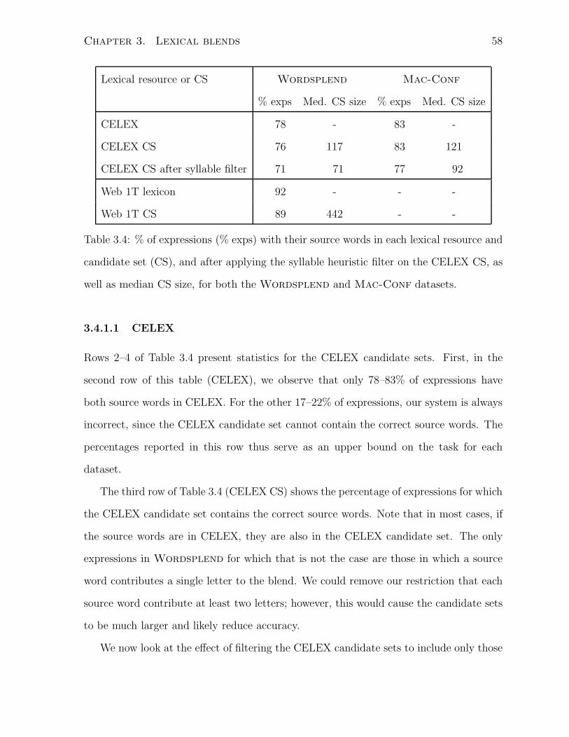
Chapter 3. Lexical blends 58
Lexical resource or CS Wordsplend Mac-Conf
% exps Med. CS size % exps Med. CS size
CELEX 78 - 83 -
CELEX CS 76 117 83 121
CELEX CS after syllable filter 71 71 77 92
Web 1T lexicon 92 - - -
Web 1T CS 89 442 - -
Table 3.4: % of expressions (% exps) with their source words in each lexical resource and
candidate set (CS), and after applying the syllable heuristic filter on the CELEX CS, as
well as median CS size, for both the Wordsplend and Mac-Conf datasets.
3.4.1.1 CELEX
Rows 2–4 of Table 3.4 present statistics for the CELEX candidate sets. First, in the
second row of this table (CELEX), we observe that only 78–83% of expressions have
both source words in CELEX. For the other 17–22% of expressions, our system is always
incorrect, since the CELEX candidate set cannot contain the correct source words. The
percentages reported in this row thus serve as an upper bound on the task for each
dataset.
The third row of Table 3.4 (CELEX CS) shows the percentage of expressions for which
the CELEX candidate set contains the correct source words. Note that in most cases, if
the source words are in CELEX, they are also in the CELEX candidate set. The only
expressions in Wordsplend for which that is not the case are those in which a source
word contributes a single letter to the blend. We could remove our restriction that each
source word contribute at least two letters; however, this would cause the candidate sets
to be much larger and likely reduce accuracy.
We now look at the effect of filtering the CELEX candidate sets to include only those
Chapter 3. Lexical blends 59
candidate pairs that are valid according to our syllable heuristic. This process results
in a 24–39% reduction in median candidate set size, but only excludes the source words
from the candidate set for a relatively small number of expressions (5–6%), as shown in
the fourth row of Table 3.4 (CELEX CS after syllable filter). We will further examine the
effectiveness of this heuristic when we consider the results for source word identification
in Section 3.4.2.
3.4.1.2 Web 1T 5-gram Corpus
Now we examine the candidate sets created using the lexicon derived from the Web 1T
5-gram Corpus.4 In the final two rows of Table 3.4 (Web 1T lexicon and Web 1T CS)
we see that, as expected, many more expressions have their source words in the Web 1T
lexicon than in CELEX, and furthermore, more expressions have their source words in
the candidate sets created using the Web 1T lexicon than in the candidate sets formed
from CELEX. This means that the upper bound for our task is much higher when using
the Web 1T lexicon than when using CELEX. However, this comes at the cost of creating
much larger candidate sets; we examine this trade-off more thoroughly below.
3.4.2 Source word identification
In the following subsections we present results using the feature ranking approach (Sec-
tion 3.4.2.1), and analyze some of the errors the system makes in these experiments
(Section 3.4.2.2). We then consider results using the modified perceptron algorithm
(Section 3.4.2.3), and finally we compare our results against those from our preliminary
study (Cook and Stevenson, 2007) and human performance (Section 3.4.2.4).
4Syllable structure information is not available for all words in the Web 1T lexicon, therefore we donot apply the syllable heuristic filter to the pairs in these candidate sets (see Section 3.3.2). We donot create candidate sets for Mac-Conf using the Web 1T lexicon since this lexicon was constructedspecifically in response to the kinds of new words found in Wordsplend.
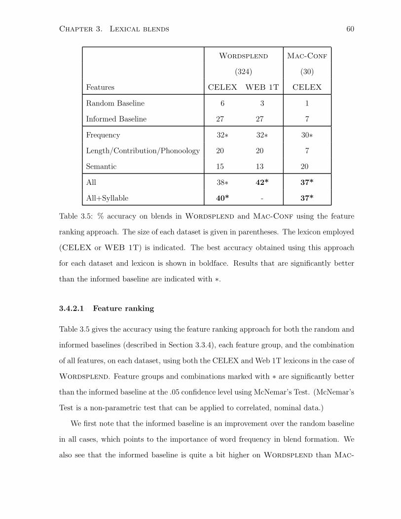
Chapter 3. Lexical blends 60
Wordsplend Mac-Conf
(324) (30)
Features CELEX WEB 1T CELEX
Random Baseline 6 3 1
Informed Baseline 27 27 7
Frequency 32∗ 32∗ 30∗
Length/Contribution/Phonoology 20 20 7
Semantic 15 13 20
All 38∗ 42* 37*
All+Syllable 40* - 37*
Table 3.5: % accuracy on blends in Wordsplend and Mac-Conf using the feature
ranking approach. The size of each dataset is given in parentheses. The lexicon employed
(CELEX or WEB 1T) is indicated. The best accuracy obtained using this approach
for each dataset and lexicon is shown in boldface. Results that are significantly better
than the informed baseline are indicated with ∗.
3.4.2.1 Feature ranking
Table 3.5 gives the accuracy using the feature ranking approach for both the random and
informed baselines (described in Section 3.3.4), each feature group, and the combination
of all features, on each dataset, using both the CELEX and Web 1T lexicons in the case of
Wordsplend. Feature groups and combinations marked with ∗ are significantly better
than the informed baseline at the .05 confidence level using McNemar’s Test. (McNemar’s
Test is a non-parametric test that can be applied to correlated, nominal data.)
We first note that the informed baseline is an improvement over the random baseline
in all cases, which points to the importance of word frequency in blend formation. We
also see that the informed baseline is quite a bit higher on Wordsplend than Mac-
Chapter 3. Lexical blends 61
Conf. Inspection of candidate sets—created from the CELEX lexicon—that include the
correct source words reveals that the average source word frequency for Wordsplend
is much higher than for Mac-Conf (118 million vs. 34 million). On the other hand, the
average for non-source words in the candidate sets is similar across these datasets (11M
vs. 9M). Thus, although source words are more frequent than non-source words for both
datasets, frequency is a much more reliable indicator of being a source word for truly
novel blends than for established blends. This finding emphasizes the need for a dataset
such as Wordsplend to evaluate methods for processing neologisms.
All of the individual feature groups outperform the random baseline. We also see
that our frequency features are better than the informed baseline. Although source word
frequency (the informed baseline) clearly plays an important role in forming interpretable
blends, this finding confirms that additional aspects of source word frequency beyond
their unigram counts also play an important role in blend formation. Also note that
the semantic features are substantially better than the informed baseline—although not
significantly so—on Mac-Conf, but not on Wordsplend. This result demonstrates
the importance of testing on true neologisms to have an accurate assessment of a method.
It also supports our future plan to explore alternative semantic features, such as those
that draw on the context of usage of a blend (as provided in Wordsplend).
We expect using all the features to give an improvement in performance over any
individual feature group, since they tap into very different types of information about
blends. Indeed the combination of all features (All) does perform better than the fre-
quency features, supporting our hypothesis that the information provided by the different
feature groups is complementary.5
Looking at the results on Wordsplend using the Web 1T lexicon, we see that as
expected, due to the larger candidate sets, the random baseline is lower than when using
5This difference is significant (p < 0.01) according to McNemar’s test for the Wordsplend datasetusing both the CELEX and Web 1T lexicons. The difference is not significant for Mac-Conf.
Chapter 3. Lexical blends 62
the CELEX lexicon. However, the informed baseline, and each feature group used on
its own, give very similar results, with only a small difference observed for the semantic
features. The combination of all features gives slightly higher performance using the Web
1T lexicon than the CELEX lexicon, although again this difference is rather small.
Recall that we wanted to see if the use of our syllable heuristic filter to reduce can-
didate set size would have a negative impact on performance. Table 3.5 shows that the
accuracy on all features when we apply our syllable heuristic filter (All+Syllable) is at
least as good as when we do not apply the filter (All). This is the case even though
the syllable heuristic filter removes the correct source word pairs for 5–6% of the blends
(see Table 3.4). It seems that the words this heuristic excludes from consideration are
not those that the features rank highly, indicating that it is a reasonable method for
pruning candidate sets. Moreover, reducing candidate set size will enable future work to
explore features that are more expensive to extract than those currently used. Given the
promising results using the Web1T lexicon, we also intend to examine ways to automat-
ically estimate the syllable filtering heuristic for words for which we do not have syllable
structure information.
3.4.2.2 Error analysis
We now examine some cases where the system ranks an incorrect candidate pair first, to
try to determine why the system makes the errors it does. We focus on the expressions in
Wordsplend using the CELEX lexicon, as we are able to extract all of our features for
this experimental setup. First, we observe that when considering feature groups individ-
ually, the frequency features perform best; however, in many cases, they also contribute
to errors. This seems to be primarily due to (incorrect) candidate pairs that occur very
frequently together. For example, in the case of mathlete (math athlete), the candidate
pair male athlete co-occurs much more frequently than the correct source word pair (math
athlete), causing the system to incorrectly rank the source word pair male athlete first.
Chapter 3. Lexical blends 63
We observe a similar situation for cutensil (cute utensil), where the candidate pair cup
and utensil often co-occur. In both these cases, phonological information for the blend
itself could help as, for example, cute ([kjut]) contributes more phonemes to cutensil
([kjutEnsl"]) than cup ([k2p]).
Turning to the length, contribution, and phonology features, we see that although
many blends exhibit the properties on which these features are based, there are also
many blends which do not. For example, our first feature in this group captures the
property that the second source word tends to be longer than the first; however, this
is not the case for some blends, such as testilie (testify and lie). Furthermore, even
for blends for which the second source word is longer than the first, there may exist
a candidate pair that has a higher value for this feature than the correct source word
pair. In the case of banalysis — banal analysis—banal electrolysis is a better source
word pair according to this feature. These observations, and similar issues with other
length, contribution, and phonology features, likely contribute to the poor performance
of this feature group. Moreover, such findings motivate approaches such as our modified
perceptron algorithm—discussed in the following subsection—that learn a weighting for
the features.
Finally, for the semantic features, we find cases where a blend’s source words are
similar and related, but there is another (incorrect) candidate pair which is more similar
and related according to these features. For example, puggle, a blend of pug and beagle,
has the candidate source words push and struggle which are more semantically similar
and related than the correct source word pair. In this case, the part-of-speech of the
candidate source words, along with contextual knowledge indicating the part-of-speech
of the blend, may be useful; blending pug and beagle would result in a noun, while a
blend of push and struggle would likely be a verb. Another example is camikini, a blend
of camisole and bikini. Both of these source words are women’s garments, so we would
expect them to have a moderately high similarity. However, the semantic similarity
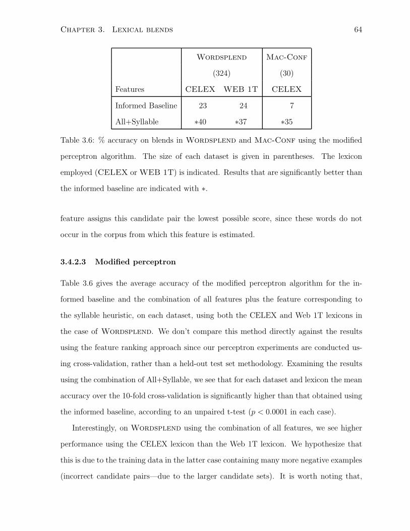
Chapter 3. Lexical blends 64
Wordsplend Mac-Conf
(324) (30)
Features CELEX WEB 1T CELEX
Informed Baseline 23 24 7
All+Syllable ∗40 ∗37 ∗35
Table 3.6: % accuracy on blends in Wordsplend and Mac-Conf using the modified
perceptron algorithm. The size of each dataset is given in parentheses. The lexicon
employed (CELEX or WEB 1T) is indicated. Results that are significantly better than
the informed baseline are indicated with ∗.
feature assigns this candidate pair the lowest possible score, since these words do not
occur in the corpus from which this feature is estimated.
3.4.2.3 Modified perceptron
Table 3.6 gives the average accuracy of the modified perceptron algorithm for the in-
formed baseline and the combination of all features plus the feature corresponding to
the syllable heuristic, on each dataset, using both the CELEX and Web 1T lexicons in
the case of Wordsplend. We don’t compare this method directly against the results
using the feature ranking approach since our perceptron experiments are conducted us-
ing cross-validation, rather than a held-out test set methodology. Examining the results
using the combination of All+Syllable, we see that for each dataset and lexicon the mean
accuracy over the 10-fold cross-validation is significantly higher than that obtained using
the informed baseline, according to an unpaired t-test (p < 0.0001 in each case).
Interestingly, on Wordsplend using the combination of all features, we see higher
performance using the CELEX lexicon than the Web 1T lexicon. We hypothesize that
this is due to the training data in the latter case containing many more negative examples
(incorrect candidate pairs—due to the larger candidate sets). It is worth noting that,
Chapter 3. Lexical blends 65
despite the differing experimental methodologies, the results are in fact not very different
from those obtained in the feature ranking approach. One limitation of this perceptron
algorithm is that it assumes that the training data is linearly separable. In future work,
we will try other machine learning techniques, such as that described by Joachims (2002),
that do not make this assumption.
3.4.2.4 Discussion
We now compare the feature ranking results on Mac-Conf here of 37% accuracy, to the
best results in our preliminary study on this dataset of 27% accuracy, also using feature
ranking (Cook and Stevenson, 2007) To make this comparison, we should consider the
differing baselines and upper bounds across the experiments. The informed baseline in
our preliminary study on Mac-Conf is 13%, substantially higher than the 7% in the
current study. Recall that the first row of Table 3.4 shows the upper bound using the
CELEX lexicon on this dataset to be 83%. By contrast, in our preliminary work we only
use blends whose source words appear in the lexicon we used there (Macquarie), so the
upper bound for that study is 100%. Taking these factors into account, the best results in
our preliminary study correspond to a reduction in error rate (RER) over the informed
baseline of 0.16, while the feature ranking method here using the combination of all
features and the syllable heuristic filter achieves a much higher RER of 0.39. (Reduction
in error rate = accuracy−baseline
upper bound−baseline.)
Lehrer (2003) finds human performance for determining the source words of blends
to be 34% to 79%—depending on the blends considered—which indicates the difficulty
of this task. (Note that the high level of interannotator agreement achieved in our
annotation task (Section 3.2) may seem surprising in the context of Lehrer’s results.
However, our task is much easier, since our annotators were given a definition of the
blend, while Lehrer’s subjects were not.) Our best accuracy on each dataset of 37%–42%
is quite respectable in comparison. These accuracies correspond to mean reciprocal ranks
Chapter 3. Lexical blends 66
of 0.47–0.51, while the random baseline on Wordsplend and Mac-Conf in terms of
this measure is 0.03–0.07. This indicates that even when our system is incorrect, the
correct source word pair is still ranked fairly high. Such information about the best
interpretations of a blend could be useful in semi-automated methods, such as computer-
aided translation, where a human may not be familiar with a novel blend in the source
text. Moreover, a list of possible interpretations for a blend—ranked by their likelihood—
could be more useful for NLP systems for tasks such as machine translation than a single
most likely interpretation.
3.5 Blend identification
The statistical features we have developed may also be informative about whether or not
a word is in fact a blend—that is, we expect that if a novel word has “good” candidate
source words, then the word is more likely to be a blend than the result of another word
formation process. Since our features are designed to be high for a blend’s source words
and low for other word pairs, we hypothesize that the highest scoring candidate pairs for
blends will be higher than those of non-blends.
To test this hypothesis, we first create a dataset of non-blends from our earlier annota-
tion, which found 671 non-blends out of the 1,186 Wordspy expressions (see Section 3.2).
From these words, we eliminate all those beginning with a capital letter (to exclude words
formed from proper nouns) or containing a non-letter character (to exclude acronyms and
initialisms). This results in 663 non-blends.
We create candidate sets for the non-blends using the CELEX lexicon. Using the
CELEX lexicon allows us to extract—and consider the contribution of—all of our length,
contribution, and phonology features, some of which are not available when using the Web
1T lexicon. The candidate sets resulting from using the CELEX lexicon were also much
smaller than when using the Web 1T lexicon. We calculate the features for the non-blends
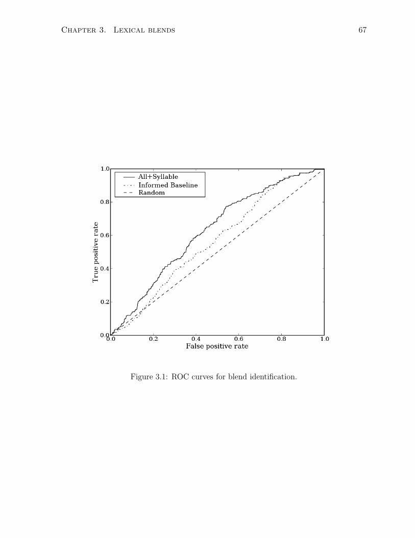
Chapter 3. Lexical blends 67
Figure 3.1: ROC curves for blend identification.
Chapter 3. Lexical blends 68
as we did for the blends, and then order all expressions (both blends and non-blends)
according to the sum of the features for their highest-scoring candidate source word pair.
We use the same feature groups and combinations presented in Table 3.5. Rather than
set an arbitrary cut-off to distinguish blends from non-blends, we instead give receiver
operating characteristic (ROC) curves for some of these experiments. ROC curves plot
true positive rate versus false positive rate as the cut-off is varied; see Figure 3.1. The
top-left corner represents perfect classification, with points further towards the top-left
from the diagonal (a random classifier) being “better.” We see that the informed baseline
is a substantial improvement over a random classifier, while the combination All+Syllable
is a further improvement over the informed baseline. The individual feature groups (not
shown in Figure 3.1) do not perform as well as All+Syllable. In future work, we plan to
re-examine this task and develop methods specifically for identifying blends and other
types of neologism.
3.6 Related Work
As discussed in Section 2.2, techniques generally used in the automatic acquisition of
syntactic and semantic properties of words are not applicable here, since they use corpus
statistics that cannot be accurately estimated for low-frequency items, such as the novel
lexical blends considered in this study (e.g., Hindle, 1990; Lapata and Brew, 2004; Joanis
et al., 2008). Other work that has used the context in which an unknown word occurs,
along with domain specific knowledge, to infer aspects of its meaning and syntax from
just one usage, or a small number of usages (e.g., Granger, 1977; Cardie, 1993; Hastings
and Lytinen, 1994), is also inapplicable; the domain-specific lexical resources that these
approaches rely on limit their applicability to general text.
Techniques for inferring lexical properties of neologisms can make use of information
that is typically not available in other lexical acquisition tasks—specifically, knowledge
Chapter 3. Lexical blends 69
of the processes through which neologisms are formed. Like the computational work
on neologisms discussed in Section 2.1 that concentrates on particular types of words,
this study also focuses on a specific word formation type, namely lexical blends. This
common word type has been unaddressed in computational linguistics except for our
previous work (Cook and Stevenson, 2007, 2010b).
In addition to knowledge about a word’s formation process, for many types of neolo-
gism, information about its phonological and orthographic content can be used to infer
aspects of its syntactic and semantic properties. This is the case for neologisms that are
composed of existing words or affixes (e.g., compounds and derivations) or partial ortho-
graphic or phonological material from existing words or affixes (e.g., acronyms, clippings,
and blends). For example, in the case of part-of-speech tagging, information about the
suffix of an unknown word can be used to determine its part-of-speech (e.g., Brill, 1994;
Ratnaparkhi, 1996; Mikheev, 1997, discussed in Section 2.1.1.1). For the task of inferring
the longform of an acronym, the letters which compose a given acronym can be used to
determine the most likely longform (e.g., Schwartz and Hearst, 2003; Nadeau and Turney,
2005; Okazaki and Ananiadou, 2006, discussed in Section 2.1.3.1).
The latter approach to acronyms is somewhat similar to the way in which we use
knowledge of the letters that make up a blend to form candidate sets and determine the
most likely source words. However, in the case of acronyms, each word in a longform
typically contributes only one letter to the acronym, while for blends, a source word
usually contributes more than one letter. At first glance, it may appear that this makes
the task of source word identification easier for blends, since there is more source word
material available to work with. However, acronyms have two properties that help in
their identification. First, there is less uncertainty in the “split” of an acronym, since
each letter is usually contributed by a separate word. By contrast, due to the large
variation in the amount of material contributed by the source words in blends, one
of the challenges in blend identification is to determine which material in the blend
Chapter 3. Lexical blends 70
belongs to each source word. Second, and more importantly, acronyms are typically
introduced in regular patterns (e.g., the longform followed by the acronym capitalized and
in parentheses) which can be exploited in acronym identification and longform inference;
in the case of blends there is no counterpart for this information.
3.7 Summary of contributions
This is the first computational study to consider lexical blends, a very frequent class
of new words. We propose a statistical model for inferring the source words of lexical
blends based largely on properties related to the recognizability of their source words.
We also introduce a method based on syllable structure for reducing the number of words
that are considered as possible source words. We evaluate our methods on two datasets,
one consisting of novel blends, the other containing established blends; in both cases
our features significantly outperform an informed baseline. We further show that our
methods for source word identification can also be used to distinguish blends from other
word types. We find evidence that blends tend to have candidate source word pairs
that are “good” according to our features while non-blends tend not to. In addition, we
annotate a dataset of newly-coined expressions which will support future research not
only on lexical blends, but on neologisms in general.
Chapter 4
Text message forms
Cell phone text messages—or SMS—contain many shortened and non-standard forms due
to a variety of factors, particularly the desire for rapid text entry (Grinter and Eldridge,
2001; Thurlow, 2003). Abbreviated forms may also be used because the number of
characters in a text message is sometimes limited to 160 characters, although this is
not always the case. Furthermore, text messages are written in an informal register;
non-standard forms are used to reflect this, and even for personal style (Thurlow, 2003).
These factors result in tremendous linguistic creativity, and hence many novel lexical
items, in the language of text messaging, or texting language.
One interesting consideration is whether text messaging and conventional writing con-
stitute two separate writing systems or variants of the same writing system. Sampson
(1985) claims that making distinctions between writing systems is as difficult as deter-
mining whether the speech of two communities corresponds to two different languages
or two dialects of the same language. Nevertheless, although we may not be able to
decisively answer this question, here we consider some of the differences between conven-
tional writing and text messaging from the perspective of writing systems. Logographs
are symbols which represent morphemes or words. English logographs include @ (at) and
& (and). Phonographs are symbols which represent sounds. The English writing system
71
Chapter 4. Text message forms 72
is largely phonographic. Logographs in conventional writing can be used as phonographs
in text messaging. For example, numerals are widely used phonographically in text mes-
saging forms, as in any1 (anyone) and b4 (before). Furthermore, in text messaging some
symbols can be used as word-level phonographs—e.g., r (are) and u (you)—but are not
typically used this way in conventional writing. Moreover, the use of logographs appears
to be more common in text messaging than in conventional writing. These differences
between conventional writing and text messaging pose difficulties for natural language
processing (NLP).
Normalization of non-standard forms is a challenge that must be tackled before other
types of NLP can take place (Sproat et al., 2001). In the case of text messages, text-
to-speech synthesis may be particularly useful for the visually impaired. For texting
language, given the abundance of creative forms, and the wide-ranging possibilities for
creating new forms, normalization is a particularly important problem, and has indeed
received some attention in computational linguistics (e.g., Aw et al., 2006; Choudhury
et al., 2007; Kobus et al., 2008; Yvon, 2010). Indeed, Aw et al. show that normal-
izing text messages prior to translation (to another language) can improve the quality
of the resulting translation, emphasizing the importance of methods for text message
normalization.
In this chapter we propose an unsupervised noisy channel method for texting lan-
guage normalization, that gives performance on par with that of a supervised system.
We use the term unsupervised here to mean specifically that our proposed method does
not rely directly on gold-standard training data, i.e., pairs of text messages and their
corresponding standard forms. We pursue unsupervised approaches to this problem, as
a large collection of gold-standard training data is not readily available. One notable ex-
ception is Fairon and Paumier (2006), although this resource is in French. (The resource
used in our study, provided by Choudhury et al. (2007), is quite small in comparison.)
Furthermore, other forms of computer-mediated communication, such as Internet mes-
Chapter 4. Text message forms 73
saging and microblogging, for example, Twitter,1 exhibit creative phenomena similar to
text messaging, although at a lower frequency (at least in the case of Internet messaging,
Ling and Baron, 2007). Moreover, technological changes, such as new input devices, are
likely to have an impact on the language of such media (Thurlow, 2003). On the other
hand, the rise of technology such as word prediction could reduce the use of abbreviations
in computer-mediated communication; however, it’s not clear such technology is widely
used (Grinter and Eldridge, 2001). An unsupervised approach, drawing on linguistic
properties of creative word formations, has the potential to be adapted for normalization
of text in other similar media—such as microblogging—without the cost of developing a
large training corpus. Moreover, normalization may be particularly important for such
media, given the need for applications such as translation and question answering.
We observe that many creative texting forms are the result of a small number of spe-
cific word formation processes. Rather than using a generic error model to capture all of
them, we propose a mixture model in which each word formation process is modeled ex-
plicitly according to linguistic observations specific to that formation. We do not consider
our method’s reliance on our observations about common word formation processes in
texting language to constitute a supervised approach—our method requires only general
observations about word formation processes and not specific gold-standard pairs of text
messages and their normalized forms. The remainder of this chapter is organized as fol-
lows: we present an analysis of a collection of texting forms in Section 4.1, which forms
the basis for the unsupervised model of text message normalization described in Sec-
tion 4.2. We discuss the experimental setup and system implementation in Section 4.3,
and present results in Section 4.4. Finally, we discuss related work in Section 4.5 and
summarize the contributions of this study in Section 4.6.
1http://twitter.com/
Chapter 4. Text message forms 74
4.1 Analysis of texting forms
To better understand the creative processes present in texting language, we categorize the
word formation process of each texting form in our development data, which consists of
400 texting forms paired with their standard forms.2 Several iterations of categorization
were done in order to determine sensible categories, and ensure categories were used
consistently. Since this data is only to be used to guide the construction of our system,
and not for formal evaluation, only one judge categorized the expressions (the author of
this thesis, a native English speaker). The findings are presented in Table 4.1.
Stylistic variations, by far the most frequent category, exhibit non-standard spelling,
such as representing sounds phonetically. Subsequence abbreviations, also very frequent,
are composed of a subsequence of the graphemes in a standard form, often omitting
vowels. These two formation types account for approximately 66% of our development
data; the remaining formation types are much less frequent. Suffix clippings and prefix
clippings consist of a prefix or suffix, respectively, of a standard form, and in some cases
a diminutive ending; we also consider clippings which omit just a final g (e.g., talkin) or
initial h (e.g., ello) from a standard form as they are rather frequent. (Thurlow (2003) also
observes an abundance of g-clippings.) A single letter or digit can be used to represent
a syllable; we refer to these as syllabic letter/digit. Phonetic abbreviations are variants
of clippings and subsequence abbreviations where some sounds in the standard form are
represented phonetically. Several texting forms appear to be spelling errors; we took the
layout of letters on cell phone keypads into account when making this judgement. The
items that did not fit within the above texting form categories were marked as unclear.
Finally, for some expressions the given standard form did not appear to be appropriate.
For example, gal is a colloquial English word meaning roughly the same as girl, but was
2Most texting forms have a unique standard form; however, some have multiple standard forms, e.g.,will and well can both be shortened to wl. In such cases we choose the word formation process throughwhich the texting form would be created from the most frequent standard form; in the case of frequencyties we choose arbitrarily among the categories corresponding to the most frequent standard forms.
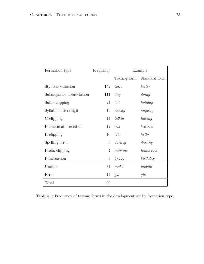
Chapter 4. Text message forms 75
Formation type Frequency Example
Texting form Standard form
Stylistic variation 152 betta better
Subsequence abbreviation 111 dng doing
Suffix clipping 24 hol holiday
Syllabic letter/digit 19 neway anyway
G-clipping 14 talkin talking
Phonetic abbreviation 12 cuz because
H-clipping 10 ello hello
Spelling error 5 darliog darling
Prefix clipping 4 morrow tomorrow
Punctuation 3 b/day birthday
Unclear 34 mobs mobile
Error 12 gal girl
Total 400
Table 4.1: Frequency of texting forms in the development set by formation type.
Chapter 4. Text message forms 76
annotated as a texting form of the standard form girl. Such cases were marked as errors.
No texting forms in our development data correspond to multiple standard form
words, for example, wanna for want to. (A small number of similar forms, however, ap-
pear with a single standard form word, and are marked as errors, e.g., the texting form
wanna annotated as the standard form want.) Acronyms and initialisms, such as LOL
and OMG, respectively, can also occur in text messaging, but are again very infrequent in
our development data. Previous approaches to text message normalization, such as Aw
et al. (2006) and Kobus et al. (2008), have considered issues related to texting forms cor-
responding to multiple standard forms. However, these approaches have limited means
for normalizing out-of-vocabulary texting forms. On the other hand, we focus specifi-
cally on creative formations in texting language. According to our development data,
such forms tend to have a one-to-one correspondence with a standard form. Moreover,
many texting forms which do correspond to multiple standard forms are well-established,
and could perhaps best be normalized through lexicon-based approaches. We therefore
assume that—for the purposes of this study—a texting form always corresponds to a
single standard form word.
It is important to note that some texting forms have properties of multiple categories,
for example, bak (back) could be considered a stylistic variation or a subsequence abbre-
viation. At this stage we are only trying to get a sense as to the common word formation
processes in texting language, and therefore in such cases we simply attempt to assign
the most appropriate category.
The design of our model for text message normalization, presented in the following
section, uses properties of the observed formation processes.
Chapter 4. Text message forms 77
4.2 An unsupervised noisy channel model for text
message normalization
Let S be a sentence consisting of standard forms s1s2...sn; in this study the standard
forms si are regular English words. Let T be a sequence of texting forms t1t2...tn, which
are the texting language realization of the standard form words, and may differ from the
standard forms. Given a sequence of texting forms T , the challenge is then to determine
the corresponding standard forms S.
Following Choudhury et al. (2007)—and various approaches to spelling error correc-
tion, such as, for example, Mays et al. (1991)—we model text message normalization
using a noisy channel. We want to find argmaxSP (S|T ). We apply Bayes rule and ig-
nore the constant term P (T ), giving argmaxSP (T |S)P (S). Making the independence
assumption that each texting form ti depends only on the standard form word si, and
not on the context in which it occurs, as in Choudhury et al., we express P (T |S) as a
product of probabilities: argmaxS (∏
i P (ti|si)) P (S).
We note in Section 4.1 that many texting forms are created through a small number
of specific word formation processes. Rather than model each of these processes at once
using a generic model for P (ti|si), as in Choudhury et al., we instead create several such
models, each corresponding to one of the observed common word formation processes.
We therefore rewrite P (ti|si) as∑
wf P (ti|si,wf )P (wf ) where wf is a word formation
process, e.g., subsequence abbreviation. Since, like Choudhury et al., we focus on the
word model, we simplify our model as below, to consider a single word si as opposed to
sequence of words S.
argmaxsi
∑
wf
P (ti|si,wf )P (wf )P (si)
We next explain the components of the model, P (ti|si,wf ), P (wf ), and P (si), referred
Chapter 4. Text message forms 78
to as the word model, word formation prior, and language model, respectively.
4.2.1 Word models
We now consider which of the word formation processes discussed in Section 4.1 to cap-
ture with a word model P (ti|si,wf ). Our choices here are based on the frequency of a
word formation process in the development data and how specific that process is. We
model stylistic variations and subsequence abbreviations simply due to their frequency.
We also choose to model suffix clippings since this word formation process is common
outside of text messaging (Kreidler, 1979; Algeo, 1991) and fairly frequent in our data.
Although g-clippings and h-clippings are moderately frequent, we do not model them,
as these very specific word formations are also (non-prototypical) subsequence abbrevi-
ations. The other less frequent formations—phonetic abbreviations, spelling errors, and
prefix clippings—are not modeled. On the one hand these word formation processes are
infrequent, and therefore modeling them explicitly is not expected to greatly improve
our system. On the other hand, these processes are somewhat similar to those we do
model, particularly stylistic variations. We therefore hypothesize that due to this simi-
larity the system will perform reasonably well on these word formation processes that are
not modeled. Syllabic letters and digits, or punctuation cannot be captured by any of
the word formation processes that we do model, and are therefore incorporated into our
model despite their low frequency in the development data. We capture these formations
heuristically by substituting digits with a graphemic representation (e.g., 4 is replaced
by for), and removing punctuation, before applying the model.
4.2.1.1 Stylistic variations
We propose a probabilistic version of edit-distance—referred to here as edit-probability—
inspired by Brill and Moore (2000) to model P (ti|si, stylistic variation). To compute
edit-probability, we consider the probability of each edit operation—substitution, inser-
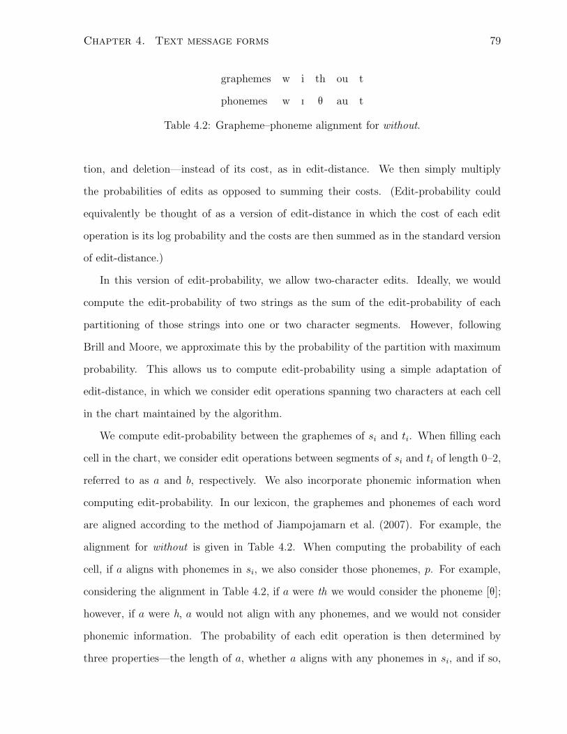
Chapter 4. Text message forms 79
graphemes w i th ou t
phonemes w I T au t
Table 4.2: Grapheme–phoneme alignment for without.
tion, and deletion—instead of its cost, as in edit-distance. We then simply multiply
the probabilities of edits as opposed to summing their costs. (Edit-probability could
equivalently be thought of as a version of edit-distance in which the cost of each edit
operation is its log probability and the costs are then summed as in the standard version
of edit-distance.)
In this version of edit-probability, we allow two-character edits. Ideally, we would
compute the edit-probability of two strings as the sum of the edit-probability of each
partitioning of those strings into one or two character segments. However, following
Brill and Moore, we approximate this by the probability of the partition with maximum
probability. This allows us to compute edit-probability using a simple adaptation of
edit-distance, in which we consider edit operations spanning two characters at each cell
in the chart maintained by the algorithm.
We compute edit-probability between the graphemes of si and ti. When filling each
cell in the chart, we consider edit operations between segments of si and ti of length 0–2,
referred to as a and b, respectively. We also incorporate phonemic information when
computing edit-probability. In our lexicon, the graphemes and phonemes of each word
are aligned according to the method of Jiampojamarn et al. (2007). For example, the
alignment for without is given in Table 4.2. When computing the probability of each
cell, if a aligns with phonemes in si, we also consider those phonemes, p. For example,
considering the alignment in Table 4.2, if a were th we would consider the phoneme [T];
however, if a were h, a would not align with any phonemes, and we would not consider
phonemic information. The probability of each edit operation is then determined by
three properties—the length of a, whether a aligns with any phonemes in si, and if so,
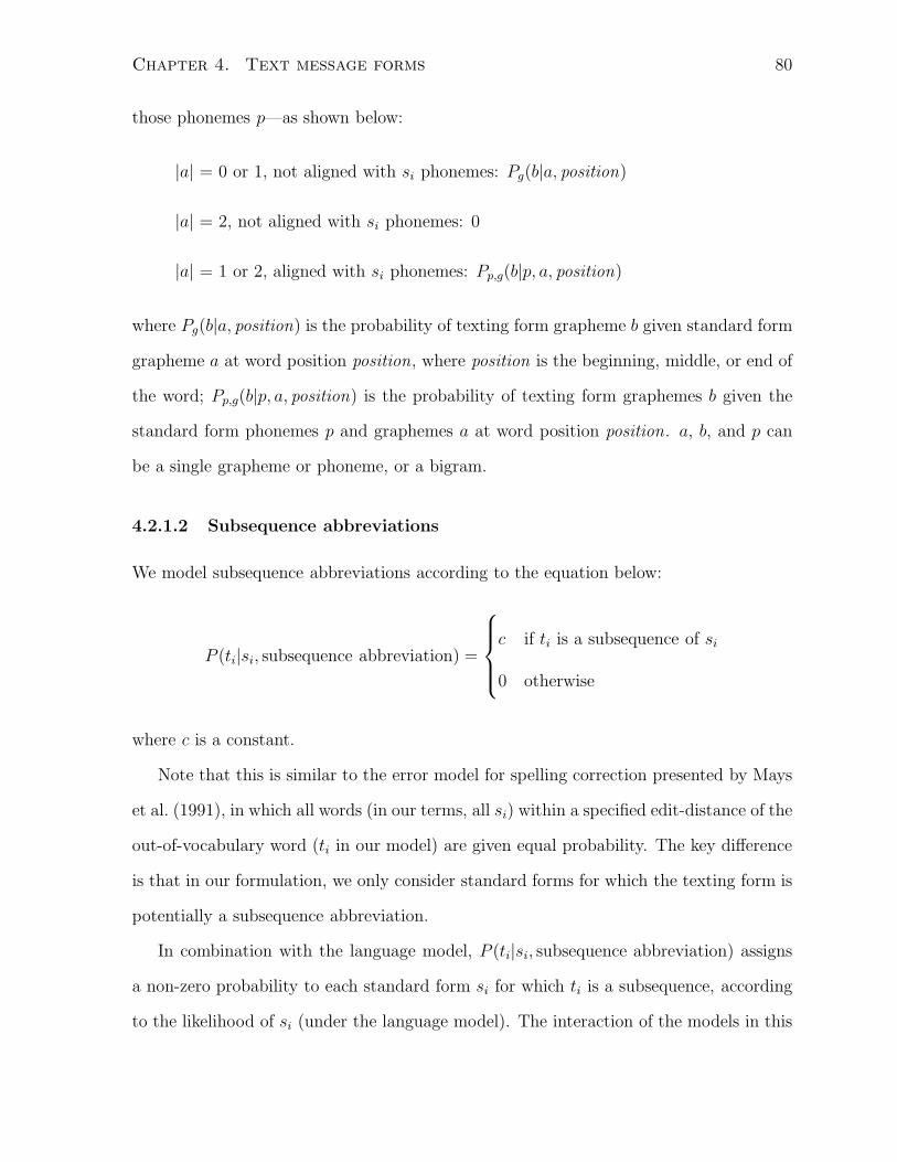
Chapter 4. Text message forms 80
those phonemes p—as shown below:
|a| = 0 or 1, not aligned with si phonemes: Pg(b|a, position)
|a| = 2, not aligned with si phonemes: 0
|a| = 1 or 2, aligned with si phonemes: Pp,g(b|p, a, position)
where Pg(b|a, position) is the probability of texting form grapheme b given standard form
grapheme a at word position position, where position is the beginning, middle, or end of
the word; Pp,g(b|p, a, position) is the probability of texting form graphemes b given the
standard form phonemes p and graphemes a at word position position. a, b, and p can
be a single grapheme or phoneme, or a bigram.
4.2.1.2 Subsequence abbreviations
We model subsequence abbreviations according to the equation below:
P (ti|si, subsequence abbreviation) =
c if ti is a subsequence of si
0 otherwise
where c is a constant.
Note that this is similar to the error model for spelling correction presented by Mays
et al. (1991), in which all words (in our terms, all si) within a specified edit-distance of the
out-of-vocabulary word (ti in our model) are given equal probability. The key difference
is that in our formulation, we only consider standard forms for which the texting form is
potentially a subsequence abbreviation.
In combination with the language model, P (ti|si, subsequence abbreviation) assigns
a non-zero probability to each standard form si for which ti is a subsequence, according
to the likelihood of si (under the language model). The interaction of the models in this
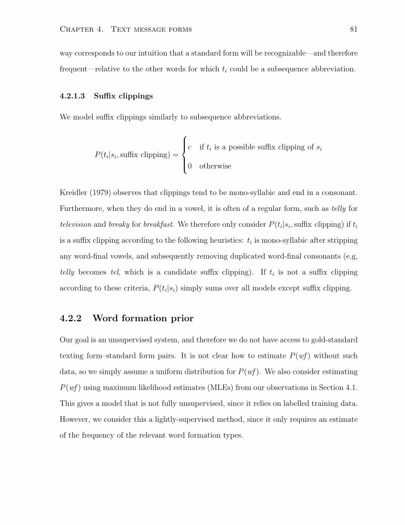
Chapter 4. Text message forms 81
way corresponds to our intuition that a standard form will be recognizable—and therefore
frequent—relative to the other words for which ti could be a subsequence abbreviation.
4.2.1.3 Suffix clippings
We model suffix clippings similarly to subsequence abbreviations.
P (ti|si, suffix clipping) =
c if ti is a possible suffix clipping of si
0 otherwise
Kreidler (1979) observes that clippings tend to be mono-syllabic and end in a consonant.
Furthermore, when they do end in a vowel, it is often of a regular form, such as telly for
television and breaky for breakfast. We therefore only consider P (ti|si, suffix clipping) if ti
is a suffix clipping according to the following heuristics: ti is mono-syllabic after stripping
any word-final vowels, and subsequently removing duplicated word-final consonants (e.g,
telly becomes tel, which is a candidate suffix clipping). If ti is not a suffix clipping
according to these criteria, P (ti|si) simply sums over all models except suffix clipping.
4.2.2 Word formation prior
Our goal is an unsupervised system, and therefore we do not have access to gold-standard
texting form–standard form pairs. It is not clear how to estimate P (wf ) without such
data, so we simply assume a uniform distribution for P (wf ). We also consider estimating
P (wf ) using maximum likelihood estimates (MLEs) from our observations in Section 4.1.
This gives a model that is not fully unsupervised, since it relies on labelled training data.
However, we consider this a lightly-supervised method, since it only requires an estimate
of the frequency of the relevant word formation types.
Chapter 4. Text message forms 82
4.2.3 Language model
Choudhury et al. (2007) find that using a bigram language model estimated over a bal-
anced corpus of English had a negative effect on their results compared with a unigram
language model, which they attribute to the unique characteristics of text messaging
that were not reflected in the corpus. We therefore use a unigram language model for
P (si), which also enables comparison with their results. Nevertheless, alternative lan-
guage models, such as higher order n-gram models, could easily be used in place of our
unigram language model.
4.3 Materials and methods
4.3.1 Datasets
We use the data provided by Choudhury et al. (2007) which consists of texting forms—
extracted from a collection of 900 text messages—and their manually determined stan-
dard forms. Our development data—used for model development and discussed in Sec-
tion 4.1—consists of the 400 texting form types that are not in Choudhury et al.’s held-out
test set, and that are not the same as one of their standard forms. The test data consists
of 1,213 texting forms and their corresponding standard forms. A subset of 303 of these
texting forms differ from their standard form.3 This subset is the focus of this study, but
we also report results on the full dataset.
3Choudhury et al. report that this dataset contains 1,228 texting forms. We found it to contain1,213 texting forms corresponding to 1,228 standard forms (recall that a texting form may have multiplestandard forms). There were similar inconsistencies with the subset of texting forms that differ fromtheir standard forms. Nevertheless, we do not expect these small differences to have an appreciable effecton the results.
Chapter 4. Text message forms 83
4.3.2 Lexicon
We construct a lexicon of potential standard forms such that it contains most words
that we expect to encounter in text messages, yet is not so large as to make it difficult
to identify the correct standard form. Our subjective analysis of the standard forms in
the development data is that they are frequent, non-specialized, words. To reflect this
observation, we create a lexicon consisting of all single-word entries containing only al-
phabetic characters found in both the CELEX Lexical Database (Baayen et al., 1995)
and the CMU Pronouncing Dictionary.4 We remove all words of length one (except a and
I ) to avoid choosing, for example, the letter r as the standard form for the texting form
r. We further limit the lexicon to words in the 20K most frequent alphabetic unigrams,
ignoring case, in the Web 1T 5-gram Corpus (Brants and Franz, 2006). The result-
ing lexicon contains approximately 14K words, and excludes only three of the standard
forms—cannot, email, and online—for the 400 development texting forms.
4.3.3 Model parameter estimation
MLEs for Pg(b|a, position)—needed to estimate P (ti|si, stylistic variation)—could be es-
timated from texting form–standard form pairs. However, since our system is unsuper-
vised, such data cannot be used. We therefore assume that many texting forms, and
other similar creative shortenings, occur on the web. We develop a number of character
substitution rules, for example, s⇒ z, and use them to create hypothetical texting forms
from standard words. We then compute MLEs for Pg(b|a, position) using the frequencies
of these derived forms on the web.
We create the substitution rules by examining examples in the development data,
considering fast speech variants and dialectal differences (e.g., voicing), and drawing on
our intuition. The derived forms are produced by applying the substitution rules to
4http://www.speech.cs.cmu.edu/cgi-bin/cmudict
Chapter 4. Text message forms 84
the words in our lexicon. To avoid considering forms that are themselves words, we
eliminate any form found in a list of approximately 480K words taken from SOWPODS
(the wordlist used in many Scrabble tournaments),5 and the Moby Word Lists.6 Finally,
we obtain the frequency of the derived forms from the Web 1T 5-gram Corpus.
To estimate Pp,g(b|p, a, position), we begin by first estimating two simpler distri-
butions: Ph(b|a, position) and Pp(b|p, position). Ph(b|a, position) is estimated in the
same manner as Pg(b|a, position), except that two-character substitutions are allowed.
Pp(b|p, position) is estimated from the frequency of p, and its alignment with b, in a
version of CELEX in which the graphemic and phonemic representation of each word is
many–many aligned using the method of Jiampojamarn et al. (2007).7 Pp,g(b|p, a, position)
is then an evenly-weighted linear combination of the estimates of this distribution us-
ing only graphemic and phonemic information, Ph(b|a, position) and Pp(b|p, position),
respectively. Finally, we smooth each of Pg(b|a, position) and Pp,g(b|p, a, position) using
add-alpha smoothing.
We set the constant c in our word models for subsequence abbreviations and suffix
clippings such that∑
siP (ti|si,wf )P (si) = 1. We similarly normalize the product of the
stylistic variation word model and the language model, P (ti|si, stylistic variation)P (si).8
We use the frequency of unigrams (ignoring case) in the Web 1T 5-gram Corpus to
estimate our language model. We expect the language of text messaging to be more
similar to that found on the web than that in a balanced corpus of English, such as the
British National Corpus (Burnard, 2007).
5http://en.wikipedia.org/wiki/SOWPODS6http://icon.shef.ac.uk/Moby/7We are very grateful to Sittichai Jiampojamarn for providing this alignment.8In our implementation of this model we in fact estimate P (si|ti,wf ) directly for subsequence ab-
breviations and suffix clippings rather than applying Bayes rule and calculating P (ti|si,wf )P (si). Thenormalization is necessary to account for the constant factor of P (ti) which is dropped from the denom-inator when Bayes rule is applied, but not when direct estimation is used. We present the model as inSection 4.2 to follow the presentation of previous models, such as Choudhury et al. (2007).
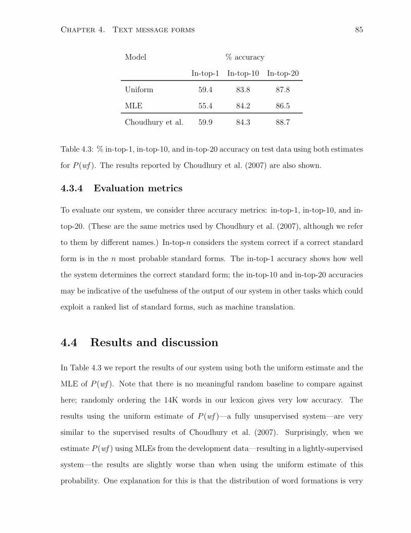
Chapter 4. Text message forms 85
Model % accuracy
In-top-1 In-top-10 In-top-20
Uniform 59.4 83.8 87.8
MLE 55.4 84.2 86.5
Choudhury et al. 59.9 84.3 88.7
Table 4.3: % in-top-1, in-top-10, and in-top-20 accuracy on test data using both estimates
for P (wf ). The results reported by Choudhury et al. (2007) are also shown.
4.3.4 Evaluation metrics
To evaluate our system, we consider three accuracy metrics: in-top-1, in-top-10, and in-
top-20. (These are the same metrics used by Choudhury et al. (2007), although we refer
to them by different names.) In-top-n considers the system correct if a correct standard
form is in the n most probable standard forms. The in-top-1 accuracy shows how well
the system determines the correct standard form; the in-top-10 and in-top-20 accuracies
may be indicative of the usefulness of the output of our system in other tasks which could
exploit a ranked list of standard forms, such as machine translation.
4.4 Results and discussion
In Table 4.3 we report the results of our system using both the uniform estimate and the
MLE of P (wf ). Note that there is no meaningful random baseline to compare against
here; randomly ordering the 14K words in our lexicon gives very low accuracy. The
results using the uniform estimate of P (wf )—a fully unsupervised system—are very
similar to the supervised results of Choudhury et al. (2007). Surprisingly, when we
estimate P (wf ) using MLEs from the development data—resulting in a lightly-supervised
system—the results are slightly worse than when using the uniform estimate of this
probability. One explanation for this is that the distribution of word formations is very
Chapter 4. Text message forms 86
different for the testing data and development data. However, we observe the same
difference in performance between the two approaches on the development data where
we expect to have an accurate MLE for P (wf ) (results not shown). We hypothesize that
the ambiguity of the categories of texting forms (see Section 4.1) results in poor MLEs
for P (wf ), thus making a uniform distribution, and hence fully-unsupervised approach,
more appropriate.
4.4.1 Results by formation type
We now consider in-top-1 accuracy for each word formation type, in Table 4.4. We
show results for the same word formation processes as in Table 4.1 (page 75), except
for h-clippings and punctuation, as no words of these categories are present in the test
data. We present results using the same experimental setup as before with a uniform
estimate of P (wf ) (All), and using just the model corresponding to the word formation
process (Specific), where applicable. (In this case our model then becomes, for each word
formation process wf , argmaxsiP (ti|si,wf )P (si).)
We first examine the top panel of Table 4.4 where we compare the performance on each
word formation type for both experimental conditions (Specific and All). We first note
that the performance using the formation-specific model on subsequence abbreviations
and suffix clippings is better than that of the overall model. This is unsurprising since we
expect that when we know a texting form’s formation process, and invoke a corresponding
specific model, our system should outperform a model designed to handle a range of
formation types. However, this is not the case for stylistic variations; here the overall
model performs better than the specific model. We observed in Section 4.1 that some
texting forms do not fit neatly into our categorization scheme; indeed, many stylistic
variations are also analyzable as subsequence abbreviations. Therefore, the subsequence
abbreviation model may improve normalization of stylistic variations. This model, used
in isolation on stylistic variations, gives an in-top-1 accuracy of 33.1%, indicating that
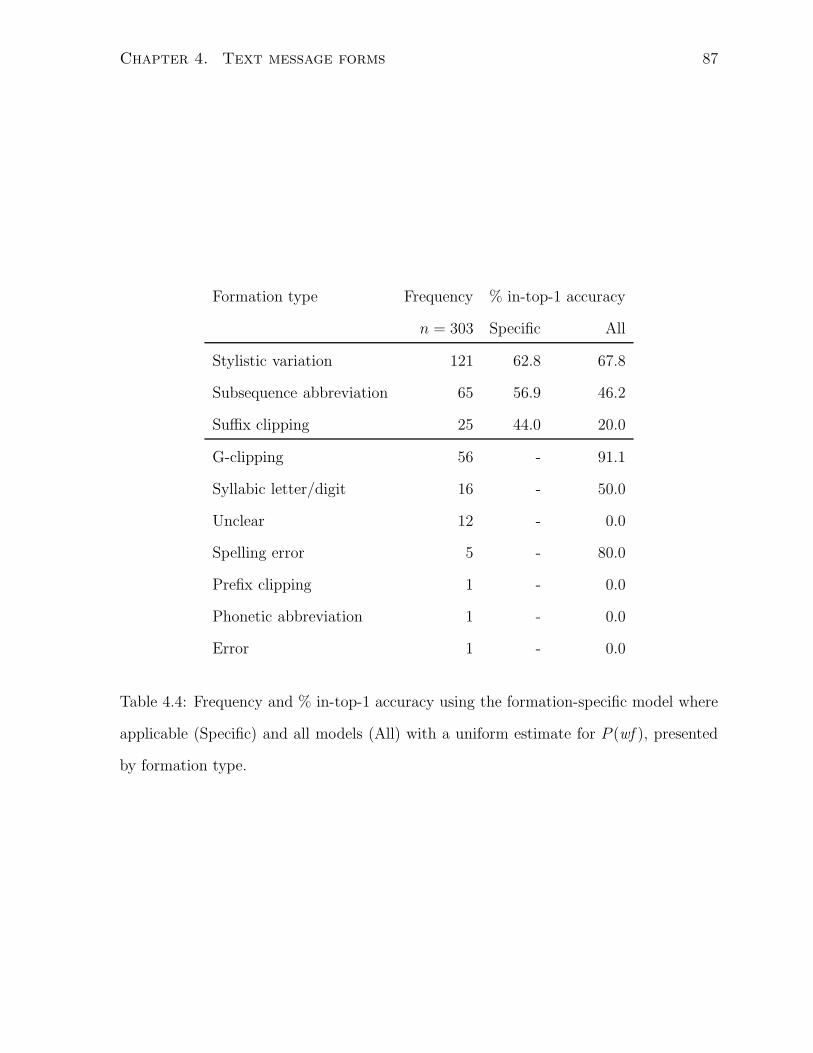
Chapter 4. Text message forms 87
Formation type Frequency % in-top-1 accuracy
n = 303 Specific All
Stylistic variation 121 62.8 67.8
Subsequence abbreviation 65 56.9 46.2
Suffix clipping 25 44.0 20.0
G-clipping 56 - 91.1
Syllabic letter/digit 16 - 50.0
Unclear 12 - 0.0
Spelling error 5 - 80.0
Prefix clipping 1 - 0.0
Phonetic abbreviation 1 - 0.0
Error 1 - 0.0
Table 4.4: Frequency and % in-top-1 accuracy using the formation-specific model where
applicable (Specific) and all models (All) with a uniform estimate for P (wf ), presented
by formation type.
Chapter 4. Text message forms 88
this may be the case.
Comparing the performance of the individual word models on only word types that
they were designed for (column Specific in Table 4.4), we see that the suffix clipping
model is by far the lowest, indicating that in the future we should consider ways of
improving this word model. One possibility is to incorporate phonemic knowledge. For
example, both friday and friend have the same probability under P (ti|si, suffix clipping)
for the texting form fri, which has the standard form friday in our data. (The language
model, however, does distinguish between these forms.) However, if we consider the
phonemic representations of these words, friday might emerge as more likely. Syllable
structure information may also be useful, as we hypothesize that clippings will tend to be
formed by truncating a word at a syllable boundary. We may similarly be able to improve
our estimate of P (ti|si, subsequence abbreviation). For example, for the texting form txt
both text and taxation have the same probability under this distribution, but intuitively
text, the correct standard form in our data, seems more likely. We could incorporate
knowledge about the likelihood of omitting specific characters, as in Choudhury et al.
(2007), to improve this estimate.
We now examine the lower panel of Table 4.4, in which we consider the performance
of the overall model on the word formation types that are not explicitly modeled. The
very high accuracy on g-clippings indicates that since these forms are also a type of
subsequence abbreviation, we do not need to construct a separate model for them. We
in fact also conducted experiments in which g-clippings and h-clippings were modeled
explicitly, but found these extra models to have little effect on the results.
Recall from Section 4.2.1 our hypothesis that prefix clippings, spelling errors, and
phonetic abbreviations have common properties with formation types that we do model,
and therefore the system will perform reasonably well on them. Here we find prelimi-
nary evidence to support this hypothesis as the accuracy on these three word formation
types (combined) is 57.1%. However, we must interpret this result cautiously as it only
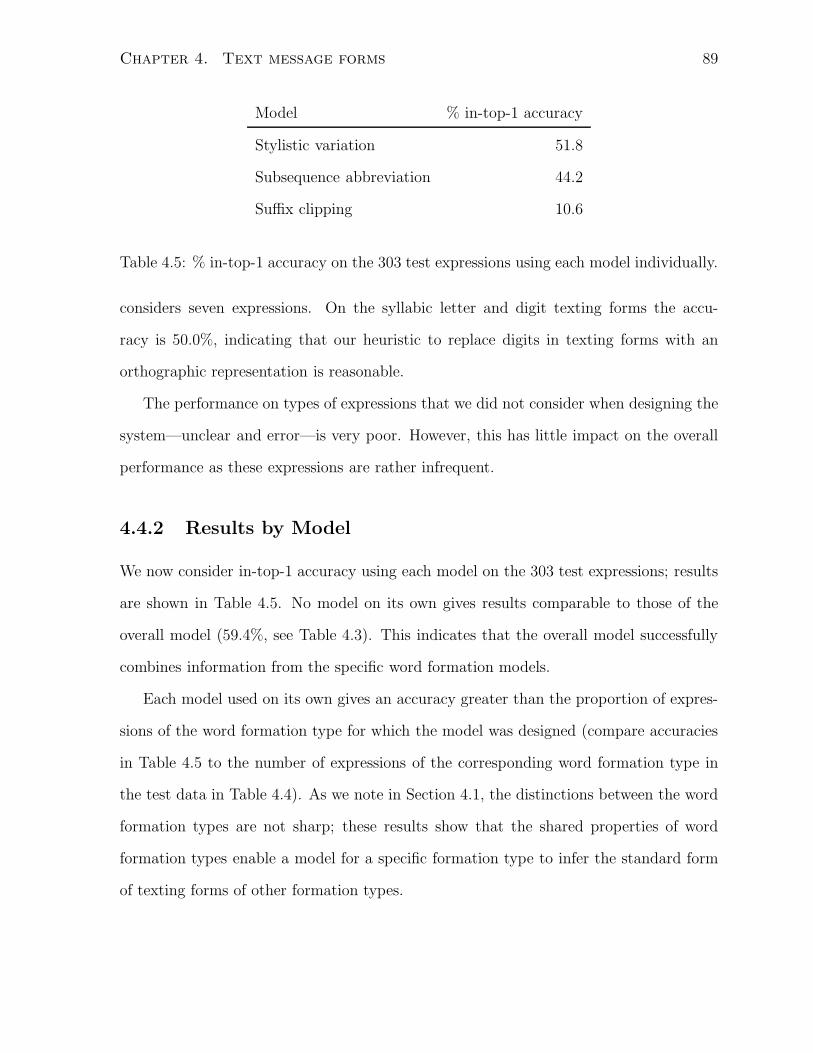
Chapter 4. Text message forms 89
Model % in-top-1 accuracy
Stylistic variation 51.8
Subsequence abbreviation 44.2
Suffix clipping 10.6
Table 4.5: % in-top-1 accuracy on the 303 test expressions using each model individually.
considers seven expressions. On the syllabic letter and digit texting forms the accu-
racy is 50.0%, indicating that our heuristic to replace digits in texting forms with an
orthographic representation is reasonable.
The performance on types of expressions that we did not consider when designing the
system—unclear and error—is very poor. However, this has little impact on the overall
performance as these expressions are rather infrequent.
4.4.2 Results by Model
We now consider in-top-1 accuracy using each model on the 303 test expressions; results
are shown in Table 4.5. No model on its own gives results comparable to those of the
overall model (59.4%, see Table 4.3). This indicates that the overall model successfully
combines information from the specific word formation models.
Each model used on its own gives an accuracy greater than the proportion of expres-
sions of the word formation type for which the model was designed (compare accuracies
in Table 4.5 to the number of expressions of the corresponding word formation type in
the test data in Table 4.4). As we note in Section 4.1, the distinctions between the word
formation types are not sharp; these results show that the shared properties of word
formation types enable a model for a specific formation type to infer the standard form
of texting forms of other formation types.
Chapter 4. Text message forms 90
4.4.3 All unseen data
Until now we have discussed results on our test data of 303 texting forms which differ
from their standard forms. We now consider the performance of our system on all 1,213
unseen texting forms, 910 of which are identical to their standard form. Since our model
was not designed with such expressions in mind, we slightly adapt it for this new task; if ti
is in our lexicon, we return that form as si, otherwise we apply our model as usual, using
the uniform estimate of P (wf ). This gives an in-top-1 accuracy of 88.2%, which is very
similar to the results of Choudhury et al. (2007) on this data of 89.1%. Note, however,
that Choudhury et al. only report results on this dataset using a uniform language model;9
since we use a unigram language model, it is difficult to draw firm conclusions about the
performance of our system relative to theirs.
4.5 Related Work
Aw et al. (2006) model text message normalization as translation from the texting lan-
guage into the standard language. Kobus et al. (2008) incorporate ideas from both
machine translation and automatic speech recognition for text message normalization.
However, both of the approaches of Aw et al. and Kobus et al. are supervised, and have
only limited means for normalizing texting forms that do not occur in the training data.
Yvon (2010) combines ideas from machine translation, automatic speech recognition,
and spelling error correction in his system for text message normalization, but again this
system is supervised.
The approach proposed in this chapter, like that of Choudhury et al. (2007), can be
viewed as a noisy-channel model for spelling error correction (e.g., Mays et al., 1991;
Brill and Moore, 2000), in which texting forms are seen as a kind of spelling error.
9Choudhury et al. do use a unigram language model for their experiments on the 303 texting formswhich differ from their standard forms (see Section 4.2.3).
Chapter 4. Text message forms 91
Furthermore, like our approach to text message normalization, approaches to spelling
correction have incorporated phonemic information (Toutanova and Moore, 2002).
The word model of the supervised approach of Choudhury et al. consists of hid-
den Markov models, which capture properties of texting language similar to those of
our stylistic variation model. We propose multiple word models—corresponding to fre-
quent texting language formation processes—and an unsupervised method for parameter
estimation.
4.6 Summary of contributions
We analyze a sample of text messaging forms to determine frequent word formation
processes in texting language. This analysis is revealing as to the range of creative
phenomena occurring in text messages.
Based on the above observations, we construct an unsupervised noisy-channel model
for text message normalization. On an unseen test set of 303 texting forms that differ
from their standard form, our model achieves 59% accuracy, which is on par with that
obtained by the supervised approach of Choudhury et al. (2007) on the same data.
Our approach is well-suited to normalization of novel creative texting forms—unlike
previously-proposed supervised approaches to text message normalization—and has the
potential to be applied to other domains, such as microblogging.
Chapter 5
Ameliorations and pejorations
Amelioration and pejoration are common linguistic processes through which the meaning
of a word changes to have a more positive or negative evaluation, respectively, in the mind
of the speaker. Historical examples of amelioration and pejoration include nice, which in
Middle English meant ‘foolish’, and vulgar, originally meaning ‘common’. More recent
examples are sick (now having a sense meaning ‘excellent’, an amelioration), and retarded
(now having a sense meaning ‘of inferior quality’, a pejoration, and often considered
offensive).
Amelioration and pejoration seem to come about in a number of ways, with these
processes taking place at the level of both concepts, and word forms or senses. If a
community’s evaluation of some concept changes, this may then result in amelioration or
pejoration. This seems to be the case with words such as authentic, local, and organic,
particularly when used to describe food, all of which are properties of foods which have
recently become highly valued by certain communities. In these cases the amelioration of
a particular concept (namely, authentic, local, and organic food) results in amelioration
of certain words.
A further possibility for amelioration or pejoration is that a word form acquires a new
sense. Gay (in its adjectival form) is one such example; in this case the primary sense
92
Chapter 5. Ameliorations and pejorations 93
of this word changed from ‘merry’ to ‘homosexual’, with the ‘merry’ sense being rather
uncommon nowadays. (More recently, gay has also come to be used in a sense—generally
considered offensive—meaning ‘of poor quality’.)
Pejoration in particular may also be caused by contamination through association
with a taboo concept. For example, toilet, as used in the phrase go to the toilet, was
originally a euphemistic borrowing from French (Allan and Burridge, 1991); however,
due to the taboo status of human waste it has lost its euphemistic status. Nowadays,
more euphemistic terms such as bathroom and loo are commonly used in American and
British English, respectively, in this context, and toilet has acquired a somewhat negative
status. In fact, euphemistic terms often become taboo terms—i.e., become pejorated—
due to their association with a taboo subject (Allan and Burridge, 1991). This example
with toilet also illustrates a related issue, namely, the potential lack of correspondence
between the evaluation of a word and the concept to which it refers. Although toilet
and bathroom both refer to the same physical place, toilet is somewhat more negative (in
contemporary Canadian usage). A similar situation is observed amongst near synonyms.
For example, lie and fib both refer to saying something that is not true, although lie is
much more negative than fib.
In the present study we consider amelioration and pejoration at the level of word
forms. Although it is certainly the case that concepts and particular word senses can
undergo amelioration and pejoration, we assume that these changes will be reflected in
the corresponding word forms.
Amelioration and pejoration are processes that change the semantic orientation of
a word, an aspect of lexical semantics that is of great interest nowadays. Much recent
computational work has looked at determining the sentiment or opinion expressed in
some text (see Pang and Lee, 2008, for an overview). A key aspect of many sentiment
analysis systems is a lexicon in which words or senses are annotated with semantic orien-
tation. Such lexicons are often manually-crafted (e.g., the General Inquirer, Stone et al.,
Chapter 5. Ameliorations and pejorations 94
1966). However, it is clearly important to have automatic methods to detect seman-
tic changes that affect a word’s orientation in order to keep such lexicons up-to-date,
whether automatically- or manually-created. Indeed, there have been recent efforts to
automatically infer polarity lexicons from corpora (e.g., Hatzivassiloglou and McKeown,
1997; Turney and Littman, 2003) and from other lexicons (e.g., Esuli and Sebastiani,
2006; Mohammad et al., 2009), and to adapt existing polarity lexicons to specific do-
mains (e.g., Choi and Cardie, 2009). Similarly, since appropriate usage of words depends
on knowledge of their semantic orientation, tools for detecting such changes would be
helpful for lexicographers in updating dictionaries.
Our hypothesis is that methods for automatically inferring polarity lexicons from
corpora can be used for detecting changes in semantic orientation, i.e., ameliorations
and pejorations. If the corpus-based polarity of a word is found to vary significantly
across two corpora which differ with respect to timespan, then that word is likely to
have undergone amelioration or pejoration. Moreover, this approach could be used to
find new word senses by applying it to corpora of recent text. Specifically, we adapt
an existing web-based method for calculating polarity (Turney and Littman, 2003) to
work on smaller corpora (since our corpora will be restricted by timespan), and apply
the method to words in the two corpora of interest.
5.1 Determining semantic orientation
Turney and Littman (2003) present web and corpus-based methods for determining the
semantic orientation of a target word. Their methods use either pointwise mutual infor-
mation (PMI) or latent semantic analysis (Deerwester et al., 1990) to compare a target
word to known words of positive and negative polarity. Here we focus on a variant of
their PMI-based method. In preliminary experiments we find a PMI-based method to
outperform a method using latent semantic analysis, and therefore choose to focus on
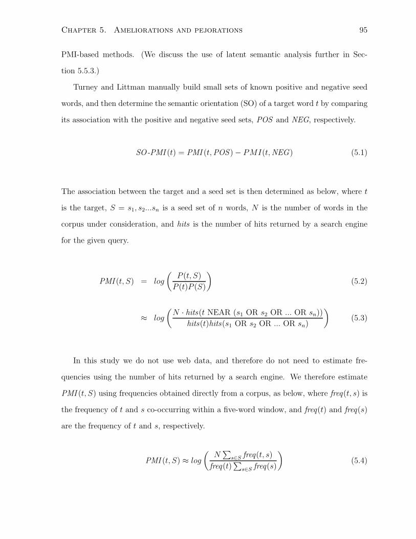
Chapter 5. Ameliorations and pejorations 95
PMI-based methods. (We discuss the use of latent semantic analysis further in Sec-
tion 5.5.3.)
Turney and Littman manually build small sets of known positive and negative seed
words, and then determine the semantic orientation (SO) of a target word t by comparing
its association with the positive and negative seed sets, POS and NEG, respectively.
SO-PMI (t) = PMI (t,POS) − PMI(t,NEG) (5.1)
The association between the target and a seed set is then determined as below, where t
is the target, S = s1, s2...sn is a seed set of n words, N is the number of words in the
corpus under consideration, and hits is the number of hits returned by a search engine
for the given query.
PMI (t, S) = log
(
P (t, S)
P (t)P (S)
)
(5.2)
≈ log
(
N · hits(t NEAR (s1 OR s2 OR ... OR sn))
hits(t)hits(s1 OR s2 OR ... OR sn)
)
(5.3)
In this study we do not use web data, and therefore do not need to estimate fre-
quencies using the number of hits returned by a search engine. We therefore estimate
PMI (t, S) using frequencies obtained directly from a corpus, as below, where freq(t, s) is
the frequency of t and s co-occurring within a five-word window, and freq(t) and freq(s)
are the frequency of t and s, respectively.
PMI (t, S) ≈ log
(
N∑
s∈S freq(t, s)
freq(t)∑
s∈S freq(s)
)
(5.4)
Chapter 5. Ameliorations and pejorations 96
We do not smooth these estimates. In this study, we only calculate the polarity of a word
t if it co-occurs at least five times with seed words—positive or negative—in the corpus
being used. Therefore the frequency of each word t is at least five so the denominator is
never zero. If t doesn’t co-occur with any seed word s ∈ S the numerator is zero, in which
case we simply set PMI (t, S) to a very low number (−∞). In this case t co-occurs at least
five times with the opposite seed set, and the resulting polarity is then the maximum
positive or negative polarity (∞ or −∞, respectively).
Turney and Littman focus on experiments using web data, the size of which allows
them to use very small, but reliable, seed sets of just seven words each. (Positive seeds:
good, nice, excellent, positive, fortunate, correct, superior ; negative seeds: bad, nasty,
poor, negative, unfortunate, wrong, inferior.) However, their small seed sets can cause
data sparseness problems when using the corpora of interest to us, which can be rather
small since they are restricted in time period. Therefore, we use the positive and negative
words from the General Inquirer (GI, Stone et al., 1966) as our seeds. Some words in
GI are listed with multiple senses, and the polarity of these senses may differ. To avoid
using seed words with ambiguous polarity, we select as seeds only those words which have
either positive or negative senses, but not both. This gives positive and negative seed sets
of 1621 and 1989 words, respectively, although at the cost of these seed words potentially
being less reliable indicators of polarity than those used by Turney and Littman. Note
that we obtain our seed words from a large manually-created lexicon, whereas Turney
and Littman use a much smaller amount of manual knowledge. This is a reflection of the
differing goals of our studies: Turney and Littman aim to automatically infer a polarity
lexicon similar to GI, whereas our goal is to use such a lexicon in order to identify
ameliorations and pejorations.
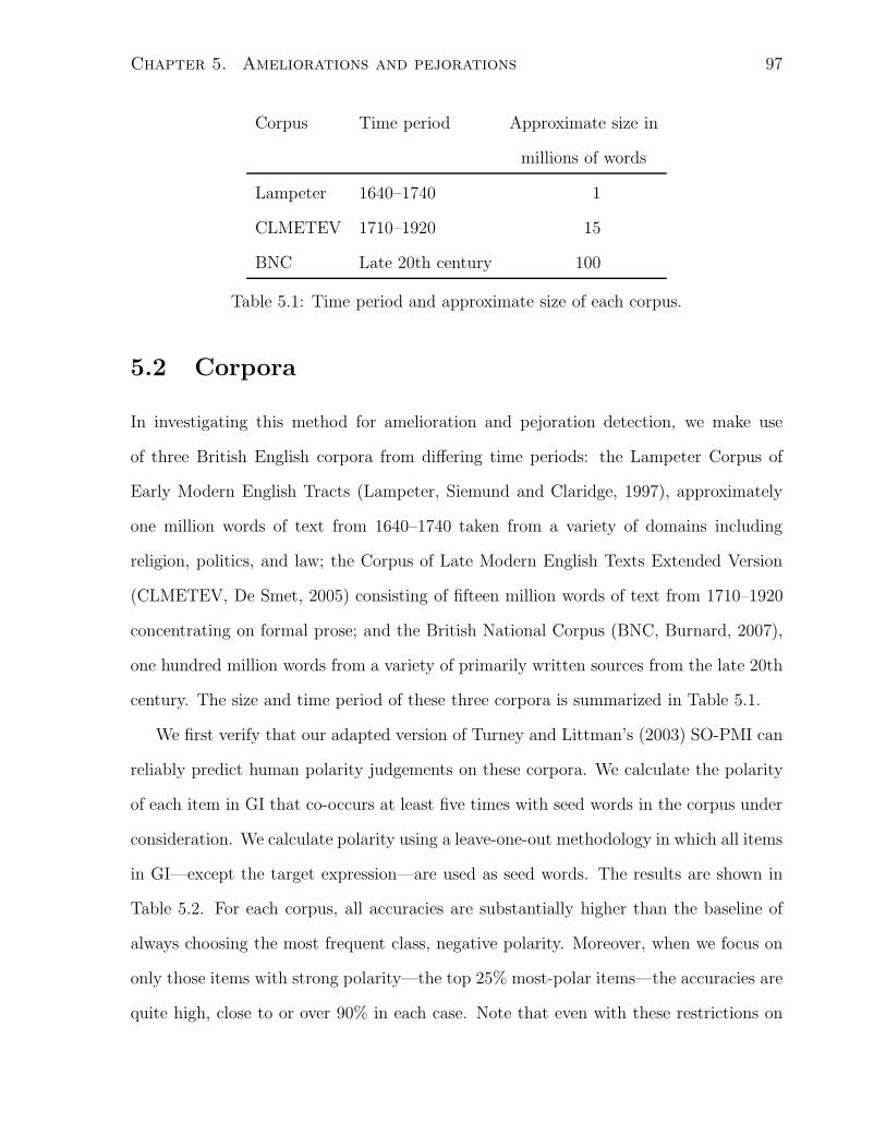
Chapter 5. Ameliorations and pejorations 97
Corpus Time period Approximate size in
millions of words
Lampeter 1640–1740 1
CLMETEV 1710–1920 15
BNC Late 20th century 100
Table 5.1: Time period and approximate size of each corpus.
5.2 Corpora
In investigating this method for amelioration and pejoration detection, we make use
of three British English corpora from differing time periods: the Lampeter Corpus of
Early Modern English Tracts (Lampeter, Siemund and Claridge, 1997), approximately
one million words of text from 1640–1740 taken from a variety of domains including
religion, politics, and law; the Corpus of Late Modern English Texts Extended Version
(CLMETEV, De Smet, 2005) consisting of fifteen million words of text from 1710–1920
concentrating on formal prose; and the British National Corpus (BNC, Burnard, 2007),
one hundred million words from a variety of primarily written sources from the late 20th
century. The size and time period of these three corpora is summarized in Table 5.1.
We first verify that our adapted version of Turney and Littman’s (2003) SO-PMI can
reliably predict human polarity judgements on these corpora. We calculate the polarity
of each item in GI that co-occurs at least five times with seed words in the corpus under
consideration. We calculate polarity using a leave-one-out methodology in which all items
in GI—except the target expression—are used as seed words. The results are shown in
Table 5.2. For each corpus, all accuracies are substantially higher than the baseline of
always choosing the most frequent class, negative polarity. Moreover, when we focus on
only those items with strong polarity—the top 25% most-polar items—the accuracies are
quite high, close to or over 90% in each case. Note that even with these restrictions on
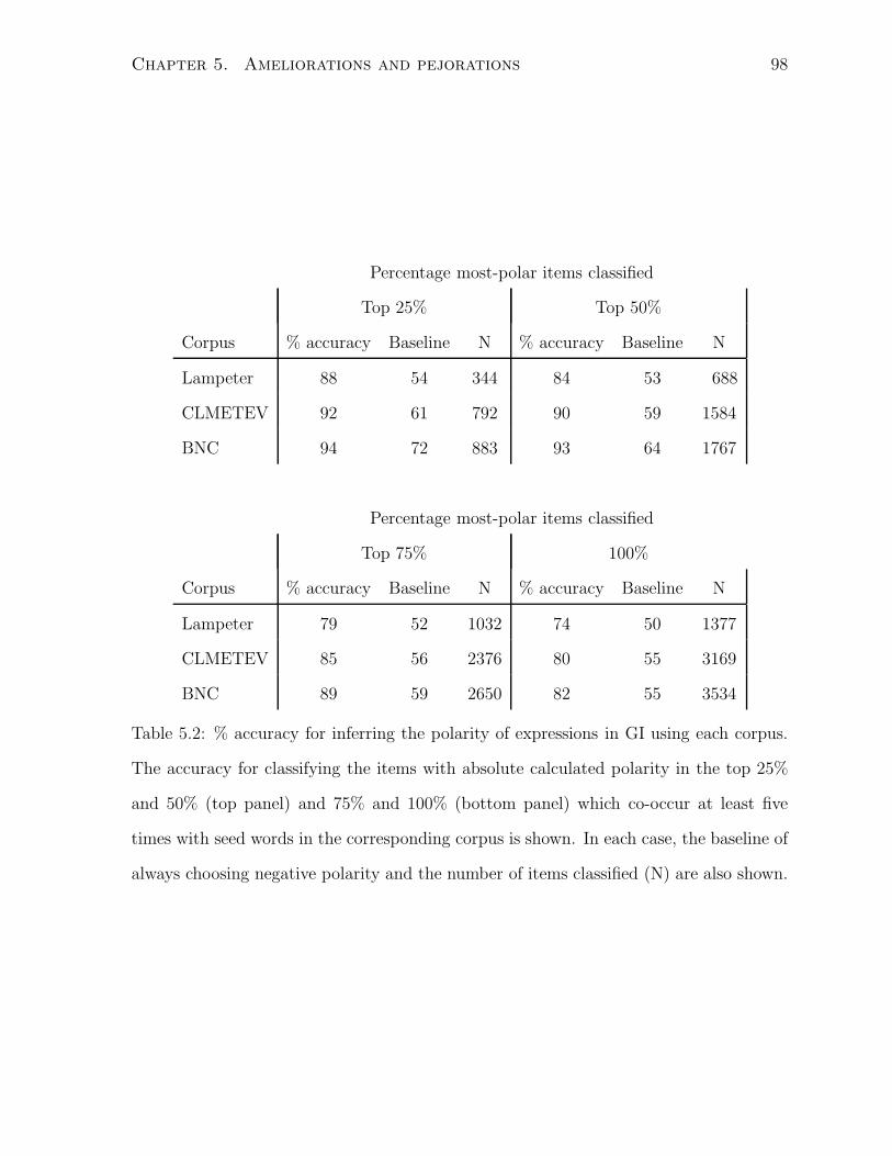
Chapter 5. Ameliorations and pejorations 98
Percentage most-polar items classified
Top 25% Top 50%
Corpus % accuracy Baseline N % accuracy Baseline N
Lampeter 88 54 344 84 53 688
CLMETEV 92 61 792 90 59 1584
BNC 94 72 883 93 64 1767
Percentage most-polar items classified
Top 75% 100%
Corpus % accuracy Baseline N % accuracy Baseline N
Lampeter 79 52 1032 74 50 1377
CLMETEV 85 56 2376 80 55 3169
BNC 89 59 2650 82 55 3534
Table 5.2: % accuracy for inferring the polarity of expressions in GI using each corpus.
The accuracy for classifying the items with absolute calculated polarity in the top 25%
and 50% (top panel) and 75% and 100% (bottom panel) which co-occur at least five
times with seed words in the corresponding corpus is shown. In each case, the baseline of
always choosing negative polarity and the number of items classified (N) are also shown.
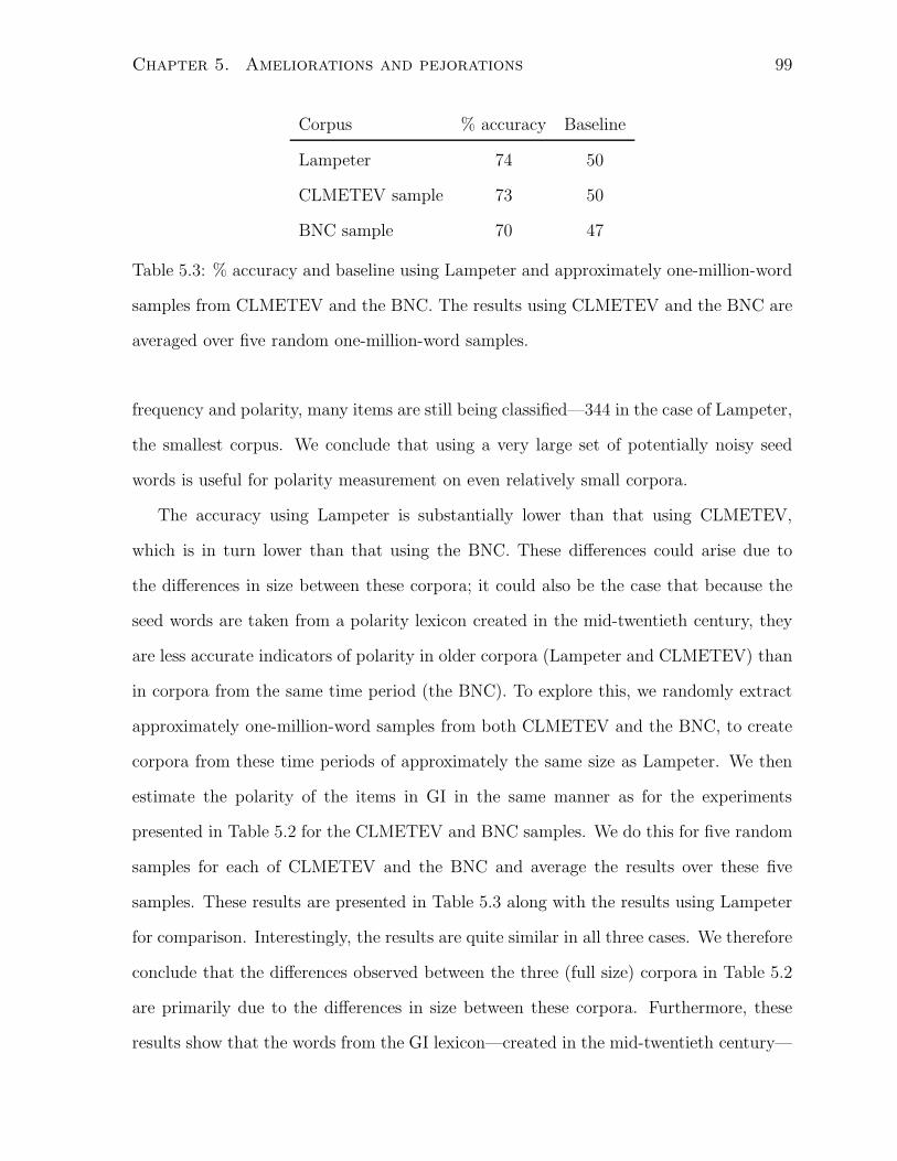
Chapter 5. Ameliorations and pejorations 99
Corpus % accuracy Baseline
Lampeter 74 50
CLMETEV sample 73 50
BNC sample 70 47
Table 5.3: % accuracy and baseline using Lampeter and approximately one-million-word
samples from CLMETEV and the BNC. The results using CLMETEV and the BNC are
averaged over five random one-million-word samples.
frequency and polarity, many items are still being classified—344 in the case of Lampeter,
the smallest corpus. We conclude that using a very large set of potentially noisy seed
words is useful for polarity measurement on even relatively small corpora.
The accuracy using Lampeter is substantially lower than that using CLMETEV,
which is in turn lower than that using the BNC. These differences could arise due to
the differences in size between these corpora; it could also be the case that because the
seed words are taken from a polarity lexicon created in the mid-twentieth century, they
are less accurate indicators of polarity in older corpora (Lampeter and CLMETEV) than
in corpora from the same time period (the BNC). To explore this, we randomly extract
approximately one-million-word samples from both CLMETEV and the BNC, to create
corpora from these time periods of approximately the same size as Lampeter. We then
estimate the polarity of the items in GI in the same manner as for the experiments
presented in Table 5.2 for the CLMETEV and BNC samples. We do this for five random
samples for each of CLMETEV and the BNC and average the results over these five
samples. These results are presented in Table 5.3 along with the results using Lampeter
for comparison. Interestingly, the results are quite similar in all three cases. We therefore
conclude that the differences observed between the three (full size) corpora in Table 5.2
are primarily due to the differences in size between these corpora. Furthermore, these
results show that the words from the GI lexicon—created in the mid-twentieth century—
Chapter 5. Ameliorations and pejorations 100
can be effectively used to estimate polarity from corpora from other time periods.
One further issue to consider is the lack of standard orthography in Early Modern
English. During this time period many words were spelled inconsistently. Ideally we
would normalize historical spellings to their modern forms to make them consistent with
the spellings in our polarity lexicon. Although we do not do this, the performance on the
Lampeter corpus—particularly when compared against the performance on similar-size
samples of Modern English, as in Table 5.3—shows that diachronic spelling differences
do not pose a serious problem for this task.
5.3 Results
5.3.1 Identifying historical ameliorations and pejorations
We have compiled a small dataset of words known to have undergone amelioration and
pejoration which we use here to evaluate our methods. Some examples are taken from
etymological dictionaries (Room, 1986) and from textbooks discussing semantic change
(Traugott and Dasher, 2002) and the history of the English language (Brinton and
Arnovick, 2005). We only consider those that are indicated as having undergone amelio-
ration or pejoration in the eighteenth century or later (Room, 1986).1 We also search for
additional test expressions in editions of Shakespearean plays that contain annotation
as to words and phrases that are used differently in the play than they commonly are
now (Shakespeare, 2008a,b). Here we—perhaps naively—assume that the sense used by
Shakespeare was the predominant sense at the time the play was written, and consider
these as expressions whose predominant sense has undergone semantic change. The ex-
1Note that historical dictionaries, such as the Oxford English Dictionary (OED Online. OxfordUniversity Press. http://dictionary.oed.com), do not appear to be appropriate for establishing theapproximate date at which a word sense has become common because they give the date of the earliestknown usage of a word sense, which could be much earlier than the widespread use of that sense. Theetymological dictionary we use (Room, 1986) attempts to give the date at which the use of a particularsense became common.
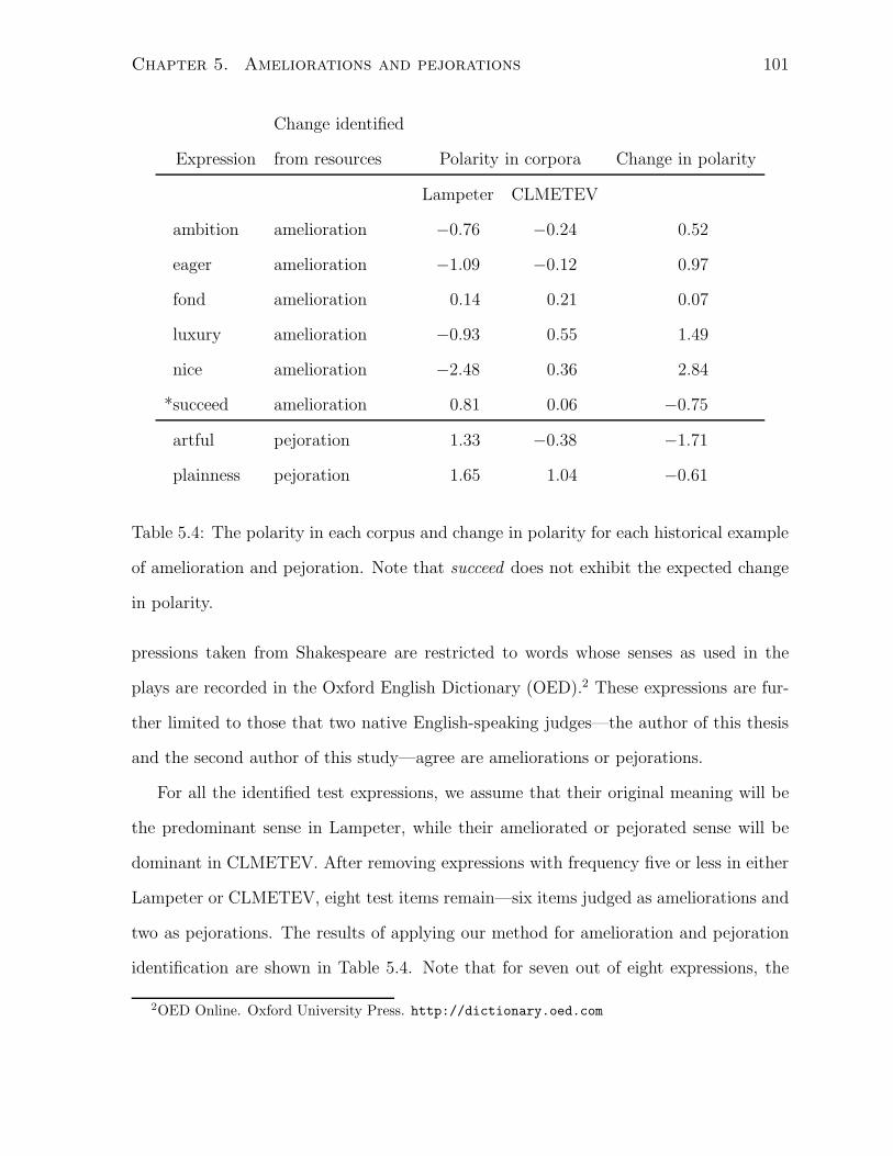
Chapter 5. Ameliorations and pejorations 101
Change identified
Expression from resources Polarity in corpora Change in polarity
Lampeter CLMETEV
ambition amelioration −0.76 −0.24 0.52
eager amelioration −1.09 −0.12 0.97
fond amelioration 0.14 0.21 0.07
luxury amelioration −0.93 0.55 1.49
nice amelioration −2.48 0.36 2.84
*succeed amelioration 0.81 0.06 −0.75
artful pejoration 1.33 −0.38 −1.71
plainness pejoration 1.65 1.04 −0.61
Table 5.4: The polarity in each corpus and change in polarity for each historical example
of amelioration and pejoration. Note that succeed does not exhibit the expected change
in polarity.
pressions taken from Shakespeare are restricted to words whose senses as used in the
plays are recorded in the Oxford English Dictionary (OED).2 These expressions are fur-
ther limited to those that two native English-speaking judges—the author of this thesis
and the second author of this study—agree are ameliorations or pejorations.
For all the identified test expressions, we assume that their original meaning will be
the predominant sense in Lampeter, while their ameliorated or pejorated sense will be
dominant in CLMETEV. After removing expressions with frequency five or less in either
Lampeter or CLMETEV, eight test items remain—six items judged as ameliorations and
two as pejorations. The results of applying our method for amelioration and pejoration
identification are shown in Table 5.4. Note that for seven out of eight expressions, the
2OED Online. Oxford University Press. http://dictionary.oed.com
Chapter 5. Ameliorations and pejorations 102
calculated change in polarity is as expected from the lexical resources; the one exception is
succeed. The calculated polarity is significantly higher for the corpus which is expected to
have higher polarity (CLMETEV in the case of ameliorations, Lampeter for pejorations)
than for the other corpus using a one-tailed paired t-test (p = 0.024).
In this evaluation we used the corpora that we judged to best correspond to the time
periods immediately before and after the predominant sense of the test expressions had
undergone change. Nevertheless, for some of the test expressions, it could be that the
ameliorated or pejorated sense was more common during the time period of the BNC
than that of CLMETEV. However, conducting the same evaluation using the BNC as
opposed to CLMETEV in fact gives very similar results.
5.3.2 Artificial ameliorations and pejorations
We would like to determine whether our method is able to identify known ameliorations
and pejorations; however, as discussed in the previous section, the number of expressions
in our historical dataset thus far is small. We can nevertheless evaluate our method
on artificially created examples of amelioration and pejoration. One possibility for con-
structing such examples is to assume that the usages of words of opposite polarity in two
different corpora are in fact usages of the same word. For example, we could assume that
excellent in Lampeter and poor in CLMETEV are in fact the same word. This would
then be (an artificial example of) a word which has undergone pejoration. If our method
assigns lower polarity to poor in CLMETEV than to excellent in Lampeter, then it has
successfully identified this “pejoration”. This type-based approach to creating artificial
data is inspired by word sense disambiguation evaluations in which the token instances
of two distinct words are used to represent two senses of the same word (e.g., Schutze,
1992).
Selecting appropriate pairs of words to compare in such an evaluation poses numerous
difficulties. For example, it seems that strongly polar words with opposite polarity (e.g.,
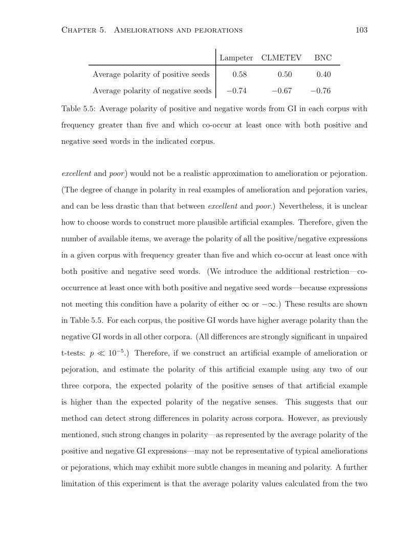
Chapter 5. Ameliorations and pejorations 103
Lampeter CLMETEV BNC
Average polarity of positive seeds 0.58 0.50 0.40
Average polarity of negative seeds −0.74 −0.67 −0.76
Table 5.5: Average polarity of positive and negative words from GI in each corpus with
frequency greater than five and which co-occur at least once with both positive and
negative seed words in the indicated corpus.
excellent and poor) would not be a realistic approximation to amelioration or pejoration.
(The degree of change in polarity in real examples of amelioration and pejoration varies,
and can be less drastic than that between excellent and poor.) Nevertheless, it is unclear
how to choose words to construct more plausible artificial examples. Therefore, given the
number of available items, we average the polarity of all the positive/negative expressions
in a given corpus with frequency greater than five and which co-occur at least once with
both positive and negative seed words. (We introduce the additional restriction—co-
occurrence at least once with both positive and negative seed words—because expressions
not meeting this condition have a polarity of either ∞ or −∞.) These results are shown
in Table 5.5. For each corpus, the positive GI words have higher average polarity than the
negative GI words in all other corpora. (All differences are strongly significant in unpaired
t-tests: p ≪ 10−5.) Therefore, if we construct an artificial example of amelioration or
pejoration, and estimate the polarity of this artificial example using any two of our
three corpora, the expected polarity of the positive senses of that artificial example
is higher than the expected polarity of the negative senses. This suggests that our
method can detect strong differences in polarity across corpora. However, as previously
mentioned, such strong changes in polarity—as represented by the average polarity of the
positive and negative GI expressions—may not be representative of typical ameliorations
or pejorations, which may exhibit more subtle changes in meaning and polarity. A further
limitation of this experiment is that the average polarity values calculated from the two
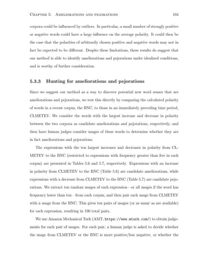
Chapter 5. Ameliorations and pejorations 104
corpora could be influenced by outliers. In particular, a small number of strongly positive
or negative words could have a large influence on the average polarity. It could then be
the case that the polarities of arbitrarily chosen positive and negative words may not in
fact be expected to be different. Despite these limitations, these results do suggest that
our method is able to identify ameliorations and pejorations under idealized conditions,
and is worthy of further consideration.
5.3.3 Hunting for ameliorations and pejorations
Since we suggest our method as a way to discover potential new word senses that are
ameliorations and pejorations, we test this directly by comparing the calculated polarity
of words in a recent corpus, the BNC, to those in an immediately preceding time period,
CLMETEV. We consider the words with the largest increase and decrease in polarity
between the two corpora as candidate ameliorations and pejorations, respectively, and
then have human judges consider usages of these words to determine whether they are
in fact ameliorations and pejorations.
The expressions with the ten largest increases and decreases in polarity from CL-
METEV to the BNC (restricted to expressions with frequency greater than five in each
corpus) are presented in Tables 5.6 and 5.7, respectively. Expressions with an increase
in polarity from CLMETEV to the BNC (Table 5.6) are candidate ameliorations, while
expressions with a decrease from CLMETEV to the BNC (Table 5.7) are candidate pejo-
rations. We extract ten random usages of each expression—or all usages if the word has
frequency lower than ten—from each corpus, and then pair each usage from CLMETEV
with a usage from the BNC. This gives ten pairs of usages (or as many as are available)
for each expression, resulting in 190 total pairs.
We use Amazon Mechanical Turk (AMT, https://www.mturk.com/) to obtain judge-
ments for each pair of usages. For each pair, a human judge is asked to decide whether
the usage from CLMETEV or the BNC is more positive/less negative, or whether the
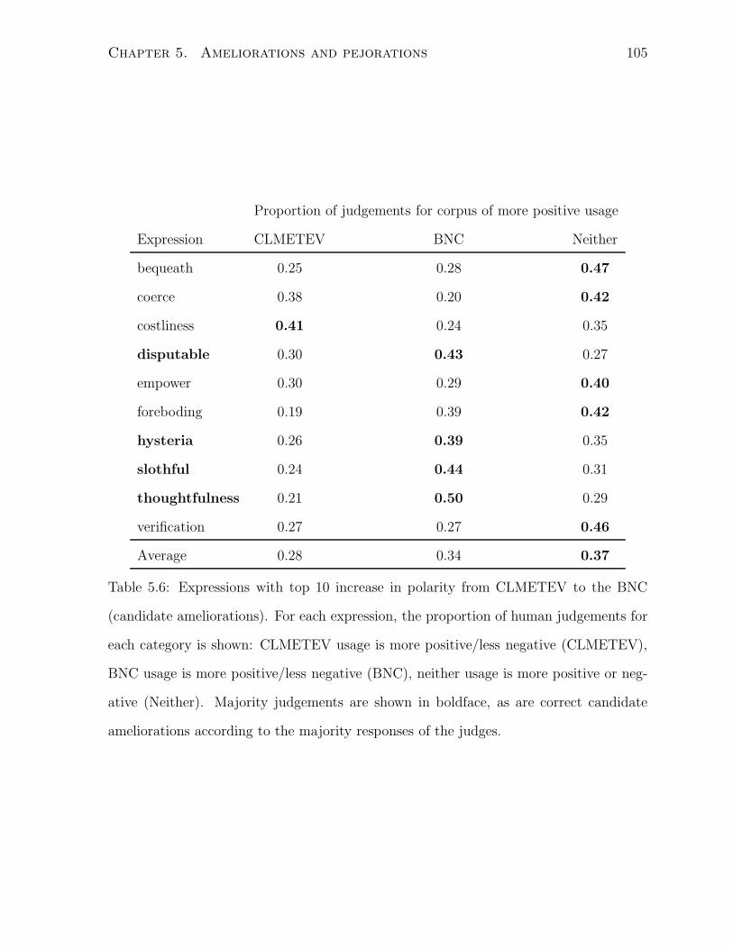
Chapter 5. Ameliorations and pejorations 105
Proportion of judgements for corpus of more positive usage
Expression CLMETEV BNC Neither
bequeath 0.25 0.28 0.47
coerce 0.38 0.20 0.42
costliness 0.41 0.24 0.35
disputable 0.30 0.43 0.27
empower 0.30 0.29 0.40
foreboding 0.19 0.39 0.42
hysteria 0.26 0.39 0.35
slothful 0.24 0.44 0.31
thoughtfulness 0.21 0.50 0.29
verification 0.27 0.27 0.46
Average 0.28 0.34 0.37
Table 5.6: Expressions with top 10 increase in polarity from CLMETEV to the BNC
(candidate ameliorations). For each expression, the proportion of human judgements for
each category is shown: CLMETEV usage is more positive/less negative (CLMETEV),
BNC usage is more positive/less negative (BNC), neither usage is more positive or neg-
ative (Neither). Majority judgements are shown in boldface, as are correct candidate
ameliorations according to the majority responses of the judges.
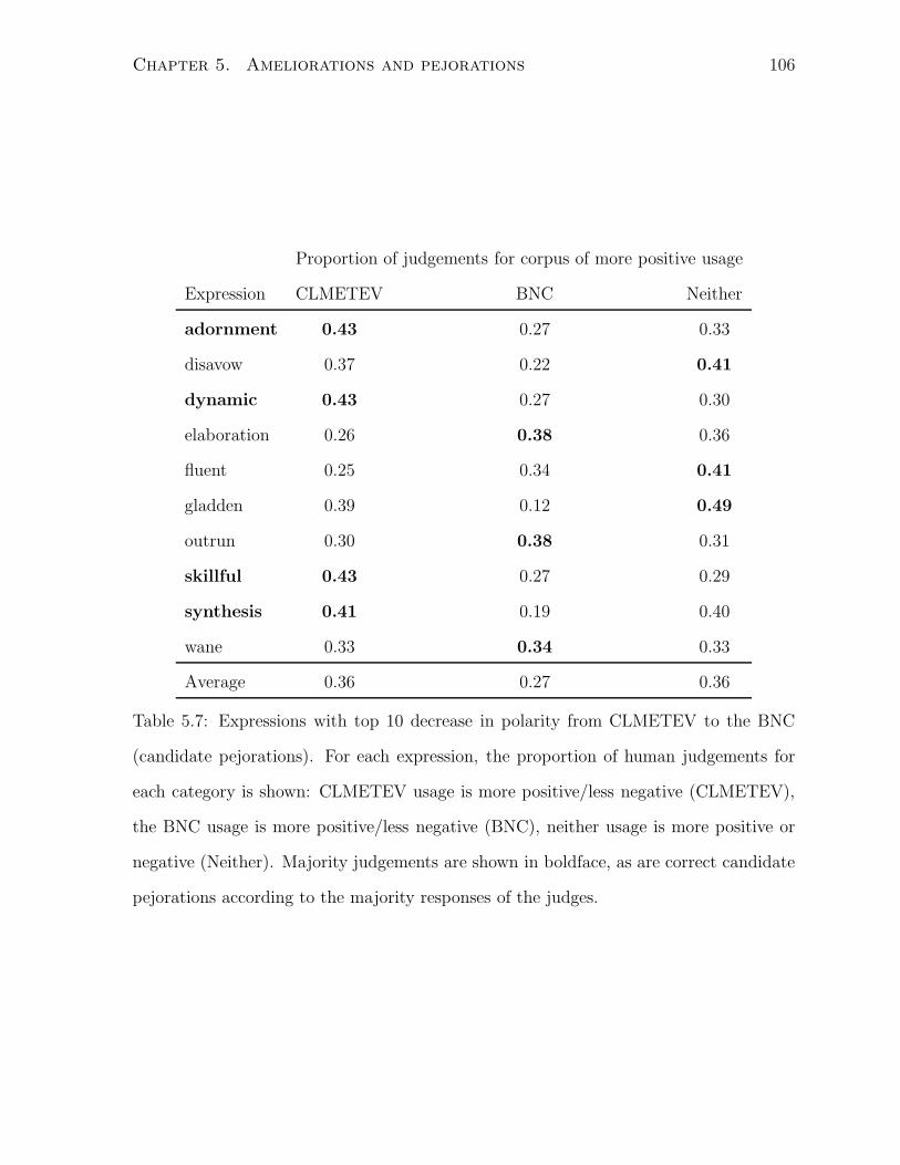
Chapter 5. Ameliorations and pejorations 106
Proportion of judgements for corpus of more positive usage
Expression CLMETEV BNC Neither
adornment 0.43 0.27 0.33
disavow 0.37 0.22 0.41
dynamic 0.43 0.27 0.30
elaboration 0.26 0.38 0.36
fluent 0.25 0.34 0.41
gladden 0.39 0.12 0.49
outrun 0.30 0.38 0.31
skillful 0.43 0.27 0.29
synthesis 0.41 0.19 0.40
wane 0.33 0.34 0.33
Average 0.36 0.27 0.36
Table 5.7: Expressions with top 10 decrease in polarity from CLMETEV to the BNC
(candidate pejorations). For each expression, the proportion of human judgements for
each category is shown: CLMETEV usage is more positive/less negative (CLMETEV),
the BNC usage is more positive/less negative (BNC), neither usage is more positive or
negative (Neither). Majority judgements are shown in boldface, as are correct candidate
pejorations according to the majority responses of the judges.
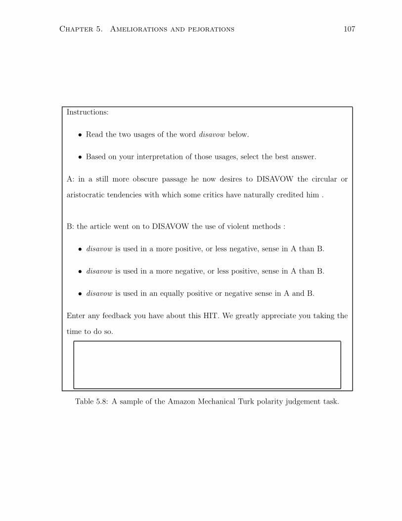
Chapter 5. Ameliorations and pejorations 107
Instructions:
• Read the two usages of the word disavow below.
• Based on your interpretation of those usages, select the best answer.
A: in a still more obscure passage he now desires to DISAVOW the circular or
aristocratic tendencies with which some critics have naturally credited him .
B: the article went on to DISAVOW the use of violent methods :
• disavow is used in a more positive, or less negative, sense in A than B.
• disavow is used in a more negative, or less positive, sense in A than B.
• disavow is used in an equally positive or negative sense in A and B.
Enter any feedback you have about this HIT. We greatly appreciate you taking the
time to do so.
Table 5.8: A sample of the Amazon Mechanical Turk polarity judgement task.
Chapter 5. Ameliorations and pejorations 108
two usages are equally positive/negative. A sample of this AMT polarity judgement task
is presented in Table 5.8. We solicit responses from ten judges for each pair of usages,
and pay $0.05 per judgement.
The judgements obtained from AMT are shown in Tables 5.6 and 5.7. For each
candidate amelioration or pejoration the proportion of responses that the usage from
CLMETEV, the BNC, or neither is more positive/less negative is shown. For each ex-
pression, the majority response is indicated in boldface. In the case of both candidate
ameliorations and pejorations, four out of ten items are correct according to the AMT
judgements; these expressions are also shown in boldface. Taking the AMT judgements
as a gold-standard, this corresponds to a precision of 40%. (We cannot calculate recall
because this would require manually identifying all of the ameliorations and pejorations
between the two corpora.) We also consider the average proportion of responses for
each category (CLMETEV usage is more positive/less negative, BNC usage is more
positive/less negative, neither usage is more positive or negative) for the candidate ame-
liorations and pejorations (shown in the last row of Tables 5.6 and 5.7, respectively).
Here we note that for candidate ameliorations the average proportion of responses that
the BNC usage is more positive is higher than the average proportion of responses that
the CLMETEV usage is more positive, and vice versa for candidate pejorations. This
is an encouraging result, but in one-tailed paired t-tests it is not found to be significant
for candidate ameliorations (p = 0.12), although it is marginally significant for candidate
pejorations (p = 0.05).
We also consider an evaluation methodology in which we ignore the judgements for
usage pairs for which the judgements are roughly uniformly distributed across the three
categories. For each usage pair, if the proportion of judgements of the most frequent
judgement is greater than 0.5 then this pair is assigned the category of the most frequent
judgement, otherwise we ignore the judgements for this pair. We then count these re-
sulting judgements for each candidate amelioration and pejoration. In this alternative
Chapter 5. Ameliorations and pejorations 109
evaluation, the overall results are quite similar to those presented in Tables 5.6 and 5.7.
These results are not very strong from the perspective of a fully-automated system
for identifying ameliorations and pejorations; in the case of both candidate ameliorations
and pejorations only four of the ten items are judged as correct by humans. Nevertheless,
these results do indicate that this approach could be useful as a semi-automated tool to
help in the identification of new senses, particularly since the methods are inexpensive
to apply.
5.4 Amelioration or pejoration of the seeds
Our method for identifying ameliorations and pejorations relies on knowing the polarity of
a large number of seed words. However, a seed word itself may also undergo amelioration
or pejoration, and therefore its polarity may in fact differ from what we assume it to
be in the seed sets to produce a noisy set of seed words. Here we explore the extent
to which noisy seed words—i.e., seed words labelled with incorrect polarity—affect the
performance of our method. We begin by randomly selecting n% of the positive seed
words, and n% of the negative seed words, and swapping these items in the seed sets. We
then conduct a leave-one-out experiment, using the same methodology as in Section 5.2,
in which we use the noisy seed words to calculate the polarity of all items in the GI lexicon
which co-occur at least five times with seed words in the corpus under consideration.
We consider each n in {5, 10, 15, 20}, and repeat each experiment five times, randomly
selecting the seed words whose polarity is changed in each trial. The average accuracy
over the five trials is shown in Figure 5.1.
We observe a similar trend for all three corpora: the average accuracy decreases as the
percentage of noisy seed words increases. However, with a small amount of noise in the
seed sets, 5%, the reduction in absolute average accuracy is small, only 1–2 percentage
points, for each corpus. Furthermore, when the percentage of noisy seed words is in-
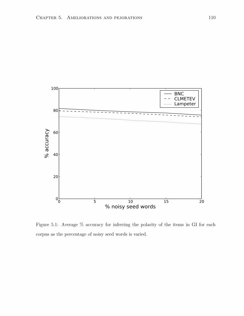
Chapter 5. Ameliorations and pejorations 110
0 5 10 15 20% noisy seed words
0
20
40
60
80
100
% a
ccura
cy
BNCCLMETEVLampeter
Figure 5.1: Average % accuracy for inferring the polarity of the items in GI for each
corpus as the percentage of noisy seed words is varied.
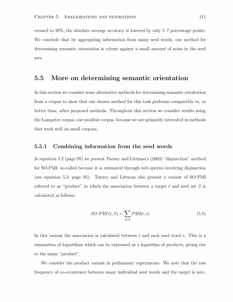
Chapter 5. Ameliorations and pejorations 111
creased to 20%, the absolute average accuracy is lowered by only 5–7 percentage points.
We conclude that by aggregating information from many seed words, our method for
determining semantic orientation is robust against a small amount of noise in the seed
sets.
5.5 More on determining semantic orientation
In this section we consider some alternative methods for determining semantic orientation
from a corpus to show that our chosen method for this task performs comparably to, or
better than, other proposed methods. Throughout this section we consider results using
the Lampeter corpus, our smallest corpus, because we are primarily interested in methods
that work well on small corpora.
5.5.1 Combining information from the seed words
In equation 5.2 (page 95) we present Turney and Littman’s (2003) “disjunction” method
for SO-PMI, so-called because it is estimated through web queries involving disjunction
(see equation 5.3, page 95). Turney and Littman also present a variant of SO-PMI
referred to as “product” in which the association between a target t and seed set S is
calculated as follows:
SO-PMI (t, S) =∑
s∈S
PMI(t, s) (5.5)
In this variant the association is calculated between t and each seed word s. This is a
summation of logarithms which can be expressed as a logarithm of products, giving rise
to the name “product”.
We consider the product variant in preliminary experiments. We note that the raw
frequency of co-occurrence between many individual seed words and the target is zero.
Chapter 5. Ameliorations and pejorations 112
Following Turney and Littman we smooth frequencies using Laplace smoothing. We
consider a range of smoothing factors, but find this method to perform poorly in all
cases. The smoothed zero frequencies appear to have a very large effect on the calculated
polarities. We believe this to be the reason for the poor performance of this method.
The disjunction variant that we adopt for our method counts co-occurrence between the
target and any positive/negative seed word. It is unlikely that the target would have
a frequency of co-occurrence of zero with all the positive or negative seed words, and
therefore the method of smoothing used has less impact on the calculated polarities.
(Indeed, for our experiments it was not necessary to smooth the frequencies.) We believe
this is why the disjunction variant performs better in our experiments.
It is also worth noting that Turney and Littman find the product and disjunction
variants to perform similarly on their smallest corpus (which at approximately ten mil-
lion words is much larger than our smallest corpus, Lampeter). The disjunction variant
is more efficient to calculate than the product variant in Turney and Littman’s experi-
mental setup because it requires issuing less search engine queries. Turney and Littman
therefore argue that for small corpora disjunction is more appropriate. However, in our
experimental setup the two approaches require equal computational cost, so this reason
for choosing the disjunction variant does not apply.
5.5.2 Number of seed words
In our method for inferring semantic orientation we assume that it is necessary to use
a large number of seed words to compensate for the relatively small size of our corpora.
Here we support this assumption by considering the results of using a smaller number of
seed words.
We compare the accuracy for inferring the polarity of items in GI using the fourteen
seed words from Turney and Littman (2003) with the accuracy using the words from GI
as seed words (3610 seeds). Because of our frequency restriction that items must occur
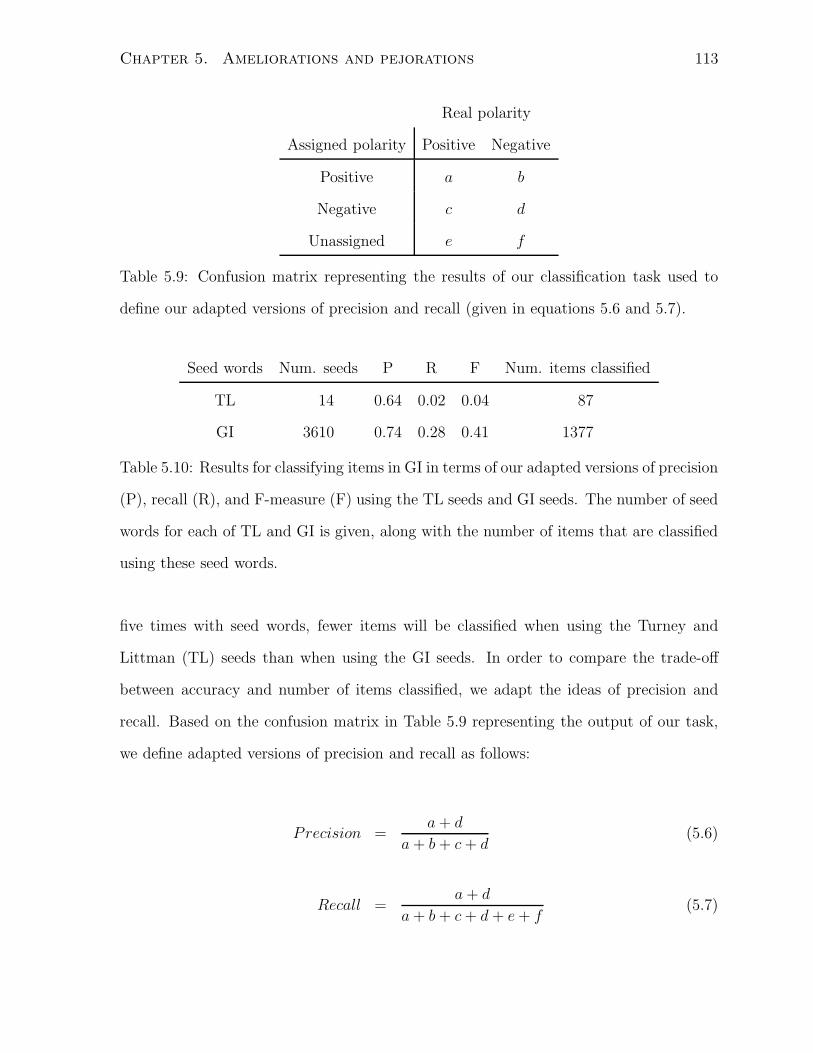
Chapter 5. Ameliorations and pejorations 113
Real polarity
Assigned polarity Positive Negative
Positive a b
Negative c d
Unassigned e f
Table 5.9: Confusion matrix representing the results of our classification task used to
define our adapted versions of precision and recall (given in equations 5.6 and 5.7).
Seed words Num. seeds P R F Num. items classified
TL 14 0.64 0.02 0.04 87
GI 3610 0.74 0.28 0.41 1377
Table 5.10: Results for classifying items in GI in terms of our adapted versions of precision
(P), recall (R), and F-measure (F) using the TL seeds and GI seeds. The number of seed
words for each of TL and GI is given, along with the number of items that are classified
using these seed words.
five times with seed words, fewer items will be classified when using the Turney and
Littman (TL) seeds than when using the GI seeds. In order to compare the trade-off
between accuracy and number of items classified, we adapt the ideas of precision and
recall. Based on the confusion matrix in Table 5.9 representing the output of our task,
we define adapted versions of precision and recall as follows:
Precision =a + d
a + b + c + d(5.6)
Recall =a + d
a + b + c + d + e + f(5.7)
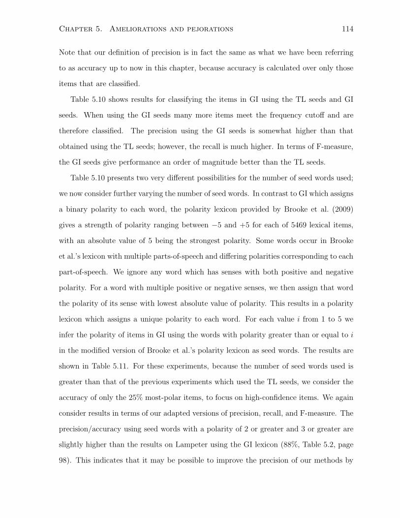
Chapter 5. Ameliorations and pejorations 114
Note that our definition of precision is in fact the same as what we have been referring
to as accuracy up to now in this chapter, because accuracy is calculated over only those
items that are classified.
Table 5.10 shows results for classifying the items in GI using the TL seeds and GI
seeds. When using the GI seeds many more items meet the frequency cutoff and are
therefore classified. The precision using the GI seeds is somewhat higher than that
obtained using the TL seeds; however, the recall is much higher. In terms of F-measure,
the GI seeds give performance an order of magnitude better than the TL seeds.
Table 5.10 presents two very different possibilities for the number of seed words used;
we now consider further varying the number of seed words. In contrast to GI which assigns
a binary polarity to each word, the polarity lexicon provided by Brooke et al. (2009)
gives a strength of polarity ranging between −5 and +5 for each of 5469 lexical items,
with an absolute value of 5 being the strongest polarity. Some words occur in Brooke
et al.’s lexicon with multiple parts-of-speech and differing polarities corresponding to each
part-of-speech. We ignore any word which has senses with both positive and negative
polarity. For a word with multiple positive or negative senses, we then assign that word
the polarity of its sense with lowest absolute value of polarity. This results in a polarity
lexicon which assigns a unique polarity to each word. For each value i from 1 to 5 we
infer the polarity of items in GI using the words with polarity greater than or equal to i
in the modified version of Brooke et al.’s polarity lexicon as seed words. The results are
shown in Table 5.11. For these experiments, because the number of seed words used is
greater than that of the previous experiments which used the TL seeds, we consider the
accuracy of only the 25% most-polar items, to focus on high-confidence items. We again
consider results in terms of our adapted versions of precision, recall, and F-measure. The
precision/accuracy using seed words with a polarity of 2 or greater and 3 or greater are
slightly higher than the results on Lampeter using the GI lexicon (88%, Table 5.2, page
98). This indicates that it may be possible to improve the precision of our methods by
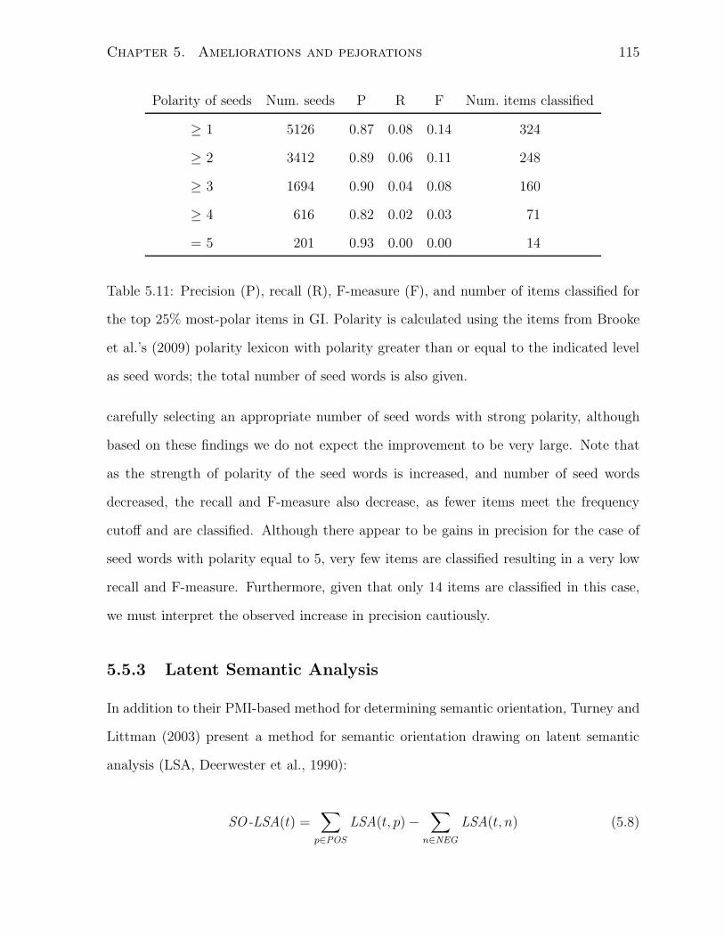
Chapter 5. Ameliorations and pejorations 115
Polarity of seeds Num. seeds P R F Num. items classified
≥ 1 5126 0.87 0.08 0.14 324
≥ 2 3412 0.89 0.06 0.11 248
≥ 3 1694 0.90 0.04 0.08 160
≥ 4 616 0.82 0.02 0.03 71
= 5 201 0.93 0.00 0.00 14
Table 5.11: Precision (P), recall (R), F-measure (F), and number of items classified for
the top 25% most-polar items in GI. Polarity is calculated using the items from Brooke
et al.’s (2009) polarity lexicon with polarity greater than or equal to the indicated level
as seed words; the total number of seed words is also given.
carefully selecting an appropriate number of seed words with strong polarity, although
based on these findings we do not expect the improvement to be very large. Note that
as the strength of polarity of the seed words is increased, and number of seed words
decreased, the recall and F-measure also decrease, as fewer items meet the frequency
cutoff and are classified. Although there appear to be gains in precision for the case of
seed words with polarity equal to 5, very few items are classified resulting in a very low
recall and F-measure. Furthermore, given that only 14 items are classified in this case,
we must interpret the observed increase in precision cautiously.
5.5.3 Latent Semantic Analysis
In addition to their PMI-based method for determining semantic orientation, Turney and
Littman (2003) present a method for semantic orientation drawing on latent semantic
analysis (LSA, Deerwester et al., 1990):
SO-LSA(t) =∑
p∈POS
LSA(t, p) −∑
n∈NEG
LSA(t, n) (5.8)

Chapter 5. Ameliorations and pejorations 116
According to SO-LSA the semantic orientation of a word is the difference between its
similarity (using LSA) with known positive and negative seed words. The key difference
between SO-LSA and SO-PMI is that SO-LSA assumes that words with similar polarity
will tend to occur in similar contexts while SO-PMI assumes that words with similar
polarity will tend to co-occur.
Turney and Littman’s findings suggest that for small corpora, SO-LSA may be more
appropriate than SO-PMI. This approach therefore seems promising given our interest in
small corpora. Turney and Littman use an equal number of positive and negative seeds,
whereas in our study the size of the seed sets differ. We account for this by dividing the
association with the positive and negative seeds by the size of the positive and negative
seed sets, respectively, as below:
SO-LSA(t) =
∑
p∈POS LSA(t, p)
|POS |−
∑
n∈NEG LSA(t, n)
|NEG |(5.9)
The Lampeter corpus consists of 122 documents averaging approximately 9000 words
each. It is unlikely that such a large context will be useful for capturing information
related to polarity. Therefore, whereas Turney and Littman construct a term–document
matrix, we construct a term–sentence matrix. (The documents used by Turney and
Littman are rather short, with an average length of approximately 260 words.) In these
experiments we use the words from GI as seeds, and restrict our evaluation to words with
frequency greater than 5 in Lampeter. We consider a range of values of k (the dimen-
sionality of the resulting term vectors); however, in no case are the results substantially
above the baseline. It may be the case that in our experimental setup the term–sentence
matrix is too sparse to effectively capture polarity. In the future we intend to consider
a term–paragraph matrix to address this. (We have not yet done this experiment as we
found some inconsistencies in the paragraph mark-up of Lampeter which we must resolve
Chapter 5. Ameliorations and pejorations 117
before doing so.)
5.6 Summary of contributions
This is the first computational study of amelioration and pejoration. We adapt an estab-
lished corpus-based method for identifying polarity for use on small corpora, and show
that it performs reasonably well. We then apply this method for determining polarity to
corpora of texts from differing time periods to identify ameliorations and pejorations. In
evaluations on a small dataset of historical ameliorations and pejorations, and artificial
examples of amelioration and pejoration, we show that our proposed method successfully
captures diachronic differences in polarity. We also apply this method to find words
which have undergone amelioration and pejoration in corpora. The results of this exper-
iment indicate that although our proposed method does not perform well on the task of
fully-automatic identification of new senses, it may be useful as a semi-automated tool
for finding new word senses.
Chapter 6
Conclusions
This chapter summarizes the contributions this thesis has made and then describes a
number of directions for future work.
6.1 Summary of contributions
The hypothesis of this thesis is that knowledge about word formation processes and
types of semantic change can improve the automatic acquisition of aspects of the syntax
and semantics of neologisms. Evidence supporting this hypothesis has been found in
the studies of lexical blends, text messaging forms, and ameliorations and pejorations
presented in this thesis. In the study of lexical blends in Chapter 3, knowledge of the
ways in which blends are formed and how people interpret them is exploited in a method
for automatically inferring the source words of novel blends, an important step in the
inference of the syntax and semantics of a blend. Moreover, the same information is used
to distinguish blends from other types of neologisms. In Chapter 4, the common ways
in which text messaging forms are created from their standard forms is exploited for
the task of text message normalization. By considering word formation types in texting
language, we are able to develop an unsupervised model for text message normalization
that performs as well as a supervised approach. In Chapter 5 we consider the use of
118
Chapter 6. Conclusions 119
knowledge of types of semantic change to identify new word senses. Specifically, by
drawing on knowledge of amelioration and pejoration—two types of semantic change—
we are able to identify words that have undergone these processes.
Computational work to date on lexical acquisition has concentrated on the context
in which an unknown word occurs to infer aspects of its lexical entry; typically such
approaches exploit statistical distributional information or expensive manually-crafted
lexical resources (see discussion in Chapter 2). However, in the case of neologisms, nei-
ther of these sources of information is necessarily available. New words are expected
to be low frequency due to the recency of their coinage, and therefore distributional
information is not reliable in this case. Approaches to lexical acquisition that rely heav-
ily on lexical resources are typically limited to a particular domain; new words occur
throughout a language, and therefore such approaches are not generally applicable to
neologisms. This thesis finds evidence to support the hypothesis that knowledge of word
formation processes and types of semantic change can be exploited for lexical acquisition
of neologisms, where these other knowledge sources cannot be relied upon. This thesis
sets the stage for further research into lexical acquisition that considers word formation
processes and types of semantic change and what can be inferred from this information.
Moreover, since these methods are particularly well-suited to new words, this thesis will
encourage further research on neologisms, which have not been extensively considered in
computational linguistics.
Chapter 3 presents the first computational study of lexical blends. This frequent
new word type had been previously ignored in computational linguistics. We present
a statistical method for inferring the source words of a blend—an important first step
in the semantic interpretation of a blend—that draws on linguistic observations about
blends and cognitive factors that may play a role in their interpretation. The proposed
method achieves an accuracy of 40% on a test set of 324 novel unseen blends. We also
present preliminary methods for identifying an unknown word as a blend.
Chapter 6. Conclusions 120
In our study of blends we find strikingly different results when our methods are
applied to newly-coined blends versus established blends found in a dictionary. This
finding emphasizes the importance of testing methods for processing neologisms on truly
new expressions. We annotate a set of 1,186 recently-coined expressions (including the
324 blends used in evaluation discussed above) for their word formation type, which will
support future research on neologisms.
We describe the first unsupervised approach to text messaging normalization in Chap-
ter 4; normalization is an important step that must be taken before other NLP tasks, such
as machine translation, can be done. By considering common word formation processes
in text messaging, we are able to develop an unsupervised method which gives perfor-
mance on par with that of a supervised system on the same dataset. Moreover, since our
approach is unsupervised, it can be adapted to other media without the cost of devel-
oping a manually-annotated training resource. This is particularly important given that
non-standard forms similar to those found in text messaging are common in other popular
forms of computer-mediated communication, such as Twitter (http://twitter.com).
Chapter 5 describes the first computational work focusing on the processes of ame-
lioration and pejoration. In this work we adapt an established corpus-based method for
inferring polarity to the task of identifying ameliorations and pejorations. We propose
an unsupervised method for this task and show that our proposed method is able to
successfully identify historical ameliorations and pejorations, as well as artificial exam-
ples of amelioration and pejoration. We also apply this method to find words which
have undergone amelioration and pejoration in recent corpora. In addition to being the
first computational work on amelioration and pejoration, this study is one of only a
small number of computational studies of diachronic semantic change, an exciting new
interdisciplinary research direction.
Chapter 6. Conclusions 121
6.2 Future directions
In this section we discuss a number of future directions related to each of the three studies
presented in Chapters 3–5.
6.2.1 Lexical blends
There are a number of ways in which the model for source word identification presented
in Section 3.1 could potentially be improved. The present results using the modified
perceptron algorithm are not an improvement over the rather unsophisticated feature
ranking approach. As discussed in Section 3.4.2.3, machine learning methods that do not
assume that the training data is linearly separable, such as that described by Joachims
(2002), may give an improvement over our current methods.
The features used in the proposed model do not take into account the context in which
a given blend occurs. However, blends often occur with their source words nearby in a
text, although unlike acronyms (discussed in Section 2.1.3.1) there do not appear to be as
clear textual indicators of the relationship between the words (e.g., a longform followed
by its acronym in parentheses). Nevertheless, the words that occur in a window of words
around a blend may be very informative as to the blend’s source words. A simple feature
capturing whether a candidate source word is used within a window of words around a
usage of a blend may be a very powerful feature. Note that such contextual information
could be exploited even if just one instance of a given blend is observed.
Contextual information could also be used to improve our approach to blend identi-
fication (see Section 3.5). If an unknown word is used with two of its candidate source
words occurring nearby in the text, and those candidate source words are likely source
words according to the model presented in Section 3.1, the unknown word may be likely
to be a blend.
In Chapter 3 we focus on source word identification because it is an important first
Chapter 6. Conclusions 122
step in the semantic interpretation of blends. However, once a blend’s source words have
been identified, their semantic relationship must be determined in order to interpret the
expression. Classifying blends as one of a pre-determined number of semantic relationship
types is one way to approach this task.
Algeo (1977) gives a categorization of blends which consists of two broad categories:
syntagmatic blends, such as webinar (web seminar), can be viewed as a contraction of
two words that occur consecutively in text; associative blends, on the other hand, involve
source words that are related in some way. For example, brunch combines breakfast and
lunch which are both types of meal, whereas a chocoholic is addicted to chocolate similarly
to the way an alcoholic is addicted to alcohol.
A classification of blend semantics based on the ontological relationship between a
blend and its source words may be particularly useful for computational blend inter-
pretation. Many syntagmatic blends are hyponyms of their second source word (e.g.,
webinar is a type of seminar). Some associative blends are a hyponym of the lowest
common subsumer of their source words (e.g., breakfast and lunch are both hyponyms
of meal, as is brunch). However, the ontological relationship between chocolate, alco-
holic, and chocoholic is less clear. Moreover, blends such as momic—a mom who is a
(stand up) comic—appear to be hyponyms of both their source words. These expressions
demonstrate that there are clearly many challenges involved in developing a classification
scheme for blends appropriate for their semantic interpretation; this remains a topic for
future work.
6.2.2 Text messaging forms
The model for text message normalization presented in Chapter 4 uses a unigram lan-
guage model. One potential way to improve the accuracy of this system is through the
use of a higher-order n-gram language model. However, Choudhury et al.’s (2007) study
of text message normalization finds that a bigram language model does not outperform
Chapter 6. Conclusions 123
a unigram language model. On the other hand Choudhury et al. estimate their language
model from a balanced corpus of English (the British National Corpus, Burnard, 2007);
estimating this language model from a medium that is more similar to that of text mes-
saging, such as the World Wide Web, may result in higher-order n-gram language models
that do outperform a unigram language model for this task.
We consider unsupervised approaches to text message normalization because we ob-
serve that similar abbreviated forms are common in other types of computer-mediated
communication, and want a model which can be easily adapted to such media without
the cost of developing a large manually-annotated resource. Twitter is a microblogging
service which has become very popular recently. Tweets—the messages a user posts
on Twitter—are limited to 140 characters. Perhaps due to this limited space, and also
possibly due to the desire to communicate in an informal register, tweets exhibit many
shortened and non-standard forms similar to text messages. Because Twitter has be-
come so popular, there are many interesting opportunities to apply NLP technology to
this medium. For example, Twitter can be used to determine public opinion on some
product, or find trends in popular topics. However, in order to effectively apply methods
for such NLP tasks, the text must first be normalized. Adapting our proposed method
for text message normalization to Twitter is therefore a direction for future work that
could directly benefit the many applications processing tweets.
6.2.3 Ameliorations and pejorations
There are a number of ways to potentially improve the method for estimating polarity
used in Chapter 5. We intend to consider incorporating syntactic information, such as
the target expression’s part-of-speech, as well as linguistic knowledge about common
patterns that indicate polarity; for example, adjectives co-ordinated by but often have
opposite semantic orientation. Furthermore, although our experiments so far using LSA
to estimate polarity have not found this method to perform better than PMI-based
Chapter 6. Conclusions 124
methods, we intend to further consider LSA. In particular, we intend to re-examine the
context used when constructing the co-occurrence matrix (i.e., sentence, paragraph, or
document).
The corpora used in this study, although all consisting of British English, are not com-
parable, i.e., they were not constructed using the same or similar sampling strategies. It
is possible that any differences in polarity found between these corpora can be attributed
to differences in the composition of the corpora. In future work, we intend to evaluate
our methods on more comparable corpora; for example, the Brown Corpus (Kucera and
Francis, 1967) and Frown Corpus (Hundt et al., 1999)—comparable corpora of American
English from the 1960s and 1990s, respectively—could be used to study changes in polar-
ity between these time periods in American English. We are also excited about applying
our methods to very recent corpora to identify new word senses.
In the present study we have considered amelioration and pejoration only across time.
However, words may have senses of differing polarity which are specific to a particular
speech community. In the future, we intend to apply our methods to comparable corpora
of the same language, but different geographical regions, such as the International Corpus
of English (http://ice-corpora.net/ice/) to identify words with differing semantic
orientation in these varieties of English.
We also intend to consider ways to improve the evaluation of our methods for identi-
fying ameliorations and pejorations. We are working to enlarge our dataset of expressions
known to have undergone amelioration or pejoration in order to conduct a larger-scale
evaluation on historical examples of these processes. We further intend to conduct a
more wide-scale human evaluation of our experiments on hunting for ameliorations and
pejorations. In particular, in our current evaluation, each usage participates in only one
pairing; the exact pairings chosen therefore heavily influence the outcome. In the future
we will include each usage in multiple pairings in order to reduce this effect.
Chapter 6. Conclusions 125
6.2.4 Corpus-based studies of semantic change
The meaning of a word can vary with respect to a variety of sociolinguistic variables,
such as time period, geographical location, sex, age, and socio-economic status. As
noted in Section 2.3, identifying new word senses is a major challenge for lexicography;
identifying unique regional word senses poses similar challenges. Automatic methods for
identifying words that vary in meaning along one of the aforementioned variables would
be very beneficial for lexicography focusing on specific speech communities (defined by
these variables), and also the study of language variation.
The study on automatically identifying ameliorations and pejorations presented in
Chapter 5 is a specific instance of this research problem. One of my longterm research
goals is accurate methods for detecting semantic change—including ameliorations and
pejorations, but also more general processes such as widening and narrowing—across
any sociolinguistic variable.
Bibliography
Steven Abney. 1991. Parsing by chunks. In Robert Berwick, Steven Abney, and Carol
Tenny, editors, Principle-Based Parsing: Computation and Psycholinguistics, pages
257–278. Kluwer Academic Publishers, Dordrecht, The Netherlands.
Beatrice Alex. 2006. Integrating language knowledge resources to extend the English
inclusion classifier to a new language. In Proceedings of the Fifth International Con-
ference on Language Resources and Evaluation (LREC 2006), pages 2431–2436. Genoa,
Italy.
Beatrice Alex. 2008. Comparing corpus-based to web-based lookup techniques for auto-
matic English inclusion detection. In Proceedings of the Sixth International Conference
on Language Resources and Evaluation (LREC 2008), pages 2693–2697. Marrakech,
Morocco.
John Algeo. 1977. Blends, a structural and systemic view. American Speech, 52(1/2):47–
64.
John Algeo. 1980. Where do all the new words come from. American Speech, 55(4):264–
277.
John Algeo, editor. 1991. Fifty Years Among the New Words. Cambridge University
Press, Cambridge.
126
BIBLIOGRAPHY 127
John Algeo. 1993. Desuetude among new words. International Journal of Lexicography,
6(4):281–293.
Keith Allan and Kate Burridge. 1991. Euphemism & Dysphemism: Language Used as
Shield and Weapon. Oxford University Press, New York.
Stephen R. Anderson. 1992. A-Morphous Morphology. Cambridge University Press,
Cambridge.
B. T. Sue Atkins and Michael Rundell. 2008. The Oxford Guide to Practical Lexicography.
Oxford University Press, Oxford.
AiTi Aw, Min Zhang, Juan Xiao, and Jian Su. 2006. A phrase-based statistical model for
SMS text normalization. In Proceedings of the COLING/ACL 2006 Main Conference
Poster Sessions, pages 33–40. Sydney, Australia.
John Ayto, editor. 1990. The Longman Register of New Words, volume 2. Longman,
London.
John Ayto. 2006. Movers and Shakers: A Chronology of Words that Shaped our Age.
Oxford University Press, Oxford.
R. Harald Baayen, Richard Piepenbrock, and Leon Gulikers. 1995. The CELEX Lexical
Database (Release 2). Linguistic Data Consortium, Philadelphia.
R. Harald Baayen and Antoinette Renouf. 1996. Chronicling the Times: Productive
lexical innovations in an English newspaper. Language, 72(1):69–96.
Kirk Baker and Chris Brew. 2008. Statistical identification of English loanwords in
Korean using automatically generated training data. In Proceedings of the Sixth In-
ternational Conference on Language Resources and Evaluation (LREC 2008), pages
1159–1163. Marrakech, Morocco.
BIBLIOGRAPHY 128
Timothy Baldwin and Aline Villavicencio. 2002. Extracting the unextractable: A case
study on verb-particles. In Proceedings of the Sixth Conference on Computational
Natural Language Learning (CoNLL-2002), pages 98–104. Taipei, Taiwan.
Clarence L. Barnhart. 1978. American lexicography, 1945–1973. American Speech,
53(2):83–140.
Clarence L. Barnhart, Sol Steinmetz, and Robert K. Barnhart. 1973. The Barnhart
Dictionary of New English Since 1963. Barnhart/Harper & Row, Bronxville, NY.
David K. Barnhart. 1985. Prizes and pitfalls of computerized searching for new words
for dictionaries. Dictionaries, 7:253–260.
David K. Barnhart. 2007. A calculus for new words. Dictionaries, 28:132–138.
Susan Bartlett, Grzegorz Kondrak, and Colin Cherry. 2008. Automatic syllabification
with structured SVMs for letter-to-phoneme conversion. In Proceedings of the 46th
Annual Meeting of the Association for Computational Linguistics (ACL-08): Human
Language Technologies, pages 568–576. Columbus, Ohio.
Laurie Bauer. 1983. English Word-formation. Cambridge University Press, Cambridge.
Beata Beigman Klebanov, Eyal Beigman, and Daniel Diermeier. 2009. Discourse topics
and metaphors. In Proceedings of the NAACL HLT 2009 Workshop on Computational
Approaches to Linguistic Creativity (CALC-2009), pages 1–8. Boulder, CO.
David M. Blei, Andrew Y. Ng, and Michael I. Jordan. 2003. Latent dirichlet allocation.
Journal of Machine Learning Research, 3:993–1022.
Valerie M. Boulanger. 1997. What Makes a Coinage Successful?: The Factors Influencing
the Adoption of English New Words. Ph.D. thesis, University of Georgia.
Thorsten Brants and Alex Franz. 2006. Web 1T 5-gram Corpus version 1.1.
BIBLIOGRAPHY 129
Eric Brill. 1994. Some advances in transformation-based part of speech tagging. In
Proceedings of the Twelfth National Conference on Artificial Intelligence, pages 722–
727. Seattle, Washington.
Eric Brill and Robert C. Moore. 2000. An improved error model for noisy channel
spelling correction. In Proceedings of the 38th Annual Meeting of the Association for
Computational Linguistics, pages 286–293. Hong Kong.
Laurel Brinton and Leslie Arnovick, editors. 2005. The English Language: A Linguistic
History. Oxford University Press.
Julian Brooke, Milan Tofilosky, and Maite Taboada. 2009. Cross-linguistic sentiment
analysis: From English to Spanish. In Proceedings of Recent Advances in Natural
Language Processing (RANLP-2009). Borovets, Bulgaria.
Ian Brookes. 2007. New words and corpus frequency. Dictionaries, 28:142–145.
Lou Burnard. 2007. Reference guide for the British National Corpus (XML Edition).
Oxford University Computing Services.
Lyle Campbell. 2004. Historical Linguistics: An Introduction. MIT Press, Cambridge,
MA.
Claire Cardie. 1993. A case-based approach to knowledge acquisition for domain-specific
sentence analysis. In Proceedings of the Eleventh National Conference on Artificial
Intelligence, pages 798–803. Washington, DC.
Yejin Choi and Claire Cardie. 2009. Adapting a polarity lexicon using integer linear
programming for domain-specific sentiment classification. In Proceedings of the 2009
Conference on Empirical Methods in Natural Language Processing (EMNLP-2009),
pages 590–598. Singapore.
BIBLIOGRAPHY 130
Monojit Choudhury, Rahul Saraf, Vijit Jain, Animesh Mukherjee, Sudeshna Sarkar, and
Anupam Basu. 2007. Investigation and modeling of the structure of texting language.
International Journal of Document Analysis and Recognition, 10(3/4):157–174.
Kenneth W. Church and Patrick Hanks. 1990. Word association norms, mutual informa-
tion, and lexicography. Computational Linguistics, 16(1):22–29.
Michael Collins. 2003. Head-driven statistical models for natural language parsing. Com-
putational Linguistics, 29(4):589–637.
Paul Cook and Suzanne Stevenson. 2007. Automagically inferring the source words of
lexical blends. In Proceedings of the Tenth Conference of the Pacific Association for
Computational Linguistics (PACLING-2007), pages 289–297. Melbourne, Australia.
Paul Cook and Suzanne Stevenson. 2009. An unsupervised model for text message nor-
malization. In Proceedings of the NAACL HLT 2009 Workshop on Computational
Approaches to Linguistic Creativity (CALC-2009), pages 71–78. Boulder, CO.
Paul Cook and Suzanne Stevenson. 2010a. Automatically identifying changes in the
semantic orientation of words. In Proceedings of the Seventh International Conference
on Language Resources and Evaluation (LREC 2010), pages 28–34. Valletta, Malta.
Paul Cook and Suzanne Stevenson. 2010b. Automatically identifying the source words
of lexical blends in English. Computational Linguistics, 36(1):129–149.
D. Allan Cruse. 2001. The lexicon. In Mark Aronoff and Janie Rees-Miller, editors, The
Handbook of Linguistics, pages 238–264. Blackwell Publishers Inc., Malden, MA.
Henrik De Smet. 2005. A corpus of Late Modern English texts. International Computer
Archive of Modern and Medieval English, 29:69–82.
Scott C. Deerwester, Susan T. Dumais, Thomas K. Landauer, George W. Furnas, and
BIBLIOGRAPHY 131
Richard A. Harshman. 1990. Indexing by latent semantic analysis. Journal of the
American Society of Information Science, 41(6):391–407.
Arthur Delbridge, editor. 1981. The Macquarie Dictionary. Macquarie Library, Sydney.
Anne-Marie Di Sciullo and Edwin Williams. 1987. On the Definition of Word. MIT
Press, Cambridge, MA.
Andrea Esuli and Fabrizio Sebastiani. 2006. SentiWordNet: A publicly available
lexical resource for opinion mining. In Proceedings of the Fifth International Conference
on Language Resources and Evaluation (LREC 2006), pages 417–422. Genoa, Italy.
Cedrick Fairon and Sebastien Paumier. 2006. A translated corpus of 30,000 French
SMS. In Proceedings of the Fifth International Conference on Language Resources and
Evaluation (LREC 2006), pages 351–354. Genoa, Italy.
Dan Fass. 1991. met*: A method for discriminating metonymy and metaphor by com-
puter. Computational Linguistics, 17(1):49–90.
Christiane Fellbaum, editor. 1998. Wordnet: An Electronic Lexical Database. MIT press,
Cambridge, MA.
Roswitha Fischer. 1998. Lexical Change in Present Day English: A Corpus-Based Study
of the Motivation, Institutionalization, and Productivity of Creative Neologisms. Gunter
Narr Verlag, Tubingen, Germany.
W. Nelson Francis and Henry Kucera. 1979. Manual of Information to accompany A stan-
dard Corpus of Present-Day Edited American English, for use with Digital Computers.
Brown University.
Roxana Girju, Dan Moldovan, Marta Tatu, and Daniel Antohe. 2005. On the semantics
of noun compounds. Computer Speech and Language, 19(4):479–496.
BIBLIOGRAPHY 132
David Graff, Junbo Kong, Ke Chen, and Kazuaki Maeda. 2005. English Gigaword Second
Edition. Linguistic Data Consortium, Philadelphia.
Richard H. Granger. 1977. FOUL-UP: A program that figures out the meanings of words
from context. In Proceedings of the Fifth International Joint Conference on Artificial
Intelligence, pages 172–178. Cambridge, MA.
Stefan Th. Gries. 2004. Shouldn’t it be breakfunch? A quantitative analysis of the
structure of blends. Linguistics, 42(3):639–667.
Stefan Th. Gries. 2006. Cognitive determinants of subtractive word-formation processes:
A corpus-based perspective. Cognitive Linguistics, 17(4):535–558.
Rebecca E. Grinter and Margery A. Eldridge. 2001. y do tngrs luv 2 txt msg. In
Proceedings of the Seventh European Conference on Computer-Supported Cooperative
Work (ECSCW ’01), pages 219–238. Bonn, Germany.
Orin Hargraves. 2007. Taming the wild beast. Dictionaries, 28:139–141.
Peter M. Hastings and Steven L. Lytinen. 1994. The ups and downs of lexical acquisition.
In Proceedings of the Twelfth National Conference on Artificial Intelligence, pages 754–
759. Seattle, Washington.
Vasileios Hatzivassiloglou and Kathleen R. McKeown. 1997. Predicting the semantic
orientation of adjectives. In Proceedings of the Eighth Conference of the European
Chapter of the Association for Computational Linguistics, pages 174–181. Madrid,
Spain.
Marti A. Hearst. 1992. Automatic acquisition of hyponyms from large text corpora. In
Proceedings of the Fourteenth International Conference on Computational Linguistics
(COLING 1992), pages 539–545. Nantes, France.
BIBLIOGRAPHY 133
Donald Hindle. 1990. Noun classification from predicate-argument structures. In Pro-
ceedings of the 28th Annual Meeting of the Association for Computational Linguistics,
pages 268–275. Pittsburgh, Pennsylvania.
Baden Hughes, Timothy Baldwin, Steven Bird, Jeremy Nicholson, and Andrew MacKin-
lay. 2006. Reconsidering language identification for written language resources. In
Proceedings of the Fifth International Conference on Language Resources and Evalua-
tion (LREC 2006), pages 485–488. Genoa, Italy.
Marianne Hundt, Andrea Sand, and Paul Skandera. 1999. Manual of information to
accompany the Freiburg - Brown Corpus of American English (‘Frown’). http://
khnt.aksis.uib.no/icame/manuals/frown/INDEX.HTM.
Sittichai Jiampojamarn, Grzegorz Kondrak, and Tarek Sherif. 2007. Applying many-
to-many alignments and hidden markov models to letter-to-phoneme conversion. In
Proceedings of Human Language Technologies: The Annual Conference of the North
American Chapter of the Association for Computational Linguistics (NAACL-HLT
2007), pages 372–379. Rochester, NY.
Jay J. Jiang and David W. Conrath. 1997. Semantic similarity based on corpus statis-
tics and lexical taxonomy. In Proceedings of International Conference Research on
Computational Linguistics (ROCLING X), pages 19–33. Taipei, Taiwan.
Thorsten Joachims. 2002. Optimizing search engines using clickthrough data. In KDD
’02: Proceedings of the Eighth ACM SIGKDD International Conference on Knowledge
Discovery and Data Mining, pages 133–142. Edmonton, Canada.
Eric Joanis, Suzanne Stevenson, and David James. 2008. A general feature space for
automatic verb classification. Natural Language Engineering, 14(3):337–367. Also
published by Cambridge Journals Online on December 19, 2006.
Samuel Johnson. 1755. A Dictionary of the English Language. Richard Bentley.
BIBLIOGRAPHY 134
Daniel Jurafsky and James H. Martin. 2000. Speech and Language Processing: An Intro-
duction to Natural Language Processing, Computational Linguistics, and Speech Recog-
nition. Prentice Hall, Upper Saddle River, NJ.
Byung-Ju Kang and Key-Sun Choi. 2002. Effective foreign word extraction for Korean
information retrieval. Information Processing and Management, 38(1):91–109.
Michael H. Kelly. 1998. To “brunch” or to “brench”: Some aspects of blend structure.
Linguistics, 36(3):579–590.
Adam Kilgarriff. 1997. “I Dont Believe in Word Senses”. Computers and the Humanities,
31(2):91–113.
Adam Kilgarriff and Gregory Grefenstette. 2003. Introduction to the special issue on the
Web as a corpus. Computational Linguistics, 29(3):333–347.
Adam Kilgarriff, Pavel Rychly, Pavel Smrz, and David Tugwell. 2004. The Sketch Engine.
In Proceedings of Euralex, pages 105–116. Lorient, France.
Adam Kilgarriff and David Tugwell. 2002. Sketching words. In Marie-Helene Correard,
editor, Lexicography and Natural Language Processing: A Festschrift in Honour of B.
T. S. Atkins, pages 125–137. Euralex.
Elizabeth Knowles and Julia Elliott, editors. 1997. The Oxford Dictionary of New Words.
Oxford University Press, Oxford.
Catherine Kobus, Francois Yvon, and Geraldine Damnati. 2008. Normalizing SMS: are
two metaphors better than one? In Proceedings of the 22nd International Conference
on Computational Linguistics (COLING 2008), pages 441–448. Manchester.
Charles W. Kreidler. 1979. Creating new words by shortening. English Linguistics,
13:24–36.
BIBLIOGRAPHY 135
Saisuresh Krishnakumaran and Xiaojin Zhu. 2007. Hunting elusive metaphors using
lexical resources. In Proceedings of the HLT/NAACL 2007 Workshop on Computational
Approaches to Figurative Language, pages 13–20. Rochester, NY.
Haruo Kubozono. 1990. Phonological constraints on blending in English as a case for
phonology-morphology interface. Yearbook of Morphology, 3:1–20.
Henry Kucera and W. Nelson Francis. 1967. Computational Analysis of Present Day
American English. Brown University Press, Providence, Rhode Island.
George Lakoff and Mark Johnson. 1980. Metaphors We Live By. University of Chicago
Comment Press, Chicago.
Mirella Lapata and Chris Brew. 2004. Verb class disambiguation using informative priors.
Computational Linguistics, 30(1):45–73.
Mark Lauer. 1995. Designing Statistical Language Learners: Experiments on Noun Com-
pounds. Ph.D. thesis, Macquarie University.
Adrienne Lehrer. 2003. Understanding trendy neologisms. Italian Journal of Linguistics,
15(2):369–382.
Rich Ling and Naomi S. Baron. 2007. Text messaging and IM: Linguistic comparison of
American college data. Journal of Language and Social Psychology, 26:291–298.
Christopher D. Manning and Hinrich Schutze. 1999. Foundations of Statistical Natural
Language Processing. MIT Press, Cambridge, MA.
Eric Mays, Fred J. Damerau, and Robert L. Mercer. 1991. Context based spelling cor-
rection. Information Processing and Management, 27(5):517–522.
Diana McCarthy, Bill Keller, and John Carroll. 2003. Detecting a continuum of composi-
tionality in phrasal verbs. In Proceedings of the ACL-SIGLEX Workshop on Multiword
Expressions: Analysis, Acquisition and Treatment, pages 73–80. Sapporo, Japan.
BIBLIOGRAPHY 136
Erin McKean. 2007. Verbatim. A talk given at Google.
Linda G. Means. 1988. Cn yur cmputr raed ths? In Proceedings of the Second Conference
on Applied Natural Language Processing, pages 93–100. Austin, Texas.
Allan Metcalf. 2002. Predicting New Words. Houghton Mifflin Company, Boston, MA.
Allan Metcalf. 2007. The enigma of 9/11. Dictionaries, 28:160–162.
Andrei Mikheev. 1997. Automatic rule induction for unknown-word guessing. Computa-
tional Linguistics, 23(3):405–423.
Saif Mohammad, Cody Dunne, and Bonnie Dorr. 2009. Generating high-coverage seman-
tic orientation lexicons from overtly marked words and a thesaurus. In Proceedings of
the 2009 Conference on Empirical Methods in Natural Language Processing (EMNLP-
2009), pages 599–608. Singapore.
Saif Mohammad and Graeme Hirst. 2006. Distributional measures of concept-distance: A
task-oriented evaluation. In Proceedings of the 2006 Conference on Empirical Methods
in Natural Language Processing (EMNLP-2006), pages 35–43. Sydney, Australia.
Rosamund Moon. 1987. The analysis of meaning. In John M. Sinclair, editor, Looking
Up: An Account of the COBUILD Project in Lexical Computing and the Development
of the Collins COBUILD English Language Dictionary, pages 86–103. Collins ELT,
London.
David Nadeau and Peter D. Turney. 2005. A supervised learning approach to acronym
identification. In Proceedings of the Eighteenth Canadian Conference on Artificial
Intelligence (AI’2005), pages 319–329. Victoria, Canada.
Ruth O’Donovan and Mary O’Neil. 2008. A systematic approach to the selection of
neologisms for inclusion in a large monolingual dictionary. In Proceedings of the 13th
Euralex International Congress, pages 571–579. Barcelona.
BIBLIOGRAPHY 137
Naoaki Okazaki and Sophia Ananiadou. 2006. A term recognition approach to acronym
recognition. In Proceedings of the 21st International Conference on Computational Lin-
guistics and the 44th Annual Meeting of the Association for Computational Linguistics
(COLING-ACL 2006), pages 643–650. Sydney, Australia.
Bo Pang and Lillian Lee. 2008. Opinion mining and sentiment analysis. Foundations and
Trends in Information Retrieval, 2(1–2):1–135.
Ted Pedersen, Siddharth Patwardhan, and Jason Michelizzi. 2004. Wordnet::Similarity
- Measuring the relatedness of concepts. In Demonstration Papers at the Human
Language Technology Conference of the North American Chapter of the Association
for Computational Linguistics (HLT-NAACL 2004), pages 38–41. Boston, MA.
Ingo Plag. 2003. Word-formation in English. Cambridge University Press, Cambridge.
Adwait Ratnaparkhi. 1996. A maximum entropy model for part-of-speech tagging. In
Proceedings of the Conference on Empirical Methods in Natural Language Processing,
pages 133–142. Philadelphia, PA.
Philip Resnik, Aaron Elkiss, Ellen Lau, and Heather Taylor. 2005. The Web in theo-
retical linguistics research: Two case studies using the Linguist’s Search Engine. In
Proceedings of the 31st Meeting of the Berkeley Linguistics Society, pages 265–276.
Berkeley, CA.
Adrian Room. 1986. Dictionary of Changes in Meaning. Routledge and Kegan Paul,
London, New York.
Eyal Sagi, Stefan Kaufmann, and Brady Clark. 2009. Semantic density analysis: Com-
paring word meaning across time and space. In Proceedings of the EACL 2009 Work-
shop on GEMS: GEometrical Models of Natural Language Semantics, pages 104–111.
Athens, Greece.
BIBLIOGRAPHY 138
Geoffrey Sampson, editor. 1985. Writing Systems: A linguistic introduction. Stanford
University Press, Stanford, California.
Hinrich Schutze. 1992. Automatic word sense discrimination. Computational Linguistics,
24(1):97–123.
Ariel S. Schwartz and Marti A. Hearst. 2003. A simple algorithm for identifying abbre-
viation definitions in biomedical texts. In Proceedings of the Pacific Symposium on
Biocomputing (PSB 2003), pages 451–462. Lihue, HI.
William Shakespeare. 2008a. Hamlet. Edited by Joseph Pearce. Ignatius Press, San
Francisco.
William Shakespeare. 2008b. King Lear. Edited by Joseph Pearce. Ignatius Press, San
Francisco.
Jesse T. Sheidlower. 1995. Principles for the inclusion of new words in college dictionaries.
Dictionaries, 16:33–44.
Libin Shen and Aravind K. Joshi. 2005. Ranking and reranking with perceptron. Machine
Learning, 60(1):73–96.
Rainer Siemund and Claudia Claridge. 1997. The Lampeter Corpus of Early Modern
English Tracts. International Computer Archive of Modern and Medieval English,
21:61–70.
John Simpson. 2007. Neologism: The long view. Dictionaries, 28:146–148.
John M. Sinclair, editor. 1987. Looking Up: An Account of the COBUILD Project in
Lexical Computing and the Development of the Collins COBUILD English Language
Dictionary. Collins ELT, London.
BIBLIOGRAPHY 139
Rion Snow, Daniel Jurafsky, and Andrew Y. Ng. 2005. Learning syntactic patterns for
automatic hypernym discovery. In Proceedings of the Nineteenth Annual Conference
on Neural Information Processing Systems (NIPS 2005), pages 1297–1304. Whistler,
Canada.
Richard Sproat, Alan W. Black, Stanley Chen, Shankar Kumar, Mari Ostendorf, and
Christopher Richards. 2001. Normalization of non-standard words. Computer Speech
and Language, 15:287–333.
Philip J. Stone, Dexter C. Dunphy, Marshall S. Smith, and Daniel M. Ogilvie, editors.
1966. The General Inquirer: A Computer Approach to Content Analysis. MIT Press,
Cambridge, MA.
Eiichiro Sumita and Fumiaki Sugaya. 2006. Using the Web to disambiguate acronyms.
In Proceedings of the Human Language Technology Conference of the North American
Chapter of the Association for Computational Linguistics, pages 161–164. New York.
Crispin Thurlow. 2003. Generation txt? The sociolinguistics of young people’s text-
messaging. Discourse Analysis Online, 1(1).
Kristina Toutanova, Dan Klein, Christopher D. Manning, and Yoram Singer. 2003.
Feature-rich part-of-speech tagging with a cyclic dependency network. In Proceedings
of the 2003 Human Language Technology Conference of the North American Chapter
of the Association for Computational Linguistics (HLT-NAACL 2003), pages 173–180.
Edmonton, Canada.
Kristina Toutanova and Robert C. Moore. 2002. Pronunciation modeling for improved
spelling correction. In Proceedings of the 40th Annual Meeting of the Association for
Computational Linguistics, pages 144–151. Philadelphia, PA.
Elizabeth C. Traugott and Richard B. Dasher. 2002. Regularity in Semantic Change.
Cambridge University Press, Cambridge.
BIBLIOGRAPHY 140
Peter D. Turney and Michael L. Littman. 2003. Measuring praise and criticism: Inference
of semantic orientation from association. ACM Transactions on Information Systems
(TOIS), 21(4):315–346.
Justin Washtell. 2009. Co-Dispersion: A windowless approach to lexical association. In
Proceedings of the 12th Conference of the European Chapter of the Association for
Computational Linguistics (EACL 2009), pages 861–869. Athens, Greece.
Yorick Wilks. 1978. Making preferences more active. Artificial Intelligence, 11(3):197–
223.
Yorick Wilks and Roberta Catizone. 2002. Lexical tuning. In Proceedings of Compu-
tational Linguistics and Intelligent Text Processing, Third International Conference
(CICLING 2002), pages 106–125. Mexico City, Mexico.
Francois Yvon. 2010. Rewriting the orthography of SMS messages. Natural Language
Engineering, 16(2):133–159.
Uri Zernik, editor. 1991. Lexical Acquisition: Exploiting On-Line Resources to Build a
Lexicon. Lawrence Erlbaum Associates, Hillsdale, NJ.