Exploiting compositionality to explore a large space...
43
Exploiting compositionality to explore a large space of model structures Roger Grosse Dept. of Computer Science, University of Toronto
-
Upload
nguyencong -
Category
Documents
-
view
219 -
download
2
Transcript of Exploiting compositionality to explore a large space...

Exploiting compositionality to explore a large space of model structures
Roger Grosse
Dept. of Computer Science, University of Toronto

Introduction
How has the life of a machine learning engineer changed in the past decade?
Many tasks that previously required human experts are starting to be automated
feature engineering
algorithm configuration
probabilistic inference
probabilistic programming
Stan
model selection
?

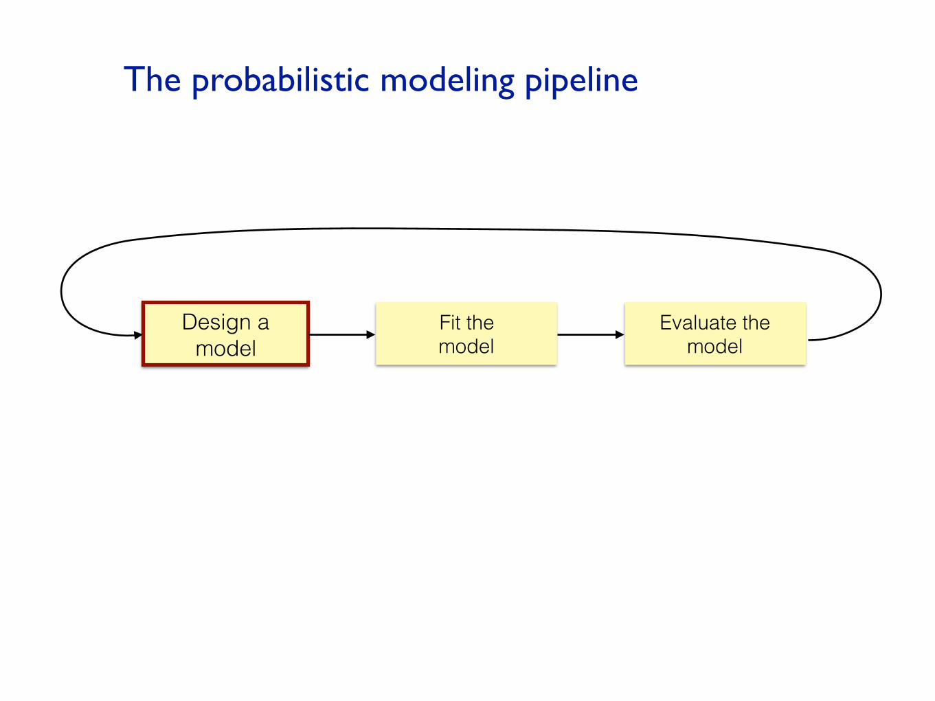
The probabilistic modeling pipeline
Design a model
Fit the model
Evaluate the model
Can we identify good models automatically?
Two challenges:
Automating each stage of this pipeline
Identifying a promising set of candidate models

The probabilistic modeling pipeline
Design a model
Fit the model
Evaluate the model
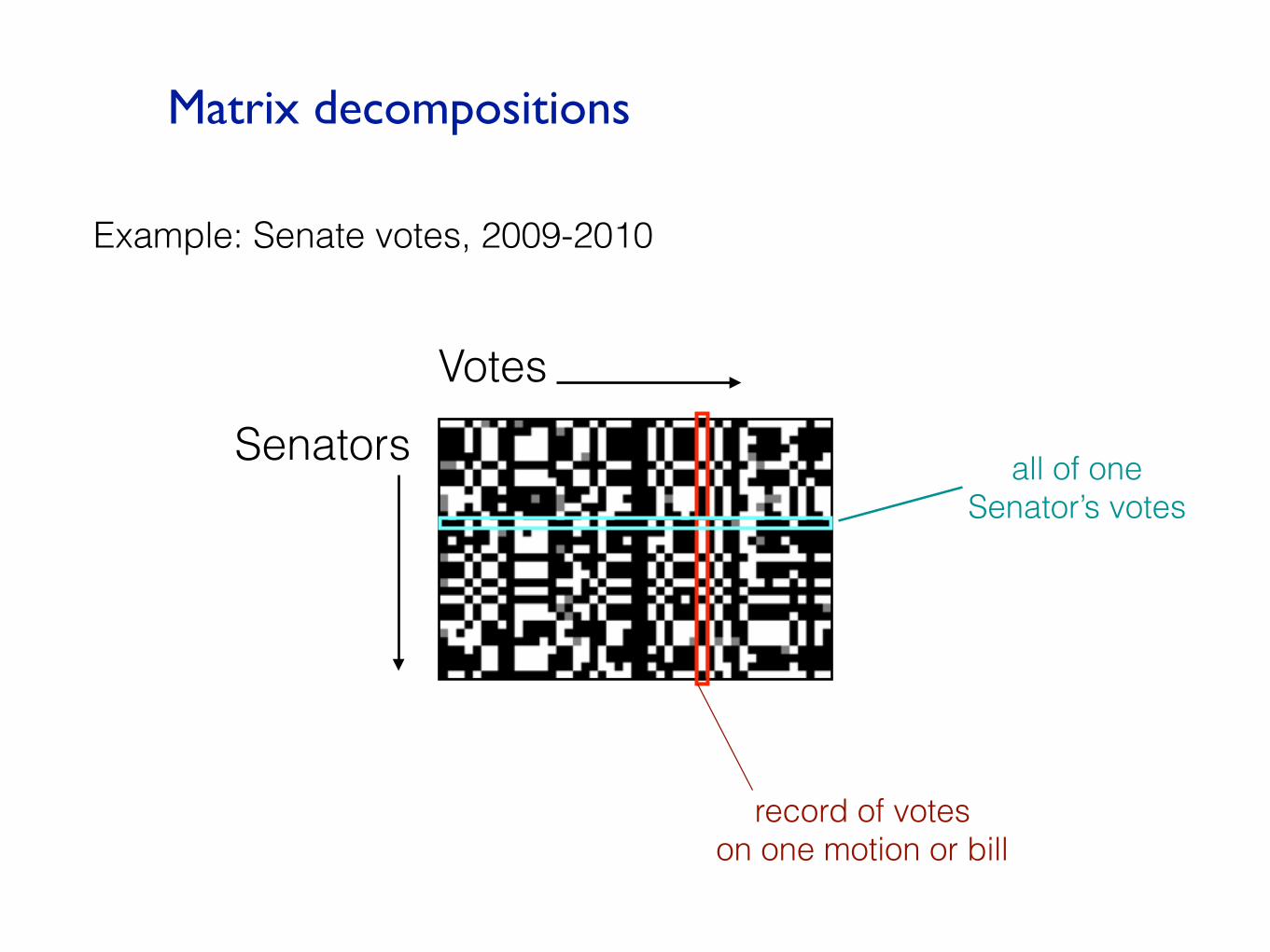
Matrix decompositions
VotesSenators all of one
Senator’s votes
record of votes on one motion or bill
Example: Senate votes, 2009-2010
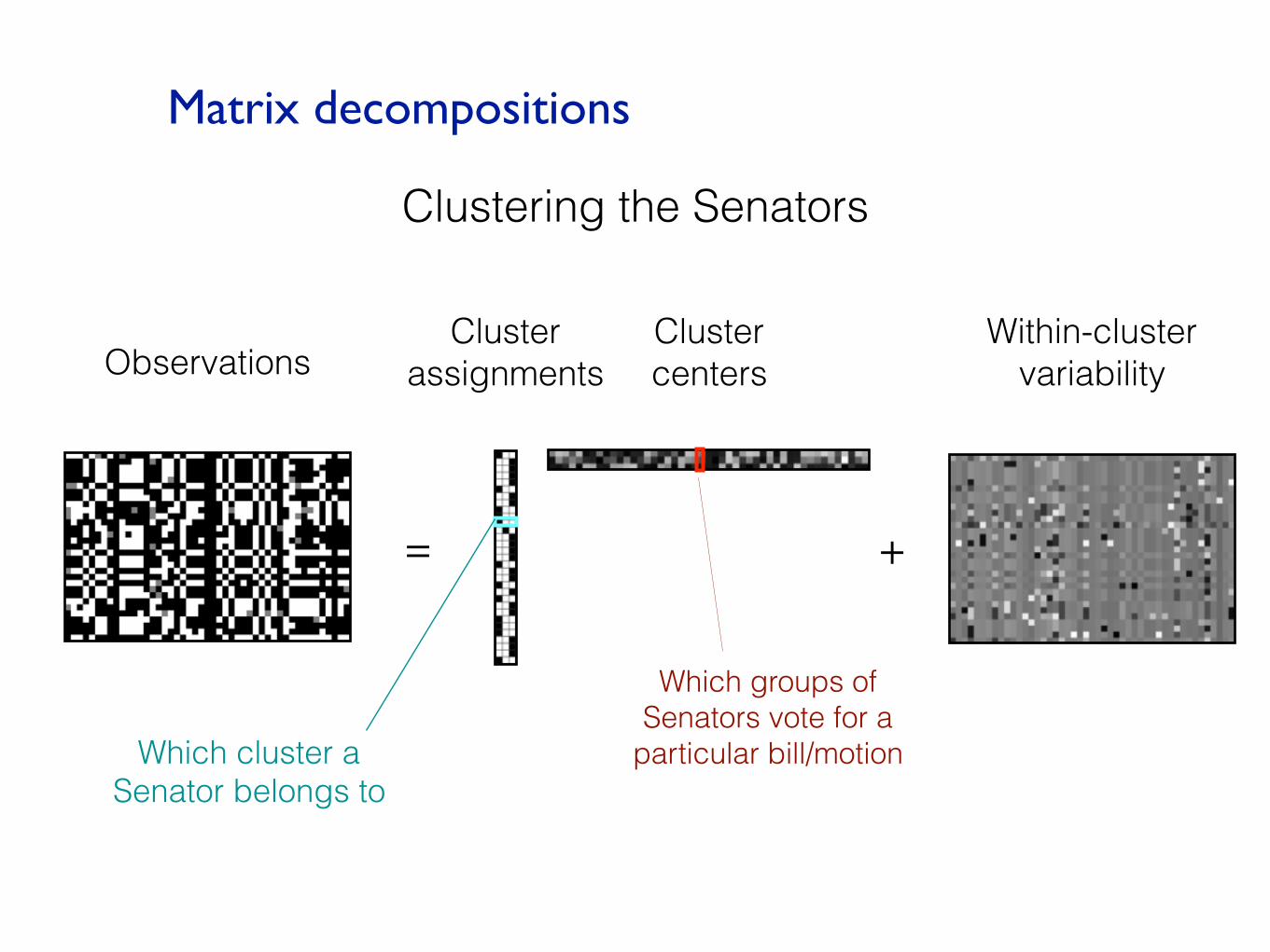
Matrix decompositions
= +
Clustering the Senators
ObservationsCluster centers
Cluster assignments
Within-cluster variability
Which groups of Senators vote for a
particular bill/motionWhich cluster a Senator belongs to
Matrix decompositions
= +
Clustering the Senators
ObservationsCluster centers
Cluster assignments
Within-cluster variability

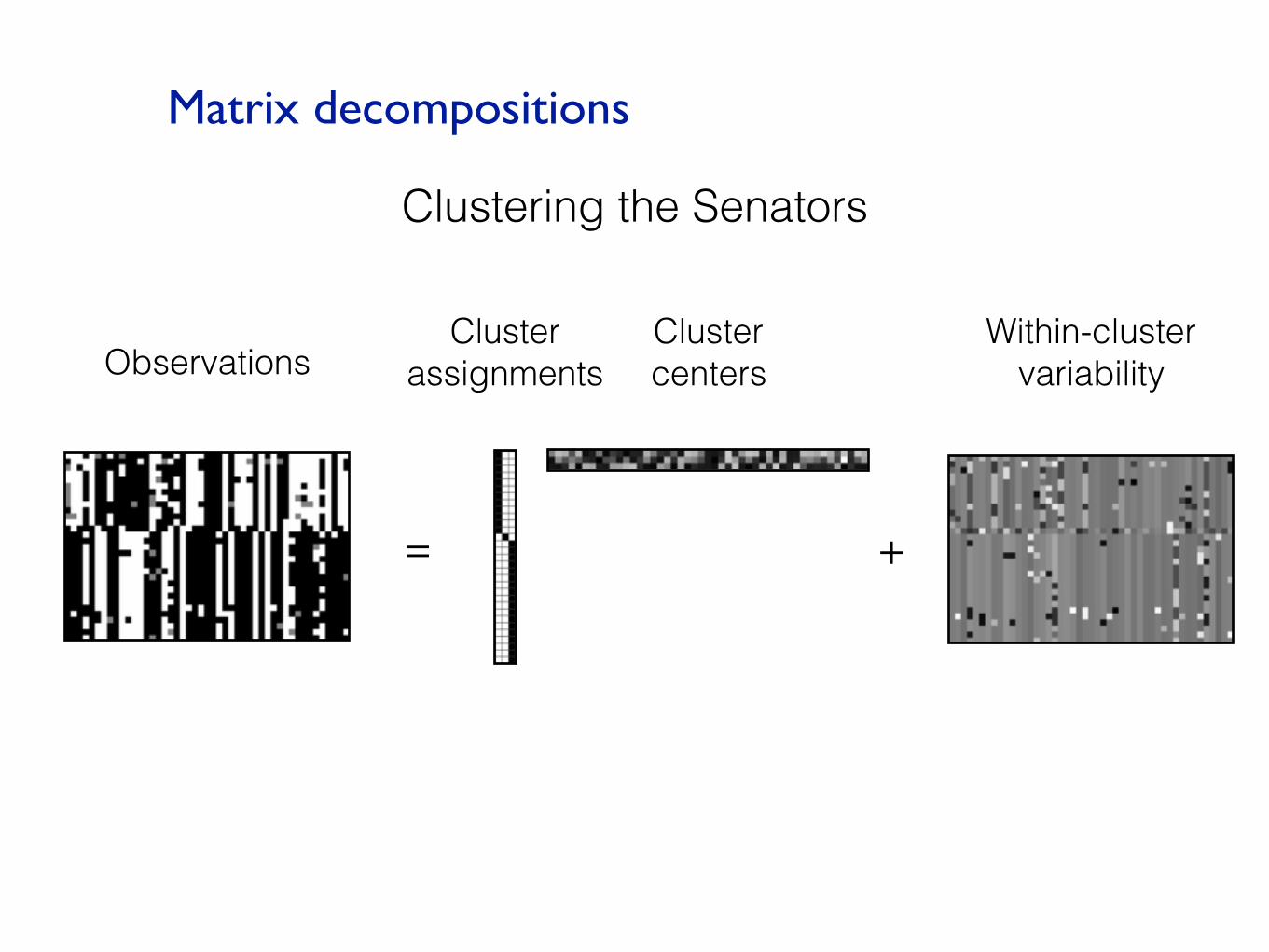
Matrix decompositions
= +
Clustering the votes
ObservationsCluster centers
Cluster assignments
Within-cluster variability
which cluster a vote belongs to
which Senators tend to vote for one sort of
bill/motion
what sorts of bills/motions one Senator tends to
vote for

Matrix decompositions
= +
Clustering the votes
ObservationsCluster centers
Cluster assignments
Within-cluster variability
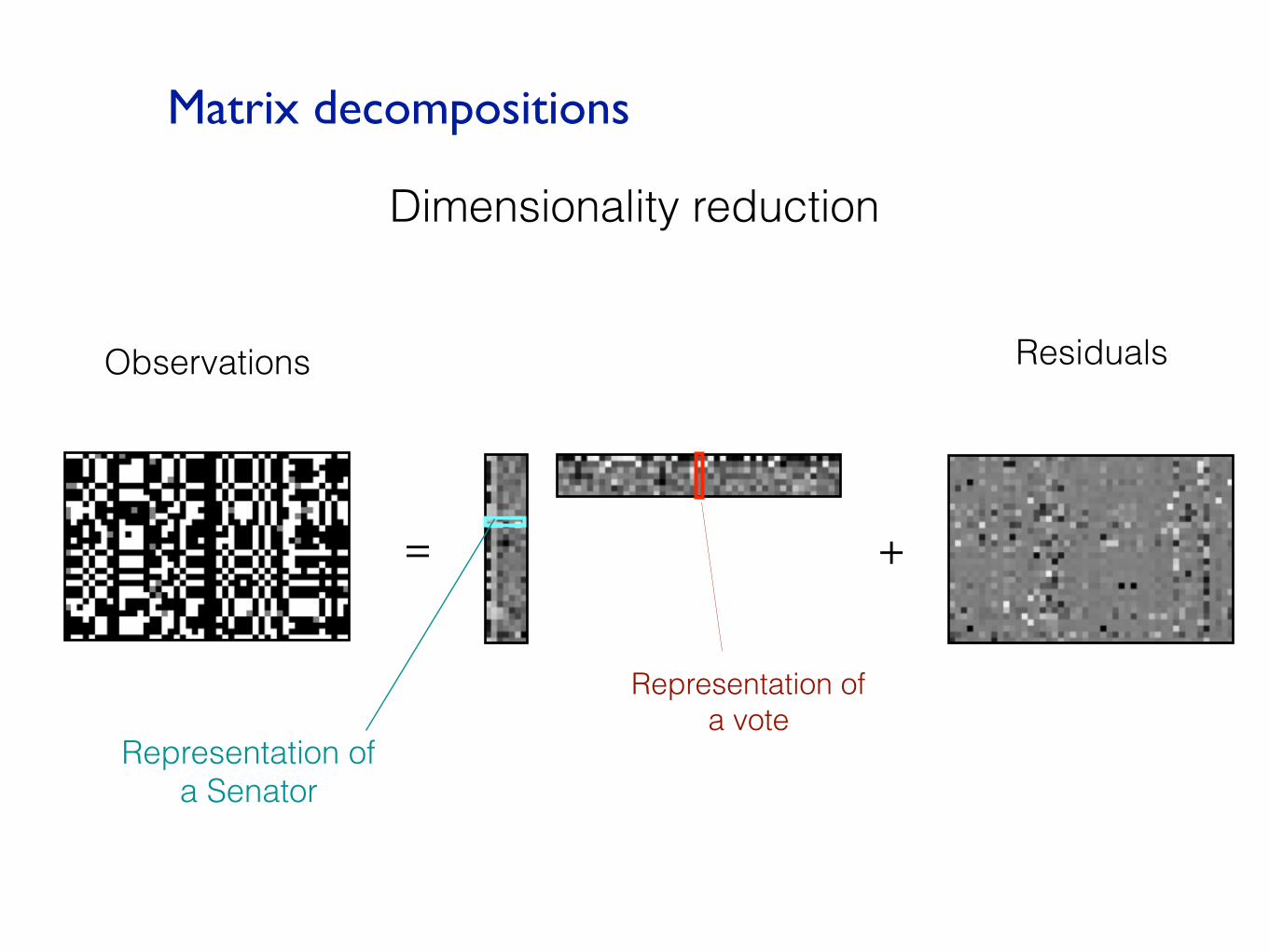
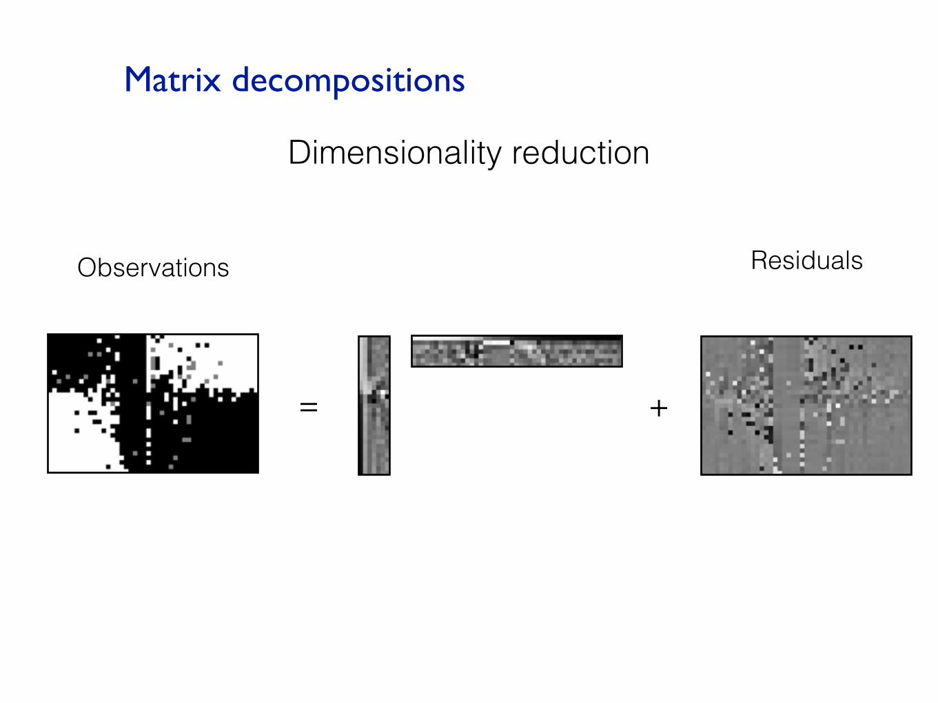
Matrix decompositions
= +
Dimensionality reduction
Observations Residuals
Representation of a vote
Representation of a Senator
Matrix decompositions
= +
Dimensionality reduction
Observations Residuals
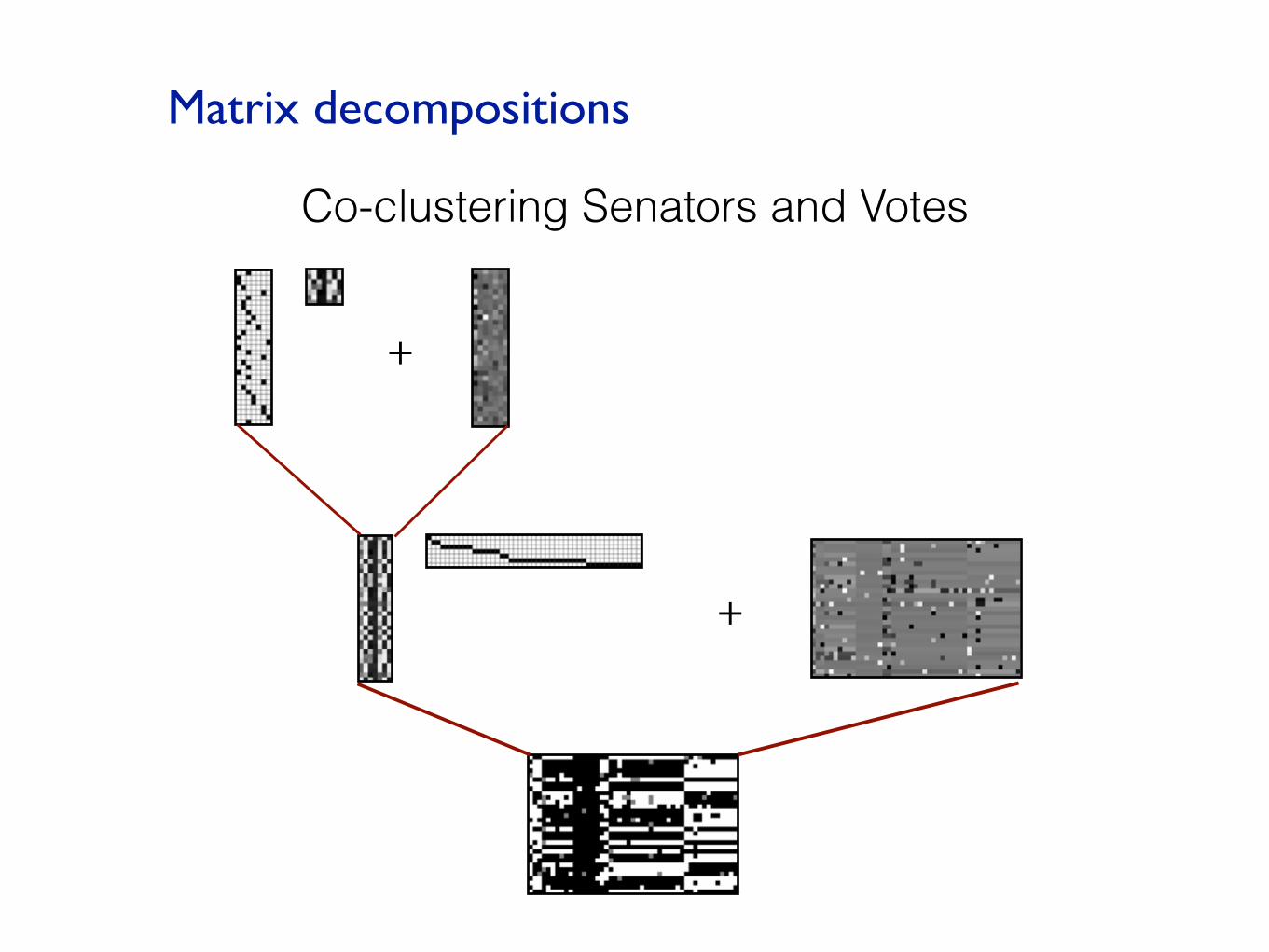
Matrix decompositions
Co-clustering Senators and Votes
+
+

Matrix decompositions
Co-clustering Senators and Votes
+
+

Matrix decompositions
…
No structure Cluster columns Cluster rows
Dimensionality reduction Co-clustering
The probabilistic modeling pipeline
Design a model
Fit the model
Evaluate the model

Building models compositionally
We build models by composing simpler motifs
Clustering Dimensionalityreduction Binary attributes
Heavy-taileddistributions
xxx xx
xx
xxx
x
x
x
xx
x
x
x xxxx x
xx
xxx
xx x
xx
xx x
xxx
x
PeriodicitySmoothness
+ - - ++ + +
++ +
-- - -
- -
x x
xx
x xx
x
x
xx
x x
x x

(Ghahramani, 1999 NIPS tutorial)
Building models compositionally
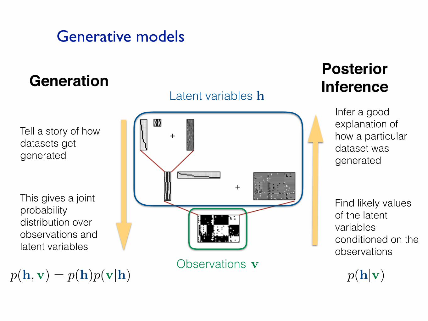
Generative models
GenerationPosteriorInference
Tell a story of how datasets get generated
This gives a joint probability distribution over observations and latent variables
Infer a good explanation of how a particular dataset was generated
Find likely values of the latent variables conditioned on the observations
Observations
Latent variables
v
h
p(h,v) = p(h)p(v|h) p(h|v)

Space of models: building blocks
Gaussian(G)
Multinomial(M)
Bernoulli (B)
Integration(C)
�i � Gamma(a, b)�j � Gamma(a, b)
uij � Normal(0,��1i ��1
j )
� � Dirichlet(�)ui � Multinomial(�)
pj � Beta(�, �)uij � Bernoulli(pj)
uij =�
1 if i � j0 otherwise
Grosse, Salakhutdinov, Freeman, and Tenenbaum, UAI 2012

Space of models: generative process
M G G+
MT + G
1. Sample all leaf matrices independently from their corresponding prior distributions
2. Evaluate the resulting expression
We represent models as algebraic expressions.
Grosse, Salakhutdinov, Freeman, and Tenenbaum, UAI 2012

Space of models: grammar
Gaussian(G)
Multinomial(M)
Bernoulli (B)
Integration(C)
Production rules:
GStarting symbol:
clustering G � MG + G | GMT + GM � MG + G
low rank G � GG + Gbinary features G � BG + G | GBT + G
B � BG + GM � B
linear dynamics G � CG + G | GCT + Gsparsity G � exp(G) �G
clustering G � MG + G | GMT + GM � MG + G
low rank G � GG + Gbinary features G � BG + G | GBT + G
B � BG + GM � B
linear dynamics G � CG + G | GCT + Gsparsity G � exp(G) �G
clustering G � MG + G | GMT + GM � MG + G
low rank G � GG + Gbinary features G � BG + G | GBT + G
B � BG + GM � B
linear dynamics G � CG + G | GCT + Gsparsity G � exp(G) �G
clustering G � MG + G | GMT + GM � MG + G
low rank G � GG + Gbinary features G � BG + G | GBT + G
B � BG + GM � B
linear dynamics G � CG + G | GCT + Gsparsity G � exp(G) �G
clustering G � MG + G | GMT + GM � MG + G
low rank G � GG + Gbinary features G � BG + G | GBT + G
B � BG + GM � B
linear dynamics G � CG + G | GCT + Gsparsity G � exp(G) �G
Grosse, Salakhutdinov, Freeman, and Tenenbaum, UAI 2012

M G +
GMT +
GExample: co-clustering
G
G MT G+
Grosse, Salakhutdinov, Freeman, and Tenenbaum, UAI 2012
G� GM� + GG�MG + G

Examples from the literature
no structure
clustering
co-clustering(e.g. Kemp et al., 2006) binary features
(Griffiths and Ghahramani, 2005)
sparse coding (e.g. Olshausen and Field, 1996)
low-rank approximation(Salakhutdinov and
Mnih, 2008)
Bayesian clustered tensor factorization (Sutskever et al., 2009)
binary matrix factorization(Meeds et al., 2006)
random walk
linear dynamical system
dependent gaussian scale mixture(e.g. Karklin and Lewicki, 2005)
......
......
Figure 2: Examples of existing machine learning models which fall under our framework. Arrows represent models reachable using asingle production rule. Only a small fraction of the 2496 models reachable within 3 steps are shown, and not all possible arrows areshown.
smart initialization step is followed by generic Gibbs sam-pling over the entire model. We note that our initializationprocedure generalizes “tricks of the trade” whereby com-plex models are initialized from simpler ones (Kemp et al.,2006; Miller et al., 2009).
In addition to simplifying the engineering, this procedureallows us to reuse computations between different struc-tures. Most of the computation time is in the initializationsteps. Each of these steps only needs to be run once on thefull matrix, specifically when the first production rule is ap-plied. Subsequent initialization steps are performed on thecomponent matrices, which are considerably smaller. Thisallows a large number of high level structures to be fit for afraction of the cost of fitting them from scratch.
5 Scoring candidate structures
Performing model selection requires a criterion for scoringindividual structures which is informative yet tractable. Tomotivate our method, we first discuss two popular choices:marginal likelihood of the input matrix and entrywise meansquared error (MSE). Marginal likelihood, the probabilityof the data with all the latent variables integrated out, iswidely used in Bayesian model selection. Unfortunately,this requires integrating out all of the latent component ma-trices, whose posterior distribution is highly complex andmultimodal. While elegant solutions exist for particularmodels, estimating the data marginal likelihood genericallyis still extremely difficult. At the other extreme, one canhold out a subset of the entries of the matrix and computethe mean squared error for predicting these entries. MSEis easier to implement, but we found that it was unable todistinguish many of the the more complex structures in ourgrammar.
As a compromise between these two approaches, we choseto evaluate predictive likelihood of held-out rows and
columns. That is, for each row (or column) x of the matrix,we evaluate p(x|XO), where XO denotes an “observed”sub-matrix. Like marginal likelihood, this tests the model’sability to predict entire rows or columns. However, it canbe efficiently approximated in our class of models usinga small but carefully chosen toolbox corresponding to thecomponent matrix priors in our grammar. We discuss thecase of held-out rows; columns are handled analogously.
First, by expanding out the products in the expression, wecan write the decomposition uniquely in the form
X = U
1
V
1
+ · · ·+ UnVn + E, (1)
where E is an i.i.d. Gaussian “noise” matrix and the Ui’sare any of the following: (1) a component matrix G, M ,or B, (2) some number of Cs followed by G, (3) a Gaus-sian scale mixture. The held-out row x can therefore berepresented as:
x = V
T1
u
1
+ · · ·+ V
Tn un + e. (2)
The predictive likelihood is given by:
p(x|XO) =
Zp(UO, V |XO)p(u|UO)p(x|u, V ) dUO du dV
(3)
where UO is shorthand for (UO1
, . . . , UOn) and u is short-hand for (u
1
, . . . , un).
In order to evaluate this integral, we generate samples fromthe posterior p(UO, V |X) using the techniques describedin Section 4, and compute the sample average of
ppred(x) ,Z
p(u|UO)p(x|u, V ) du (4)
If the term Ui is a Markov chain, the predictive distribu-tion p(ui|UO) can be computed using Rauch-Tung-Striebelsmoothing; in the other cases, u and UO are related only
Grosse, Salakhutdinov, Freeman, and Tenenbaum, UAI 2012

The probabilistic modeling pipeline
Design a model
Fit a model
Evaluate the model
Posterior Inference

Algorithms: posterior inference
Recursive initializationfit a clustering
model
Grosse, Salakhutdinov, Freeman, and Tenenbaum, UAI 2012
implement one algorithm per production rule
share computation between models
Choose the model dimension using Bayesian nonparametrics
G�MG + G
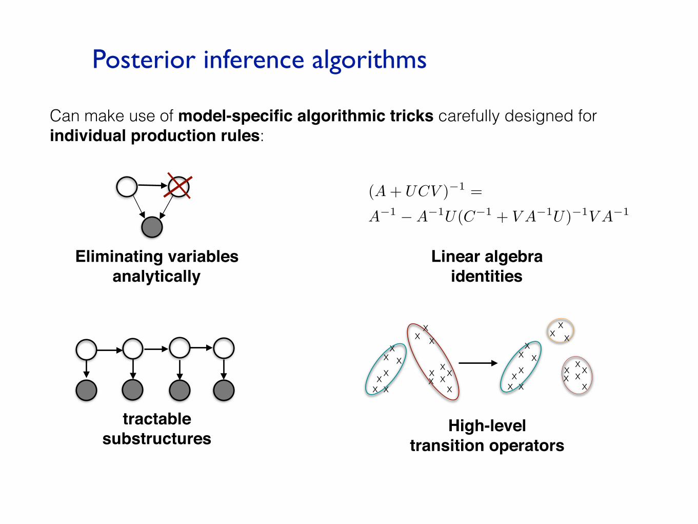
Posterior inference algorithms
Can make use of model-specific algorithmic tricks carefully designed for individual production rules:
High-leveltransition operators
Linear algebraidentities
(A + UCV )�1 =
A�1 �A�1U(C�1 + V A�1U)�1V A�1
tractablesubstructures
Eliminating variablesanalytically
x xxx
x xx
xxx
xx xxx
x x xxx
x xx
xxx
xx xxx
x

The probabilistic modeling pipeline
Design a model
Fit a model
Evaluate the model
We evaluate models on the probability they assign to held-out subsets of the observation matrix.

The probabilistic modeling pipeline
Design a model
Fit a model
Evaluate the model
Want to search over the large, open-ended space of models
Key problem: the search space is very large!
over 1000 models reachable in 3 productions
how to choose a promising set of models to evaluate?

Algorithms: structure search
Model patches as linear combinations of uncorrelated
basis functions
Fourier representation
Sanger, 1988 Olshausen and Field, 1994
Model the heavy-tailed distributions of coefficients
oriented edges similar to simple cells
Karklin and Lewicki, 2005, 2008
Model the dependencies between scales of
coefficients
high-level texture representation similar
to complex cells
A brief history of models of natural images…
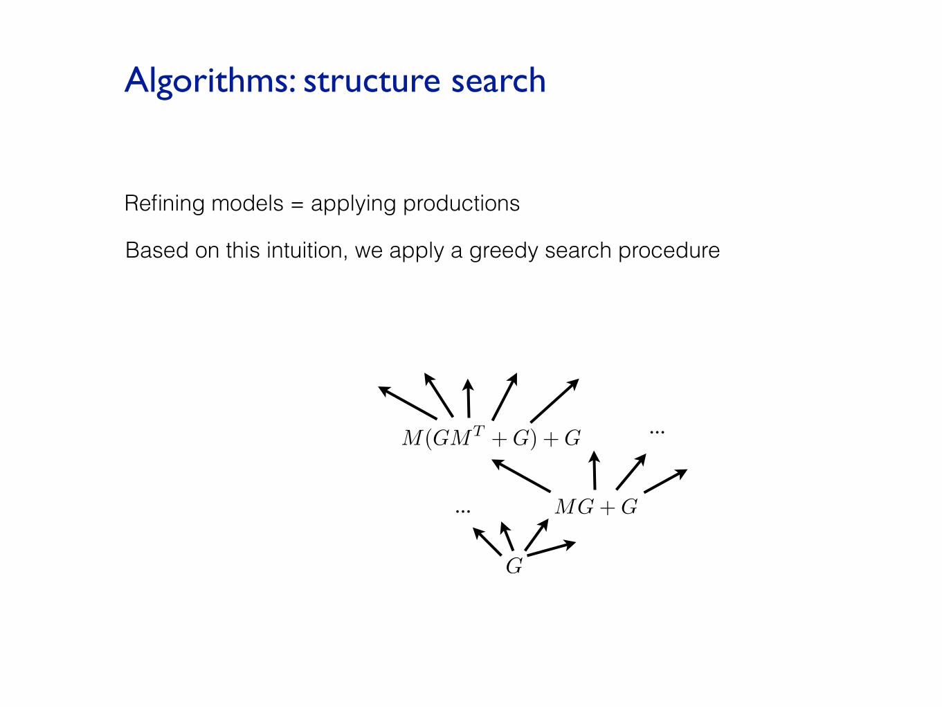
Algorithms: structure search
Refining models = applying productions
Based on this intuition, we apply a greedy search procedure
...
...
G
MG + G
M(GMT + G) + G
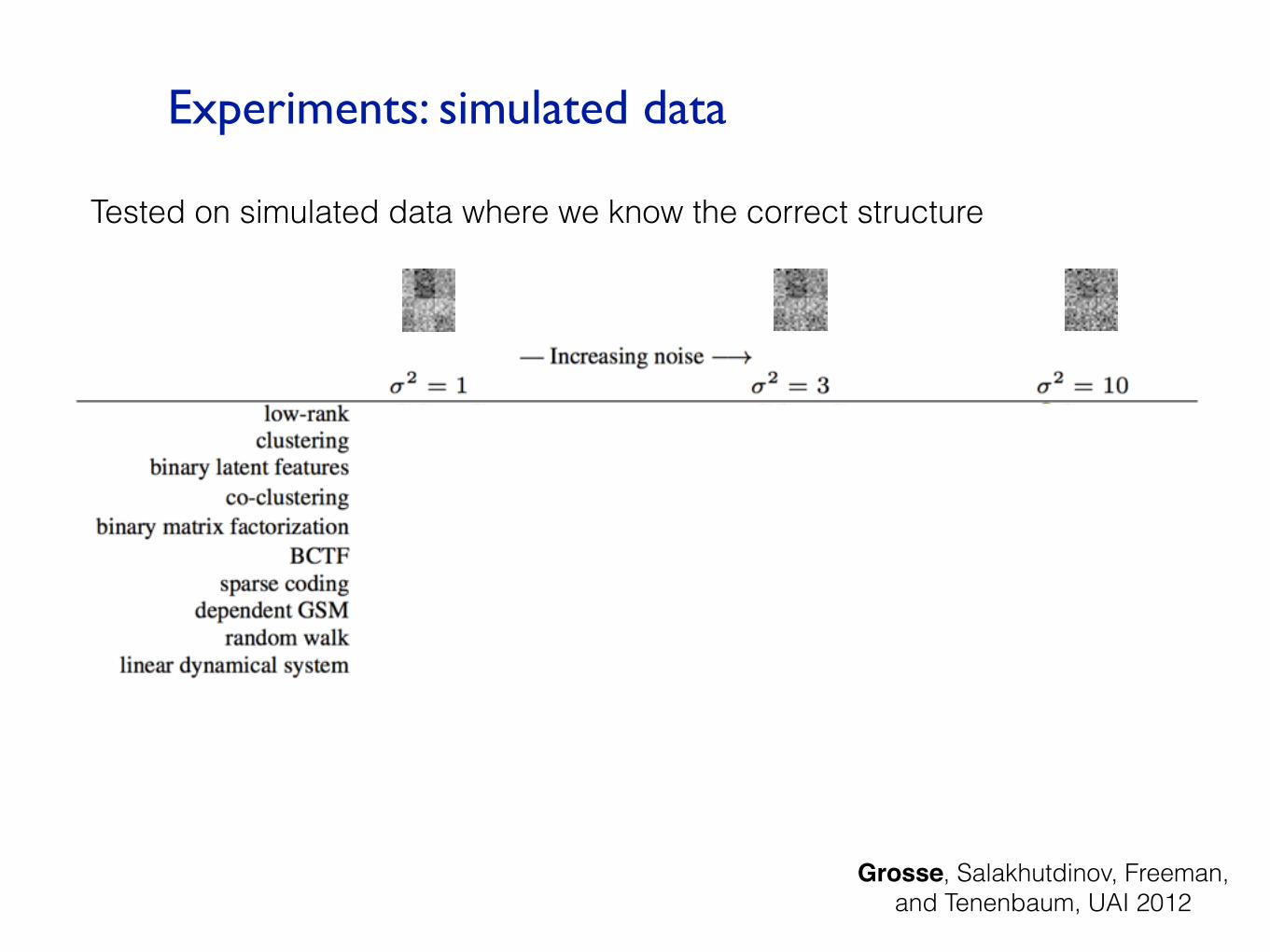
Experiments: simulated data
Tested on simulated data where we know the correct structure
Grosse, Salakhutdinov, Freeman, and Tenenbaum, UAI 2012

Experiments: simulated data
Tested on simulated data where we know the correct structure
Usually chooses the correct structure in low-noise conditions
Grosse, Salakhutdinov, Freeman, and Tenenbaum, UAI 2012

Experiments: simulated data
Tested on simulated data where we know the correct structure
Usually chooses the correct structure in low-noise conditions
Gracefully falls back to simpler models under heavy noise
Grosse, Salakhutdinov, Freeman, and Tenenbaum, UAI 2012

Experiments: real-world data
Senate votes 09-10 GMT + G —(MG + G)MT + G
Cluster votes.
22 clusters
largest: party line Democrat, party line Republican, all yea
others are series of votes on single issues
Cluster Senators.
11 clusters
no cross-party clustersNo third level model improves by more than 1 nat
Grosse, Salakhutdinov, Freeman, and Tenenbaum, UAI 2012

Experiments: real-world data
Senate votes 09-10 GMT + G —(MG + G)MT + G
CG + G C(GG + G) + GMotion capture —
Data: motion capture of a person walking. Each row gives a person’s displacement and joint angles in one frame.
Model 1: Independent Markov chains
Model 2: Correlations in joint angles
Grosse, Salakhutdinov, Freeman, and Tenenbaum, UAI 2012
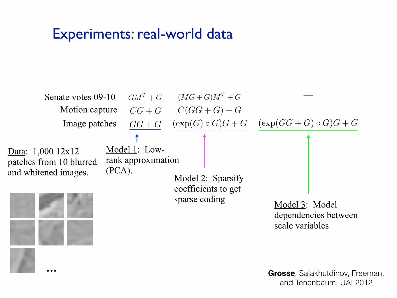
Experiments: real-world data
Senate votes 09-10 GMT + G —(MG + G)MT + G
CG + G C(GG + G) + GMotion capture —
Data: 1,000 12x12 patches from 10 blurred and whitened images.
Model 1: Low-rank approximation (PCA).
Model 2: Sparsify coefficients to get sparse coding Model 3: Model
dependencies between scale variables
...
GG + G (exp(G) � G)G + G (exp(GG + G) � G)G + GImage patches
Grosse, Salakhutdinov, Freeman, and Tenenbaum, UAI 2012

Experiments: real-world data
Senate votes 09-10 GMT + G —(MG + G)MT + G
CG + G C(GG + G) + GMotion capture —GG + G (exp(G) � G)G + G (exp(GG + G) � G)G + GImage patches
Data: Mechanical Turk users’ judgments to 218 questions about 1000 entities
Model 1: Cluster entities.
39 clusters
Model 2: Low-rank representation of cluster centers.
8 dimensions
Dimension 1: living vs. nonliving
Dimension 2: large vs. small
—Concepts MG + G M(GG + G) + G
Grosse, Salakhutdinov, Freeman, and Tenenbaum, UAI 2012

“Structure discovery in nonparametric regression through compositional kernel search,” ICML 2013.
David Duvenaud, James Lloyd, Roger Grosse, Josh Tenenbaum, and Zoubin Ghahramani,

Compositional structure search for time series
Lin� Lin SE�Per
Lin + Per Lin�Per
SE Per
Lin RQ
Primitive kernels: Composite kernels:
Gaussian processes are distributions over functions, specified by kernels.
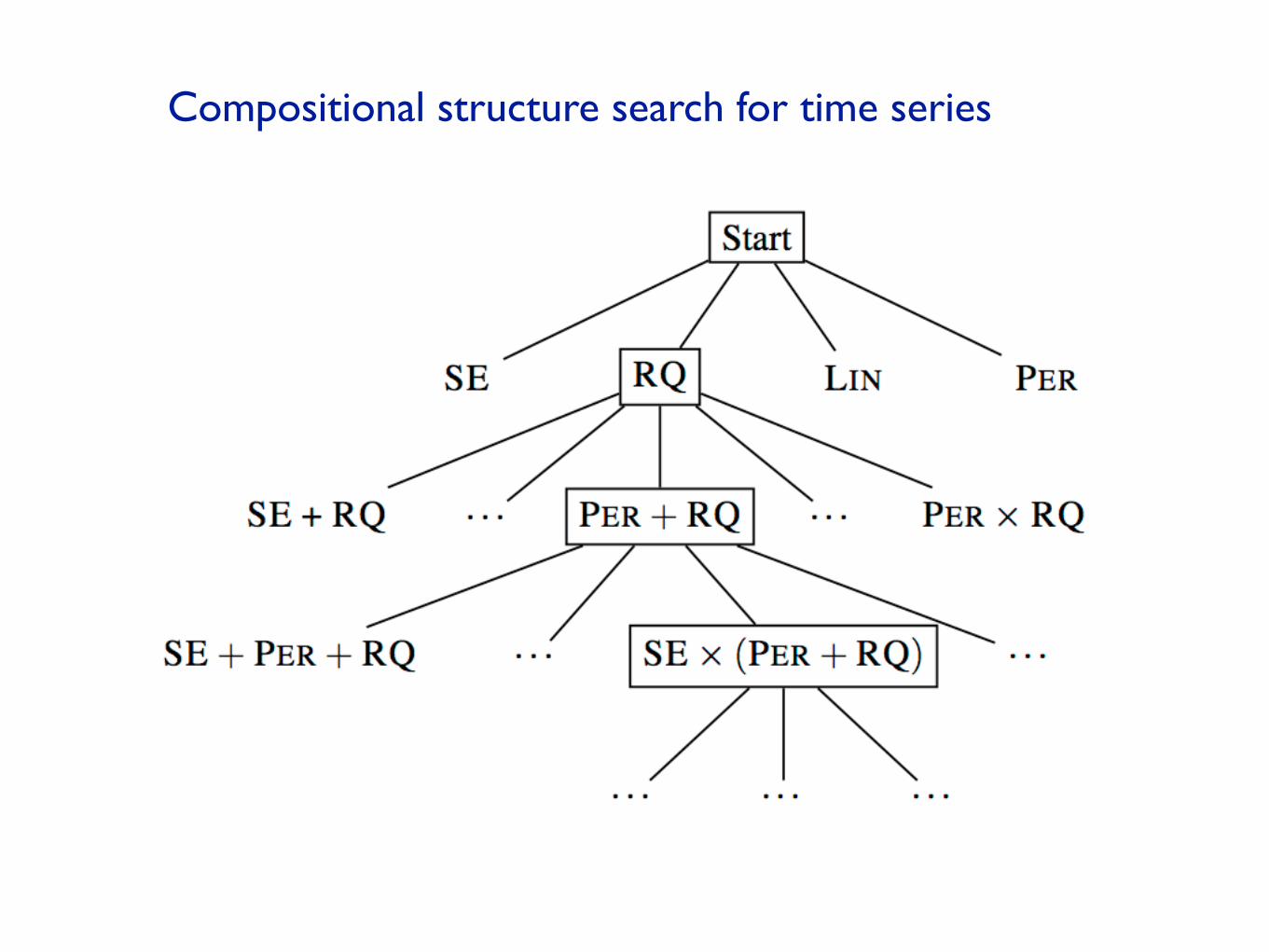
Compositional structure search for time series

Compositional structure search for time series
radio critical frequency

…

10 minute break