Explicit iteration MCS for random vibration of nonlinear...
37
Explicit iteration MCS for random vibration of nonlinear systems Cheng Su, Huan Huang, Haitao Ma School of Civil Engineering and Transportation South China University of Technology Guangzhou 510640, China December 12, 2014 The 6th Kwan-Hua Forum, Innovations and Implementations in Earthquake Engineering Research, December 12-14, 2014, Shanghai, China South China University of Technology
Transcript of Explicit iteration MCS for random vibration of nonlinear...

Explicit iteration MCS for random vibration
of nonlinear systems
Cheng Su, Huan Huang, Haitao Ma
School of Civil Engineering and Transportation
South China University of Technology
Guangzhou 510640, China
December 12, 2014
The 6th Kwan-Hua Forum, Innovations and Implementations in Earthquake
Engineering Research, December 12-14, 2014, Shanghai, China
South China University of Technology
Contents
1 Introduction
2 Explicit expressions of dynamic responses : linear systems
3 Explicit iteration MCS : nonlinear systems
4 Numerical examples
5 Concluding remarks
South China University of Technology

Method
Comparision from different points of view
1 2 3 4 5
Stationary Non-
stationary
Wide
band
Narrow
band
White
noise
Non-white
noise Gaussian
Non-
Gaussian
Small
number of
DOFs
Large
number of
DOFs
FPK equation
method √ × √ × √ × √ × √ ×
Stochastic
average
method
√ × √ × √ √ √ √ √ ×
Moment
equation
method
√ √ √ × √ × √ √ √ ×
Stochastic
perturbation
method
√ × √ √ √ √ √ √ √ ×
Equivalent
linearization
method
√ √ √ √ √ √ √ × √ √
Equivalent
nonlinear
system method
√ × √ × √ × √ × √ ×
Nonlinear random vibration analytical methods
1 Introduction
South China University of Technology

Contents
1 Introduction
2 Explicit expressions of dynamic responses : linear systems
3 Explicit iteration MCS : nonlinear systems
4 Numerical examples
5 Concluding remarks
South China University of Technology

1 1
where
t
t X t
( )
, ( ) ( )
0 I 0,
V HV P
YV P W
Y
H WM K M C E
State equation
Recurrence formula
1 1 1 2
2 1
1
2 1
2
1 2
where
e
i i i i
t
X X
i l
t
t
( , , , )
(I ) /
( I) /
H
V TV Q Q
T
Q T H W TH W
Q T H W H W
,0 0 ,1 1 ,
1,0 1
1,1 2
2,0 1,0
2,1 2 1
2,2 1,1
,0 1,0
,1 1,1
( 1, 2, , )
where
( 1)
( 2)
i i i i i i
i i
i i
X X X
i l
i
i
V A A A
A Q
A Q
A TA
A TQ Q
A A
A TA
A TA
, 1, 1
(3 )
(2 )i j i j
i l
j i
A A
Explicit expressions of dynamic
responses
( )MY CY KY MEX t
Motion Equation
( )
0( ) e (0) e ( )d
tt tt
H HV V P
Solution to state equation
Can also be obtained using
the other step-by-step
integration approaches
2 Explicit expressions of dynamic responses: linear systems
Ground acceleration
process

South China University of Technology
X
t1 t2 t3 t4
tt0
1
tl…A3,2
A4,2
A l,2
A2,2
Explicit expressions of dynamic responses
,0 0 ,1 1 , ( 1,2, , )i i i i i iX X X i l V A A A
The responses due to a
unit impulse at time t0 Vi=Ai,0 (i=1,2,3,…,l)
The responses due to a
unit impulse at time t2 Vi=Ai,2 (i=2,3,…,l)
X
t1 t2 t3 t4
tt0
1
tl…A1,0
A2,0
A3,0
A4,0
A l,0
X
t1 t2 t3 t4
tt0
1
tl…A2,1
A3,1
A4,1
A l,1
A1,1
A3,1
A l-1,1A1,1
A2,1
X 0 X 1 X 2 X 3 … X l- 2 X l- 1 X l
t 1 A 1,0 A 1,1
t 2 A 2,0 A 2,1 A 2,2
t 3 A 3,0 A 3,1 A 3,2 A 3,3
t 4 A 4,0 A 4,1 A 4,2 A 4,3
… … … … … …
t l -2 A l -2,0 A l -2,1 A l -2,2 A l -2,3 … A l -2,l -2
t l -1 A l -1,0 A l -1,1 A l -1,2 A l -1,3 … A l -1,l -2 A l -1,l -1
t l A l ,0 A l ,1 A l ,2 A l ,3… A l ,l -2 A l ,l -1 A l ,l
时刻系数向量
Time Coefficient matrices
The responses due to a
unit impulse at time t1 Vi=Ai,1 (i=1,2,3,…,l)
2 Explicit expressions of dynamic responses: linear systems

系数向量 时刻
0X 1X 2X 3X 2lX 1lX lX
1t 1,0A 1,1A
2t 2,0A 2,1A 1,1A
3t 3,0A 3,1A 2,1A 1,1A
2lt 2,0lA 2,1lA 3,1lA 4,1lA 1,1A
1lt 1,0lA 1,1lA 2,1lA 3,1lA 2,1A 1,1A
lt ,0lA ,1lA 1,1lA 2,1lA 3,1A 2,1A 1,1A
The same as those matrices in the second column
,0 0 ,1 1 , ( 1,2, , )i i i i i iX X X i l V A A A
Explicit expressions of dynamic responses
■Computational cost=Two deterministic time-history response analyses
■ Storage capacity=Storage of the first two columns of matrices
Time Coefficient matrices
Obtained by a deterministic time-history response analysis with a unit impulse at time t0
Obtained by a deterministic time-history response analysis with a unit impulse at time t1
South China University of Technology
C. Su et al., Acta Mech. Sinica, 2010, 42(3): 512-520
C. Su et al., Struct. Eng. Mech., 2014, 52 (2): 239-260
2 Explicit expressions of dynamic responses: linear systems
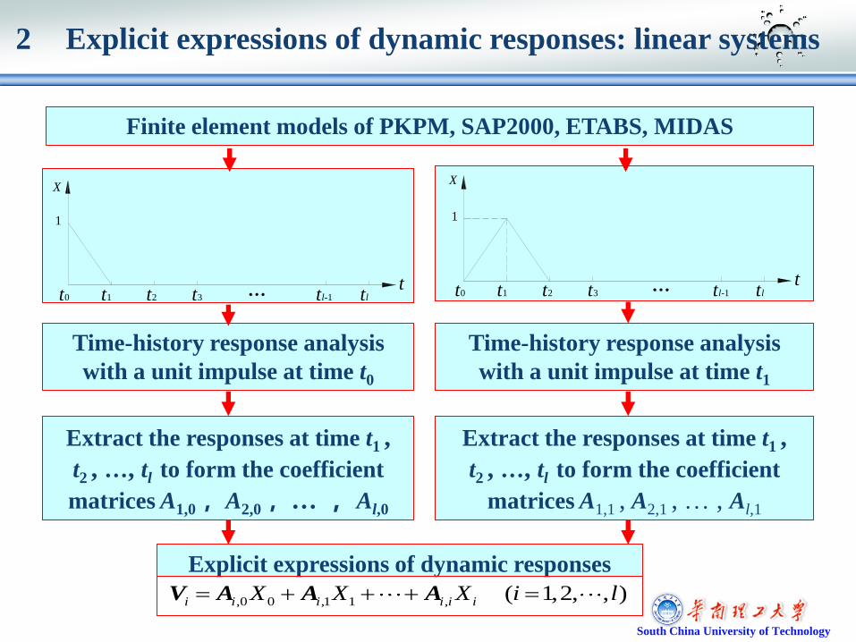
Extract the responses at time t1 ,
t2 , …, tl to form the coefficient
matrices A1,0, A2,0, … , Al,0
Time-history response analysis
with a unit impulse at time t1
Finite element models of PKPM, SAP2000, ETABS, MIDAS
Time-history response analysis
with a unit impulse at time t0
Extract the responses at time t1 ,
t2 , …, tl to form the coefficient
matrices A1,1 , A2,1 , … , Al,1
X
t1 t2 t3 tl-1
tt0
1
tl…
X
t1 t2 t3
tt0
1
tl… tl-1
South China University of Technology
,0 0 ,1 1 , ( 1,2, , )i i i i i iX X X i l V A A A
Explicit expressions of dynamic responses
2 Explicit expressions of dynamic responses: linear systems
1 Introduction
2 Explicit expressions of dynamic responses : linear systems
3 Explicit iteration MCS : nonlinear systems
4 Numerical examples
5 Concluding remarks
Contents
South China University of Technology

Dimension-
reduced
iteration
Quasi-linear motion equation
= ( )
( )= ( )- ( , )
MU CU KU F
F F f U U
t
t t
Explicit iteration for dynamic responses
(0)
-1
( ) ( 1)
,0 0 ,1 1 , -1 -1 ,
Initial values ( )= ( )
= + [ - ( )]
( =1,2, , ; =1,2, )
i i
j j
i i i i i i i i i i
i l j
-
:f V f V
V A F A F A F A F f V
( , ) ( ) MU CU KU f U U F t
Nonlinear motion equation
,0 0 ,1 1 , -1 -1 ,
=1,2, ,
i i i i i i i i i
i l
V A F A F A F A F
( )
Explicit expressions of dynamic
responses (in form)
1 (0) 1
-1
1 ( ) 1 1 1
,0 0 ,1 1 , -1 -1
1 1 ( -1)
,
2 2 2 2
,0 0 ,1 1 , -1 -1
2 1
,
Initial values ( )= ( )
=
+ [ - ( )]
=
+ [ - ( )]
i i
j
i i i i i i
j
i i i i
i i i i i i
i i i i
:f V f V
V A F A F A F
A F f V
V A F A F A F
A F f V
( =1,2, , ; =1,2, )i l j
Dimension-reduced iteration process
DOFs
associated with
nonlinear terms
DOFs
non-associated
with nonlinear
terms
3 Explicit iteration MCS : nonlinear systems
South China University of Technology

DOFs
associated with
nonlinear terms
( ) ( =1,2, , )Fk t k N
N samples of non-stationary
random excitation
( , ) ( )
( =1,2, , )
MU CU KU f U U Fk k k k k k t
k N
Nonlinear motion equation
1 (0) 1
, , -1
1 ( ) 1 1 1 1 1 ( -1)
, ,0 ,0 ,1 ,1 , -1 , -1 , , ,
2 2 2 2 2 1
, ,0 ,0 ,1 ,1 , -1 , -1 , , ,
Initial values ( )= ( )
= + [ - ( )]
= + [ - ( )]
k i k i
j j
k i i k i k i i k i i i k i k i
k i i k i k i i k i i i k i k i
:f V f V
V A F A F A F A F f V
V A F A F A F A F f V
( =1,2, , ; =1,2, ; =1,2, , )i l j k N
Dimension-reduced iteration for the kth sample analysis
Calculated only once and remain the
same throughout the solution process
Dimension-
reduced iteration
DOFs
non-associated
with nonlinear
terms
3 Explicit iteration MCS : nonlinear systems
South China University of Technology

1 Introduction
2 Explicit expressions of dynamic responses : linear systems
3 Explicit iteration MCS : nonlinear systems
4 Numerical examples
5 Concluding remarks
Contents
South China University of Technology

ETABS FE model: 103 storeys, a total height of 432m, 19,813 nodes, 18,597 beam
elements, 14,074 shell elements, and a total number of DOFs of 154,583
Maximum value of response spectrum αmax=0.08, ground predominant period Tg=0.35s,
the first three natural periods T1=7.29s (y-direction), T2=7.21s (x-direction), T3=2.67s
(torsion)
4 Numerical examples (1) : Linear system
South China University of Technology

4 Numerical examples (1) : Linear system
South China University of Technology

Time elapsed by the present method
Total number
of DOFs
Elapsed time of
two time-history
response analyses
(ETABS)
Number of
responses
Number of
samples
Elapsed time of
random
simulation
154,583 21 min 10 sec 207 1,000 4 min 4 sec
4 Numerical examples (1) : Linear system
South China University of Technology

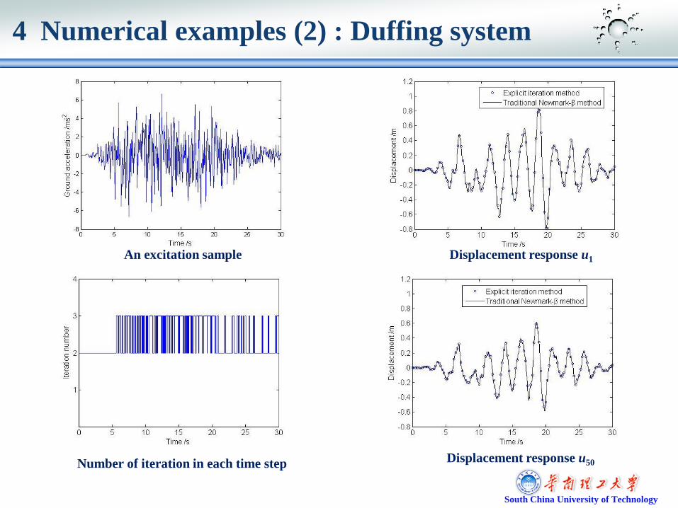
4 Numerical examples (2) : Duffing system
1 2 50
51 52 100
7
1 2 50
7
51 52 100
1 50 51 100
= =2500kg,
= = = =3000kg;
7.5 10 kN/m,
8 10 kN/m;
533.3, 500.0;
Damping ration 0.05 for the initial linear system
m m m
m m m
k k k
k k k
=
Structural parameters
31 21 1 1 1
3 32 32 2 2 1 1 1 2
3 33 43 3 3 2 2 2 3
3 399 10099 99 99 98 98 98 99
3 3100100 100 100 99 99 99 100
f ,
u uk y y
u uk y k y y
u uk y k y y
u uk y k y y
uk y k y y
Nonlinear restoring forces
100-DOF Duffing system
1u
2u
99u
100u
South China University of Technology C. Su et al., J. Vib. Eng., 2014, 27(2): 1-7

4 Numerical examples (2) : Duffing system
100-DOF Duffing system
1u
2u
99u
100u
4 2 2 2
02 2 2 2 2 2
2 3
0
4 ( )
( ) 4
where
15.708rad/s, 0.6, 0.05m / s
g g g
x
g g g
g g
S S
S
Kanai-Tajimi Spectrum for ground
acceleration
1 1
1 2
( )
2 3
1 2 3
( / ) 0
( ) 1
where
6.0s 18.0s 30.0s 0.18
2
2
-a t -t
t t t t
g t t t t
e t t t
t t t a
, , ,
Uniform modulation function for non-
stationary ground motion
South China University of Technology C. Su et al., J. Vib. Eng., 2014, 27(2): 1-7
South China University of Technology
Displacement response u1
Displacement response u50
4 Numerical examples (2) : Duffing system
An excitation sample
Number of iteration in each time step

South China University of Technology
Standard deviation of displacement u1
Standard deviation of displacement u50
Evolutionary PDF of displacement u1
Evolutionary PDF of displacement u50
4 Numerical examples (2) : Duffing system

Time elapsed by analysis of 100-DOF system
Time elapsed by analysis of 1,000-DOF system
South China University of Technology
4 Numerical examples (2) : Duffing system

First-order dynamic eigenvalue
Second-order dynamic eigenvalue
Third-order dynamic eigenvalue
Dynamic eigenvalues at t=18.55s (s-2)
4 Numerical examples (2) : Duffing system
South China University of Technology

South China University of Technology
100-DOF Duffing system
with local nonlinearities
1 2 50 51 52 100
7
1 2 50
7
51 52 100
90 100
= =2500kg, = = = =3000kg;
7.5 10 kN/m,
8 10 kN/m;
1000.0;
Damping ration 0.05 for the initial linear system
m m m m m m
k k k
k k k
=
Structural parameters
Nonlinear restoring forces
1 1 2
2 2 3
3
90 90 90 90 90 91
391 9290 90 90 91
3100100100 100 100
0
0
y u u
y u u
k y y u u
u uk y y
uyk y
f ,
Coefficients
of
nonlinear
restoring
forces
( )g
X t
4 Numerical examples (3) : Duffing system with local nonlinearities
DOFs
associated with
nonlinear terms

South China University of Technology
( )g
X t
4 2 2 2
02 2 2 2 2 2
2 3
0
4 ( )
( ) 4
where
15.708rad/s, 0.6, 0.05m / s
g g g
x
g g g
g g
S S
S
Kanai-Tajimi Spectrum for ground
acceleration
1 1
1 2
( )
2 3
1 2 3
( / ) 0
( ) 1
where
6.0s 18.0s 30.0s 0.18
2
2
-a t -t
t t t t
g t t t t
e t t t
t t t a
, , ,
Uniform modulation function for non-
stationary ground motion
100-DOF Duffing system
with local nonlinearities
4 Numerical examples (3) : Duffing system with local nonlinearities
Coefficients
of
nonlinear
restoring
forces
DOFs
associated with
nonlinear terms

Number of iteration in each time step
Displacement response u1
Displacement response u50
An excitation sample
4 Numerical examples (3) : Duffing system with local nonlinearities

South China University of Technology
Standard deviation of displacement u1
Standard deviation of displacement u50
Evolutionary PDF of displacement u1
Evolutionary PDF of displacement u50
4 Numerical examples (3) : Duffing system with local nonlinearities

Dynamic eigenvalues at t=18.55s (s-2)
First-order dynamic eigenvalue
Second-order dynamic eigenvalue
Third-order dynamic eigenvalue
South China University of Technology
4 Numerical examples (3) : Duffing system with local nonlinearities

Time elapsed by analysis of 100-DOF system
Time elapsed by analysis of 1,000-DOF system
South China University of Technology
4 Numerical examples (3) : Duffing system with local nonlinearities

1 2 50
51 52 100
7
1 2 50
7
51 52 100
= =6000kg,
= = = =5000kg;
8 10 kN/m,
7.5 10 kN/m;
Damping ration 0.05 for the initial linear system
m m m
m m m
k k k
k k k
=
Structural parameters
Hysteretic restoring forces
1
1 1
( , ) (1 )( 1,2, ,100)
| | | | | |
where
0.2 1 400m =300m
1 ( 1,2, ,100)
i i
i i i i i i i i i
i i i i i i i i i i
i i i i
i
f y z k y k zi
z A y y z z y z
A
i
, , , ,
An n-storey shear structure
( )g
X t
4 Numerical examples (4) : hysteretic system
South China University of Technology C. Su et al., Earthq. Struct., 2014, 7(2): 119-139

( )g
X t
4 Numerical examples (4) : hysteretic system
4 2 2 2
02 2 2 2 2 2
3 2 3
0
4 ( )
( ) 4
where
15.708rad/s, 0.6, 1.574 10 m / s
g g g
x
g g g
g g
S S
S
Kanai-Tajimi Spectrum for ground
acceleration
1 1
1 2
( )
2 3
1 2 3
( / ) 0
( ) 1
where
6.0s 18.0s 30.0s 0.18
2
2
-a t -t
t t t t
g t t t t
e t t t
t t t a
, , ,
Uniform modulation function for non-
stationary ground motion
South China University of Technology C. Su et al., Earthq. Struct., 2014, 7(2): 119-139
An n-storey shear structure

An excitation sample
Number of iteration in each time step
Displacement response u50
Displacement response u100
4 Numerical examples (4) : hysteretic system
South China University of Technology

Standard deviation of displacement u50
Standard deviation of displacement u100
Evolutionary PDF of displacement u50
Evolutionary PDF of displacement u100
4 Numerical examples (4) : hysteretic system
South China University of Technology

Restoring force of the first storey ( 0.8)i
Restoring force of the first storey ( 0.2)i
4 Numerical examples (4) : hysteretic system
South China University of Technology

First-order dynamic eigenvalue
Second-order dynamic eigenvalue
Third-order dynamic eigenvalue
Dynamic eigenvalues at t=18.48s (s-2 )
4 Numerical examples (4) : hysteretic system
South China University of Technology
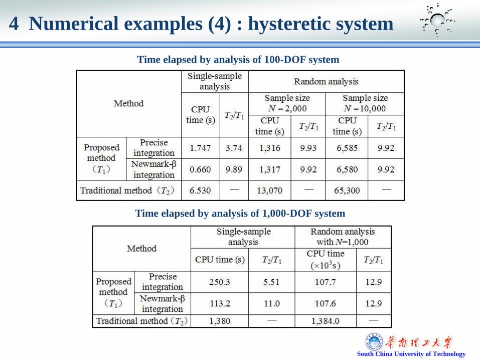
Time elapsed by analysis of 100-DOF system
Time elapsed by analysis of 1,000-DOF system
4 Numerical examples (4) : hysteretic system
South China University of Technology

1 Introduction
2 Explicit expressions of dynamic responses : linear systems
3 Explicit iteration MCS : nonlinear systems
4 Numerical examples
5 Concluding remarks
Contents
South China University of Technology

The non-stationary random vibration analysis of nonlinear systems with multiple degrees of freedom is one of the most difficult topics in the field of nonlinear random vibration. A new approach to this highly challenging problem is developed in the present study.
Two explicit iteration schemes based on precise integration and Newmark-β integration are proposed for fast MCS of non-stationary random vibration of nonlinear systems, including Duffing systems and hysteretic systems.
The coefficient matrices used for the solution need to be calculated just once and remain unchanged for different time steps and different samples. Therefore, the solution efficiency can be improved greatly, effectively breaking the bottleneck in MCS.
The proposed method provides a solid foundation for the application of random vibration analysis to large-scale nonlinear engineering problems.
5 Concluding Remarks
South China University of Technology

South China University of Technology