Explaining Cross-sectional Differences in

Market-to-Book Ratios

in the Pharmaceutical Industry

Philip Joos1

William E. Simon Graduate School of Business Administration

University of Rochester

Rochester, NY 14627

philjoos@simon.rochester.edu

February 25, 2002

1This paper is based on my dissertation completed at the Graduate School of Business of Stan-ford University. I thank my reading committee, Mary Barth, Peter Reiss and especially Bill Beaver(chair) for their helpful comments and suggestions. I appreciate the comments of seminar participantsat Columbia University, Duke University, Harvard University, MIT, the University of California atBerkeley, the University of Chicago, the University of Michigan, the University of Rochester, and theUniversity of Washington at Seattle. Finally, I thank my wife, Margot Baetens, for her help with thepharmaceutical data collection, as well as for explaining the medical terminology.

Abstract

This study examines how accounting information is valued in a research-intensive industry,

the pharmaceutical industry. Investors are often concerned that the conservative accounting

treatment of research and development (R&D) investments is causing a reporting bias, resulting

in accounting summary numbers being less value-relevant for research-intensive firms. The

paper examines how accounting return on equity (ROE) and R&D are valued for a sample

of research-intensive companies and relate the valuation coefficients to both economic and

accounting recognition determinants. The empirical results support the four hypotheses on the

effects of competitive structure, R&D success, and growth in R&D investments on the ROE

and R&D valuation coefficients.

1 Introduction.

This paper examines how accounting information is valued in a research-intensive industry, the

pharmaceutical industry. I consider economic context as well as the conservative accounting

treatment of research and development investments as the major determinants of cross-sectional

differences in market-to-book ratios. Investors are often concerned that the conservative ac-

counting treatment of research and development (R&D) investments is causing a reporting bias,

resulting in accounting numbers being less value-relevant for research-intensive firms (Lev and

Sougiannis 1996). I explicitly address the valuation of earnings, book value of equity, and R&D

investments in an accounting based valuation model, and relate differences in valuation coeffi-

cients to competitive structure and accounting conservatism proxies. Prior literature (such as

Amir and Lev (1996)) focuses on the statistical significance of proxies for intangibles by linearly

adding these to a valuation model that includes book value of equity and earnings.1 In this

paper, I argue that nonacounting variables related to competitive structure do not enter the

valuation model as separate terms, but rather affect the coefficients on the accounting variables

in the valuation equation. The challenge is to formulate a theoretical valuation model in which

one can show the nonlinear effects of the economic primitives on the valuation of the accounting

variables. A similar approach is taken by Biddle et al. (2001), who relate the difference between

market value and book value of equity to current residual income, and examine the convexity

(nonlinearity) of the the slope coefficient on residual income.

I focus on a particular industry - the pharmaceutical industry - for four reasons. First, I

want to overcome several shortcomings of broad cross-sectional studies. In particular, compet-

itive structure variables (such as barriers-to-entry, concentration, and market share) contain

much measurement error when calculated on a large variety of firms in different industries.

By focusing on a single industry, I hope to derive less noisy competitive structure variables.

Second, I want to study an industry with high levels and large enough cross-sectional variation

in market-to-book ratios. Third, I have two important contextual supplemental disclosures

available over a long period to compute competitive proxies: drug information from the Food

and Drug Administration (FDA) and patent information from the U.S. Patent Office. Finally,

1Amir and Lev (1996) use market penetration, number of subscribers, total population (POPS) as nonfinan-cial measures for intangible capital.

1

relatively large R&D investments are an important feature of the pharmaceutical industry.

However, U.S. accounting standards require firms to expense these investments rather than to

capitalize them. R&D recognition and the valuation consequences for earnings, book value and

R&D expenses are important research issues.

Consistent with Palepu et al. (2000) and reasons explained later in the paper, I deflate the

valuation equation by book value of equity. The resulting valuation equation puts the market-

to-book ratio as a linear function of book return on equity (ROE) and R&D expenses deflated

by book value (RDBV ). The R&D term is the distinctive feature of the model when compared

to other residual income valuation specifications in the recent accounting literature. I focus

on R&D because it is a key element in the production function of pharmaceutical companies

and because it is the major source of accounting conservatism in this industry. R&D enters

the valuation equation through an economic durability parameter that represents the degree of

success in R&D investments, in other words, the economic depreciation of R&D capital.

In the empirical design, I use proxies for growth in R&D investments, abnormal profitabil-

ity persistence and economic depreciation of R&D capital. I will refer to these as value driver

proxies. Two of the empirical measures capture aspects of the competitive structure of the

drug industry: firm type (pioneering versus generic drug firms) and a firm’s overall therapeutic

market share. The two competition proxies are expected to affect abnormal profitability persis-

tence, and therefore the valuation multiples on ROE and RDBV . The proxy for depreciation

of R&D capital is based on patent information. The number of patents granted to a firm is an

output-oriented measure of innovation, in contrast with the R&D expenditures that are input

oriented. Firms that are more successful in conducting R&D will have more patents per dollar

of invested R&D than firms that are less successful. The patent variable affects the economic

depreciation rate of R&D capital since successful R&D is expected to generate relatively more

future benefits (e.g., more revenues or higher cost-efficiency) than unsuccessful R&D. As a

consequence, the patent variable also affects R&D reporting bias in ROE. Finally, I have two

R&D growth proxies, one shortterm and one medium term growth variable.

There are four hypotheses in this paper. Two hypotheses relate to the effect of compet-

2

itive structure on the valuation coefficients of ROE and R&D, one relates to the valuation

effect of differential patent output per dollar of R&D, and the last hypothesis relates to R&D

growth effects on the valuation model. I predict that pioneering drug firms (versus generic drug

manufacturers) and firms with higher overall therapeutic market shares have higher valuation

multiples on ROE and R&D. I also predict that firms with a higher number of patents per

R&D dollar have a higher valuation coefficient on R&D. Finally, growth in R&D investments

combined with conservative accounting (the fully expensing of R&D) affect earnings and book

value of equity.2 I predict that higher growth in R&D investments results in higher valuation

coefficients on ROE and R&D. However, the last prediction depends on whether the level of

growth exceeds a specific threshold discussed later in the paper.

I test the four hypotheses on a sample of 35 drug manufacturers that operate in the phar-

maceutical preparation industry over the period 1975-1998. I also include information on their

wholly owned subsidiaries. The pooled cross-sectional time series sample has 15 generic and 20

pioneering parent drug firms. I match data obtained from the FDA and the U.S. Patent Office

with financial information. The regression model explaining differences in the market-to-book

ratio includes an intercept, ROE and scaled R&D as explanatory variables. The effect of the

competitive structure, patent and growth variables on the coefficients in the valuation equa-

tion is studied by defining dummy variables for the value driver proxies that interact with the

intercept, ROE and R&D variable. As a result, the three valuation coefficients can vary with

the level of the four value driver proxies.

Not only do I find that R&D should be included as a separate term in the valuation model

for research intensive firms, but also that competitive structure, R&D success and growth in

R&D investments affect the valuation multiples of ROE and R&D in predicted ways. I also

show that accounting loss firms, representing 11% of the sample, have much lower valuation

multiples on ROE and R&D than profit firms, suggesting a lower value relevance of both ROE

and R&D for these firms.

Section 2 explains some industry specific institutional terminology and describes the drug

2Chapter 17 in Penman (2001) illustrates the effect of investment growth on earnings, book value of equity,market-to-book ratio, price-earnings ratio under conservative, neutral and liberal accounting.

3

development and patent process. The next section derives a valuation model. Section 4 develops

the hypotheses. Section 5 describes the variables used in the empirical part of the study. Section

6 presents the empirical regression equations and empirical tests. Section 7 presents the data

to estimate the valuation model. Section 8 reports the regression results for the pooled sample.

Section 9 presents a summary and conclusions.

2 Pharmaceutical Industry.

2.1 The Drug Development Process.

Pharmaceutical manufacturers fall into two main categories: pioneering and generic drug firms

(Scott Morton 1998). I discuss several aspects of both types of manufacturers, and in particular

elements that describe the competition between and among these firms.

Pioneering drug firms undertake R&D to discover new drugs and bring them to market

under a brand name. Examples of pioneering drug firms are Abbott, Alza, Merck, and Pfizer.

The entire process of R&D, production, and quality control is regulated and monitored by

FDA. A pioneering firm must have an approved New Drug Application (NDA) to sell a new

product. Pharmaceutical R&D is composed of fairly standardized steps (PhRMA 1999, 27):

discovery, preclinincal tests, investigational new drug (IND) submission to FDA, three clinical

trials, NDA submission, and postmarketing testing. On average it took 14.9 years for drugs

approved between 1990 and 1996 to be discovered, tested and approved. The R&D investments

made in this long period are on average allocated as follows: 40% for preclinical activities, 30%

for clinical trials, and 20% for IND/NDA approvals, manufacturing and quality control. The

Boston Consulting Group estimated the pre-tax cost of developing a drug introduced in 1990

to be 500 million dollars, including the cost of research failures as well as interest costs over the

entire R&D period. Dimasi et al. (1995) estimate that on average only 3 out of 10 drugs are

able to recoup their R&D investments from their sales.

The large time lag and the magnitude of R&D investments coupled with GAAP required

expensing of R&D makes R&D the single most important determinant of MTB in the phar-

maceutical industry. I present a formal model of this in appendix B.

4

The second category contains generic drug manufacturers. A generic drug firm is an

“imitator” firm that submits an Abbreviated New Drug Applications (ANDA) to FDA. The

ANDA demonstrates that the generic drug is “bioequivalent” to the original branded drug

(manufactured by a pioneering drug firm). Alpharma, Mylan and Teva are examples of generic

drug manufacturers. Cimetidine is an example of a generic copy of Tagamet, an anti-ulcer

drug pioneered by Smithkline in 1977. Several generic firms introduced Cimetidine starting

from 1994 (e.g., Mylan in 1994, Teva and Zenith in 1995), after the patent protecting Tagamet

expired. Although manufacturing a generic drug and filing an ANDA is much less costly than

discovering and developing a new drug, entry costs are nevertheless significant for a generic

firm (facing price competition and high sunk costs) (Scott Morton 1999).3 The ANDA process

takes on average about 18 months from first submission of the application to final granting of

permission (Scott Morton 1998). A generic firm can enter a therapeutic market when a patent

protecting a pioneering drug expires. Typically, a patent expires after a drug has been on the

market for 12 years (Grabowski and Vernon 1994).4 The price of a generic drug is on average

between 40% and 60% lower than the original pioneering drug. As a result, the market share of

the pioneering drug significantly shrinks in the post-expiration period. A way for a pioneering

drug firm to deter entry and to keep a high market share even after patent expiration is to build

up brand loyalty. That is, a pioneering firm heavily promotes its products (visits to physicians

and pharmacists, advertising in medical journals, or direct mail) and hopes that physicians will

keep prescribing its products even after generic entry occurred (Hurwitz and Caves 1988).

I develop two value driver proxies from FDA data. One variable distinguishes generic firms

3Market entry by generics was relatively limited prior to the 1984 Drug Price Competition and PatentTerm Restoration Act (Hatch-Waxman Act) because of costly FDA requirements that had to be met by thegeneric products. That is, generic drugs often would have to duplicate many of the pioneer’s tests to gainmarket approval after patent expiration. The act facilitated the entry of generic drugs after patent expirationby requiring only an “abbreviated” application procedure from the generic firm while it also restored part ofthe patent life lost during the premarket regulatory process of pioneering drug introductions (Grabowski andVernon 1992). In addition, FDA inspects the equipment the firm plans to use to manufacture the generic drug,and also inspects early batches of the drug. The Congressional Budget Office provides a detailed report on theeffects of increased competition from generic drugs on the prices and returns in the pharmaceutical industryafter the 1984 Act (CBO 1998).

4Before 1984, it took on average 3 years between the patent expiration date and generic entry with a 40%probability that generic entry occurs. After 1984, it took on average 1.2 months, with a 91% probability thatgeneric entry occurs (CBO 1998, 67). The next section discusses the patent issue in more detail.

5

from pioneering firms, and another focuses on a firm’s market share within its therapeutic

markets.

2.2 Patents.

R&D expenditures are an ex ante cost or input measure and are not in themselves intangible

assets. However, market-to-book reflects the market’s expected success of current and future

R&D expenditures. The key determinant of success for a pharmaceutical firm is its ability to

bring out a succession of new products that have a significant market impact. Performance in

the development of successful new products is the key to understanding sales, earnings persis-

tence and valuation. While patents are clearly only one possible measure of success in R&D,

NDAs, as well as sales and market shares are alternative measures of research output. However,

patents are early indicators of R&D success since patent applications are usually submitted early

in the innovation process. I relate the annual number of filed (and eventually granted) patents

to past R&D investments as an empirical proxy for economic depreciation of R&D capital.

3 Valuation Model.

In this section, I derive an expression for the market-to-book (MTB) ratio as a linear function

of book return on equity and R&D investments (scaled by book value of equity). The R&D

term enters the valuation model because of the reporting bias in earnings and book value of

equity due to the fully expensing of R&D under current GAAP as opposed to capitalizing

R&D investments and subsequently depreciating R&D capital. I formalize the reporting bias

in appendix B. I refer to appendix A for an overview of the definition of the variables and

parameters used in the paper.

Ohlson (1995) shows that the dividend discount model can be rewritten in terms of book

value and expected future abnormal earnings. I prefer the use of a scaled residual earnings

valuation model to an unscaled version for two reasons. First, book return on equity (ROE) is

a central valuation measure (Palepu et al. 2000).5 Second, there is a statistical basis for using

5I also estimate an unscaled valuation equation with book value and earnings as separate variables as a

6

ROE as valuation measure. In particular, abnormal return on equity under R&D capitalization

(CROEa) is more likely to be a stationary series than unscaled abnormal earnings adjusted for

R&D capitalization (CNIa), where CROEa is defined as CROE − r, and CNIa is equal to

NIt− r BVt−1 (see table A). Qi et al. (2000) provide empirical evidence on the nonstationarity

of unscaled abnormal earnings, and also show book value and abnormal earnings do not coin-

tegrate with market value.6 Similar to Bernard (1994), I express market value (MV ) scaled by

book value under R&D capitalization as a function of abnormal return on equity under R&D

capitalization (CROEa) and growth in book value of equity (CBV ):

MVt

CBVt

= 1 +∞∑

τ=1

1(1+r)τ Et[CROEa

t+τ

CBVt+τ−1

CBVt

] ,

= 1 +∞∑

τ=1

(1+k)τ−1

(1+r)τ Et[CROEat+τ ],

(1)

where k is the non-stochastic growth rate of book value of equity under R&D capitalization

(k = CBVt+1

CBVt−1), CROEa (= CROE−r) is the abnormal book return on equity after adjusting

for R&D capitalization, and r is the non-stochastic discount rate for future expected dividends.

Similar to Ohlson (1995), I transform the infinite sum in eq.(1) into an empirically mea-

surable expression by specifying a linear information dynamic for CROEa. Similar to Geroski

(1990) who models excess economic profits, I assume abnormal CROEa follows an AR(1) pro-

cess:

CROEat+1 = ωCROEa

t + εt+1 ,

CROEt+1 = (1− ω)r + ωCROEt + εt+1 ,(2)

where ε is an i.i.d. disturbance term with mean zero. In other words, eq.(2) formalizes the idea

that competition eventually drives all profit rates to a competitive level r. The speed of conver-

gence to r is reflected in ω. The above assumption does not incorporate an other information

parameter as in Ohlson (1995). The other information will enter the valuation framework in

another way, as I show below. Note that I make an explicit stochastic assumption on CROEa

sensitivity check. The conclusions are not qualitatively changed.6Alternatively, I could transform unscaled CNIa into a stationary series through some order of differenc-

ing. However, the necessary order of differentiation is unknown and could be quite high. O’Hanlon (1997)demonstrates in his appendix that the presence of explosive properties of unscaled abnormal earnings couldeven prevent the transformation of the abnormal earnings series into a stationary series through differencing. IfR&D is not the only source of biased accounting recognition of economic income, then the mean CROE coulddeviate positively from the cost of capital r and might cause unscaled CNIa to exhibit explosive properties.

7

and not on reported ROEa, since CROE is assumed to be closer to the conceptual economic

profitability rate than ROE. Modeling the dynamic of ROEa is more complicated since ROE

is affected by typical characteristics of the accounting model, such as conservatism or delayed

recognition (in particular, expensing of R&D).7 At this point, I note that the assumption in

eq.(2) is the most essential difference with the Ohlson (1995) model, which assumes a stochastic

relation on unscaled abnormal earnings.

The rate of convergence of CROE (ω) to the cost of capital (r) is hypothesized to be a func-

tion of elements such as market competition (within a therapeutic market), barriers-to-entry,

and relative cost efficiency compared to other firms (Mueller 1990). These elements are part of

other information available at time t beyond accounting information. In the empirical analysis,

I explicitly study the effect of other information on the persistence parameter (ω) and other

valuation parameters (see below).

Using assumption (2) on the stochastic process of CROEa, I rewrite valuation equation (1)

as follows:MVt

CBVt

= 1 +ω

(1 + r)− ω(1 + k)CROEa

t , (3)

where ω(1 + k) < 1 + r is assumed. Higher abnormal return on equity persistence, ω, results in

a higher valuation coefficient on CROEa.8 Since current GAAP does not allow capitalization

of R&D expenses, I write the above valuation relation in terms of observable BV and ROE

assuming the growth rate of book value of equity under R&D capitalization (CBV ) is equal to

the growth rate of R&D investments (i.e., k = g):

MVt

BVt

= 1− ω(1+r)−ω(1+g)

r + ω(1+r)−ω(1+g)

ROEt + (1+r)(1+g)(1−ω)λ((1+r)−ω(1+g))(1+g−λ)

RDt

BVt

= Λ0 + Λ1ROEt + Λ2RDt

BVt

,(4)

The above equation expresses the market-to-book ratio as a sum of one minus a term involving

the cost of capital (r) plus a term with reported ROE plus a term with scaled R&D (RDt

BVt).

7Van Breda (1981) suggests to treat accounting rates of return as the output from an accounting “filter”, theinput to which are economic events. He shows that it is easier to understand the dynamics of the input processthan to understand the filtered output.

8In unreported analyses, I find empirical evidence supporting the AR(1) assumption of CROEa.

8

Since the dependent variable and both ROE and RDt

BVtare observable, the above equation can

be estimated.

I make several predictions on the effects of three key parameters (ω, g, and λ) on the

valuation coefficients Λ0, Λ1 and Λ2. I summarize the partial derivatives in the table below,

where R = 1 + r and G = 1 + g:

Parameter Intercept (Λ0) ROE (Λ1) RDBV (Λ2)

ω ∂Λ0

∂ω= −R(R−1)

(R−ωG)2∂Λ1

∂ω= R

(R−ωG)2∂Λ2

∂ω= RG(G−R)λ

(R−ωG)2(G−λ)

λ ∂Λ0

∂λ= 0 ∂Λ1

∂λ= 0 ∂Λ2

∂λ= RG2(1−ω)

(R−ωG)(G−λ)2

g ∂Λ0

∂G= −ω2(R−1)

(R−ωG)2∂Λ1

∂G= ω2

(R−ωG)2∂Λ2

∂G= Rλ(1−ω)[ωG2−Rλ]

(R−ωG)2(G−λ)2

I briefly discuss the effects of the three parameters ω, λ and g on the valuation coefficients Λ0,

Λ1 and Λ2 .

First, higher CROEa persistence (ω) results in a lower intercept, a higher valuation coeffi-

cient on ROE and an effect on the R&D coefficient that is positive when g > r and negative

when g < r, ceteris paribus. Written in mathematical notation: ∂Λ0

∂ω< 0, ∂Λ1

∂ω> 0 and

sign(∂Λ2

∂ω) = sign(g − r). Thus, when a firm experiences lower competition in its therapeutic

drug markets and therefore has a higher ω, its current level of ROE will have a higher valuation

multiple. From inspecting the partial derivatives, one notices that growth in R&D investments

determines the magnitude of the ω effect on the valuation multiples: higher growth increases

the effect of ω on both the ROE and R&D valuation multiple.

Second, Λ2 is the only coefficient that depends on λ, the durability of R&D capital. Higher

R&D durability resulting from more successful R&D investments shows up in a higher valuation

coefficient on RDBV , ceteris paribus (∂Λ2

∂λ> 0).

Third, higher growth in R&D (g) increases the valuation coefficient on ROE, and reduces

the intercept (Λ0), ceteris paribus: ∂Λ0

∂G< 0, ∂Λ1

∂G> 0. The growth effect on the R&D valuation

multiple depends on the sign of ωG2 − Rλ, or whether or not G >√

Rλω

. If a firm’s R&D

growth G is above the√

Rλω

threshold, then growth has a positive effect on the R&D multiple.

For example, a firm with a cost of capital of 10%, abnormal profitability persistence of 0.7, and

9

R&D durability of 0.9 has a cutoff value of 1.189. So, if the firm’s annual growth rate falls below

18.9%, then an increase in growth will have a negative effect on the R&D valuation multiple,

as long as the firm’s growth rate remains below 18.9%. I will discuss the above predictions in

more detail in the hypotheses section.

To summarize, I propose an accounting-based valuation model in which growth, R&D eco-

nomic durability, and profitability persistence affect the valuation of book return on equity and

R&D investments in a nonlinear fashion.

4 Hypotheses.

This section discusses testable hypotheses based on the valuation model in (4). The predictions

in the hypotheses are based on the partial derivatives of the valuation coefficients Λ0, Λ1 and

Λ2 with respect to ω, λ and g (see previous section). The first two hypotheses make predictions

on the effect of competition (ω) on the valuation coefficients. The third hypothesis focuses

on the economic duration parameter λ in the RDBV valuation coefficient. Finally, the fourth

hypothesis states a prediction on the effect of R&D growth on the coefficients in the valuation

model. I do not formulate a hypothesis on r, the cost of capital, but assume r is the same

across firms.

The first two hypotheses relate to the ω parameter in the valuation model. Firms with

more persistent abnormal profitability (CROEa) - a higher ω - will have a higher valuation

coefficient on ROE and lower intercept, assuming ω is uncorrelated with g, r, and λ. The effect

of ω on the RDBV valuation coefficient is expected to be positive if the firm has a growth

rate greater than its cost of capital, i.e., g > r. Abnormal profitability is negatively related

to competition. High competition within a specific therapeutic market (e.g., cardiovascular

drugs) could quickly drive profit rates to a longterm competitive level. Consistent with the

IO literature, I view competition as a primary determinant of ω. Effects of competition on g

and λ are less clear. Competition in a pharmaceutical market takes three forms: among brand

name drugs, between brand name drugs and generic substitutes, and among generic versions

of the same drug. The first hypothesis focuses on the distinction between generic firms and

10

pioneering drug firms. As explained in section 2.1, generic entry in a therapeutic market occurs

when patents of a pioneering drug expire, and when expected future payoffs are high enough

to make generic entry profitable. Grabowski and Vernon (1994) report an average decline of

a pioneering drug’s revenue of 30%, 21%, and 12% respectively in the first three years after

generic entry. Generic versions of a drug are sold on average 40% cheaper than the original

pioneering drug at retail prices when 1 to 10 generic firms enter a market, and 60% cheaper

when more than 10 generic firms sell copies of a given pioneering drug (CBO 1998, 33). Overall,

generic firms are more likely to experience higher immediate competition than pioneering drug

firms because they cannot use entry barriers such as patents. For example, 12 generic versions

for Tagamet (a pioneering anti-ulcer drug marketed by Smithkline since 1977) were introduced

between May 1994 and February 1997 after the patent on Tagamet expired in May 1994. The

hypothesis below is derived from the table with partial derivatives in section 3.

Hypothesis 1: Generic firms have less abnormal profitability persistence ω than pioneering

firms. As a result of a lower persistence, the valuation coefficient on ROE (Λ1) in eq.(4)

will be lower and the intercept (Λ0) will be higher for generic firms compared to those

valuation coefficients of pioneering drug firms, ceteris paribus. Pioneering firms will have

a higher valuation multiple on R&D (Λ2) relative to generic firms, only if their growth

rate of R&D investments exceeds their cost of capital.

Rather than simply differentiating between generic and pioneering drug firms, the next hy-

pothesis focuses on another dimension of competitive structure, in particular market share.

Pioneering drugs often compete within the same therapeutic market with other pioneering and

generic drugs. Pioneering drug competition happens among NDAs, where the first marketed

drug is called breakthrough drug and the others me-too drugs. Me-too drugs are new molec-

ular entities (pioneering drugs) that are similar, but not identical, in molecular structure and

mechanism to the original or breakthrough new molecular entities.9 At first glance, the overall

9Consider the example of Tagamet, a pioneering anti-ulcer drug that was introduced in 1977 by Smithkline(therapeutic code 0874 in appendix D). Tagamet was the first drug to relieve ulcers by blocking the histamine2 (H2) receptors in the lining of the stomach from stimulating acid production by the parietal cells. Suchtreatment is generally superior to antacids, which only neutralize stomach acid. Seven years after Tagametbecame available, Glaxo-Wellcome introduced Zantac, which became the largest-selling drug in the world. Twoadditional H2 antagonists, Pepcid and Axid, were marketed by Merck (1986) resp. Eli Lilly (1988). Four slightlydifferent drugs using the same therapeutic mechanism (blocking the H2 receptor) were all patentable, and the

11

pharmaceutical industry does not appear to be highly concentrated, but when narrower ther-

apeutic markets are considered, concentration (or competition) varies widely. A firm’s market

share reflects the results of competitive forces. Market share is a measure for a firm’s market

power within a therapeutic market and is affected by quality differences, patent positions (for

pioneering firms), scale-related efficiencies (Allen and Hagin 1989), and price discrimination

(through brand name loyalty). Higher market power leads to higher persistence of economic

profitability. Therefore, market share directly affects the ω parameter in the valuation model.

Hypothesis 2: Firms with a large market share will have higher abnormal profitability per-

sistence ω than firms with small market shares. As a result, Λ1 in eq.(4) will be higher

and Λ0 will be lower for firms with higher market shares compared to firms with lower

market shares, ceteris paribus. The R&D valuation multiple will only be higher for firms

with larger market shares if the growth rate of these firms is greater than their cost of

capital, ceteris paribus.

The third hypothesis is related to the R&D process, in particular to elements affecting λ.

The coefficient on RDBV in eq.(4) might vary across pharmaceutical firms due to cross-sectional

differences in λ, even though all firms could have high degrees of R&D intensity (RDBV ). As

explained before, an essential activity in the industry is the generation of R&D knowledge. The

value of the knowledge investments is reflected in the durability parameter λ. Firms that are

more effective in generating knowledge will have higher values for λ. As explained in section

2.2, an important output measure of knowledge is a firm’s patent activity. More successful

R&D should be valued more by the capital market than less successful R&D. Patent intensity

measures R&D success by relating patents to previous R&D investment. The hypothesis below

is derived from the table with partial derivatives in section 3.

Hypothesis 3: Firms with a higher number of patents per dollar invested in R&D will have

a higher economic durability of R&D capital (λ) and hence a higher coefficient on scaled

R&D (Λ2) in eq.(4) than firms with less patents per dollar R&D, ceteris paribus.

Finally, the fourth hypothesis addresses growth in R&D expense, i.e. the g parameter. The

growth parameter affects the three valuation coefficients in eq.(4). The current level of ROE

breakthrough drug had only six years of market exclusivity before being challenged by a competitor (CBO 1998,19).

12

will have a higher valuation coefficient for high growth firms compared to low growth firms. Lev

et al. (1999) address the relation between R&D growth and ROE in their table 3. Although

they find that high R&D growth firms tend to have high market-to-book ratios, they do not

make specific predictions on the ROE valuation coefficient as in this study. The g parameter

also affects the RDBV valuation coefficient (Λ2) in a non-linear way. The effect of growth

on the R&D valuation multiple is only positive if the following growth condition is satisfied:

G >√

Rλω

. I explained this condition in more detail in section 3.

Hypothesis 4: Firms with a higher growth rate in R&D expense (g) will have a higher val-

uation coefficient on current ROE (Λ1) and on scaled R&D (Λ2), but a lower intercept

(Λ0), ceteris paribus. The prediction on the R&D multiple only holds when the growth

condition G >√

Rλω

is satisfied, and is reversed otherwise.

5 Variables.

I use two sets of variables in this study: the financial variables ROE and RDBV being valued

in the valuation model, and the value driver proxies affecting the valuation coefficients on ROE

and RDBV . All the variables are measured at a firm level, where a firm is defined as the set

of a parent and its majority owned subsidiaries. I provide a more detailed discussion on this

issue in section 7.1. Appendix A lists all variables used in this paper.

The first set of variables is related to the financial variables in the valuation model and

are calculated from the Compustat database (see section 7). The dependent variable is the

market-to-book ratio, defined as the ratio of a firm’s market value at the end of the fiscal year

(Compustat item199 × item25) to its book value of common equity (item60). The return on

equity (ROE) is defined as the ratio of current year income before extraordinary items (item18)

to the previous year book value of equity (item60). Similar to Dechow et al. (1999), I eliminate

extraordinary items from the numerator of ROE because the nonrecurring components of net

income are not persistent over time. It is precisely the persistent (or recurring) components of

ROE that affect the valuation coefficient on ROE (Ohlson 1999). The last financial variable

is deflated R&D investments RDBV (item46 over item60).

13

In the second set of variables, I develop proxies for the parameters ω, λ and g in eq.(4). The

value driver proxies do not enter the regression model as simple linear conditioning variables, as

done in most of the the prior intangibles literature. Rather, my value driver proxies affect the

coefficients on the intercept, ROE and R&D in the valuation model. In particular, I consider

four variables.

The first variable relates to hypothesis 1. DFIRM is a dummy variable that makes the

distinction between generic and pioneering drug manufacturers. In section 2.1, I described the

economic differences between the two types of firms. Often, pioneering drug firms also market

ANDAs, or have subsidiaries that are generic producers.10 I classify a firm i as “pioneering” if

the majority of the drugs it sells in a specific year t are pioneering drugs (NDAs):

DFIRMit =

1 if FIRMit = #NDAit

#NDAit + #ANDAit> 0.5 (pioneering)

0 if FIRMit = #NDAit

#NDAit + #ANDAit≤ 0.5 (generic)

(5)

That is, for each sample firm-year observation I calculate the total number of the firm’s NDAs

that are still on the market versus the number of ANDAs (i.e. generic drugs). I cumulate the

new drugs introduced in a particular year across all years in a firm’s life to get a stock variable

on the drug portfolio at each point in time. I subtract the withdrawn or discontinued drugs

from the drug portfolio. If the proportion of NDAs in the drug portfolio is larger than the

proportion of ANDAs, then I classify the firm as a pioneer in that year. The DFIRM dummy

variable is equal to one if a firm is classified as a pioneering drug firm, and zero otherwise. By

using counts of drugs I assume that all drugs are of equal economic importance. Ideally, I would

base DFIRM on a breakdown of a firm’s total sales (or gross profits) into sales (gross profits)

from generic products and from pioneering drugs. However, this information is not available

to me. As a sensitivity test, I compare the company assignment by DFIRM to the business

description section in Moody’s Industrial Manual. Specifically, the assignment of each sample

firm in appendix C corresponds with the business description in the Moody’s Manual. The

assignment does not differ from the one I use.

10Although the same company rarely produces both a pioneering drug and its generic copy, some genericmanufacturers are subsidiaries of pioneering firms. Most generic subsidiaries do not produce copies of theirparent company’s drugs (CBO 1998, 34).

14

The second variable also relates to ω and measures a firm’s overall average market share in

its therapeutic markets. The previous proxy only distinguished between pioneering and generic

firms as a competition measure affecting ω. The current variable incorporates all sorts of compe-

tition within a therapeutic market. That is, between (pioneering) breakthrough drugs, generic

substitutes and me-too drugs. A firm’s market share reflects the results of that competition.

Ideally, I want to measure market share as a firm’s dollar amount of sales in a therapeutic

market divided by the total sales of all firms active in that market. Relating a firm’s total sales

number to the total sales of all sample firms does not correspond with the theoretical notion

underlying market share: a firm should be compared to its rivals in a particular therapeutic

market.11 I would need to have individual drug sales (a dollar amount) for the period 1975-1998

for all my sample firms and their subsidiaries. Individual drug sales data from IMS Health (a

large pharmaceutical data-collection firm) Drugstore and Hospital Audits were used by Taylor

(1999) and Scott Morton (1999) among others. However, it is not feasible to obtain a compre-

hensive dataset with yearly sales figures for all the drugs in my dataset. As an alternative, I

define the average market share of firm i in year t as follows:12

MSit =1

Jit

Jit∑j=1

(#NDAijt + #ANDAijt)∑Njt

i=1(#NDAijt + #ANDAijt), (6)

where #NDAijt (resp. #ANDAijt) is the stock of NDAs (ANDAs) of firm i in market j in

year t, Jit is the total number of therapeutic markets in which firm i is active in year t, and

Njt is the total number of firms active in market j in year t. The MS proxy is an average of

11For example, Genentech is a focused pioneering drug firm that concentrates its R&D on human growth hor-mone deficiencies (hGHD; code 1042 in appendix D). Genentech introduced its rDNA engineered drug Nutropinin 1993, 14 years after its scientists first cloned the human growth hormone. Genentech’s direct rivals and theirdrugs are: Tap Pharmaceuticals, a joint venture between Abbott and Takeda (Lupron, 1985), Lilly (Humatrope,1987), Pharmacia & Upjohn (Genotropin, 1987), Bio-Technology General (Bio-Tropin, 1995), and Ares-Serono(Saizen, 1997). Genentech’s ability to earn an abnormal profitability rate to sustain its persistence (ω) is directlyrelated to the competitive forces in the hGHD market, and not so much to the entire pharmaceutical industry.

12The definition assumes all drugs are of equal importance in terms of sales. Grabowski and Vernon (1994)provide evidence of a highly skewed distribution of sales which exists for new drug introductions. Peak sales ofthe top decile are several times that of the next ranked decile. Furthermore, mean sales are significantly greaterthan median sales. The distribution of individual drug sales clearly reflects the blockbuster drug influence, i.e.only 10% of all NDAs have an average (after tax) present value over their drug life cycle of 1 billion dollar.Seventy percent of the new drugs do not exceed the average present value of their R&D costs (200 milliondollar).

15

a firm’s market shares in a particular year across all therapeutic markets in which it operates.

The denominator in the above definition represents the total number of drugs in the same ther-

apeutic class, i.e. the population of drugs for that particular class. Similar to Scott Morton

(1999), I define therapeutic markets based on the National Drug Code (NDC) classification

provided by the FDA (see appendix D for an overview of the 117 therapeutic markets). The

same classification scheme is used in Mosby’s GenRx, an influential medical reference used by

physicians. For drugs without a therapeutic class in the NDC list, I use the Merck Index to

assign a therapeutic class. One drug can be used for several illnesses and can therefore be

classified in more than one class. The NDC classification is very detailed, and drugs within

each category can be considered as competitors. This feature is desirable for the purpose of this

study. There are several ways to define therapeutic markets, usually at a more aggregate level.

Egan et al. (1982) and Matraves (1999) provide a more detailed discussion. As a result of the

narrow market definitions, small firms could have large values on MS if they have a dominant

position in small niche markets. Large firms, on the other hand, could have small MS values

if they are only active in very large therapeutic markets with many other competitors. Notice

that MS is an indicator of a firm’s market power, and therefore directly affects ω (see hypoth-

esis 2): firms with a dominant market position are able to sustain a high level of abnormal

economic profitability and therefore have high market-to-book ratios.

The third variable relates to the R&D economic durability parameter λ in the patent hy-

pothesis (Hypothesis 3). Patent intensity, PAT , is measured as the ratio of the number of

patent applications at the US Patent Office in a particular year to the three-year backward

moving average R&D investment:

PATit =# Patent applications it

13

∑2τ=0 RDit−τ

. (7)

That is, patents are the result of past research efforts (here the most recent three years), and

are therefore deflated by average R&D investments. Notice that the numerator of PAT is a

count variable, and the denominator is a dollar amount. This type of deflation is common in

the patent literature, for example Ben-Zion (1984) deflates by book value of equity and Hall

et al. (1999) deflate by total assets. I use patent applications instead of patent grants in the

16

numerator, since the patent application date is a better indication of the time of innovation

than the issuance date (Hall et al. 1999). The ratio is a measure of the innovation and R&D

success of a firm. Only eventually granted patents appear in the US patent database. A patent

truncation bias at the end of the sample period occurs due to the lag between application and

grant.13 That is, in the final sample years not all the grants for patents applied for appear.

Similar to Hall et al. (1999), I adjust the patent count variable between 1993 and 1998 as

follows:

# Patent applications adjit =

# Patent applications it∑98−tτ=0 fiτ

93 < t < 98

where the numerator on the right hand side is the unadjusted number of patent applications of

firm i in year t, and fiτ is the firm-specific average proportion of patent applications granted

τ years after the application year t. The denominator of the adjustment formula represents

the firm’s historical cumulative frequency of patents granted τ years after application. Since

the cumulative frequency is close to one for τ = 6, the adjustment is only performed for the

final six sample years (1993-1998). For example, Merck has the following frequency fτ pattern:

7.97% for τ = 1 (i.e., the percentage of patent applications that are granted within the first

year of application), 59.14% for τ = 2, 23.56% for τ = 3, 6.39% for τ = 4, 1.6% for τ = 5, and

finally 0.47% for τ = 6. Thus, on average 99.13% of the patent applications are granted within

six years after application.

Malerba et al. (1997) give some caveats on the use of patent count data. First, not all

innovations are patented by firms. Secrecy, particularly in the case of process innovations, is

sometimes a more effective appropriation mechanism (Encaoua et al. 1998). However, in the

pharmaceutical industry, most pioneering firms file their patents early in the drug innovation

process (around the time they file an IND to FDA).Second, patents do not grant complete

monopoly power in the pharmaceutical industry (CBO 1998). The reason is that firms can

frequently discover and patent several different drugs that use the same basic mechanism to

treat an illness. That is the case for me-too drugs (see above).14 Third, patents cannot be

13The median firm-specific application-grant lag in the sample varies between 16 and 41 months.14For example, Alza mentions the following in its 1997 annual report: “Although a patent has a statutory

presumption of validity in the U.S., the issuance of a patent is not conclusive as to such validity or as to theenforceable scope of the claims of the patent. There can be no assurance that patents of Alza will not be

17

distinguished in terms of relevance without specific analyses on patent renewals or patent ci-

tations. Patents have an extremely skewed distribution of private patent values, meaning that

only a small fraction of patents has a high value (Hall et al. 1999). As a result, a simple patent

count is expected to be a noisy measure of a firm’s R&D success.

The fourth and last variable relates to the g parameter in hypothesis 4. I define R&D

investment growth, RDG, as the yearly growth in R&D expenses:

RDGit =RDit

RDit−1

− 1 , (8)

where RDit is firm i’s R&D expense in year t. The RDG variable is a short-term growth

measure, and might not fully be consistent with the constant g assumption in the valuation

model. I therefore define an alternative (annualized) R&D growth measure that spans a longer

time window:

LTRDGit = 3

√13

∑2τ=0 RDit−τ

13

∑5τ=3 RDit−τ

− 1 , (9)

where the numerator is the three year (moving) average of R&D investments in period [t−2, t],

and the denominator is the average R&D investment in period [t − 5, t − 3]. The expression

within the root is therefore a three year growth, and is annualized by taking the proper root.

6 Econometric Analysis.

In this section, I present the empirical specification of the ROE-based valuation model discussed

in section 3. A first empirical specification for the valuation model in eq.(4) is:

MTBt = α + βROEt + γRDBVt + εt (10)

where MTB is the market-to-book ratio, RDBV is the ratio of R&D to BV (or scaled R&D),

and ε is a stochastic disturbance assumed to be I.I.D. I could estimate the above equation in

successfully challenged in the future. In some cases, third parties have initiated reexamination by the Patentand Trademark Office of patents issued to Alza, and have opposed Alza patents in other jurisdictions. Thevalidity and enforceability of Alza patents after their issuance have also been challenged in litigation. If theoutcome of such litigation is adverse to Alza, third parties may then be able to use the invention covered by thepatent, in some cases without payment.”

18

different ways by making different assumptions on the variance-covariance matrix of the distur-

bance term. A firm-specific estimation of the above regression model suffers from inefficiency

in the valuation parameters due to the short time-series since there are only between 8 and

24 observations per firm available. To make better use of the cross-sectional variation in the

dataset, I pool the firm data into one cross-section time series sample and study the effects of

ω, λ and g on that pooled sample (see below).

One characteristic of the pharmaceutical industry is the high frequency of negative earnings.

In the final sample, 11.5% of the firm-year observations represent accounting losses, and 22 out

of 35 firms had at least one year with negative earnings. Hayn (1995), Collins et al. (1999),

and Leibowitz (1999) report differences in valuation coefficients between positive and negative

earnings.15 Similar to these studies, I differentiate between firms with positive and negative

earnings, and allow the intercept (α), ROE coefficient (β), and RDBV coefficient (γ) to vary

across positive and negative earnings firms through the indicator variable DNEGt, which is

equal to 1 if a firm has negative earnings in year t, and 0 otherwise.

I study the effects of the four value driver proxies FIRM , MS, PAT and RDG (or,

LTRDG) on the valuation coefficients α, β and γ in eq.(10) by defining a dummy variable

for each value driver proxy, and allowing each valuation coefficient to vary with these dummies.

That results in 25 = 32 possible values on the intercept, ROE and RDBV valuation coefficient,

since there are four different value driver (dummy) variables and the DNEG dummy :

MTBt = α0(1−DNEGt) +∑4

i=1 αiDUMMYit × (1−DNEGt)

+α5DNEGt +∑4

i=1 αi+5DUMMYit ×DNEGt

+β0(1−DNEGt)×ROEt +∑4

i=1 βiDUMMYit × (1−DNEGt)×ROEt

+β5DNEGt ×ROEt +∑4

i=1 βi+5DUMMYit ×DNEGt ×ROEt

+γ0(1−DNEGt)×RDBVt +∑4

i=1 γiDUMMYit × (1−DNEGt)×RDBVt

+γ5DNEGt ×RDBVt +∑4

i=1 γi+5DUMMYit ×DNEGt ×RDBVt + εt ,

(11)

15In particular, Leibowitz (1999) suggests three reasons for differences between positive and negative ROEsand their relation with the market-to-book ratio. First, negative earnings could result from conservative account-ing, making the relation between market-to-book and negative ROE significantly negative. Second, negativeearnings as a result of negative transitory items that do not represent cash flows (e.g., changes in accountingmethods) make the relation between market-to-book and ROE negative. Finally, negative earnings as a resultof negative transitory items that do represent cash flows (e.g., adverse litigation outcome) have no significanteffect on the relation between ROE and market-to-book.

19

where DNEGt is the sign of earnings dummy variable, DUMMY1 (FIRM -dummy) is equal to

1 if a firm is a pioneering drug manufacturer, and 0 otherwise, DUMMY2 (MS-dummy) is equal

to 1 if a firm has a market share in the upper half of the sample, and 0 otherwise, DUMMY3

(PAT -dummy) is equal to 1 if a firm has a number of patents per dollar of average past R&D

that exceeds the median sample value, and 0 otherwise, and DUMMY4 (RDG-based) is equal

to 1 if a firm has a growth in R&D that exceeds median sample growth, and 0 otherwise.

I prefer to interact dichotomized versions of the value driver proxies with ROE and RDBV

over the originally continuous value driver proxies, since the interaction effects are predicted

to be nonlinear (see the table with partial derivatives on page 9). One derives the valuation

coefficients for a specific firm by adding the estimated α’s (β and γ respectively) multiplied by

the values on DUMMYit and DNEGit that apply to that firm for year t. For example, the

coefficient on ROE for a pioneering drug manufacturing with positive earnings, large market

share, high relative patent output, and low growth is: β0 + β1 + β2 + β3. The coefficient on

ROE for a generic drug manufacturer with an accounting loss, small market share, no patents

and large growth is: β5 + β9. As indicated earlier, there are 32 possible summing schemes.

The specification of regression equation (11) with the five dummy variables and the inter-

action terms allows me to study the effect of each value driver proxy, discussed in section 5,

on the valuation coefficients while controlling for all value driver proxies simultaneously. The

β0 to β4 coefficients are the ROE valuation coefficients for the positive ROE firms, and the

β5 to β9 coefficients are valuation coefficients on ROE for the negative earnings firms. The

effect of MS on the ROE coefficient after controlling for the sign of earnings, type of drug firm,

patent success, and growth, is reflected in β2 (for positive earnings firms) and β7 (for negative

earnings firms). For example, a positive β2 indicates an upward effect on the ROE valuation

coefficient by having a larger market share (see hypothesis 2). Based on the findings in earlier

mentioned studies, the various possible sums of the ROE β’s for negative earnings firms , i.e.

sums consisting of elements from {β5, β6, β7, β8, β9} , is expected to be close to zero or nega-

tive. A sum close to zero is consistent with the abandonment option hypothesis discussed by

Hayn (1995), Burgstahler and Dichev (1997) and Barth et al. (1998). A significantly negative

sum would be consistent with the empirical findings of Burgstahler (1998) and Leibowitz (1999).

20

The empirical specification in eq.(11) also allows me to examine the difference in R&D val-

uation between positive and negative earnings firms, and the effects of the four value driver

proxies on the R&D valuation coefficient. The γ coefficients of positive earnings firms (γ0 to

γ4) only differ from the γ coefficients of negative earnings firms if the former type of firm has

different values on λ, ω, g and r than the latter. For example, I refer to the above studies that

found lower earnings persistence for loss firms than for positive earnings firms. Lower earnings

persistence reduces ω in eq.(4) and therefore reduces (increases) the coefficient on RDBV if

g < r (g > r), ceteris paribus.

I estimate the coefficients in equation (11) on a pooled time series - cross-section dataset of

pharmaceutical firms. I employ a multivariate outlier deletion rule to eliminate the 1% most

extreme observations on both tails of the DFFITS distribution (see Belsley et al. (1980) for

more details). The t-statistic on a coefficient indicates whether a value driver (FIRM , MS,

PAT or RDG) has a statistically significant effect on a valuation coefficient, i.e. the intercept,

ROE and RDBV coefficient respectively. In order to compare the estimation results to prior

studies, I also estimate the following four benchmark models on the pooled dataset:

Model 1 : MTBt = α + βROEt + εt

Model 2 : MTBt = α + βROEt + γRDBVt + εt

Model 3 : MTBt = α0(1−DNEGt) + α1DNEGt + β0(1−DNEGt)×ROEt

+β1DNEGt ×ROEt + εt

Model 4 : MTBt = α0(1−DNEGt) + α1DNEGt + β0(1−DNEGt)×ROEt

+β1DNEGt ×ROEt + γ0(1−DNEGt)×RDBVt

+γ1DNEGt ×RDBVt + εt

The first benchmark model simply specifies the market-to-book ratio as a linear function of

ROE. The second model adds a separate term for R&D to the equation, and is identical to

eq.(10). The third benchmark model is similar to the first model, but distinguishes between

positive and negative earnings firms. I allow positive earnings firms to have a different intercept

and slope coefficient on ROE from the coefficients of the negative earnings firms. Finally, the

fourth benchmark is similar to the second model, but allows the intercept, coefficient on ROE

and RDBV to differ between positive and negative earnings firms.

21

7 Sample and Descriptive Statistics.

7.1 Sample Selection and Data.

The sample consists of firms primarily active in the “Pharmaceutical Preparation” industry

(SIC 2834), i.e. firms controlled by the FDA. I do not include firms from other pharmaceutical

4-digit industries: “Medicinal Chemicals And Botanical Products” (SIC 2833), “In Vitro And In

Vivo Diagnostic Substances” (SIC 2834), “Biological Products, Except Diagnostic Substance”

(SIC 2836), since these are not the typical pioneering and generic drug firms. The first year

in the sample is 1975 since accounting rules for R&D were modified in 1975.16 Similar to Lei-

bowitz (1999), I eliminate firm-year observations with negative book values of equity (4.6% of

the original sample), since ROE for these firm-years cannot be interpreted in economic terms,

i.e., firms with losses and negative BV have a positive ROE. The final sample consists of 35

firms, listed in appendix C, and 620 firm-year observations.

The firm-year observations on MTB, ROE and RDBV are matched with the value driver

proxies described in section 5. I use Moody’s 1998 Industrial Manual, OTC Unlisted Man-

ual, OTC Industrial Manual, Bioscan (Febr 1999), and Securities Data Company’s Platinum

M&A 1999 database to determine a sample firm’s subsidiaries, ownership and acquisition date.

The Moody’s manual reports company name changes, important information for later name

matches. I finally track the parent and subsidiary names in the FDA and patent databases.

The computation of the FIRM and MS variables is based on data provided by FDA. In

particular, the Freedom of Information (FOI) Office of FDA provides comprehensive data on

drugs approved by the FDA, such as tradename, generic name, firm, FDA approval date, and

withdrawal date. However, the FOI CDROM has no information on therapeutic class. I collect

16In particular, in 1974 FASB published SFAS No.2 “Accounting for Research and Development Costs” tostandardize and simplify accounting practice by requiring all R&D costs be charged to expense when incurred.Before SFAS No.2, the lack of explicit rules resulted in a broad range of different procedures being adoptedfor reporting purposes. Also, before 1975 some firms that were extensively involved in R&D did not disclosespecific data regarding their R&D programs. R&D expenditures were often aggregated with other items on theincome statement. The firms that did specify the amount of R&D in their financial statements, adopted oneof the three following reporting alternatives. The majority included R&D expenditures as a separate line itemin the income statement. Some included it in a footnote, while others reported it elsewhere in the unauditedsections of the financial statements (Dukes 1974, 18-21).

22

therapeutic class information from FDA’s National Drug Code (NDC) list, available at the FDA

website. I match the FOI data with the therapeutic class based on tradename, generic name,

firm and approval date. I use the Merck Index to assign a therapeutic class to drugs that could

not be matched with the NDC list. I provide a list of therapeutic classes in appendix D. The

final (merged) dataset contains 9,254 drugs approved between 1950 and 1998. That number

includes all approved drugs, not only the number of drug approvals for the sample firms and

their subsidiaries (3,168 drugs).

For the computation of PAT , I use information from the U.S. Patents database of Com-

munity of Science, a comprehensive bibliographic patent database that contains more than 1.7

million patents issued since 1975 (the first sample year). I search the database on parent and

subsidiary name. I aggregate the patent application information at a firm-year level by adding

all patents of a parent and its wholly owned subsidiaries in each year. The final patent dataset

contains 41,834 patents for the 35 sample firms.

7.2 Descriptive Statistics.

7.2.1 Descriptive Statistics for the Pooled Sample.

Table 1 presents distributional features of the key Compustat variables in the study for the

pooled sample: MTB (market-to-book), ROE (reported return on equity), RDBV (R&D to

book value of equity ratio), RDG (shortterm growth in R&D), LTRDG (longterm growth in

R&D), and BV G (yearly growth in book value of equity). The distribution of ROE is skewed

to the left, since mean ROE is 4% lower than median ROE. The median market-to-book ratio

is 3.6, much larger than the overall median ratio of 1.13 for all Compustat firms (Beaver and

Ryan 2000). The distribution of MTB is skewed to the right. The median ratio of yearly R&D

investments to book value is 11.7% with an interquartile range of 10.6%. Often in the literature

on pharmaceuticals, advertisement is considered as an important intangible (Matraves 1999).

For the current sample, the median ratio of advertisement expenses to book value of equity

is 6% with an interquartile range of 9.4%. Thus, the magnitude of advertisement expenses is

almost half that of R&D, with a larger variance.

23

The majority of firms in the sample are pioneering firms, so median FIRM is larger than

0.5. Median market share is 5.2% with an interquartile range of 6.2%. Patents (PAT ) are

expressed in units of million dollars of R&D. Ninety percent of the observations are between 0

and 2.5 patents per million dollar spent on R&D, with a median of 0.25 patents. The short-

term R&D growth measure, RDG, is much more volatile than the longterm measure, LTRDG.

For example, the interquartile range of RDG is 20.5%, compared to 15.3% for LTRDG. This

finding is not surprising, given that LTRDG is based on three year averages. By inspecting

the difference between means and medians, the distribution of RDG is much more affected

by extreme values than the distribution of LTRDG. Finally, the distribution of the growth

rate of reported book value of equity, BV G, is very similar to the distribution of shortterm

growth in R&D, RDG. That finding supports the assumption in the valuation model and ROE

prediction model that k = g.

7.2.2 Descriptive Statistics by High and Low Value Driver Groups.

Table 2 contains medians of key variables calculated by “high” and “low” value driver groups.

That is, I group the sample firms into two subsamples based on DFIRM , MS, PAT and RDG

respectively. On the first line, I report the median for each high and low group, the difference

between the group medians, and on the second line, I report the interquartile range (Q3-Q1)

within each group and the Wilcoxon Z-score to test the significance of the difference in medians.

The Wilcoxon Z-score is normally distributed.

The firms classified as generic drug manufacturers have a median proportion of 7.9% of

pioneering drugs in their drug portfolio, whereas the pioneering firms have a median of 84.8%

of pioneering drugs in their portfolio. Generic firms (FIRM 6 0.5) represent 36% of the total

sample. Low MS firms have a median of 3.4% market share versus 7.6% in the high MS group.

The patent output variable (PAT ) shows a median of 7 patents per 100 million R&D in the low

PAT group versus 53 patents in the high PAT group. Finally, low growth firms have a median

growth of 8.1% versus 28.3% for the high growth firms. Next, I discuss table 2 sequentially by

each of the variables in the first column.

24

The market-to-book ratio is clearly different between generic and pioneering drug manu-

facturers, as expected: 3.29 for the former and 3.84 for the latter. Market share is also a

variable that strongly differentiates between low and high market-to-book ratios. Both PAT

and RDG are not able to discriminate between market-to-book ratios, since the difference in

median MTB between the high and low PAT and RDG group are not statistically significant.

The fact that low RDG and high RDG firms have almost identical market-to-book ratios is

rather surprising. One explanation for the low association between R&D growth and MTB is

that historical growth is a bad proxy for future growth opportunities, which are reflected in the

market-to-book ratio. Another explanation is that the degree of R&D reporting bias in BV

varies between the two growth portfolios, and thus differentially affects the denominator of the

MTB ratio. The bias explanation is based on eq.(B.4): reported BV is less understated for high

growth firms than for low growth firms. Since R&D reporting bias in BV is inversely related

with growth, a high MTB ratio for the low-growth portfolio might result from an understated

BV , whereas a high MTB ratio for the high growth portfolio might reflect the existence of

future growth opportunities .

As expected, both ω proxies, DFIRM and MS, are good discriminators for ROE. In par-

ticular, low values on DFIRM and MS correspond with lower values on ROE. Notice that

even the median level of ROE in the generic group and low MS group is still high, i.e. 16.4%.

The higher ROE level for pioneering drug firms compared to that of generic firms, is consistent

with their higher market-to-book ratios. That could indicate either that pioneering firms are

more profitable in an economic sense, or that the R&D reporting bias in ROE is positive for

pioneering firms. Since I expect economic depreciation of R&D capital (1−λ) to be lower for pi-

oneering drug firms than for generic firms (pioneering firms can profit more and longer from the

results of their investments in R&D capital resulting from patent positions, superior knowledge,

etc.), the latter explanation is highly plausible. Table 2 indeed shows a significantly higher PAT

value for pioneering firms compared to the value for generic firms. Also, I show in eq.(B.6) that

the sign and magnitude of R&D bias in ROE depends on the difference between R&D growth

and reported ROE. RDG is 14.4% for pioneers versus 20.2% for generics (see below for a dis-

cussion), and the reported ROE level is 21.3% for pioneers versus 16.3% for generics, indicating

an upward bias in ROE for pioneering firms, and downward bias in ROE for generic firms,

25

i.e., ROE reported by generic firms is lower than it would be under R&D capitalization. The

observation on the bias effect for the pioneering firms is consistent with claims by Taylor (1999)

and PhRMA (1999) that accounting profitability measures for pioneering drug firms are upward

biased. Finally, the level of ROE is almost identical in the low and high PAT and RDG groups.

Pioneering drug firms have a median RDBV of 0.146 compared to 0.089 for generic firms.

That is consistent with relatively higher R&D investments undertaken by pioneering firms in

their long drug development process. Since firms with smaller market shares are typically

generic firms, low MS firms also have lower RDBV values compared to high MS firms. Fi-

nally, RDBV is not different between high and low PAT and RDG groups.

Pioneering drug firms typically have high market shares, and generic firms typically have

small market shares, indicating MS and FIRM are highly positively correlated. Proof of the

high positive correlation is shown in the MS column of table 2: there is a significantly different

value in FIRM between the low MS and the high MS groups (0.20 versus 0.75).

The patent output per million dollar invested in R&D is reflcted in PAT . Since patents are

key to pioneering drug firms to protect their developed drugs from competitors for a number of

years, it is not surprising that pioneering firms have a significantly higher value on PAT than

generic firms: 0.25 versus 0.20. Generic firms mainly have process patents, while pioneering

firms have product patents. High MS firms also have significantly higher patent output than

low MS firms: 0.27 versus 0.16 patents per million R&D. That is not surprising given the high

correlation between FIRM and MS.

Finally, annual growth in R&D investments is reflected in RDG. As indicated above, pio-

neering firms have a significantly smaller growth in R&D investments than generic firms: RDG

for pioneers is 14.4% versus 20.2% for generics. The high R&D growth rate of generic man-

ufacturers is mainly attributed to the 1984 Hatch-Waxman Act that promoted the supply of

generic drugs. At the same time of the Hatch-Waxman Act, changes in the demand for drugs

- brought on by newer forms of health care delivery and financing - have influenced both the

frequency with which generic and pioneering drugs are prescribed and the prices paid for them.

26

I refer to paper 2 of the Congressional Budget Office study on competition in the pharmaceu-

tical industry for more details (CBO 1998). Not surprisingly, firms with lower market shares

(typically generic firms) have a higher growth in R&D than firms with higher market shares:

RDG is 17.2% for low MS firms versus 14.2% for high MS firms.

7.2.3 Correlation Analysis.

Table 3 presents descriptives on the bivariate correlation structure of the key variables.Assuming

no spurious correlation due to the common deflator (BV ), market-to-book ratios are highly cor-

related with ROE (42% Spearman corr.) and RDBV (30%). In other words, both ROE and

RDBV are highly value-relevant. From the four value driver proxies, only FIRM and MS

are correlated with MTB, ROE and RDBV . The high positive correlations between FIRM

and RDBV , and between MS and RDBV confirm the findings in table 2. That is, pioneering

firms are more research intensive and have larger market shares than generic firms.

MS is significantly positively correlated with FIRM , confirming the results in table 2.

The high correlation between FIRM and MS strengthens the approach I take to formulate

hypotheses 1 and 2. That is, both hypotheses focus on the effect of the competitive structure

on ω. I use FIRM and MS as proxies for the competitive structure, and therefore assume

their main effect is on the ω parameter in the valuation model, and not on g, r or λ. RDG is

significantly related with LTRDG (both are different proxies for R&D growth). PAT is weakly

positively associated with MS and FIRM , since patenting firms are usually pioneering drug

firms with larger market shares. Consistent with Scott Morton (1999), FIRM is negatively

related with growth in R&D: the Hatch-Waxman Act of 1984 made it easier for generic firms to

introduce their generic substitutes to the market place, and therefore resulted in faster growing

R&D investments for generic firms. Since generic firms typically have smaller market shares,

MS is negatively associated with R&D growth.

27

8 Regression results.

This section discusses the estimation results of the valuation equation (11). I also report and

discuss the estimation of the four benchmark regressions discussed on page 21. All models are

estimated on the pooled cross-sectional time-series dataset. The second to fifth column in table

4 contains the benchmark estimation results, while the last column in the table contains the

results for the key valuation model.

The first benchmark regression (model 1) with ROE as the only explanatory variable in

the valuation equation has very little explanatory power : the adjusted R2 is 0.1%. Once

scaled R&D is added to the valuation model, the R2 increases from 0.1% in model 1 to 49% in

model 2. The dramatic increase in R2 and the significance of the RDBV coefficient is evidence

that λ is not zero, i.e., economic durability of R&D capital. The highly significant coefficient

on RDBV supports the valuation specification that includes R&D as a separate term, and

therefore suggests a non-zero λ. Lev and Sougiannis (1999), among others, also find significant

valuation multiples on R&D expenses for R&D intensive firms. However, in the rest of this

section, I extend previous studies by explaining the determinants of cross-sectional differences

in the valuation multiples on both R&D and ROE.

Similar to model 1, the third benchmark model (model 3) only has ROE as explanatory

variable, but allows a different intercept and slope between positive and negative earnings firms.

Consistent with the findings of Leibowitz (1999) among others (see section 6), the ROE val-

uation coefficient is significantly positive for positive earnings firms, and significantly negative

for negative earnings firms. The significantly negative ROE coefficient for negative earnings

firms contradicts the predictions in the option-style valuation model of Burgstahler and Dichev

(1997): the coefficient on negative ROE should be small and insignificant, consistent with the

adaptation value hypothesis. However, if losses are generated by conservative accounting, such

as R&D accounting, and if they do not reflect economic losses, then the market can indeed

place a significantly negative valuation multiple on negative ROE (Leibowitz 1999).

The fourth benchmark model adds RDBV to model 3 and also distinguishes between pos-

itive and negative earnings firms. Interestingly, the slope coefficient on ROE is almost zero,

28

which is consistent with the abandonment option hypothesis. In contrast with model 3, model

4 controls for accounting conservatism by having RDBV as a separate term in the equation.

The R&D coefficient is significantly positive for both negative and positive earnings firms, al-

though much lower for negative earnings firms (7.53 versus 17.51 for positive earnings firms).

The lower RDBV coefficient for negative earnings firms is most likely related to the difference

in abnormal profitability persistence between positive and negative earnings firms. Consistent

with prior literature, unreported results show that negative earnings firms have much lower

abnormal profitability persistence (ω) than positive earnings firms. In section 3, I demonstrate

that the partial derivative of the R&D valuation multiple with respect to ω is positive when

g > r. Thus, lower ω values imply lower R&D valuation multiples. Finally, the change in

explanatory power by adding RDBV to model 3 is again enormous: the adjusted R2 increases

from 21% in model 3 to 56% in model 4.

The results for the key valuation model in this study are reported in the last column (“model

5”) of table 4. Overall, the explanatory power of the model that includes the value driver prox-

ies is higher than that of the benchmark models: adjusted R2 is 66% compared to 56% of model

4. I discuss the effects of each of the four value driver proxies separately.

First, I focus on the effect of abnormal profitability persistence (ω) on the valuation coef-

ficients. Both FIRM and MS measure ω, and they affect the valuation coefficients through

DUMMY1 and DUMMY2 respectively. Since both measures are highly correlated, I discuss

their joint effect on equation (11). Both hypothesis 1 and 2 are strongly supported by the regres-

sion results. As expected, pioneering drug firms with large market shares have a significantly

lower intercept (both coefficients on DUMMY1 and DUMMY2 are significantly negative) and

higher coefficient on ROE. That is a result of pioneering firms having more persistent abnormal

profitability than generic firms, since the latter experience more immediate competition when

they introduce a drug (see section 2.1 for details). However, for the negative earnings firms

(i.e., NI < 0) that represent 11% of the sample, both MS and FIRM effects on the intercept

and ROE coefficient compensate each other, resulting in a zero effect on the two valuation co-

efficients. The effects of FIRM and MS on the R&D valuation coefficient depend on whether

growth in R&D investments exceeds the cost of capital. The annual R&D growth rate for

29

pioneering firms is 14.4% (see table 2) and cost of capital estimates for these firms are reported

by Taylor (1999) to vary between 15.6 (American Home Products) and 19.07 (Syntex) with an

average of 16.7 in the period 1975-1991.17 That would indicate that g < r for pioneering firms

and, as a consequence, both FIRM and MS are expected to have a negative effect on RDBV .

Table 4 shows a negative - but insignificant - effect of FIRM and MS on the R&D valuation

coefficient.

Second, I discuss the effect of PAT on the RDBV valuation coefficient. The regression

results strongly support hypothesis 3 that predicts a positive effect of patent success on the

R&D valuation multiple. The coefficient on DUMMY3 (PAT ) is highly significant in the pre-

dicted direction. That is, firms with relatively more patents per dollar invested in R&D have a

significantly higher valuation multiple on R&D. Depending on the rate of success of the R&D

investments, firms will have higher or lower valuation multiples on R&D, after controlling for

competition (ω) and growth (g) effects. Thus, in addition to model 2 and model 4 in table 4

that include a separate R&D term, model 5 allows me to distinguish between the R&D coef-

ficients of firms with different rates of R&D success. There is no significant effect of PAT on

the R&D coefficient of negative earnings firms.

Third, the effect of growth in R&D investments on the valuation coefficients in equation (11)

is reflected in the coefficients on DUMMY4. As predicted by hypothesis 4, RDG negatively

affects the intercept and positively affects the coefficient on ROE in a statistically significant

way. That is, high growth firms have a higher valuation multiple on the current level of ROE.

Finally, the effect of growth on the R&D valuation multiple is predicted to be positive if the

R&D growth rate is larger than√

Rλω

, and negative otherwise. I refer to section 3 for more

details. Table 4 shows a coefficient on DUMMY4 (i.e., effect of RDG) for R&D that is not

significantly different from zero. The effect is slightly positive for positive earnings firms, and

negative for negative earnings firms. Prior literature (e.g., Hayn (1995)) documents lower per-

sistence of losses compared to profits, i.e. ωNI<0 < ωNI>0. As a result of a lower ω, loss firms

are expected to have a much higher pivot point√

Rλω

than profit firms. For example, loss firms

17Ibbotson’s Cost of Capital Quarterly 1999 Yearbook reports a median CAPM cost of capital of 15.5 for SIC2834, with an interquartile range of [Q1,Q3]=[12.2,18.9]. When the small size premium is added to the CAPMestimate, the median becomes 17.6 and [Q1,Q3]=[13.5,20.8].

30

with r = 0.18, λ = 0.7 and ω = 0.1 have√

Rλω

= 2.87, whereas profit firms with r = 0.16,

λ = 0.8 and ω = 0.7 have√

Rλω

= 1.15. Unreported analysis shows that the observed growth

rate of loss firms is 0.19 compared to 0.15 for profit firms. Taking the above pivot points, the

observed growth rate of 0.15 is exactly equal to the growth condition, whereas the observed

growth rate of 0.19 is much below the pivot value of 2.87. The effect of growth on the valuation

multiple of R&D is therefore predicted and found to be negative. The fact that the coefficient of

-4.29 for the loss firms is not statistically significant is probably related to the high variance in

annual growth for the sample loss firms ([Q1,Q3]=[0.01,0.42] compared to [0.12,0.18] for profit

firms).

I illustrate the valuation specification for four different types of companies: (1) pioneering

drug firms with a large market share, high patent output, low growth, and positive earnings,

(2) generic drug firms with a small market share, low patent output, high growth, and positive

earnings, (3) same as case 1 but with negative earnings, and (4) same as case 2 but with negative

earnings. The following regressions are obtained by multiplying the DUMMYi value with the

estimated respective coefficients reported in table 4 (model 5):

1) pioneer (NI > 0) : MTBt = −1.96 + 14.2 ROEt + 20.31 RDBVt

2) generic (NI > 0) : MTBt = 1.46 + 4.48 ROEt + 18.52 RDBVt

3) pioneer (NI < 0) : MTBt = 2.31 − 3.47 ROEt + 0.13 RDBVt

4) generic (NI < 0) : MTBt = 1.14 − 3.15 ROEt − 1.03 RDBVt

For example, the intercept value of -1.96 for the pioneering drug firms with positive earnings

is calculated from table 4 as 2.52 − 1.72 − 1.63 − 1.13 = −1.96. The intercept value of 1.46

for the generic firms with positive earnings is calculated as 2.52 − 1.06 = 1.46. Pioneering

drug manufacturers with positive earnings have a much higher ROE valuation multiple than

generic firms due to higher abnormal profitability persistence: the ROE coefficient is 14.2 for

pioneers versus 4.48 for generics. The slightly higher R&D valuation multiple for pioneering

firms is a result of a higher λ for these firms, measured by PAT (see table 2). The λ effect

dominates the ω effect (measured by FIRM and MS) on the R&D multiple: the coefficient

on DUMMY3 is 10.05 versus the sum of the coefficients of DUMMY1 and DUMMY2 of -7.47.

The coefficient on ROE becomes slightly negative for loss firms: -3.47 for pioneers and -3.15

31

for generics. The abandonment option hypothesis would predict a coefficient close to zero on

ROE. The negative valuation coefficient might be caused by conservative accounting meth-

ods used by negative earnings firms, that are not captured by the R&D term. Examples of

such conservative accounting methods are the immediate write-off of purchased R&D (i.e., a

negative special item in the year of the write-off), and accelerated depreciation of fixed assets.

Again, I emphasize that the loss firm-year observations only represent 11% of the total sam-

ple. The R&D multiple is almost zero for both types of firms when they incur accounting losses.

To summarize, all four valuation hypotheses are strongly supported by the regression re-

sults. Not only do I find that R&D should be included as a separate term in the valuation

model for research intensive firms, but the regression specification in equation (11) allows me

to simultaneously examine the nonlinear effects of competitive structure, R&D success and

growth in R&D investments on the valuation multiples of ROE and scaled R&D. Loss firms,

representing 11% of the sample, have much lower valuation multiples on ROE and R&D than

profit firms, indicating a smaller value relevance of ROE and R&D for negative earnings firms.

Finally, I estimated an undeflated valuation specification as a sensitivity check, and the results

remain unchanged.

9 Summary and Concluding Remarks.

This paper examines how accounting information is valued in a research-intensive industry,

the pharmaceutical industry. I consider both economic context and R&D reporting bias as

main sources of differences in the valuation of accounting information. Prior literature - and

especially the intangibles literature - has taken a different approach as to how accounting and

nonaccounting information is valued by the stock market. In particular, most prior studies in-

clude nonaccounting information (describing a firm’s economic context) as separate linear terms

in a valuation equation. I argue that economic context determines the valuation coefficients

of the accounting variables. Bowen and Shores (2000), Hand (2001) and Shortridge (2001) are

among the few studies that interact economic context variables with accounting variables for

a sample of research-intensive firms, but none of these studies provide a theoretical valuation

model to study these interaction effects. By using a theoretical model, I show that the interac-

32

tion effects are often highly nonlinear in nature.

The valuation model relates the market-to-book ratio to book return on equity (ROE) and

R&D investments deflated by book value of equity (RDBV ). Abnormal profitability persis-

tence (ω), economic depreciation of R&D capital (λ), and growth in R&D investments (g) are

the value drivers affecting the valuation coefficients of ROE and RDBV . I interact four proxies

for these value drivers with the intercept, ROE and RDBV in the final regression equation.

The four hypotheses on the effect of each of the value driver proxies are strongly supported by

the regression results. First, differentiating between two types of drug firms (FIRM) shows

that pioneering drug manufacturers have a higher coefficient on ROE and lower coefficient on

RDBV due to higher persistence in abnormal profitability. For the same reason, firms with

larger therapeutic market shares (MS) have a higher coefficient on ROE and lower coefficient

on RDBV . Third, firms with more patent per dollar R&D investment (PAT ) have a higher

valuation multiple on scaled R&D due to a lower economic depreciation of R&D capital. Fi-

nally, higher growth in R&D investments positively affects the ROE valuation coefficient, and

has no effect on the R&D multiple.

There are several limitations to this study. First, I derive a parsimonious valuation model

in which R&D is the only source of reporting bias. Other sources of accounting conservatism,

such as expensing of advertisement, are not considered. However, I argue that R&D is the

key production factor for the sample companies, and the immediate expensing of the R&D

investments most likely captures a large proportion of accounting conservatism sources for

pharmaceutical firms. Second, the findings are based on a small sample of pharmaceutical

firms, and might not be valid for a larger universe of Compustat firms. I suspect the conclusions

of the study might be valid for other research intensive firms. Third, there are other sources

of cross-sectional differences in the market-to-book ratio of pharmaceutical firms that are not

used in the empirical analysis of the study. For example, I do not consider the valuation effects

of strategic alliances between companies (Hagedoorn and Schakenraad 1994; Nixon 1996).18 I

18For example, in November 1997 Merck signed a 145 million dollar research collaboration agreement withBiogen to develop VLA-4 for asthma and inflammation. Another common alliance is when pharmaceuticalfirms have marketing agreements, where one firm markets a drug that is developed by the second firm in aspecific geographic region. For example, Glaxo Wellcome signed a marketing agreement with the Japanesedrug manufacturer Fujisawa in 1994 to sell Imuran in the U.S. Finally, drug firms often have agreements with

33

also do not consider the outcome of clinical trials as a success indicator of R&D (I only use

patents as an R&D output measure). Despite these limitations, I find strong support for the

hypotheses on the effects of the four value drivers on the valuation coefficients of ROE and

RDBV .

universities: drug firms finance research activities performed by academic laboratories to acquire familiaritywith basic knowledge in a particular field. In addition, these agreements are important sources for recruitingqualified scientists and researchers (Gambardella 1995).

34

References

Allen, R.F. and A.S. Hagin. 1989. “Scale Related Efficiencies as a (Minor) Source of the Profits-

Market Share Relationship.” The Review of Economics and Statistics 71 (3): 523–526 (August).

Amir, E. and B. Lev. 1996. “Value-Relevance of Nonfinancial Information: the Wireless Communi-

cations Industry.” Journal of Accounting and Economics 22 (1): 3–30 (December).

Barth, M.E., W.H. Beaver, and W. Landsman. 1998. “Relative Valuation Roles of Equity Book

Value and Net Income as Function of Financial Health.” Journal of Accounting and Economics

25 (1): 1–34.

Beaver, W.H. and S.G. Ryan. 2000. “Biases and Lags in Book Value and Their Effects on the Ability

of the Book-to-Market Ratio to Predict Book Return on Equity.” Journal of Accounting Research

38 (1): 127–148 (Spring).

Belsley, D., R. Kuh, and R. Welsch. 1980. Regression Diagnostics. New York: Wiley.

Ben-Zion, U. 1984. Pages 299–312 in The R&D and Investment Decision and its Relationship to the

Firm’s Market Value: Some Preliminary Results. Chicago: The University Press of Chicago.

Bernard, V.L. 1994, January. “Accounting-Based Valuation Methods, Determinants of Market-to-

Book Ratios, and Implications for Financial Statement Analysis.” Working paper, University of

Michigan.

Biddle, G., P. Chen, and G. Zhang. 2001, January. “When Capital Follows Profitability: Non-Linear

Residual Income Dynamics.” Working paper, Hong King University of Science and Technology.

Bowen, R.M. and D. Shores. 2000, March. “Economic Context and the Value Relevance of Accounting

Data.” Working paper, University of Washington.

Burgstahler, D. 1998. “Discussion of ”Combining Earnings and Book Value in Equity Valuation”.”

Contemporary Accounting Research 15 (3): 325–341 (October).

Burgstahler, D. and I. Dichev. 1997. “Earnings, Adaptation, and Equity Value.” Accounting Review

72 (2): 187–215 (April).

CBO. 1998. How Increased Competition from Generic Drugs Has Affected Prices and Returns in the

Pharmaceutical Industry. Congressional Budget Office, Washington: CBO.

Collins, D.W., M. Pincus, and H. Xie. 1999. “Equity Valuation and Negative Earnings: The Role of

Book Value of Equity.” Accounting Review 74 (1): 29–61 (January).

35

Dechow, P.M., A.P. Hutton, and R.G. Sloan. 1999. “An Empirical Assessment of the Residual

Income Valuation Model.” Journal of Accounting and Economics 26:1–34.

Dimasi, J.A., H.G. Grabowski, and J.M. Vernon. 1995. “R&D Costs, Innovative Output and Firm

Size in the Pharmaceutical Industry.” International Journal of the Economics of Business 2 (2):

201–219.

Dukes, R.E. 1974, May. “Market Evaluation of Accounting Information: A Cross Sectional Test of

Investor Response to Expensing Research and Development Expenditures.” Ph.D. diss., Stanford

University, Graduate School of Business.

Egan, J.W., H.N. Higinbotham, and J.F. Weston. 1982. Economics of the Pharmaceutical Industry.

New York: Praeger Publishers.

Encaoua, D., B.H. Hall, F. Laisney, and J. Mairesse. 1998, June. “The Economics and Econometrics

of Innovation: An Overview.” Working paper, ENSAE.

Gambardella, A. 1995. Science and Innovation: the US Pharmaceutical Industry During the 1980s.

U.K.: Cambridge University Press.

Geroski, P.A. 1990. In Mueller 1990, 15–34.

Goto, A. and K. Suzuki. 1989. “R&D Capital, Rate of Return on R&D Investment and Spillover

of R&D in Japanese Manufacturing Industries.” The Review of Economics and Statistics 71 (4):

555–564 (November).

Grabowski, H.G. and J.M. Vernon. 1992. “Brand Loyalty, Entry, and Price Competition in Phar-

maceuticals after the 1984 Drug Act.” Journal of Law & Economics 35 (October): 331–350.

. 1994. “Returns on R&D on New Drug Introductions in the 1980s.” Journal of Health

Economics 13:383–406.

Hagedoorn, J. and J. Schakenraad. 1994. “The Effect of Strategic Technology Alliances on Company

Performances.” Strategic Management Journal 15:291–309.

Hall, B.H., A. Jaffe, and M. Trajtenberg. 1999, June. “Market Value and Patent Citations: A First

Look.” Working paper, NBER.

Hand, J.R.M. 2001, December. “The Market Valuation of Biotechnology Firms and Biotechnology

R&D.” Working paper, UNC Chapel Hill.

Hayn, C. 1995. “The information Content of Losses.” Journal of Accounting and Economics 20:125–

153.

36

Hirschey, M. 1982. “Intangible Capital Aspects of Advertizing and R&D Expenditures.” The Journal

of Industrial Economics XXX (4): 375–390 (June).

Hurwitz, M.A. and R.E. Caves. 1988. “Persuasion or Information? Promotion and the Shares of

Brand Name and Generic Pharmaceuticals.” Journal of Law & Economics 31 (October): 299–320.

Leibowitz, M.A. 1999. “Market-to-Book Ratios and Positive and Negative Returns on Equity.” The

Journal of Financial Statement Analysis Winter:21–30.

Lev, B. and T. Sougiannis. 1996. “The Capitalization, Amortization, and Value-Relevance of R&D.”

Journal of Accounting and Economics 21:107–138.

. 1999. “Penetrating the Book-to-Market Black Box: The R&D Effect.” Journal of Business

Finance & Accounting 26 (3): 419–449 (May).

Lev, B., B. Sarath, and T. Sougiannis. 1999, May. “R&D-Related Reporting Biases and Their

Consequences.” Working paper, New York University.

Malerba, F., L. Orsenigo, and P. Peretto. 1997. “Persistence of Innovative Activities, Sectoral

Patterns of Innovation and International Technological Specialization.” International Journal of

Industrial Organization 15:801–826.

Matraves, K. 1999. “Market Structure, R&D and Advertising in the Pharmaceutical Industry.” The

Journal of Industrial Economics 47 (2): 169–194 (June).

Mueller, D.C. 1990. The Dynamics of Company Profits: An International Comparison. U.K.:

Cambridge University Press.

Nixon, B. 1996. “Research and Development Alliances and Accounting.” R&D Management 26 (2):

169–175.

O’Hanlon, J. 1997. “The Time Series Properties of the Components of Clean Surplus Earnings: UK

Evidence.” Journal of Business Finance and Accounting 23 (2): 159–189 (March).

Ohlson, J.A. 1995. “Earnings, Book Values, and Dividends in Security Valuation.” Contemporary

Accounting Research 11 (2): 661–687.

1999. “On Transitory Earnings.” Review of Accounting Studies 4, no. 3 (forthcoming).

Palepu, K.G., V.L. Bernard, and P.M. Healy. 2000. Business Analysis and Valuation Using Financial

Statements. Cincinnati: South-Western College Publishing.

Penman, S.H. 2001. Financial Statement Analysis and Security Valuation. New York: McGraw-Hill.

PhRMA. 1999. Pharmaceutical Industry Profile 1999. Pharmaceutical Research and Manufacturers

of America, Washington: PhRMA.

37

Qi, D.D., Y.W. Wu, and B. Xiang. 2000. “Stationarity and Cointegration Tests of the Ohlson

Model.” Journal of Accounting, Auditing and Finance 15 (2): 141–160 (Spring).

Scott Morton, F.M. 1998, September. “Barriers to Entry, Brand Advertising, and Generic Entry in

the U.S. Pharmaceutical Industry.” Working paper, University of Chicago.

1999. “Entry Decisions in the Generic Pharmaceutical Industry.” RAND Journal of Eco-

nomics 30 (3): 421–440 (Autumn).

Shortridge, R.T. 2001, June. “Market Valuation of Successful Versus Non-Successful R&D Efforts

in the Pharmaceutical Industry.” Working paper, Ball State University.

Taylor, C.T. 1999. “The Cash Recovery Method of Calculating Profitability: An Application to

Pharmaceutical Firms.” Review of Industrial Organization 14:135–146.

Van Breda, M.F. 1981. The Prediction of Corporate Earnings. UMI Research Press.

Weiss, L.W. 1969. “Advertising, Profits, and Corporate Taxes.” The Review of Economics and

Statistics 51 (November): 421–430.

Zhang, X.-J. 2000. “Conservative Accounting and Equity Valuation.” Journal of Accounting and

Economics 29 (1): 125–149 (February).

38

Appendix AVariable Definitions.

Variables Definition

ANDA abbreviated new drug application (for generic drug)

BV reported book value of equity (Compustat item60)

BV G yearly growth rate of book value of equity

CBV book value of equity under R&D capitalization, see definition (B.1)

CNI net income under R&D capitalization, see definition (B.1)

CNIa abnormal net income under R&D capitalization, CNIt − r CBVt−1

CROE return on equity under R&D capitalization, see definition (B.5)

CROEa abnormal return on equity under R&D capitalization, CROE − r

DEPRD economic depreciation of R&D capital as defined in (B.3)

DFIRM dummy equal to one if FIRM > 0.5 and zero otherwise, see definition (5)

DNEG dummy equal to one if a firm has negative NI, and zero otherwise

FIRM proportion of NDAs in the drug portfolio as defined in (5)

LTRDG annualized three year growth rate of R&D as defined in (9)

MS aggregate therapeutic market share as defined in (6)

MTB market-to-book ratio, MVtBVt

NDA new drug application (for pioneering drug)

NI reported net income before extraordinary items (Compustat item237)

PAT number of patent scaled by average R&D expense of most recent three years

RD research and development expense (Compustat item46)

RDBV R&D intensity, R&D expense scaled by book value of equity

RDG yearly growth rate of R&D as defined in (8)

ROE reported book return on equity, NItBVt−1

ROEa abnormal book return on equity, ROE − r, where r is cost-of-capital

Parameters Definition

λ economic durability of R&D capital

Φ1 parameter describing R&D capitalization bias in reported earnings, see (B.4)

Φ2 parameter describing R&D capitalization bias in reported book value, see (B.4)

Λ0 intercept in valuation equation (4)

Λ1 coefficient on current reported ROE in valuation equation (4)

Λ2 coefficient on current RDBV in valuation equation (4)

ω AR(1) persistence parameter of CROEa

g firm-specific constant growth rate in R&D investments (G = 1 + g)

k growth rate in book value of equity under R&D capitalization

r cost-of-capital (R = 1 + r)

39

Appendix BR&D Capitalization Bias in Earnings and Equity Book Value.

Weiss (1969) was the first to provide a framework to analyze the reporting bias in return on equity

due to fully expensing of R&D. More recently, Lev et al. (1999) focus on this issue. Pharmaceutical

firms (both pioneering and generic firms) invest heavily in intangible R&D assets (or R&D capital).

As typically viewed by the literature, R&D capital represents the stock of knowledge a firm possesses

at a certain point in time, and is the most important production factor for a pharmaceutical firm.

The stock is accumulated through R&D efforts, and it depreciates and becomes obsolete due to such

conditions as development of superior techniques and the decline in appropriability of knowledge as

it diffuses (Goto and Suzuki 1989). Under current US GAAP, R&D investments are immediately

expensed. As a result, two accounting effects occur. First, earnings under current GAAP differ from

capitalized earnings (i.e. when intangible R&D capital would be capitalized and depreciated over its

expected economic life) because current R&D outlays are immediately expensed. Second, book value

of equity does not reflect investments in and depreciation of R&D capital.

I define the R&D capitalization effect on earnings and book value of equity as:

CNIt = NIt + RDt −DEPRDt,

CBVt = BVt +∞∑

τ=0

RDt−τ −∞∑

τ=0

DEPRDt−τ︸ ︷︷ ︸R&D capital

, (B.1)

where CNI is net income under R&D capitalization, NI is net income under current R&D GAAP,

RD is R&D expense, DEPRD is depreciation charge on R&D capital, CBV is book value of equity

under R&D capitalization, and BV is book value of equity under current GAAP. Eq.(B.1) holds for

any capitalization scheme. In particular, under current US GAAP, RDt is equal to DEPRt, that is

R&D investments are fully expensed. However, the R&D capitalization proposed in this study is one

that measures economic depreciation.

To operationalize (B.1), I make two assumptions. First, I assume R&D expenses follow a non-

stochastic exponential growth pattern with a constant growth rate g:

RDt+τ = (1 + g)τRDt (B.2)

Second, similar to Hirschey (1982), I assume yearly R&D investments have a constant economic

durability or retention rate λ. Assuming λ to be constant over time results in the following declining

40

balance depreciation formula:

DEPRDt = (1− λ)(1 + g)

1 + g − λRDt (B.3)

I implicitly assume λ < 1 + g and therefore do not allow negative growth rates of less than -1, since

0 6 λ < 1 + g. Firms conducting more successful R&D have a higher λ than firms with lower R&D

success.

Finally, substituting (B.2) and (B.3) in (B.1), the bias in reported NI and BV results in expression

(B.4):R&D related NI Bias = NIt − CNIt = − λg

1+g−λRDt = −Φ1RDt ,

R&D related BV Bias = BVt − CBVt = −λ(1+g)1+g−λRDt = −Φ2RDt .

(B.4)

where CNI is net income under R&D capitalization, NI is net income reported under current R&D

GAAP, RD is R&D expense, CBV is book value of equity under R&D capitalization, and BV is book

value of equity reported under current GAAP, g represents the time-constant R&D growth rate, and

λ is the time-constant economic durability of R&D (1 − λ represents the R&D depreciation rate). If

0 < λ 6 1, then a portion of the R&D expenditures in the current period will carry over to subsequent

periods and constitute an investment in intangible capital (or, R&D capital). On the other hand, if

λ = 0, then R&D expenditures only have an influence in the current period, and should be expensed

rather than capitalized. For example, unsuccessful R&D investments have little or no future benefits

for a firm. The above equations implicitly assume the growth rate in R&D is smaller than the R&D

depreciation rate, i.e., g < 1 − λ. Consistent with Zhang (2000), higher growth (g) increases the

net income bias, while it lowers the book value bias. When there is no growth, net income equals

earnings under R&D capitalization, but the equity book value bias remains different from zero (unless

λ becomes zero).

Next, I derive the bias in return on equity, ROE, since ROE will be one of the key explanatory

variables in the valuation model. Under R&D capitalization, the return on equity is defined as:

CROEt =CNIt

CBVt−1=

NIt + Φ1RDt

BVt−1 + Φ2RDt−1=

NIt

BVt−1+ Φ1

RDt

BVt−1

1 +Φ1

g

RDt

BVt−1

. (B.5)

If the capitalization corrected CROE does not contain any reporting bias, then CROE reflects a firm’s

internal rate of return. In section 3, I assume a stochastic process for CROE with an expected value

41

equal to the cost of capital. The R&D bias in reported ROE is expressed as:

R&D related ROE Bias = ROEt − CROEt =Φ2

RDt−1

BVt−1

1 + Φ2RDt−1

BVt−1

[ROEt − g] , (B.6)

where ROEt = NIt

BVt−1is book return on equity under current GAAP at time t. The above equation

provides insight into the sign and magnitude of the R&D bias in reported ROE. The bias is negative

(i.e., CROEt > ROEt or reported ROE understates economic profitability) if g > ROEt, and is

increasing in absolute value with increasing R&D intensity (RDt−1

BVt−1) and R&D economic durability (λ).

If ROEt equals g, then the R&D bias in ROE disappears. Consistent with Zhang (2000), in the case

of zero growth, reported ROE is always overstated (i.e., ROE exceeds capitalized CROE), and the

difference between ROE and CROE is positively related with R&D intensity and R&D durability.

For example, if R&D investments have no future benefits (λ = 0), then ROE = CROE when R&D

investments do not grow. Lev et al. (1999) provide a different approach in their proposition 1 to de-

scribe the sign and magnitude of the R&D reporting bias in ROE. In their model, the bias is positive

if ROE 6 g1+g/2 . The latter ROE condition leads to a similar prediction on the sign of the reporting

bias as in my eq.(B.6).

42

Appendix CSample Firms.

Obs Cusipa Permnob Tickera Company Namea Incorp. Datec Typed

1 002824 20482 ABT ABBOTT LABORATORIES 1900 P2 020813 65832 ALO ALPHARMA 1983 G3 022615 64856 AZA ALZA 1968 P4 026609 15667 AHP AMERICAN HOME PRODUCTS 1915 P5 110122 19393 BMY BRISTOL MYERS SQUIBB 1933 G6 17253C 64178 RXC CIRCA PHARMACEUTICALS 1978 G7 266354 10685 DRMD DURAMED PHARMACEUTICALS 1982 G8 284131 31799 ELN ELAN 1969 P9 312024 54819 FAUL FAULDING INC 1845 G10 345838 45241 FRX FOREST LABORATORIES 1956 G11 368710 38280 GNE GENENTECH 1976 P12 37733W 75064 GLX GLAXO WELLCOME 1873 P13 406369 10116 HDG HALSEY DRUG COMPANY 1935 G14 448924 68340 ICN ICN PHARMACEUTICALS 1960 G15 478160 22111 JNJ JOHNSON & JOHNSON 1887 P16 482740 46950 KV.A K V PHARMACEUTICAL 1941 G17 532457 50876 LLY LILLY (ELI) & CO 1876 P18 589331 22752 MRK MERCK & CO 1927 P19 552880 54798 MOGN MGI PHARMA 1979 P20 628530 69550 MYL MYLAN LABORATORIES 1970 G21 631728 80004 NSTK NASTECH PHARMACEUTICAL 1983 P22 670100 63263 NVO NOVO-NORDISK 1960 P23 717081 21936 PFE PFIZER 1900 P24 716932 75429 3PHFR PHARMACEUTICAL FORMULATIONS 1981 G25 717125 61138 PRX PHARMACEUTICAL RESOURCES 1978 G26 716941 82647 PNU PHARMACIA & UPJOHN 1886 P27 76242T 39570 RPR RHONE-POULENC RORER 1961 P28 806528 77075 SHR SCHERER (R P) 1972 G29 806605 25013 SGP SCHERING-PLOUGH 1935 P30 871616 37102 SYN SYNTEX CORP 1970 P31 881624 75652 TEVIY TEVA PHARMACEUTICAL INDUSTRIES 1985 G32 904801 78116 UMED UNIMED PHARMACEUTICALS 1962 P33 910571 78749 UG UNITED GUARDIAN 1942 P34 934488 24678 WLA WARNER-LAMBERT 1901 P35 989365 69155 ZENL ZENITH LABORATORIES 1968 G

a The cusip number, ticker, and company name are taken from the Compustat 1998 datafiles.b The permanent number in the CRSP database of 1999.c The incorporation date as mentioned in the history section of Moody’s Industrial Manual or Bioscan February1999 (American Health Consultants).d This column classifies the sample firms into generic (“G”) and pioneering (“P”) drug firms. The classificationis based on the level of FIRM (see definition 5): if the number of years DFIRM = 1 greater than the numberof years DFIRM = 0 over the sample period 1975-1998, then P appears in the column of this table, and viceversa.

43

Appendix DDefinition of Therapeutic Classes.

Obs FDA Classa Therapeutic Class Namea Firstb Pop.c Samp.c

1 0117 ANESTHETICS, LOCAL 1950 123 352 0118 ANESTHETICS, GENERAL 1951 27 113 0119 ANESTHESIA, ADJUNCTS TO/ANALEPTICS 1952 60 254 0281 ANTIDOTES, SPECIFIC 1953 54 145 0283 ANTIDOTES, GENERAL 1973 7 26 0346 PENICILLINS 1950 288 1127 0347 CEPHALOSPORINS 1965 208 988 0348 LINCOSAMIDES/MACROLIDES 1964 178 859 0349 POLYMYXINS 1957 12 810 0350 TETRACYCLINES 1950 150 6011 0351 CHLORAMPHENICOL/DERIVATIVES 1950 19 212 0352 AMINOGLYCOSIDES 1959 96 3113 0353 SULFONAMIDES/RELATED COMPOUNDS 1950 113 3514 0354 ANTISEPTICS,URINARY TRACT 1953 20 515 0355 ANTIBACTERIALS, MISCELLANEOUS 1950 173 8216 0356 ANTIMYCOBACTERIALS (INCL ANTI LEPROSY) 1950 54 717 0357 QUINOLONES/DERIVATIVES 1987 11 418 0358 ANTIFUNGALS 1950 150 6919 0388 ANTIVIRALS 1963 84 3920 0408 DEFICIENCY ANEMIAS 1951 36 1121 0409 ANTICOAGULANTS/THROMBOLYTICS 1950 78 2722 0410 BLOOD COMPONENTS/SUBSTITUTES 1952 20 423 0411 HEMOSTATICS 1952 14 824 0501 CARDIAC GLYCOSIDES 1954 9 725 0502 ANTIARRHYTHMICS 1950 167 4426 0503 ANTIANGINALS 1967 113 3727 0504 VASCULAR DISORDERS, CEREBRAL/PERIPHERAL 1953 23 828 0505 HYPOTENSION/SHOCK 1950 57 2729 0506 ANTIHYPERTENSIVES 1952 470 18130 0507 DIURETICS 1953 268 7031 0508 CORONARY VASODILATORS 1957 18 832 0509 RELAXANTS/STIMULANTS, URINARY TRACT 1974 19 433 0510 CALCIUM CHANNEL BLOCKERS 1985 61 1934 0511 CARBONIC ANHYDRASE INHIBITORS 1957 3 135 0512 BETA BLOCKERS 1981 40 1536 0513 ALPHA AGONISTS/ALPHA BLOCKERS 1974 11 437 0514 ACE INHIBITORS 1985 31 738 0600 CENTRAL NERVOUS SYSTEM 1979 2 139 0626 SEDATIVES/HYPNOTICS 1954 92 3940 0627 ANTIANXIETY 1956 171 6041 0628 ANTIPSYCHOTICS/ANTIMANICS 1954 162 4542 0630 ANTIDEPRESSANTS 1959 162 6343 0631 ANOREXIANTS/CNS STIMULANTS 1956 115 2544 0632 CNS, MISCELLANEOUS 1953 36 1745 0635 ANTIEMETICS 1954 19 846 0700 CONTRAST MEDIA/ RADIOPHARMACEUTICALS 1953 3 147 0789 DIAGNOSTICS, RADIOPAQUE AND NONRADIOACTIVE 1951 82 1248 0790 DIAGNOSTICS - RADIOPHARMACEUTICALS 1957 78 249 0792 DIAGNOSTICS, MISCELLANEOUS 1954 11 250 0874 DISORDERS, ACID/PEPTIC 1962 71 2851 0875 ANTIDIARRHEALS 1954 63 1952 0876 LAXATIVES 1956 14 153 0877 GASTROINTESTINAL, MISCELLANEOUS 1953 99 2754 0878 ANTISPASMODICS/ANTICHOLINERGICS 1950 22 955 0912 HYPERLIPIDEMIA 1964 34 1756 0913 VITAMINS/MINERALS 1950 117 3457 0914 NUTRITION, ENTERAL/PARENTERAL 1971 58 3758 0915 REPL/REGS OF ELECTROLYTES/WATER BALANCE 1951 281 7159 0916 CALCIUM METABOLISM 1953 20 7

44

Continued

Obs FDA Classa Therapeutic Class Namea Firstb Pop.c Samp.c

60 1032 ADRENAL CORTICOSTEROIDS 1951 308 8561 1033 ANDROGENS/ANABOLIC STEROIDS 1958 35 1162 1034 ESTROGENS/PROGESTINS 1951 131 5363 1035 ANTERIOR PITUITARY/HYPOTHALMIC FUNCTION 1955 36 964 1036 BLOOD GLUCOSE REGULATORS 1957 121 7365 1037 THYROID/ANTITHYROID 1956 13 566 1038 ANTIDIURETICS 1970 6 367 1039 RELAXANTS/STIMULANTS,UTERINE 1966 18 968 1040 CONTRACEPTIVES 1967 58 1669 1041 INFERTILITY 1954 12 270 1042 DRUGS USED IN DISORDERS OF GROWTH HORMON 1960 8 271 1180 VACCINES/ANTISERA 1987 2 172 1181 IMMUNOMODULATORS 1968 22 1173 1264 ANTISEPTICS/DISINFECTANTS 1950 28 874 1265 DERMATOLOGICS 1950 361 12875 1268 TOPICAL STEROIDS 1961 75 2776 1270 ACNE PRODUCTS 1973 15 577 1271 TOPICAL ANTI-INFECTIVES 1964 20 378 1272 ANORECTAL PRODUCTS 1957 3 279 1273 PERSONAL CARE PRODUCTS (VAGINAL) 1990 1 180 1274 DERMATITIS/ANTIPURETICS 1981 12 481 1371 EXTRAPYRAMIDAL MOVEMENT DISORDERS 1950 84 2482 1372 MYASTHENIA GRAVIS 1951 11 483 1373 SKELETAL MUSCLE HYPERACTIVITY 1951 180 4184 1374 ANTICONVULSANTS 1951 107 4985 1400 ONCOLYTICS 1992 1 186 1479 ANTINEOPLASTICS 1950 219 10687 1481 ANTIMETABOLITES 1968 3 188 1566 GLAUCOMA 1953 63 1589 1567 CYCLOPLEGICS/MYDRIATICS 1961 28 190 1568 OCULAR ANTI-INFECTIVE/ANTI-INFLAMMATORY 1950 203 3391 1569 OPHTHALMICS, MISCELLANEOUS 1953 35 192 1670 OTICS, TOPICAL 1953 28 793 1671 VERTIGO/MOTION SICKNESS/VOMITING 1951 261 7794 1700 RELIEF OF PAIN 1996 2 195 1720 ANALGESICS, GENERAL 1954 208 7396 1721 ANALGESICS-NARCOTIC 1950 204 6297 1722 ANALGESICS-NON-NARCOTIC 1979 24 698 1723 ANTIMIGRAINE/OTHER HEADACHES 1953 25 699 1724 ANTIARTHRITICS 1952 225 83100 1725 ANTIGOUT 1951 51 21101 1726 CENTRAL PAIN SYNDROMES 1978 11 4102 1727 NSAID 1959 109 35103 1728 ANTIPYRETICS 1989 4 3104 1860 ANTIPROTOZOALS 1953 48 15105 1862 ANTHELMINTICS 1953 21 11106 1863 SCABICIDES/PEDICULICIDES 1957 16 3107 1864 ANTIMALARIALS 1952 10 1108 1940 ANTIASTHMATICS/BRONCODILATORS 1951 257 89109 1941 NASAL DECONGESTANTS 1953 24 12110 1943 ANTITUSSIVES/EXPECTORANTS/MUCOLYTICS 1951 90 36111 1944 ANTIHISTAMINES 1950 148 50112 1945 COLD REMEDIES 1951 104 40113 1947 CORTICOSTEROIDS-INHALATION/NASAL 1982 8 6114 2087 UNCLASSIFIED 1950 78 29115 2095 PHARMACEUTICAL AIDS 1960 45 21116 2096 SURGICAL AIDS 1950 27 5117 2097 DENTAL PREPARATIONS 1954 30 7

total 9254 3168a FDA therapeutic class code and class name from National Drug Code Directory, available at:http://www.fda.gov/cder/drug.htm .b First drug in this class since start of the database (Jan 1950).c Pop. represents the total number of drugs in a particular class approved by the FDA between 1950 and 1998.Samp. is the drug count for the 35 sample firms. 45

Table 1:

Descriptive statistics for the pooled samplea

Variableb nobs Mean P5 Q1 Median Q3 P95

MTB 620 4.161 1.206 2.310 3.600 5.635 8.956ROE 615 0.159 −0.378 0.102 0.198 0.289 0.499RDBV 608 0.149 0.039 0.078 0.117 0.184 0.356FIRM 617 0.574 0.008 0.118 0.667 0.925 1.000MS 583 0.061 0.018 0.035 0.052 0.080 0.136PAT 536 0.568 0.000 0.078 0.250 0.618 2.458RDG 600 0.295 −0.190 0.083 0.155 0.288 0.963LTRDG 578 0.203 −0.058 0.116 0.163 0.269 0.580BV G 616 0.285 −0.244 0.040 0.135 0.260 0.976

a The table provides summary statistics on the distribution of the key variablesin the paper. The summary statistics are: nobs (number of sample observations),Mean (sample average), P5 (5th percentile), Q1 (1st quartile), Median (samplemedian), Q3 (3rd quartile), and P95 (95th percentile). The sample period covers1975-1998.b The variables are: MTB (market-to-book ratio), ROE (book return on equity),RDBV (the ratio of R&D to book value of equity), FIRM (proportion of NDAsin drug portfolio as defined in (5)), MS (market share as defined in (6)), PAT(number of patents to 3 year average R&D as defined in (7)), RDG (yearly growthrate of R&D investments as defined in (8)), LTRDG (annualized 3-year growthrate of R&D investments as defined in (9)), and BV G (yearly growth rate of bookvalue of equity, defined similar to RDG).

46

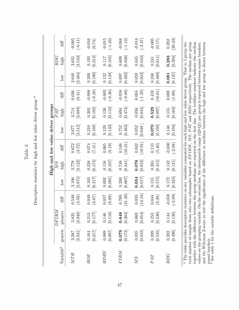
Tab

le2:

Des

crip

tive

stat

isti

csby

hig

han

dlo

wva

lue

driv

ergr

oup

a

Hig

han

dlo

wva

lue

dri

ver

grou

ps

DF

IR

MM

SP

AT

RD

GV

aria

bleb

gene

ric

pion

eer

diff

low

high

diff

low

high

diff

low

high

diff

MT

B3.

287

3.83

50.

549

3.10

63.

778

0.67

23.

677

3.71

40.

036

3.64

03.

635

-0.0

05[3

.341

][3

.948

](3

.50)

[3.8

75]

[3.1

22]

(3.7

2)[3

.512

][3

.688

](0

.41)

[3.4

84]

[3.5

43]

(-0.

11)

RO

E0.

164

0.21

30.

049

0.16

30.

238

0.07

40.

210

0.20

2-0

.008

0.20

90.

193

-0.0

16[0

.217

][0

.177

](3

.67)

[0.2

17]

[0.1

74]

(7.4

1)[0

.188

][0

.192

](-

0.28

)[0

.190

][0

.212

](0

.74)

RD

BV

0.08

90.

146

0.05

70.

092

0.15

80.

065

0.12

90.

126

-0.0

030.

132

0.11

7-0

.015

[0.0

87]

[0.1

16]

(8.0

9)[0

.091

][0

.107

](8

.19)

[0.1

33]

[0.1

10]

(-0.

36)

[0.1

28]

[0.1

05]

(-1.

33)

FIR

M0.

079

0.84

80.

769

0.20

00.

748

0.54

80.

752

0.69

4-0

.058

0.69

70.

609

-0.0

88[0

.173

][0

.304

](2

1.39

)[0

.667

][0

.341

](1

0.21

)[0

.483

][0

.474

](-

0.89

)[0

.492

][0

.838

](-

1.13

)

MS

0.03

50.

069

0.03

30.

034

0.07

60.

042

0.05

20.

056

0.00

40.

059

0.04

5-0

.014

[0.0

18]

[0.0

54]

(14.

18)

[0.0

17]

[0.0

52]

(18.

91)

[0.0

49]

[0.0

44]

(-1.

29)

[0.0

43]

[0.0

42]

(-3.

47)

PA

T0.

209

0.25

30.

044

0.15

50.

265

0.11

00.

070

0.52

90.

459

0.24

60.

241

-0.0

05[0

.545

][0

.536

](3

.28)

[0.5

75]

[0.4

15]

(5.4

0)[0

.193

][0

.897

](1

6.61

)[0

.488

][0

.611

](0

.17)

RD

G0.

202

0.14

4-0

.058

0.17

20.

142

-0.0

300.

146

0.15

50.

008

0.08

10.

283

0.20

2[0

.490

][0

.130

](-

2.89

)[0

.325

][0

.121

](-

2.08

)[0

.194

][0

.163

](1

.09)

[0.1

37]

[0.3

94]

(20.

33)

aT

heta

ble

prov

ides

desc

ript

ive

stat

isti

cson

key

vari

able

sco

mpu

ted

for

each

high

and

low

valu

edr

iver

grou

p.T

hat

is,I

grou

pth

eto

talnu

mbe

rof

sam

ple

firm

sin

totw

osu

bsam

ples

base

don

DF

IR

M,M

S,P

AT

and

RD

Gre

spec

tive

ly.

The

med

ian

per

grou

pto

geth

erw

ith

the

diffe

renc

ebe

twee

nth

egr

oup

med

ians

are

repo

rted

onth

efir

stlin

e.T

hebo

ldfa

cenu

mbe

rsin

dica

teth

em

edia

nva

lues

onth

egr

oupi

ngva

riab

le.

On

the

seco

ndlin

e,th

ein

terq

uart

ilera

nge

(Q3-

Q1)

per

grou

pis

repo

rted

betw

een

squa

rebr

acke

ts,

and

the

Wilc

oxon

Z-s

core

tote

stth

esi

gnifi

canc

eof

the

diffe

renc

ein

med

ians

betw

een

the

high

and

low

grou

pis

show

nbe

twee

nro

und

brac

kets

.b

See

tabl

e1

for

the

vari

able

defin

itio

ns.

47

Tab

le3:

Cor

rela

tion

mat

rix

for

the

pool

edsa

mple

ab

MT

BR

OE

RD

BV

FIR

MM

SP

AT

RD

GL

TR

DG

MT

B1

0.17

50.

331∗∗∗

0.17

70.

092

0.14

70.

016

0.03

9R

OE

0.42

0∗∗

1−

0.13

0−

0.01

20.

177

−0.

039

0.21

70.

065

RD

BV

0.30

1∗∗∗

0.04

51

0.24

8∗∗

0.16

5∗−

0.06

0−

0.00

80.

068

FIR

M0.

208∗

−0.

010

0.28

6∗∗∗

10.

500∗∗∗

0.14

3−

0.09

1−

0.13

4M

S0.

159

0.30

4∗0.

284∗∗

0.46

1∗∗∗

10.

009

−0.

070

−0.

026

PA

T0.

096

0.02

6−

0.07

80.

019

0.14

51

−0.

023

0.03

4R

DG

0.03

30.

080

−0.

017

−0.

061

−0.

084

−0.

016

10.

243

LT

RD

G−

0.01

1−

0.01

60.

036

−0.

152

−0.

052

−0.

036

0.29

9∗1

aT

heta

ble

prov

ides

Pea

rson

(upp

ertr

iang

le)

and

Spea

rman

(low

ertr

iang

le)

cros

s-se

ctio

nalco

rrel

atio

nco

effici

ents

amon

gth

eke

yva

riab

les

inth

epa

per.

The

corr

elat

ions

are

aver

ages

ofye

arly

cros

s-se

ctio

nalc

orre

lati

ons

over

the

sam

ple

peri

od19

75-1

998.

bT

heva

riab

les

inth

eta

ble

are:

MT

B(m

arke

t-to

-boo

kra

tio)

,R

OE

(boo

kre

turn

oneq

uity

),R

DB

V(r

atio

ofR

&D

tobo

okva

lue

ofeq

uity

),F

IR

M(p

ropo

rtio

nof

ND

As

indr

ugpo

rtfo

lioas

defin

edin

(5))

,M

S(m

arke

tsh

are

asde

fined

in(6

)),

PA

T(n

umbe

rof

pate

nts

to3

year

aver

age

R&

Das

defin

edin

(7))

,R

DG

(yea

rly

grow

thra

tein

R&

Das

defin

edin

(8))

,an

dfin

ally

,L

TR

DG

(ann

ualiz

ed3-

year

grow

thra

teof

R&

Das

defin

edin

(9))

.c

The

aste

risk

sre

pres

ent

the

sign

ifica

nce

ofa

corr

elat

ion

coeffi

cien

t.T

hesi

gnifi

canc

ele

velis

calc

ulat

edby

coun

ting

the

num

ber

ofye

arly

corr

elat

ions

that

have

oppo

site

sign

sth

anth

em

ajor

ity

ofco

rrel

atio

ns.

Thr

eeas

teri

sks

indi

cate

that

ther

ear

ele

ssth

an5%

year

lyco

rrel

atio

nsw

ith

oppo

site

sign

s.T

wo

(one

)as

teri

sk(s

)in

dica

teth

ere

are

betw

een

5%(1

0%)

and

10%

(15%

)ye

arly

corr

elat

ions

wit

hop

posi

tesi

gns.

48

Table 4:

Estimation results for the ROE-based valuation model a

Model 1 Model 2 Model 3 Model 4 Model 5Effectb NI > 0 NI < 0 NI > 0 NI < 0 NI > 0 NI < 0

Intercept 4.67 1.62 2.77 3.66 0.18 2.69 2.52 0.97(23.94) (9.70) (11.54) (7.06) (0.83) (6.03) (4.41) (1.16)

DUMMY1 (FIRM) − −1.72 4.70(−2.70) (3.59)

DUMMY2 (MS) − −1.63 −4.71(−2.66) −2.40)

DUMMY3 (PAT ) 0 −1.13 1.35(−2.26) (1.21)

DUMMY4 (RDG) − −1.06 0.17(−2.10) (0.14)

ROE 1.01 1.93 7.66 −5.62 7.34 −0.04 0.59 −1.07(1.88) (7.24) (11.53) (−5.85) (11.02) (−0.11) (0.37) (−0.77)

DUMMY1 (FIRM) + 9.13 1.90(3.88) (0.59)

DUMMY2 (MS) + 3.70 −4.88(1.53) (−1.35)

DUMMY3 (PAT ) 0 0.78 0.58(0.47) (0.21)

DUMMY4 (RDG) + 3.89 −2.08(2.50) (−0.59)

RDBV 16.94 17.51 7.53 17.73 3.26(22.94) (23.14) (5.00) (4.89) (8.89)

DUMMY1 (FIRM) − −4.78 −12.46(−1.29) (−3.00)

DUMMY2 (MS) − −2.69 11.40(−0.76) (1.47)

DUMMY3 (PAT ) + 10.05 −2.07(4.29) (−0.52)

DUMMY4 (RDG) ? 0.79 −4.29(0.33) (−0.79)

adjusted R2 0.1% 49% 21% 56% 66%# observations 603 591 603 591 527

a The ROE regression equations are estimated with OLS on the pooled sample, deleting the 1%most extreme observations at each side of the DFFIT distribution. The sample period covers1975-1998. The dependent variable in all regressions is the market-to-book ratio (MTB). Theindependent variables are indicated in the first column “effect”. Models 1 to 4 are benchmarkmodels (see page 21), while model 5 is the key valuation model in this study, i.e. eq.(11) on page19.b DUMMYi indicates a 0-1 variable and is based on one of the four value driver proxies: DFIRM ,MS, PAT and RDG. DUMMY1 (based on FIRM) is equal to 1 if a firm is a pioneering drugmanufacturer, and 0 otherwise; DUMMY2 (based on MS) is equal to 1 if a firm has a marketshare in the upper half of the sample (above the sample median), and 0 otherwise; DUMMY3

(based on PAT ) is equal to 1 if a firm has a number of patents per dollar of past R&D thatexceeds the median sample number, and 0 otherwise; and DUMMY4 (based on RDG) is equalto 1 if a firm has a growth in R&D that exceeds median sample growth, and 0 otherwise. Theeffect of the four dummy variables on the valuation coefficient of the intercept, ROE and RDBVis indicated by the + or − sign.

49