Explaining Credit Default Swap Spreads with Equity ...

Explaining Credit Default Swap Spreads with EquityVolatility and Jump Risks of Individual Firms∗

Benjamin Yibin Zhang†

Hao Zhou‡

Haibin Zhu§

First Draft: December 2004This Version: March 2005

(Preliminary and Incomplete)

Abstract

This paper explores the effects of firm-level volatility and jump risks on creditspreads in the credit default swap (CDS) market. We use a novel approach to identifythe realized jumps of individual equity from high frequency data. Our empirical resultssuggest that the volatility risk alone explains 50% of CDS spread variation, while thejump risk alone explains 23%. After controlling for ratings, macro-financial variables,and firms’ balance sheet information, we can explain 75% of the total variation. Thesefindings are in sharp contrast with the typical lower predictability and/or insignificantjump effect in the credit risk market. Moreover, firm volatility and jump risks showimportant nonlinear effect and strongly interact with the firm balance sheet informa-tion, which is consistent with the structural model implications and helps to explainthe so-called credit premium puzzle.

JEL Classification Numbers: G12, G13, C14.Keywords: Credit Default Swap; Credit Risk Pricing; Credit Premium Puzzle; Real-ized Volatility; Realized Jumps; High Frequency Data.

∗The views presented here are solely those of the authors and do not necessarily represent those of Moody’sKMV, the Federal Reserve Board, and the Bank of International Settlement. We thank George Tauchen forhelpful discussions.

†Moody’s KMV, New York. E-mail: [email protected].‡Federal Reserve Board, Washington D C. E-mail: [email protected].§Bank for International Settlements, Basel-4002, Switzerland. E-mail: [email protected].

1

1 Introduction

Structural-form approach on the pricing of credit risk can provide important economic in-

tuitions on what fundamental variables may help to explain the credit default spread. The

seminal work of Merton (1974) points to the importance of leverage ratio, asset volatility,

and risk-free rate in explaining the cross-section of default risk premia. Subsequent exten-

sions in literature include the stochastic risk-free interest rate process proposed by Longstaff

and Schwartz (1995); endogenously determined default boundaries by Leland (1994) and

Leland and Toft (1996); strategic defaults by Anderson et al (1996) and Mella-Barral and

Perraudin (1997); and the mean-reverting leverage ratio process in Collin-Dufresne and Gold-

stein (2001). These generalizations call for time-varing macro-financial variables and firm

specific accounting ratios as key determinants of the credit risk spreads. Further develop-

ment of the jump–diffusion default model along the lines of Zhou (2001) indicates that jump

intensity and volatility risks of firm value should have a strong impact on the credit spreads.

Despite the theoretical insights in understanding default risk, the empirical performance

of structural-form models is far from satisfactory. There has been recently a burgeoning

literature that points to the large discrepancy between the predictions of structural models

and the observed credit spreads, which is also known as the credit premium puzzle (Amato

and Remolona 2003). For instance, Huang and Huang (2003) calibrate a wide range of struc-

tural models to be consistent with the data on historical default and loss experience. They

show that in all models credit risk only explains a small fraction of the historically observed

corporate-treasury yield spreads. In particular, for investment grade bonds, structural mod-

els typically explain only 20-30% of observed spreads. Similarly, Collin-Dufresne et al (2001)

suggest that default risk factors have rather limited explanatory power on variation in credit

spreads, even after the liquidity consideration is taken into account. A recent study by Eom

et al (2004) finds that structural models do not always under-predict the credit spreads,

rather, those models produce large pricing errors for corporate bonds. Incorporating jump

risks has been helpful in explaining the level of credit spreads of investment-grade entities

with short maturities (cite?), however, historical skewness as a measure of jump risks is

usually insignificant statistically or having the wrong sign (cite?).

In this paper, we argue that the unsatisfactory performance of structural models may be

partially attributed to the fact that the impacts of volatility and jump risks are not treated

seriously in the previous studies. A prevalent practice is to use the average equity volatil-

2

ity within each rating category in calibration, which is subject to the “Jensen inequality”

problem if the true impact of volatility on credit spreads is not linear. Even when firm-

level equity volatility is used, historical volatility based on daily equity returns is often used,

which tends to smooth out the short term impact of volatility on credit spreads, especially the

jump risk impacts. More importantly, when jump effect is measured as historical skewness,

it may over-detect a model with asymmetric distribution but no jumps while under-detect a

model with symmetric jump distributions. The idea of emphasizing the links between equity

volatility or jump risks and credit spreads is not completely new. Campbell and Taksler

(2003) and Kassam (2003) observe that recent increases in corporate yields can be explained

by the upward trend in idiosyncratic equity volatility. This observation is consistent with

our findings in the this paper. Collin-Dufresne et al (2003) suggest that the jump risk alone

does not explain a significant proportion of the observed credit spreads of aggregate portfo-

lios. Instead, its impact on the contagion risk turns out to be associated with a much larger

risk premium. Cremers et al (2004a, 2004b) measure volatility and jump risk from prices of

equity index put options. They find that adding jumps and jump risk premia significantly

improve the fit between predicted credit spreads and the observed ones.1

Our contribution is to use high frequency return data of individual firms to decompose

the realized volatility into a continuous part RV(C) and a jump part RV(J). With stronger

assumptions, we are able to filter out the realized jumps and isolate the impacts associated

with jump intensity, jump volatility, and negative jumps. Therefore we can examine the

credit spreads more thoroughly with short term volatility and various jump risk measures,

in addition to the long-run historical volatility. Recently literature suggests that realized

volatility measures from high frequency data provides a more accurate measure of the short

term volatility (Andersen et al 2001, Barndorff-Nielsen 2002, and Meddahi 2002). Within

the realized volatility framework, the continuous and jump contributions can be separated by

comparing bi-power variation (from adjacent returns) and quadratic variation (from squared

returns) (see, Barndorff-Nielsen and Shephard 2004, Andersen at el 2004, and Tauchen and

Huang 2005, for the discussion of this methodology). Considering that jumps in financial

prices are usually rare and of large sizes, we further assume that (1) there is at most one jump

per day, and (2) jump size dominate daily return when it occurs. With filtered daily jumps,

we further estimate the jump intensity, jump mean (further decomposed into positive and

1In this paper, we refrain from using option-implied volatility and jump measures, because they arealready embedded with risk premia, which may have similar time-variation as credit spreads and need to beexplained by the same underlying risk measures as well.

3

negative parts), and jump volatility. We apply these new volatility and jump risk measures

in to explain the credit default swap spreads.

Our empirical results suggest that long-run historical volatility, short-run realized volatil-

ity (continuous), and various jump risk measures all have statistically significant and eco-

nomically large impacts on the credit spreads. The realized jump measures explain 23% of

total variations in credit spreads, while historical skewness and kurtosis measures on jump

risk only explain 3%. It is worth noting that volatility and jump risk alone predict 53%

of spreads variations. After controlling for ratings, macro-financial variables, and firms’

accounting information, the signs and significances of jump and volatility impacts remain

solid, and the R-square increases to 75%. These results are robust whether fixed effect

or random effect is taken into account. More importantly, both volatility and jump risk

measures show strong nonlinear effects, which suggests that the practice of using aggregate

volatility across board or within rating groups could either overestimated or underestimate

the true impact from individual firms. Finally, but not least, jump and volatility risk interact

prominently with rating groups and firm-specific financial variables. This evidence indicates

that the strong predictability of jump and volatility variables are not merely a statistical

phenomenon, rather, they reflect the financial market assessment of firms’ economic value

and financial health. In particular, the interaction between volatility & jump risks with the

quoted recovery rate suggests that credit default spreads have priced in the time-varying

recovery rates. These findings are consistent with a limited simulation exercise from stylized

structural models, and may help to resolve the so-called credit premium puzzle.

The remainder of the paper is organized as follows. Section 2 introduces the methodology

for disentangling volatility and jump risks with high frequency data. Section 3 gives a brief

discussion of data, and Section 4 examines the main empirical findings. A limited simulation

exercise is presented in Section 5, and Section 6 concludes.

2 Disentangling Jump and Volatility Risks

Equity volatility is central to asset pricing and risk management. Traditionally, researchers

have used the historical volatility measure, which are constructed from daily returns. A

daily return rt is defined as the first difference between the log closing prices on consecutive

trading days (Pt), that is

rt ≡ log Pt − log Pt−1 (1)

4

Historical volatility and historical skewness, which are defined as the variance and skewness

of the daily return series over a given time horizon, are considered as proxies for the volatility

and jump risk measures of the stochastic process of the underlying asset (for example, see

Campbell and Kassam 2003 and Cremers et al 2004a, 2004b).

In recent years, given the increased availability of high-frequency financial data, a number

of scholars, including Andersen and Bollerslev (1998), Anderson et al (2001, 2003), Barndorff-

Nielsen and Shephard (2002a, 2002b), and Meddahi (2002), have advocated the use of so-

called realized volatility measures by utilizing the information in the intra-day data for

measuring and forecasting volatilities. More recent work on bi-power variation measures,

which are developed in a series of papers by Barndorff-Nielsen and Shephard (2003a, 2003b,

2004), allows the use of high-frequency data to untangle realized volatility into continuous

and jump components, as in Andersen et al 2004 and Huang and Tauchen 2005. In this

paper, we rely on the stylized fact that jumps on financial markets are rare and of large

size, to explicitly estimate the jump intensity, jump variance, and jump mean (positive and

negative), and to assess more explicitly the impacts of volatility and jump risks on credit

spreads.

Let pt denote the time t logarithmic price of the asset, and it evolves in continuous time

as a jump diffusion process:

dpt = µtdt + σtdWt + κtdqt (2)

where µt and σt are the instantaneous drift and volatility, Wt is the standard Brownian

motion, dqt is jump process with intensity λt, and κ(t) refers to the size of the corresponding

(log) jumps.2 Time is measured in daily units and the intra-daily returns are defined as

follows:

rt,j ≡ pt,j·∆ − pt,(j−1)·∆ (3)

where rt,j refers to the jth within-day return on day t, and ∆ is the sampling frequency.3

Barndorff-Nielsen and Shephard (2003a, 2003b, 2004) propose two general measures to

the quadratic variation process, realized volatility and realized bipower variation, which

2A standard assumption is that κt observes a normal distribution.3That is, there are 1/∆ observations on every trading day. Typically the 5-minute frequency is used

because more frequent observations might be subject to distortion from market microstructure, which maydistort the properties of asset returns.

5

converge uniformly (as ∆ → 0) to different quantities of the jump-diffusion process,

RVt(∆) ≡1/∆∑j=1

r2t,j →

∫ t

t−1

σ2sds +

1/∆∑j=1

κ2t,j (4)

BVt(∆) ≡ π

2

1/∆∑j=2

|rt,j| · |rt,j−1| →∫ t

t−1

σ2sds (5)

Therefore the difference between realized volatility and bipower variation is zero when there

is no jump and strictly positive when there is a jump. A variety of jump detection techniques

are proposed and studied by Barndorff-Nielsen and Shephard (2004), Andersen et al (2004),

and Huang and Tauchen (2005). Here we adopt the ratio statistics used by Huang and

Tauchen (2005),

RJt(∆) ≡ RVt(∆) − BVt(∆)

BVt(∆)(6)

which converges to standard normal distribution, when appropriately scaled by its asymp-

totic variance estimate.4

This test has excellent size and power (Huang and Tauchen 2005), and tells us whether

there is a jump occurred during a particular day, and how much the jump-squared contri-

bution to the total realized volatility,∑1/∆

j=1 κ2t,j. To gain further insight, we assume that (1)

there is at most one jump per day and (2) jump size dominate return on jump days. This

methodology allows us to filter out the daily actual jumps as

Jt = sign(rt) ×√

RVt(∆) − BVt(∆) (7)

This method is consistent with the intuition that jumps on financial markets are rare and of

large sizes. Its effectiveness is still need to be justified in finite samples studies with realistic

empirical settings. This method enable us to estimate jump intensity λJ , jump mean µJ

(including signed jump means µ+J and µ−

J ), and jump standard deviation σJ , for a given

horizon (say one month or one year). Since jumps are rare, more accurate estimates of these

jump risk measures should be over the longer one-year horizon. Equipped with these new

technique, we are ready to reexamine the impact of jumps on credit spreads.

4See Appendix for implementation details and Huang and Tauchen (2005) for the finite sample perfor-mance of various competing jump detection statistics. We find that using the test level of 0.999 producesmost consistent result. We also use staggered returns in constructing the test statistics, to control for thepotential measurement error problem.

6

3 Data (to be revised)

Structural models provide an intuitive framework for identifying the determinants of credit

risk changes. A firm defaults whenever the firm value hits below an exogenously or en-

dogenously determined default boundary. Therefore the default probability of the firm is

determined by all factors that affect the firm value process, the risk-free interest rate, the

firm’s leverage ratio, default boundary and recovery rate.

In this section we first describe the data of credit spreads, which we obtain the premium

rates of credit default swaps (CDS) written on 307 reference entities. The theoretical de-

terminants of credit spreads are then divided into three major groups: (i) firm-level equity

volatility; (ii) firm’s balance sheet information; and (iii) macro-financial variables.

3.1 CDS spreads

We choose to use the CDS premium as a direct measure of credit spreads in this paper.

Credit default swaps are the most popular instrument in the rapidly-growing credit derivative

markets.5 A CDS provides insurance against the default risk of a reference entity (usually

a third party). The protection seller promises to buy the reference bond at its par value

when a credit event (including bankruptcy, obligation acceleration, obligation default, failure

of pay, repudiation/moratorium, or restructuring6) occurs. In return, the protection buyer

makes periodic payments to the seller until the maturity date of the CDS contract or until

a credit event occurs. This periodic payment, which is usually expressed as a percentage (in

basis points) of its notional value, is called CDS spread. Obviously, credit spread is a good

measure of the default risk of the reference entity.

Compared with other measures of default risk, such as corporate-Treasury yield spreads

used in many other studies, CDS spreads have several advantages.7 First, CDS spread is

a relatively pure pricing of default risk of the underlying entity. The contract is typically

5Credit derivatives are over-the-counter financial contracts whose payoffs are linked to changes of thecredit quality of a reference entity. The credit derivatives market has grown at a stunning rate in recentyears. See recent survey by British Bankers Association and the Fitch IBCA.

6The restructuring clause has recently been removed from the terms of standard contract and becomeoptional.

7With the availability of better data sources, there have been recently burgeoning literature comparingthe credit risk pricing between the cash and the derivative markets. Cossin and Hricko (2001) suggest thatthe determinants of CDS spreads are very similar to those in the bond market. Houweling and Vorst (2003)and Longstaff et al (2004) show that the default risk has been priced consistently between the two markets.Similarly, Hull et al (2004) find that both markets have a strong predicting power over future credit events.

7

traded on standardized terms.8 By contrast, bond spreads are more likely to be affected by

other factors such as the seniority, coupon payments, embedded options, guarantees, and

liquidity concerns. Second, existing studies (such as Blanco et al 2004 and Zhu 2004) show

that, while CDS spreads and bond spreads are quite in line with each other in the long

run, in the short run the CDS spreads tend to respond more quickly to changes in credit

conditions. This could be partly attributable to the fact that CDS is unfunded and faces

not short-sale restriction. Third, using CDS spread can avoid the confusion on which proxy

to be used as risk-free rates.9

The CDS data are provided by Markit, a comprehensive data source that assembles a

network of industry-leading partners who contribute information across several thousand

credits. On every day Markit receive quotes from its contributors for the wide range of CDS

contracts. Based on the contributed quotes the daily composite quotes, which reflect the

average CDS spreads offered by major market participants, are created.10

The dataset includes the following information: (i) information on the reference entity,

including names, ratings, industry classification and geographic location; (ii) information on

the CDS contract, including its maturity (from 6 months to 30 years), currency denomina-

tion, seniority and restructuring clause;11 (iii) pricing information, including the composite

quote and average recovery rate that has been used by contributors in the pricing.

In this paper we include all CDS information written on US entities (sovereign entities

excluded) with currency denomination in US dollar. We also eliminate the subordinated class

of contracts because of their small relevance in the database and unappealing implication in

credit risk pricing. We focus on 5-year and 1-year CDS contracts with modified restructuring

(MR) clause as they are the most popularly traded in the market. After matching the CDS

data with other information such as equity prices and balance sheet information (discussed

8A standard CDS contract specifies the size, maturity, currency denomination of the contract, the defi-nition of credit events, the pool of deliverable assets if a credit event occurs, etc.

9Researchers have used Treasury rates, swaps rates and repo rates as proxies for risk-free rates.10There might be data problems in the contributed quotes, not only because of data-reporting errors, but

also due to the fact that not every contributor is able to price all CDS contract accurately and timely asmost of them are not actively traded. To avoid these problems Markit adopts three major filtering criteria:(i) an outlier criteria that removes quotes that are far above or below the average prices reported by othercontributors; (ii) a staleness criteria that removes contributed quotes that do not change for a very longperiod; and (iii) a term structure criteria that removes flat curves from the dataset.

11There are four major types of restructuring clauses: old restructuring (CR), modified restructuring (MR),modified-modified restructuring (MM) and no-restructuring (XR). They differ mainly on the definition ofcredit events and the pool of deliverable assets if a credit event occurs. More reference is available at thewebsite of International Swaps and Derivatives Association (http://www.isda.org).

8

below), we are able to obtain 307 entities in our study. The much larger pool of constituent

entities relative to previous studies makes us more comfortable in our empirical results.

Table (1) (upper row) summarizes the industry and rating distributions of our sample

companies. Overall they are evenly distributed across different sectors, but the ratings

are highly concentrated in the single-A and triple-B categories (combined 72.5% of total).

High-yield names represent only 20% of total observations, reflecting the fact that CDS on

invest-grade names is still dominating the market.

The sample period starts from January 1, 2001 and ends on December 31, 2003. Although

composite quotes are available on a daily basis, we choose the data frequency as monthly for

two major reasons. First, balance sheet information is available only on a quarterly basis.

It is difficult to examine the role of firm’s balance sheets which, as theory has predicted,

will have an important role in determining credit spreads. Second, as most CDS contracts

are not frequently traded, the CDS dataset suffers a lot from the sparseness problem if we

choose daily frequency, particularly in the early sample period. A subsequence of the choice

of the data frequency is that there is not obvious autocorrelation in the empirical analysis,

so the standard OLS regression is a sufficient tool to deal with our problems.

We create the monthly CDS spreads for each entity by calculating the average composite

quote in the last five business days of each month, and similarly, the recovery rates related

to the CDS spreads. To avoid measurement errors we remove those monthly observations

for which there exist huge discrepancies (above 20%) between CDS spreads with modified-

restructuring clauses and old-restructuring clauses. In addition, we also remove those CDS

spreads that are higher than 20%. The data provider suggests that too high CDS spreads

might be spurious for two reasons. First, liquidity tends to dry up when entities are very

close to default. Therefore the data is less reliable. Second, under this situation trading

is more likely to be involved with an upfront payment, which is not included in the CDS

pricing. Hence CDS premium alone is not an accurate reflection of the embedded default

risk.

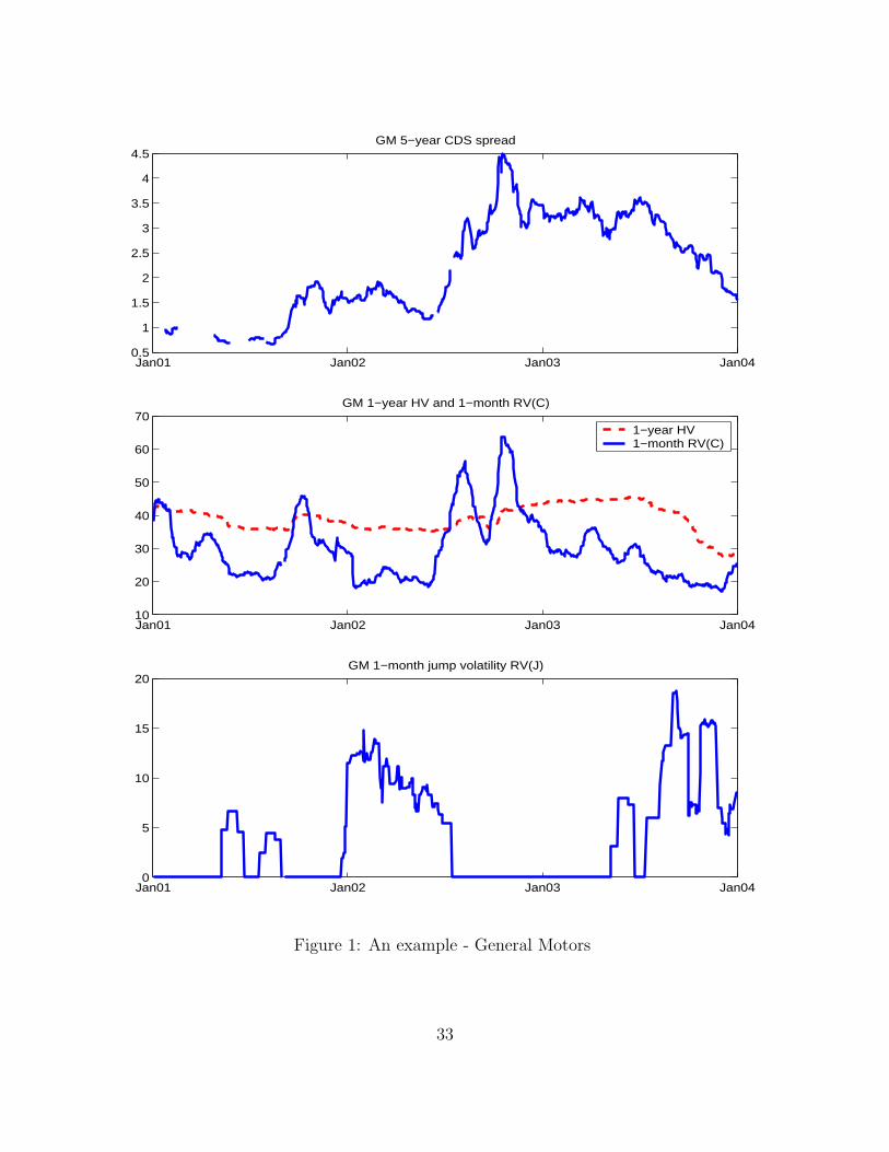
CDS spreads exhibit substantial time variation and cross-section difference in our sample.

Typically CDS spreads increased substantially in the first half of year 2002, and then declined

gradually throughout the remaining sample period (see Figures 1 and 2 for an example). By

rating categories the average CDS spread for single-A to triple-A entities is 45 basis point,

whereas the average spreads for triple-B and high-yield names are 116 and 450 basis points,

respectively.

9

3.2 Individual volatility

Throughout this paper we use two sets of measures for equity volatility of individual firms:

historical volatility calculated from daily equity price and realized volatility calculated from

intra-day equity prices. Data sources are CRSP and TAQ respectively. CRSP provides daily

equity prices that are listed in the US stock market, and TAQ (Trade and Quote) includes

intra-day (5-minute tick-by-tick) transactions data for securities listed on the NYSE, AMES

and NASDAQ.

We adopt the methods introduced in Section 2 to calculate historical volatility and real-

ized volatility (RV). For realized volatility we also decompose it into continuous (BV) and

jump (J) components by defining “jumps” at significance levels of 50%, 99% and 99.9%

(Equation 10) respectively.

The summary statistics of firm-level volatilities are reported in Table (2).12 The average

daily return volatility is between 2.1 − 2.7%, which is quite consistent by both measures.

Historical skewness varies by entities and by sample period, but its average is not significantly

different from zero over all time horizons from one week to one year. Using the truncated

measure of jumps defined in Equation (8), the jump component contributes about one quarter

of the total realized volatility.

Table (2) links the two measures of equity return volatility by calculating the correlation

coefficients between RV and historical volatility, between BV and historical volatility, and

between J and historical skewness. It is obvious that historical volatility is closely related

to realized volatility over the the long-term horizon, but their correlation becomes much

smaller for short sample period (such as one week). This is consistent with the prevalent

observation that realized volatility is a superior measure of short-term volatility, but this

gain disappears when the time horizon of interest increases. Another interesting finding is

the very low correlation (slightly negative in most cases) between J and historical skewness.

This is quite surprising at a first glance, since both measures have been proposed as proxy

for the jump process in asset value dynamics (Equation 2). On a second thought, the two

variables might have caught two different aspects of the jump process. Historical skewness

measures the asymmetry of extremely upward and downward movements in asset returns.13

12All volatility measures are represented by their squared root, i.e. as the standard deviation term.13Statistically, there is not clear connection between skewness and jumps. If the skewness is large and

positive, it implies that an extreme upward movement is more likely to occur. On the contrary, existence ofa jump process does not necessarily have any impact on skewness. For example, if upward and downwardjumps are equally likely to occur, the skewness is always zero.

10

In contrast, J is defined as the contribution of the jump component to the realized volatility.

Its magnitude is therefore related to the volatility of the jump. The two characteristics

of the jump process turn out to be not correlated with each other and may have different

implications on the pricing of credit risk.

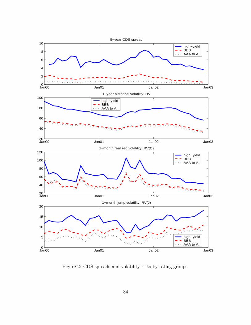
We also plot the time series of the above volatility measures and jump measures for the

General Motors (Figure 1) and for three rating groups (Figure 2). At a first glance, equity

returns of high-yield entities are more volatile and more likely to be affected by jumps. And

changes in credit spreads seem to move together with equity return volatility and jumps.

3.3 Firms’ balance sheet information

The firm’s balance sheet information is available from Compustat. Since it is reported on

a quarterly basis, the last available quarterly observations are used to estimate monthly

figures. We include the following explanatory variables:

1. Firm leverage. For each entity, market values of firm equity and book values of firm

debt are used to obtain leverage ratios, which are defined as

leverage =100 ∗ (Current debt + Long − term debt)

Total equity + Current debt + Long − term debt

The Merton’s framework predicts that a firm defaults when its leverage ratio ap-

proaches one. Therefore, it is clear that credit spreads tend to increase with leverage.

2. Return on equity (ROE). The item is defined as the ratio of pre-tax income to total

equity, which measures the profitability of the reference entity. When ROE is higher,

firm value is more likely to increase, therefore the default risk becomes smaller.

3. Coverage ratio. It measures the firm’s ability to pay back its outstanding debt, hence

tends to have a negative effect on the level of credit spreads. Its definition is

Coverage ratio = 100 ∗ OIBD − Depreciation

Interest expense + Current Debt

where OIBD denotes operating income before depreciation.

4. Dividend payout ratio. It is defined as the percentage ratio of dividend payout per

share by ex-date divided by equity price. A higher dividend payout ratio means a

11

decrease in asset value, therefore a default is more likely to occur and credit spreads

will increase.

Table (1) (lower left) includes summary statistics of the above variables. It is clear that

there are substantial variation of firm performance in our sample dataset.

3.4 Macro-financial variables

Following the prevalent practice in existing literature, we also include the following macro-

financial variables as explanatory variables of credit spreads. The data are obtained from

Bloomberg.

1. Changes in business climate. We use the S&P 500 average daily return, and its volatility

(in standard deviation term) in the last three months to proxy for the overall state of

the economy. Higher market returns and lower market volatility mean an improved

economic environment. Hence the two variables have negative and positive effects on

CDS spread, respectively.

2. 3-Month Treasury rate. A higher risk-free rate increases the risk-neutral drift of the

firm value process, therefore reducing the probability of default and the credit spreads.

However, a higher risk-free rate may also reflect the tightening of monetary policy,

which increases the firm’s cost of funding and weakens its ability to pay debt. The two

effects may exist together and their net impact is ambiguous.

3. Slope of the yield curve, which we define as the difference between the 10-year and

3-month US Treasury rates. An increase in yield curve slope implies an increase in

expected future short rate or an improved economic condition in the future. By the

same argument as above, it should lead to a decrease in credit spreads.

The summary statistics of these variables are reported in Table (1) (lower right portion).

4 Empirical evidence

Our empirical work focuses on the influence of equity return volatility and jumps on credit

spreads. We first run regressions with only jump and volatility measures. Then we also

include other control variables, such as ratings, macro-financial variables and balance sheet

12

information, as predicted by the structural models and evidenced by empirical literature.

Further robustness check with fixed effect and random effect does not affect result qualita-

tively. We also find strong interaction effect between jump/volatility measures with rating

variables and firm’s accounting information, suggesting that financial market risk measures

are related to the fundamental health of firms’ balance sheet. Finally, the apparent non-

linear effect of jump and volatility risks indicates that using aggregate volatility or rating

group measures may over or under estimate the true impact of volatility and jump on credit

spread.14

4.1 Volatility and jump effect on credit spread

Table 3 reports the main findings of ordinary least squares (OLS) regressions, which explain

credit spreads only by different measures of equity return volatility and/or jump measures.

Regression (1) using 1-year historical volatility alone reaches R-square 45%, which is higher

that the main result of Campbell and Taksler (2003, regression 8 in Table II, R-square 41%)

with all volatility, ratings, accounting information, and macro-finance variables combined

together. Regression (2) and (3) show that short term realized volatility also explain a

significant portion of spread variations, and that combined long-run (1-year HV) and short-

run (1-month RV) volatilities gives the best result of 50% R-square. The signs of coefficients

are all correct—high volatility raise credit spread, and the magnitudes are all sensible—

one percentage volatility shock raises credit spread about 3-9 basis points. The statistical

significance will remain even if we put in all other control variables (discussed in the following

subsection).

Our major contribution is to construct innovative jump measures and show that jump

risks are indeed priced in CDS spreads. Regression (4) suggests that historical skewness as a

measure of jump risk can have a correct sign (positive jumps reduce spreads), if we also add

the historical kurtosis variable with correct sign (more jumps increases spread). This is in

contrast with the counter-intuitive finding that skewness has a significantly positive impact

on credit spreads (Cremers et al 2004a). However, the total predictability of traditional

jump measure is still very dismal—only 3% in R-square. Our new measures of jumps—

regressions (5) to (7)—give significant estimates, and by themselves explain 23% of credit

spread variations. A few points are worth mentioning. First, the jump volatility has the

14In all regressions we focus on the 5-year CDS spread, and the results are similar for 1-year CDS andavailable upon request

13

strongest impact—raising default spread by 3-5 basis points for percentage increase. Second,

when jump mean effect (-0.2 basis point) is decomposed into positive and negative parts,

there is a strong asymmetry in that positive jumps only reduce spread by 0.5 basis point

but negative jumps can increase spread by 1.50 basis points. This is a new finding in the

empirical literature on credit risks. Third, average jump size only has mute effect (-0.2) and

jump intensity can switch sign (from 0.7 to -0.6), which may be explained by controlling for

positive or negative jumps.

Our new benchmark—regression (8) explains 53% of credit spread with volatility and

jump variables alone. To summarize, both long-run and short-run volatilities have significant

positive impacts, so do jump intensity, jump variance, and negative jump; while positive jump

reduces spread.

4.2 Extended regression with traditional controlling variables

We then include more explanatory variables—credit ratings, macro-financial conditions and

firm’s balance sheet information—all of which are theoretic determinants of credit spreads

and have been widely used in previous empirical studies. The regressions are implemented

in pairs, one with and the other without measures of volatility and jump. Table 4 reports

the results.

In the first exercise, we examine the extra explanatory power of equity return volatility

and jump in addition to ratings. Cossin and Hricko (2001) suggest that rating information

is the single most important factor in determinant CDS spreads. Indeed, our results confirm

their findings that rating information alone explains about 57% of the variation in credit

spreads. But this is about the same as the volatility and jump effects alone (see table 3). A

remarkable result is that, volatility and jump risks can explain another 16% of the variation

(R2 increases to 73%).

The increase in R2 is also very large in the second pair of regressions. Regression (3) shows

that all other variables, including macro-financial factors (market return, market volatility,

yield curve level and slope), firm’s balance sheet information (ROE, firm leverage, coverage

and dividend payout ratio) and the recovery rate used by price providers, combined explain

an additional 6% of credit spread movements on the top of rating information (regression (3)

minus regression (1)). The combined impact increase is smaller than the volatility and jump

effect (16%). Moreover, regression (4) suggests that the inclusion of volatility and jump

effect provides another 12% explanatory power compared to regression (3). R2 increases to

14

a very high level of 0.75. The results suggest that the volatility effect is independent of the

impact of other structural or macro factors.

The jump and volatility effects are very robust, with the same signs and little change in

magnitudes. To gauge the economic significance more systemically, it is useful to go back to

the summary statistics presented earlier (Table 2). The cross-firm average of the standard-

deviation of the 1-year historical volatility and the 1-month realized volatility (continuous)

are 38.35% and 44.20%, respectively. Such shocks lead to a widening of the credit spreads

by almost 107-128 and 73-87 basis points, respectively. Finally, consider jump variance only,

one standard deviation shock (9.03%) increase credit spreads by 11-14 basis points. If we

include jump intensity, positive and negative jumps, the total jump impact on credit spreads

is like in the same order as the volatility impact.

Judging from the full model of regression (4), some macro-financial factors and firm

variables have the expected signs of the slope coefficients. The market return has a significant

negative impact on the spreads, consistent with the business cycle effect. High leverage ratio

tends to increase credit spread significantly, which is consistent with structural model insight.

All other variables seem to have either marginal t-statistics or economically counter-intuitive

signs, and their signs & magnitudes seem to be unstable depending on whether we include

volatility and jump variables or not. It is worth pointing out that the statistical significance

of firm level volatility and jump risks are uniformly higher than the credit ratings, which

used to be considered as the most influential factors (Cossin and Hricko 2001).

4.3 Robustness Check

We also implement a robustness check by using panel data technique with fixed and random

effects (see Table (5)). Although Hausman test favors fixed effects over random effects,

the regression results do not differ much between these two approaches. In particular, the

slope coefficients of the individual volatility and jump variables are remarkably stable and

qualitatively unchanged. On the other hand, only some of the macro-financial and firm

accountings variables have consistent and significant impacts on credit spreads, including

market return (negative), term spread (positive), leverage ratio (positive), and dividend

payout (positive). Although notice that fixed effects or random effects can drive the rating

dummies to be marginally insignificant, and the high R-square of 87% is caused by the two

hundreds or so firm dummies.

15

4.4 Interaction with rating group and accounting information

We have demonstrated that equity volatility and jump helps to determine the credit spreads.

There remain questions of whether the effect is merely a statistical phenomenon or intimately

related to firm’s credit standing and accounting fundamental, whether the effect is non-

linear in nature, and whether different components of equity volatility have different price

implications. The next three sub-sections aim to address the three issues respectively.

We first examine whether the volatility effect varies across different rating classes. Figure

(2) shows that the equity return volatility and especially jump volatility are much different

across rating groups. Not surprisingly, high-yield names are associated with higher risk and

therefore more volatile credit spreads. This suggests that, for the same coefficient size, the

economic implication of the volatility effect is more remarkable for high-yield entities. Table

(6) examines this issue more seriously in regression (1) across three rating groups: triple-A

to single-A names, triple-B names and high-yield entities. The results are remarkable in that

the volatility/jump impact coefficients from high yield entities are typically several multiples

larger than for the investment grade names. To be more precise, for long-run volatility the

difference is 4.69 over 2.28, short-run volatility 2.53 over 0.37, jump intensity 2.70 over 1.19,

jump volatility 3.92 over 0.58, and positive jump -1.08 over -0.24. Similarly the t-ratios of

high-yield interaction terms are also much larger than those of the investment grade. In

addition, these differences seem to be much larger for the realized volatility and jump risk

measures, than for the historical volatility measure, which further justifies our approach of

identifying volatility and jump risks separately from high frequency data.

Our measures on jumps and volatilities interact strongly with the firm specific accounting

information. As shown by regression (2) in Table (6), the interactions between leverage

ratio and various volatility and jump measures tend to increase the credit risk spreads,

while recovery rate tends to have opposite interaction effects with long-run versus short-

run volatilities and with different jump measures. Other variables like return to equity and

dividend payout also have significant interactions with volatility and jump risk measures, but

their signs and significances are less uniform. Nevertheless, the combined explanatory power

of credit spreads reaches a R-square of 80%. These results reinforce the idea that volatility

and jump risks are priced in the CDS spreads, not only because there are statistical linkages,

but also because equity market trades on the firms’ fundamental information. In particular,

the time-varying recovery rate issue can be re-examined as the co-movement between quoted

recovery rate and volatility/jump risk measures.

16

4.5 Nonlinear effect and credit premium puzzle

While the theory usually implies a complicated relationship between volatility and credit

spreads, in empirical exercise a simplified linear relationship is often used. This linear ap-

proximation could cause substantial bias in calibration exercise and partly contribute to the

under-performance of structural model, or the so-called credit premium puzzle. For instance,

in Huang and Huang’s (2003) paper, they used the average equity volatility within a rating

class in their calibration, and found that the predicted credit spread is much lower than

the observed value (average credit spreads in the rating class). However, the “averaging” of

individual equity volatility could be problematic if its impact on credit spread in non-linear.

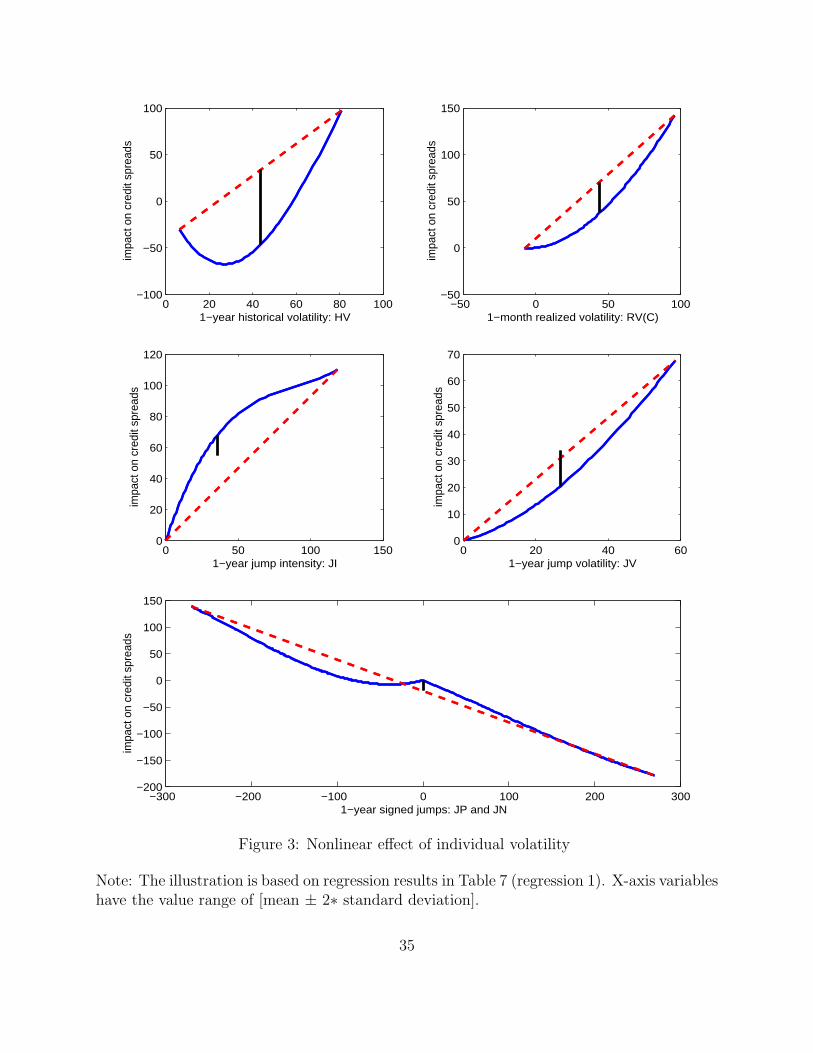
Table (7) confirms the non-linearity effect of volatility and jump. By adding the squared

and cubic terms of the jump and volatility risk measures, we find that most of the nonlinear

terms are statistically significant. The sign of each order may not be quite integrable, since

the entire nonlinear function is driving the impact. Figure (3) illustrates the potential impact

of this “Jensen inequality” problem on the performance of price prediction. If we use the

mean rather than individual volatility in the calibration, the predicted credit spreads could

be lower than the true average credit spread by as much as 81 (due to 1-year historical

volatility) and 33 (due to 1-month realized volatility) basis points, which goes a long way

to resolve the under-prediction part of the credit premium puzzle. Likewise, using the mean

rather than individual jump intensity and volatility, the predicted CDS spreads would be

13 basis points higher (due to 1-year jump intensity), cancelling out 13 basis points lower

(due to 1-year jump volatility). Most interesting is the signed jumps—in negative region

averaging may under-predict credit spreads but in positive region over predict, with overall

small over-prediction of 4 basis points. In short, averaging volatilities over individual firms

produces significant underfitting of credit yield curve, while averaging jumps may cancel

each other out the nonlinear effect.

5 Simulation evidence from stylized models

Our findings of predictability of volatility and jump risks for credit spreads are qualitatively

consistent with the structural model implications. At the same time, we know that the

structural approaches have difficulties in matching the observed credit spreads. In this

section, we examine the capability of a standard model of Merton (1974) and a stochastic

volatility model in replicating the forecast-ability of historical volatility for credit premium.

17

We also illustrate the flexibility of credit yield curves from the time-varying volatility model.

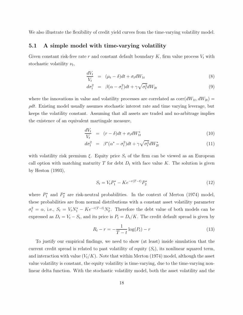
5.1 A simple model with time-varying volatility

Given constant risk-free rate r and constant default boundary K, firm value process Vt with

stochastic volatility νt,

dVt

Vt= (µt − δ)dt + σtdW1t (8)

dσ2t = β(α − σ2

t )dt + γ√

σ2t dW2t (9)

where the innovations in value and volatility processes are correlated as corr(dW1t, dW2t) =

ρdt. Existing model usually assumes stochastic interest rate and time varying leverage, but

keeps the volatility constant. Assuming that all assets are traded and no-arbitrage implies

the existence of an equivalent martingale measure,

dVt

Vt= (r − δ)dt + σtdW ∗

1t (10)

dσ2t = β∗(α∗ − σ2

t )dt + γ√

σ2t dW ∗

2t (11)

with volatility risk premium ξ. Equity price St of the firm can be viewed as an European

call option with matching maturity T for debt Dt with face value K. The solution is given

by Heston (1993),

St = VtP∗1 − Ke−r(T−t)P ∗

2 (12)

where P ∗1 and P ∗

2 are risk-neutral probabilities. In the context of Merton (1974) model,

these probabilities are from normal distributions with a constant asset volatility parameter

σ2t = α, i.e., St = VtN

∗1 − Ke−r(T−t)N∗

2 . Therefore the debt value of both models can be

expressed as Dt = Vt − St, and its price is Pt = Dt/K. The credit default spread is given by

Rt − r = − 1

T − tlog(Pt) − r (13)

To justify our empirical findings, we need to show (at least) inside simulation that the

current credit spread is related to past volatility of equity (St), its nonlinear squared term,

and interaction with value (Vt/K). Note that within Merton (1974) model, although the asset

value volatility is constant, the equity volatility is time-varying, due to the time-varying non-

linear delta function. With the stochastic volatility model, both the asset volatility and the

18

delta function are time-varying.

5.2 Simulation evidence from structural models

In the Monte Carlo exercise, we set the annualized parameters as following: β = 0.10,

α = 0.25, γ = 0.10, ξ = −0.20, and ρ = −0.50. To focus on stochastic volatility, we set

non-essential parameters to zero, i.e., µt = δ = r = 0. In addition, the starting value of

the asset is set at 100 and the debt boundary is set at 60. For each random sample, we

simulate 10 years of daily realization, and then calculate the monthly variables similar to

the empirical exercise. We perform regression analysis between current month credit spread

and lagged one year volatility, nonlinear volatility term, and interaction between volatility

and asset value change. The total Monte Carlo replications is 2000 random samples. The

results are shown in the following Table (8).

It is clear that even with the Merton (1974) model, equity volatility and volatility squared

show strong predictability for credit risk premia, with R-square around 0.57 and positive

signs largely consistent with our empirical findings. Also note that the interaction term of

equity volatility and firm value change is negatively impacting the credit spread, which is

also consistent with our empirical evidence in Table 6 on historical volatility and recovery

rate. It should be point out that within Merton (1974) model the asset volatility is constant.

However the equity volatility is time-varying due to the fact that the nonlinear delta function

is depending on the time-varying firm value. Our justification of time-varying volatility effect

on credit spread is completely opposite to that of Campbell and Taksler (2003), who assume

that debt is risk-free and that delta function is constant.

As seen from Table (8), a stochastic volatility model produces similar predictability R-

squares and coefficient signs, for the default risk premium from equity volatility, nonlinear

term, and interaction term. However, coefficient magnitudes are 2-10 times larger than the

constant volatility model, and t-ratios parameter estimates are also slightly higher than the

Merton (1974) model. Both the nonlinear and the interaction terms have similar sign as

we discovered in the empirical exercise. Also, the R-square of 0.51-0.57 from volatility and

R-square of 0.72-0,75 from volatility and interaction combined, match quite well as what we

have found in the actual CDS prediction regressions.

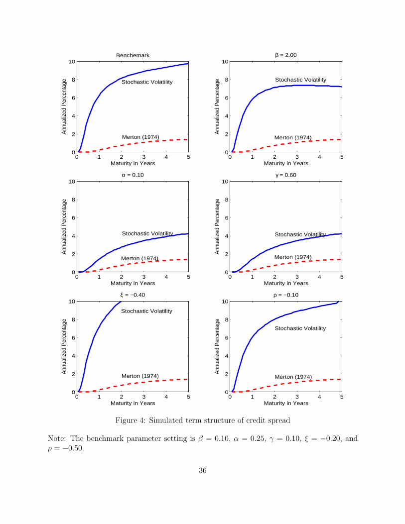
Figure (4) illustrate the difference between the credit yield curves from a stochastic

volatility model and the Merton (1974) model. In the benchmark case (upper left), both

models have the same unconditional volatility. The Merton (1974) model credit curve is very

19

flat (less than 200 basis points) while the stochastic volatility yield curve is much steep (close

to 1000 basis points). By changing the underlying model parameters, the credit curve from

time-varying volatility model can assume a variety shapes—flat, steep, hump, straight, etc..

Such a flexibility may potentially overcome under-fitting problem of the standard structural

model, and may price the individual credit spread more accurately.

6 Conclusions

In this paper we use a large dataset to examine the impact of theoretic determinants, par-

ticularly firm-level equity return volatility and jumps, on the level of credit spreads in the

credit-default-swap market. Our results find strong volatility and jump effect, which explains

another 12% of the movements in credit spreads after controlling for rating information and

other structural factors. In particular, when all these control variables are included, equity

volatility and jumps are still the most significant factors, even more than the rating infor-

mations. This effect is economically significant and remains robust to a number of variants

of the estimation method. The volatility and jump effects are the strongest for high-yield

entities, and they also exhibit strong non-linearity for investment-grade names. We expect

that the non-linearity could be used to explain the under-performance of structural models

in the existing literature.

We adopt an innovative approach to identify return jumps of individual firms, which

enables us to assess the impact of various jump risks (intensity, variance, negative jumps)

on default risk premia. Our results on jumps are statistically and economically significant,

which contrasts the typical mixed finding in literature using historical or implied skewness

as jump proxy.

Our study is only a first step towards improving our understanding of the impact of

volatility and jumps on credit risk pricing. Calibration exercise that takes into the time

variation of volatility & jump risks and the non-linear effect could be a promising direction

to explore for resolving the so-called credit premium puzzle. Related issues, such as the

connections between equity volatility and asset volatility, also worth more attention from

academic researchers and practitioners.

20

References

[1] Amato, J. and E. Remolona (2003): “The credit premium puzzle”, BIS Quarterly

Review, December, pp 51-63.

[2] Anderson R., S. Sundaresan and P. Tychon (1996): “Strategic analysis of contingent

claims”, European Economic Review, vol 40, pp 871-81.

[3] Andersen, T. and T. Bollerslev (1998): “Answering the skeptics: yes, standard volatil-

ity models do provide accurate forecasts”, International Economic Review, vol 39, pp

885-905.

[4] Andersen, T., T. Bollerslev and F. Diebold (2003): “Parametric and Non-Parametric

Volatility Measurement”, in Handbook of Financial Econometrics (L. P. Hansen and

Y. Aıt-Sahalia, eds.), Elsevier Science, New York, forthcoming.

[5] —— (2004): “Some like it smooth, and some like it rough: untangling continuous and

jump components in measuring, modeling, and forecasting asset return volatility”,

working paper.

[6] Andersen, T., T. Bollerslev, F. Diebold and P. Labys (2001): “The distribution of

realized exchange rate volatility”, Journal of the American Statistical Association, vol

96, pp 42-55.

[7] Barndorff-Nielsen, O. and N. Shephard (2002a): “Econometric analysis of realized

volatility and its use in estimating stochastic volatility models”, Journal of the Royal

Statistical Society, vol 64, pp 253-80.

[8] —— (2002b): “Estimating quadratic variation using realized variance”, Journal of

Applied Econometrics, vol 17, pp 457-78.

[9] —— (2003a): “Realised Power Variation and Stochastic Volatility”, Bernoulli, vol 9,

pp 243-265.

[10] —— (2003b), “Econometrics of Testing for Jumps in Financial Economics Using

Bipower Variation”, working paper, Oxford University.

[11] —— (2004): “Power and bipower variation with stochastic volatility and jumps”,

Journal of Financial Econometrics, vol 2, pp 1-48.

[12] Blanco, R., S. Brennan and I. W. March (2004): “An empirical analysis of the dynamic

relationship between investment-grade bonds and credit default swaps”, Bank of Spain

Working Paper no 0401.

21

[13] Campbell, J. and G. Taksler (2002): “Equity volatility and corporate bond yields”,

working paper.

[14] Collin-Dufresne, P. and R. Goldstein (2001): “Do credit spreads reflect stationary

leverage ratios?”, Journal of Finance, vol 56, pp 1929-57.

[15] Collin-Dufresne, P., R. Goldstein and S. Martin (2001) : “The determinants of credit

spread changes”, Journal of Finance, vol LVI, no 6, pp 2177-2207.

[16] Collin-Dufresne, P., R. Goldstein and J. Helwege (2003): “Is credit event risk priced?

Modeling contagion via the updating of beliefs”, working paper.

[17] Cossin, D. and T. Hricko (2001): “Exploring for the determinants of credit risk in

credit default swap transaction data”, working paper.

[18] Cremers, M., J. Driessen, P. Maenhout and D. Weinbaum (2004a): “Individual stock-

option prices and credit spreads”, Yale ICF Working Paper no 04-14.

[19] —— (2004b): “Explaining the level of credit spreads: option-implied jump risk premia

in a firm value model”, working paper.

[20] Eom, Y. H., J. Helwege and J. Huang (2004): “Structural models of corporate bond

pricing: an empirical analysis”, Review of Financial Studies, vol 17, no 2, pp 499-544.

[21] Eraker, B., B. Johannes and N. Polson (2003): “The impact of jumps in volatility and

returns”, Journal of Finance, vol 58, pp 1269-1300.

[22] Houweling, P. and T. Vorst (2003):“Pricing default swaps: empirical evidence”, Journal

of International Money and Finance, forthcoming.

[23] Huang, J. and M. Huang (2003): “How much of the corporate-treasury yield spread is

due to credit risk?”, working paper.

[24] Huang, X. and G. Tauchen (2004): “The relative contribution of jumps to total price

variance”, Duke University working paper.

[25] Hull, J., M. Predescu and A. White (2003): “The relationship between credit default

swap spreads, bond yields, and credit rating announcements”, working paper, Univer-

sity of Toronto.

[26] Kassam, A. (2003): “Options and volatility”, Goldman Sachs Derivatives and Trading

Research Report, January.

[27] Kou, S. G. and H. Wang (2003): “First passage times of a jump diffusion process”,

Advanced Applied Probability, vol 35, p 504-31.

22

[28] Leland, H. E. (1994): “Corporate debt value, bond covenants, and optimal capital

structure”, Journal of Finance, vol 49, no 4, pp 1213-52.

[29] Leland, H. E. and K. B. Toft (1996): “Optimal capital structure, endogenous

bankruptcy, and the term structure of credit spreads”, Journal of Finance, vol 51,

no 3, pp 987-1019.

[30] Longstaff, F. and E. Schwartz (1995): “A simple approach to valuing risky fixed and

floating rate debt”, Journal of Finance, vol 50, pp 789-820.

[31] Longstaff, F., S. Mithal and E. Neis (2004): “Corporate yield spreads: default risk or

liquidity? new evidence from the credit-default-swap market”, NBER working paper

no 10418.

[32] Meddahi, N. (2002): “A Theoretical Comparison Between Integrated and Realized

Volatility”, Journal of Applied Econometrics, vol 17, pp 479-508.

[33] Mella-Barral P. and W. Perraudin (1997): “Strategic debt service”, Journal of Finance,

vol 52, pp 531-66.

[34] Merton, R. (1974): ”On the pricing of corporate debt: the risk structure of interest

rates”, Journal of Finance, vol 29, pp 449-70.

[35] Pan, J (2001): “The jump-risk premia implicit in options: evidence from an integrated

time-series study”, Journal of Financial Economics, vol 63, pp 3-50.

[36] Zhou, C. (1997): “A jump-diffusion approach to modeling credit risk an valuing de-

faultable securities”, Federal Reserve Board Finance and Economic Discussion Series

1997-15.

[37] Zhou, C. (2001): “The term structure of credit spreads with jump risk”, Journal of

Banking and Finance, vol 25, pp 2015-40.

[38] Zhu, H. (2004): “An empirical comparison of credit spreads between the bond market

and the credit default swap market”, BIS Working Paper no 160.

23

7 Appendix (to be completed)

24

Table 1: Summary Statistics: (i) sectoral distribution of sample entities; (ii) distribution of credit spread observationsby ratings; (iii) firm-specific information; (iv) macro-financial variables.

By sector number percentage (%) By rating number percentage (%)

Communications 20 6.51 AAA 219 2.15Consumer cyclical 63 20.52 AA 559 5.48Consumer Stable 55 17.92 A 3052 29.92Energy 27 8.79 BBB 4394 43.07Financial 23 7.49 BB 1321 12.95Industrial 48 15.64 B 544 5.33Materials 35 11.40 CCC and below 112 1.10Technology 14 4.56Utilities 18 5.88Not specified 4 1.30Total 307 100 Total 10201 100Firm-specific variables Mean Std. dev. Macro-financial variables Mean (%) Std. dev.Recovery rates (%) 39.50 4.63 S&P 500 return -13.15 14.72Return on equity (%) 4.50 6.80 S&P 500 vol 22.42 2.90Leverage ratio (%) 48.81 18.64 3-M Treasury rate 2.04 1.24Coverage ratio (%) 125.94 209.18 Term spread 2.51 0.96Div. Payout ratio (%) 0.41 0.475-year CDS spread (bps) 172 2301-year CDS spread (bps) 157 236

25

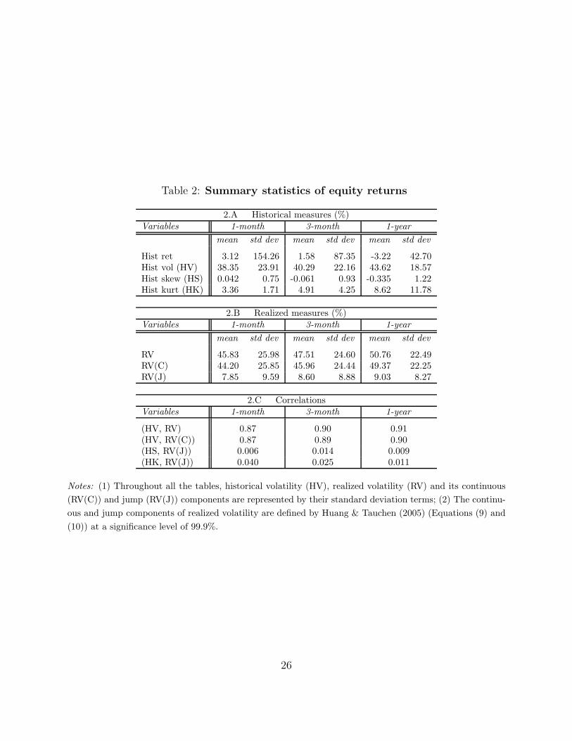
Table 2: Summary statistics of equity returns

2.A Historical measures (%)Variables 1-month 3-month 1-year

mean std dev mean std dev mean std dev

Hist ret 3.12 154.26 1.58 87.35 -3.22 42.70Hist vol (HV) 38.35 23.91 40.29 22.16 43.62 18.57Hist skew (HS) 0.042 0.75 -0.061 0.93 -0.335 1.22Hist kurt (HK) 3.36 1.71 4.91 4.25 8.62 11.78

2.B Realized measures (%)Variables 1-month 3-month 1-year

mean std dev mean std dev mean std dev

RV 45.83 25.98 47.51 24.60 50.76 22.49RV(C) 44.20 25.85 45.96 24.44 49.37 22.25RV(J) 7.85 9.59 8.60 8.88 9.03 8.27

2.C CorrelationsVariables 1-month 3-month 1-year

(HV, RV) 0.87 0.90 0.91(HV, RV(C)) 0.87 0.89 0.90(HS, RV(J)) 0.006 0.014 0.009(HK, RV(J)) 0.040 0.025 0.011

Notes: (1) Throughout all the tables, historical volatility (HV), realized volatility (RV) and its continuous(RV(C)) and jump (RV(J)) components are represented by their standard deviation terms; (2) The continu-ous and jump components of realized volatility are defined by Huang & Tauchen (2005) (Equations (9) and(10)) at a significance level of 99.9%.

26

Table 3: Baseline regression: explaining 5-year CDS spreads using individual equity volatilities and jumps

Dependent variable: 5-year CDS spread (in basis point)

Explanatory variables 1 2 3 4 5 6 7 8

Constant -207.22 -91.10 -223.11 147.35 169.29 85.66 20.80 -273.46(36.5) (18.4) (40.6) (39.6) (50.3) (20.8) (3.9) (42.8)

1-year HV 9.01 6.51 6.90(72.33) (40.2) (38.8)

1-year HS -10.23(3.2)

1-year HK 2.59(7.5)

1-month RV 6.04 2.78(60.5) (23.0)

1-month RV(C) 2.37(20.2)

1-year JI 0.71 -0.65 1.46(9.5) (5.0) (13.4)

1-year JM -0.21(15.8)

1-year JV 5.21 3.44 1.20(32.9) (14.4) (6.3)

1-year JP -0.45 -0.67 -0.62(7.3) (9.8) (11.8)

1-year JN 1.47 1.56 0.45(22.9) (23.6) (8.3)

Adjusted R2 0.45 0.37 0.50 0.03 0.19 0.14 0.23 0.53Obs. 6342 6353 6337 6342 6064 6328 6064 6064

Notes: (1) t-statistics in the parenthesis; (2) JI, JM, JV, JP and JN refer to the jump intensity, jump mean, jump variance, positive jumpsand negative jumps as defined in section 2.

27

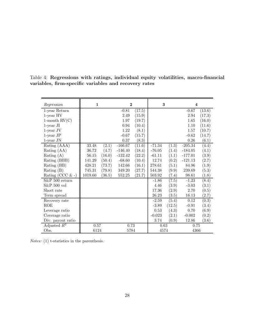
Table 4: Regressions with ratings, individual equity volatilities, macro-financialvariables, firm-specific variables and recovery rates

Regression 1 2 3 41-year Return -0.81 (17.5) -0.67 (13.6)1-year HV 2.49 (15.9) 2.94 (17.3)1-month RV(C) 1.97 (19.7) 1.65 (16.0)1-year JI 0.94 (10.4) 1.10 (11.6)1-year JV 1.22 (8.1) 1.57 (10.7)1-year JP -0.67 (15.7) -0.62 (14.7)1-year JN 0.37 (8.3) 0.26 (6.1)Rating (AAA) 33.48 (2.1) -166.67 (11.6) -71.34 (1.3) -205.34 (4.4)Rating (AA) 36.72 (4.7) -146.40 (18.4) -76.05 (1.4) -184.05 (4.1)Rating (A) 56.15 (16.0) -132.42 (22.2) -61.11 (1.1) -177.01 (3.9)Rating (BBB) 141.29 (50.4) -68.60 (10.4) 12.74 (0.2) -121.13 (2.7)Rating (BB) 428.21 (73.7) 142.66 (16.1) 278.61 (5.1) 84.96 (1.9)Rating (B) 745.31 (79.8) 349.20 (27.7) 544.38 (9.9) 239.69 (5.3)Rating (CCC & -) 1019.60 (36.5) 552.25 (21.7) 503.92 (7.4) 98.61 (1.8)S&P 500 return -1.86 (7.5) -1.23 (8.4)S&P 500 vol 4.46 (3.9) -3.03 (3.1)Short rate 17.36 (2.9) 2.70 (0.5)Term spread 26.23 (3.5) 16.13 (2.7)Recovery rate -2.59 (5.4) 0.12 (0.3)ROE -3.89 (12.5) -0.91 (3.4)Leverage ratio 0.53 (4.3) 0.70 (6.9)Coverage ratio -0.023 (2.1) -0.002 (0.2)Div. payout ratio 3.74 (0.9) 12.86 (3.6)Adjusted R2 0.57 0.73 0.63 0.75Obs. 6124 5784 4574 4366

Notes: (1) t-statistics in the parenthesis.

28

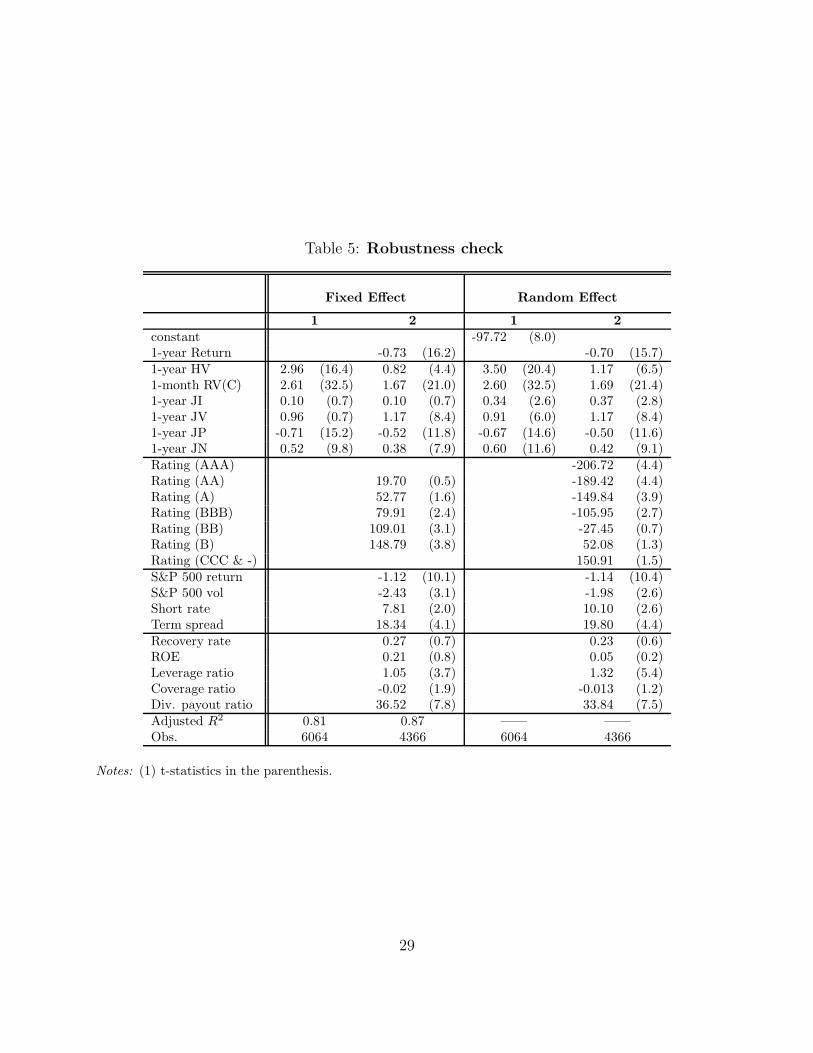
Table 5: Robustness check

Fixed Effect Random Effect

1 2 1 2constant -97.72 (8.0)1-year Return -0.73 (16.2) -0.70 (15.7)1-year HV 2.96 (16.4) 0.82 (4.4) 3.50 (20.4) 1.17 (6.5)1-month RV(C) 2.61 (32.5) 1.67 (21.0) 2.60 (32.5) 1.69 (21.4)1-year JI 0.10 (0.7) 0.10 (0.7) 0.34 (2.6) 0.37 (2.8)1-year JV 0.96 (0.7) 1.17 (8.4) 0.91 (6.0) 1.17 (8.4)1-year JP -0.71 (15.2) -0.52 (11.8) -0.67 (14.6) -0.50 (11.6)1-year JN 0.52 (9.8) 0.38 (7.9) 0.60 (11.6) 0.42 (9.1)Rating (AAA) -206.72 (4.4)Rating (AA) 19.70 (0.5) -189.42 (4.4)Rating (A) 52.77 (1.6) -149.84 (3.9)Rating (BBB) 79.91 (2.4) -105.95 (2.7)Rating (BB) 109.01 (3.1) -27.45 (0.7)Rating (B) 148.79 (3.8) 52.08 (1.3)Rating (CCC & -) 150.91 (1.5)S&P 500 return -1.12 (10.1) -1.14 (10.4)S&P 500 vol -2.43 (3.1) -1.98 (2.6)Short rate 7.81 (2.0) 10.10 (2.6)Term spread 18.34 (4.1) 19.80 (4.4)Recovery rate 0.27 (0.7) 0.23 (0.6)ROE 0.21 (0.8) 0.05 (0.2)Leverage ratio 1.05 (3.7) 1.32 (5.4)Coverage ratio -0.02 (1.9) -0.013 (1.2)Div. payout ratio 36.52 (7.8) 33.84 (7.5)Adjusted R2 0.81 0.87 —— ——Obs. 6064 4366 6064 4366

Notes: (1) t-statistics in the parenthesis.

29

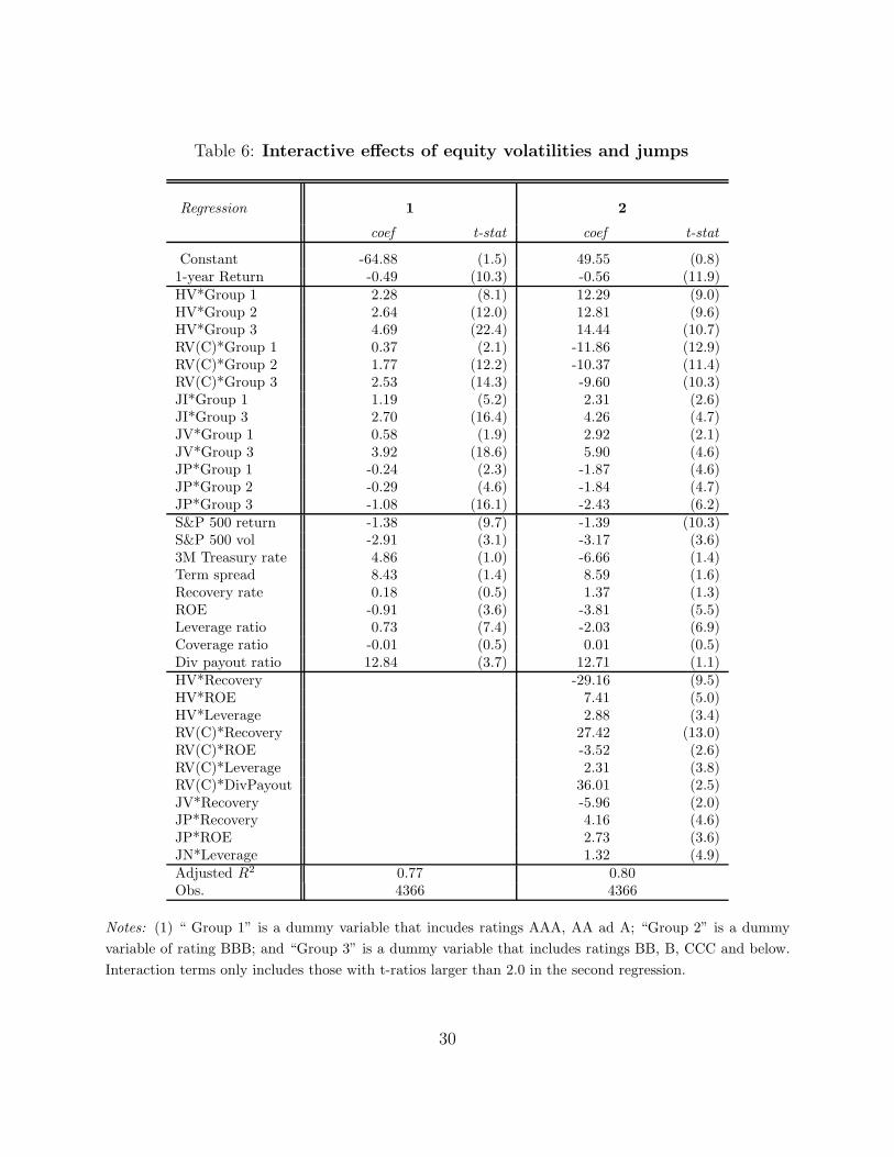
Table 6: Interactive effects of equity volatilities and jumps

Regression 1 2

coef t-stat coef t-stat

Constant -64.88 (1.5) 49.55 (0.8)1-year Return -0.49 (10.3) -0.56 (11.9)HV*Group 1 2.28 (8.1) 12.29 (9.0)HV*Group 2 2.64 (12.0) 12.81 (9.6)HV*Group 3 4.69 (22.4) 14.44 (10.7)RV(C)*Group 1 0.37 (2.1) -11.86 (12.9)RV(C)*Group 2 1.77 (12.2) -10.37 (11.4)RV(C)*Group 3 2.53 (14.3) -9.60 (10.3)JI*Group 1 1.19 (5.2) 2.31 (2.6)JI*Group 3 2.70 (16.4) 4.26 (4.7)JV*Group 1 0.58 (1.9) 2.92 (2.1)JV*Group 3 3.92 (18.6) 5.90 (4.6)JP*Group 1 -0.24 (2.3) -1.87 (4.6)JP*Group 2 -0.29 (4.6) -1.84 (4.7)JP*Group 3 -1.08 (16.1) -2.43 (6.2)S&P 500 return -1.38 (9.7) -1.39 (10.3)S&P 500 vol -2.91 (3.1) -3.17 (3.6)3M Treasury rate 4.86 (1.0) -6.66 (1.4)Term spread 8.43 (1.4) 8.59 (1.6)Recovery rate 0.18 (0.5) 1.37 (1.3)ROE -0.91 (3.6) -3.81 (5.5)Leverage ratio 0.73 (7.4) -2.03 (6.9)Coverage ratio -0.01 (0.5) 0.01 (0.5)Div payout ratio 12.84 (3.7) 12.71 (1.1)HV*Recovery -29.16 (9.5)HV*ROE 7.41 (5.0)HV*Leverage 2.88 (3.4)RV(C)*Recovery 27.42 (13.0)RV(C)*ROE -3.52 (2.6)RV(C)*Leverage 2.31 (3.8)RV(C)*DivPayout 36.01 (2.5)JV*Recovery -5.96 (2.0)JP*Recovery 4.16 (4.6)JP*ROE 2.73 (3.6)JN*Leverage 1.32 (4.9)Adjusted R2 0.77 0.80Obs. 4366 4366

Notes: (1) “ Group 1” is a dummy variable that incudes ratings AAA, AA ad A; “Group 2” is a dummyvariable of rating BBB; and “Group 3” is a dummy variable that includes ratings BB, B, CCC and below.Interaction terms only includes those with t-ratios larger than 2.0 in the second regression.

30

Table 7: Nonlinear effects of equity volatilities and jumps

Regression 1 2

coef t-stat coef t-stat

Constant -28.35 (1.4)1-year Return -0.25 (4.4) -0.68 (14.1)HV -3.14 (2.4) -5.34 (4.2)HV2 2.13 (6.6) 1.86 (5.4)HV3 -0.11 (4.6) -0.11 (3.9)RV(C) 0.25 (0.5) 0.18 (0.4)RV(C)2 0.37 (3.6) 0.26 (2.6)RV(C)3 -0.01 (2.8) -0.01 (1.3)JI 3.57 (6.1) 2.76 (5.9)JI2 -0.39 (3.9) -0.44 (5.2)JI3 0.01 (2.6) 0.03 (5.1)JV 2.18 (3.9) 0.36 (0.8)JV2 -0.40 (3.5) 0.26 (3.0)JV3 0.02 (4.3) -0.01 (2.9)JP -0.67 (3.6) -0.46 (3.0)JP2 -0.01 (0.7) -0.01 (1.0)JP3 0.001 (1.8) 0.0003 (1.1)JN -0.41 (2.1) -0.29 (2.0)JN2 0.09 (6.2) 0.06 (5.2)JN3 -0.002 (6.4) -0.001 (5.1)Rating (AAA) -107.06 (2.3)Rating (AA) -91.44 (2.0)Rating (A) -79.11 (1.7)Rating (BBB) -19.78 (0.4)Rating (BB) 184.36 (4.0)Rating (B) 301.08 (6.5)Rating (CCC & -) 254.63 (4.5)S&P 500 return -1.20 (8.4)S&P 500 vol -0.09 (0.1)3M Treasury rate 14.35 (3.0)Term spread 26.64 (4.6)Recovery rate -0.06 (0.2)ROE -1.20 (4.7)Leverage ratio 0.71 (7.3)Coverage ratio -0.001 (0.1)Div payout ratio 7.09 (2.1)Adjusted R2 0.57 0.78Obs. 6064 4366

Notes:

31

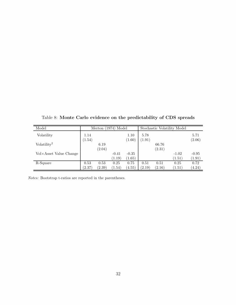
Table 8: Monte Carlo evidence on the predictability of CDS spreads

Model Merton (1974) Model Stochastic Volatility Model

Volatility 1.14 1.10 5.78 5.71(1.54) (1.60) (1.91) (2.06)

Volatility2 6.19 66.76(2.04) (2.31)

Vol×Asset Value Change -0.41 -0.35 -1.02 -0.95(1.19) (1.65) (1.51) (1.91)

R-Square 0.53 0.53 0.25 0.75 0.51 0.51 0.25 0.72(2.37) (2.39) (1.54) (4.55) (2.19) (2.16) (1.51) (4.24)

Notes: Bootstrap t-ratios are reported in the parentheses.

32

Jan01 Jan02 Jan03 Jan040.5

1

1.5

2

2.5

3

3.5

4

4.5GM 5−year CDS spread

Jan01 Jan02 Jan03 Jan0410

20

30

40

50

60

70GM 1−year HV and 1−month RV(C)

1−year HV1−month RV(C)


5

10

15

20GM 1−month jump volatility RV(J)

Figure 1: An example - General Motors

33


2

4

6

8

105−year CDS spread

high−yieldBBBAAA to A


40

60

80

1001−year historical volatility: HV



40

60

80

100

1201−month realized volatility: RV(C)



5

10

15

201−month jump volatility: RV(J)


Figure 2: CDS spreads and volatility risks by rating groups

34

0 20 40 60 80 100−100

−50

0

50

100

1−year historical volatility: HV

impa

ct o

n cr

edit

spre

ads

−50 0 50 100−50

0

50

100

150

1−month realized volatility: RV(C)

impa

ct o

n cr

edit

spre

ads

0 50 100 1500

20

40

60

80

100

120

1−year jump intensity: JI

impa

ct o

n cr

edit

spre

ads

0 20 40 600

10

20

30

40

50

60

70

1−year jump volatility: JV

impa

ct o

n cr

edit

spre

ads

−300 −200 −100 0 100 200 300−200

−150

−100

−50

0

50

100

150

1−year signed jumps: JP and JN

impa

ct o

n cr

edit

spre

ads

Figure 3: Nonlinear effect of individual volatility

Note: The illustration is based on regression results in Table 7 (regression 1). X-axis variableshave the value range of [mean ± 2∗ standard deviation].

35

0 1 2 3 4 50

2

4

6

8

10

Maturity in Years

Ann

ualiz

ed P

erce

ntag

eBenchemark

Merton (1974)

Stochastic Volatility

0 1 2 3 4 50

2

4

6

8

10

Maturity in Years

Ann

ualiz

ed P

erce

ntag

e

β = 2.00

Merton (1974)


0 1 2 3 4 50

2

4

6

8

10

Maturity in Years

Ann

ualiz

ed P

erce

ntag

e

α = 0.10

Merton (1974)


0 1 2 3 4 50

2

4

6

8

10

Maturity in Years

Ann

ualiz

ed P

erce

ntag

e

γ = 0.60

Merton (1974)


0 1 2 3 4 50

2

4

6

8

10

Maturity in Years

Ann

ualiz

ed P

erce

ntag

e

ξ = −0.40

Merton (1974)


0 1 2 3 4 50

2

4

6

8

10

Maturity in Years

Ann

ualiz

ed P

erce

ntag

e

ρ = −0.10

Merton (1974)


Figure 4: Simulated term structure of credit spread

Note: The benchmark parameter setting is β = 0.10, α = 0.25, γ = 0.10, ξ = −0.20, andρ = −0.50.

36

Explaining Credit Default Swap Spreads with Equity ...

Documents

Transcript of Explaining Credit Default Swap Spreads with Equity ...