Experimental Thermal and Fluid Science 34 (2010) 915–927

Contents lists available at ScienceDirect

Experimental Thermal and Fluid Science

journal homepage: www.elsevier .com/locate /et fs

Steady and unsteady flow within an axisymmetric tube dilatation

Ch. Stamatopoulos a, Y. Papaharilaou b, D.S. Mathioulakis a,*, A. Katsamouris c

a Department of Mechanical Engineering, Fluids Section, National Technical University of Athens, Greeceb Institute of Applied and Computational Mathematics, FORTH, Crete, Greecec Division of Vascular Surgery, Medical School, University of Crete, Greece

a r t i c l e i n f o

Article history:Received 23 November 2009Received in revised form 12 February 2010Accepted 20 February 2010

Keywords:Tube dilatationWall shearVortexFlow separation–reattachment

0894-1777/$ - see front matter � 2010 Elsevier Inc. Adoi:10.1016/j.expthermflusci.2010.02.008

* Corresponding author. Address: National Technicaof Mechanical Engineering, Fluids Section, 9 Heroon15710, Athens, Greece. Tel.: +30 210 7721020; fax: +

E-mail address: mathew@fluid.mech.ntua.gr (D.S.

a b s t r a c t

The flow field in an axisymmetric tube dilatation is studied employing a 2D PIV system and the commer-cial numerical code FLUENT. Experiment and numerical predictions are in good agreement providing sim-ilar trends and the same flow topology. For the steady case and for Re varying in the range 100–700, therecirculation zone length increases with Re, the flow reattachment line being displaced towards the exitof the model. Upstream of this line and a small distance from it, negative velocity maximizes close to thewall as well as the wall shear stress (in absolute value). Downstream of this region, the wall pressurepeaks and wall shear takes a local maximum at the model exit. In the rest part of the cavity both wallshear and pressure do not practically vary due to separated flow. The axial velocity on the longitudinalaxis of the model does not change streamwise for higher Re (Re = 690), resembling the near field of ajet, entraining fluid from the cavity region. In the unsteady case the flow rate is sinusoidal, the Womers-ley number is 3.3 and peak Re = 272. During early acceleration, a vortex ring is formed at the proximalpart of the cavity and two stagnation points appear on the longitudinal axis of the model approachingeach other as time progresses, eventually disappearing when the majority of the fluid particles changesdirection. The velocity profile at the exit is most of the cycle blunt compared to the parabolic type profileat the model entrance. In contrast to the steady case, the pressure variation does not exhibit a local peakwithin the cavity rather varying in a smooth way. Conversely, wall shear stress shows high peaks at thedistal end of the dilatation being proportional to the time dependent flow rate. The reattachment linetravels along the wall, as well as the local pressure peak which is always located downstream of it. Mass-less particles released at various locations and time instants within a cycle are not trapped in the recir-culation zone, being exposed to varying shear stress values.

� 2010 Elsevier Inc. All rights reserved.

1. Introduction

The objective of this work was to examine the flow in a tubedilatation both experimentally and numerically aiming at under-standing the fundamental fluid mechanics phenomena which oc-cur in arterial aneurysms. Due to severe implications on humanhealth following an aneurysm rupture, there has been a lot of effortby fluid mechanics researchers to reveal the etiology of the aneu-rysm formation and eventually its rupture, mainly from the hae-modynamic and in a lesser degree from a fluid–structureinteraction point of view. The time dependent blood flow rateand flow separation which takes place as a result of the suddenexpansion of the aneurysm make the flow field being quite com-plex. The problem becomes even more involved, if transition to

ll rights reserved.

l University of Athens, SchoolPolytechniou Ave., Zografos

30 210 7721057.Mathioulakis).

turbulence and relaminarization occurs within each cycle of theperiodic flow [1].

Rupture diagnosis of an arterial aneurysm and subsequently theneed for surgical treatment are of paramount importance for theclinicians. More particularly, abdominal aneurysms are consideredof high rupture risk when their maximum diameter exceeds 5 cmor their expansion rate is greater than 0.5 cm per year [2]. How-ever, according to clinical practice there have been cases that aneu-rysms have ruptured without following the above criteria [3–5].

There is strong evidence that growth and rupture of arterialaneurysms are related to haemodynamics since they appear at spe-cific locations of the vascular system. Wall shear stresses withinthe aneurysmal bulge are considered as the predominant factorfor arterial wall remodeling whereas static pressures are believedto be responsible for wall weakening, leading eventually to rupture[6]. Due to the increase of the arterial diameter, the flow separatesat the proximal edge, resulting in low negative wall shear stresses.In physiological flow waveforms these low stresses are additionallytime dependent, triggering a mechanism of blood particle adhesionto the arterial wall, like monocytes and platelets, causing thrombus

Nomenclature

d parental tube diameterD maximum model diameterL length of the modelpd downstream wall pressurepout wall pressure at the exit of the computational domainpin wall pressure at the inlet of the computational domainpw wall pressurep* nondimensional wall pressure, steady casep�un nondimensional wall pressure, unsteady caser radial coordinater* normalized radial coordinateRe Reynolds number

t time instantT period of a cycleu axial velocityx longitudinal axisa Womersley numberDp maximum pressure differencem kinematic viscositysrx fluid shear stresssst wall shear stress in straight tubesw wall shear stresss�w nondimensional wall shear stressx cyclic frequency

Fig. 1. Tube dilatation model. Dimensions in mm.

916 Ch. Stamatopoulos et al. / Experimental Thermal and Fluid Science 34 (2010) 915–927

formation [7]. In a recent study [8] on patients with intracranialaneurysms it was demonstrated that low wall shear stress regionsare associated with aneurysm growth. However, a comprehensivereview study by Lasheras [9] raises among other the intraluminalthrombus formation issue which cancels out the role of flow shearin the expansion of the aneurysm. Furthermore, this study providesa good explanation of the small progress that has been achieved sofar in answering questions with regard to aneurysm enlargementand rupture; namely, (a) the exact mechanism of flow shear onendothelium cells function is still unknown, (b) the mechanicalproperties of the arterial wall being nonlinear and anisotropic aredifficult to be determined especially due to remodeling, and (c)the present medical imaging techniques are not able to provideinformation about the wall thickness and its geometry with ade-quate accuracy.

During the last decade, a number of computational and experi-mental in vitro studies have been published aiming at providinginformation on the flow characteristics in either idealized or pa-tient-specific aneurysm shapes. The computational works treatnormally blood as a Newtonian fluid, while the flow rate is consid-ered either constant (steady flow) or time dependent. The em-ployed experimental techniques for velocity measurements aremainly 2D Particle Image Velocimetry [10–13] which allows forthe detection of coherent vortices translating on a lighted planeas well as Laser Doppler Velocimetry (LDV) for point measure-ments [14,15]. Normally, the aneurysm model walls are treatedas rigid and in few cases these are assumed to be compliant, study-ing the corresponding fluid–structure interaction problem [16–19].Also, flow visualization is used for qualitative study of the flow inaneurysms [20–23].

In the context of the present work a simple tube dilatationshape was chosen as a first step towards understanding the funda-mental mechanisms of blood motion in an aneurysm. Employing a2D PIV system the velocity field is simultaneously measured at agood number of points on a symmetry plane whereas ensembleaveraging is employed in the unsteady case. Numerical analysisis also used revealing valuable information of the flow close tothe wall where PIV fails to provide accurate results due to lightscattering.

The majority of the relevant works in the existing literature areeither numerical or experimental while very few of them use bothexperiment and numerical analysis. Especially, for time dependentflows in aneurysms, no such works have been published before, tothe best of our knowledge. Therefore, the present work aims to feelthis gap. Moreover, the objective of the present effort is the explo-ration of the basic flow characteristics which are more or less com-mon in aneurysms, like flow separation and reattachment, vortexformation, shear stress and pressure distributions. Knowing the ba-sic flow trends in a simple geometry it may help our understanding

of the flow behavior in nonsymmetric patient-specific models. Inorder to be able to draw solid conclusions, the examined Re andWomersley numbers were chosen to be relatively low to avoidthe appearance of flow instabilities. Wall shear stress and wall sta-tic pressure variations along the wall are presented and the differ-ences between steady and unsteady flow fields are revealed.Details of the flow reattachment region are shown as a functionof time as well as the moving wall pressure and shear stress peaks.

Although the used conditions in this work, namely rigid tubewalls, idealized tube dilatation shape, Re and Womersley numbersare not consistent with physiological flows in real aneurysms, thebasic flow field characteristics described here are similar with theresults of in vitro experiments in realistic aneurysm shapes andtheir numerical predictions.

2. Experimental method and model

The tube dilatation model is transparent, axisymmetric, of ellip-tical shape in the streamwise direction, made from an elastomermaterial (Sylgard-184) with a dilatation ratio D/d = 2.46 and elon-gation ratio L/d = 3.46, where D = 32 mm is the maximum diame-ter, d = 13 mm is the parental tube diameter and L = 45 mm is thelength of the model (Fig. 1). The above geometrical ratios are typ-ical for fusiform type aneurysms [15]. The model was manufac-tured of two identical half parts which were joined by pressingone against the other. The minimum thickness of the model wallswas 4 mm so that it was not deformed when time dependentpressures were applied. The model is connected, upstream anddownstream of it, to 600 mm long straight tubes of internal dia-meter d = 13 mm. This tube length is adequate in order for the flowto be fully developed when entering the model for all the examinedcases. More particularly, according to [24] the entrance length for astraight circular tube, assuming laminar steady flow, is given (intube diameters) by the formula [0.6191.6 + (0.0567Re)1.6]1/1.6.Therefore, for Re = 690, which was the maximum tested Re in thiswork, the entrance length is 39d = 507 mm. In the unsteady case,this length is time dependent and smaller than the entrance length

Fig. 2. Experimental set-up for the unsteady case.

Fig. 3. Computational domain and a portion of the numerical grid.

Ch. Stamatopoulos et al. / Experimental Thermal and Fluid Science 34 (2010) 915–927 917

that corresponds to peak Re (see [25,26]). Therefore, for the exam-ined peak Re = 272 this length is 234 mm.

The flow is established either by gravity when it is steady orsinusoidal for which a piston pump is used (Fig. 2). In the lattercase, in order to obtain a smooth flow rate waveform, an air–waterchamber is installed. The velocity field is measured on a symmetryplane of the model, employing a 2D PIV system (Oxford Lasers). Awater–glycerine solution (40/60 volume ratio) is used as the work-ing fluid in order to reduce image distortions due to the differenceof refraction indices at the fluid–solid interface. In order to reducelight scattering, the model is immersed in a bath of the same fluidcontained in a plexiglas tank. The viscosity of the solution wasmeasured with a viscometer (Cannon-Ubbelohde) and its densityby a hydrometer. The temperature of the fluid was kept constantwithin ±1 �C, so that its kinematic viscosity (8.11 cSt) did not varymore than 3.4%. The flow was seeded with 10 lm hollow glassspheres of neutral buoyancy (Potters Industries Inc.) and the flowrate was measured by an electromagnetic flow meter (CarolinaMedical, model FM501).

In the unsteady flow case, ensemble averaging is used, startingtaking images (t = 0) at a prescribed location of the reciprocatingpump piston through a noncontact sensor, based on eddy currentsprinciple. Fifty images are averaged for each instant to obtain agood statistical convergence. Cross correlation is performed forthe calculation of the particle displacements and 50% overlappingis employed along both directions. The interrogation windowsare 32 � 32 in size corresponding to an area of 1.1 � 1.1 mm2.The time interval between two consecutive images ranges between0.3 ms and 2.2 ms dependent on the flow rate.

Fig. 4. Bulk velocity versus time.

3. Numerical procedure

The flow field, assumed axisymmetric, was predicted using thecommercial code FLUENT, version 6.1.22 (Ansys Inc.). Half of thegeometric model (based on the experimental one), the used coor-dinate system (x, r) and a portion of the numerical grid are shownin Fig. 3. The lengths of the straight tubes connected to the aneu-rysm model are 677.5 mm, or 52 tube diameters each, being ade-quate for the flow to be fully developed (see previous paragraph).The computational domain is discretised with 295,972 quadrilat-eral elements, the numerical grid is unstructured in the bulge areaand structured in the straight tubes (Fig. 3). The closest node to thewall is 1% of the tube diameter far from it so that the wall velocitygradients are better calculated. This grid was selected following agrid independence test performing simulations with three differ-ent meshes with elements whose numbers varied between 105

and 3 � 105. Comparing the wall shear stress in the aneurysmbulge and axial velocity distributions, the thinner mesh predictionsdiffered from the coarser one (185,969 elements) by 1% at most,thus assuming that a converged solution was obtained. With

respect to the boundary conditions, a uniform velocity profile isconsidered at the entrance (left side of Fig. 3), fully developed con-ditions at the exit of the computational domain, no slip conditionsat the solid surfaces and symmetry conditions on the longitudinal

918 Ch. Stamatopoulos et al. / Experimental Thermal and Fluid Science 34 (2010) 915–927

model axis. In the unsteady case, the velocity at the entrance of thecomputational domain (x = �700 mm) is uniform and time depen-dent, based on the experimental flow rate (see Fig. 4) given by theformula u = �0.086 sin(xt + 0.609) + 0.0075 (m/s), where x is thecyclic frequency. An implicit first order scheme is implementedfor the time dependent terms with a time step of T/150, whereT = 3 s is the time period. Wall shear stress predictions based ona time step of T/100 deviated from those of T/150 with less than1% except for two stations, namely at the sharp edges that thebulge is connected to the straight tubes where the deviations didnot exceed 6% within the cycle. Since these deviations were onlylocal, it was assumed that the selected time step of T/150 doesnot affect the predictions of the whole flow field. The numericalsolution’s convergence for each time step was assumed when thenormalized residuals for continuity and momentum equationswas less than 10�7. A time periodic solution was obtained aftertwo cycles.

4. Results and discussion

4.1. Steady case

The flow field within the model, under steady inlet flow condi-tions, is examined for five Reynolds numbers, namely Re = 105,168, 206, 584 and 690. The common features of the above casesare flow detachment at the entrance of the model and reattach-

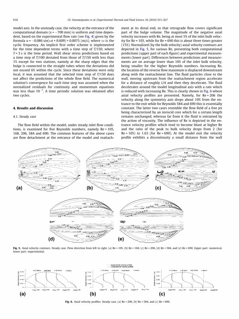
Fig. 5. Axial velocity contours. Steady case. Flow direction from left to right. (a) Re = 10lower part: experimental.

Fig. 6. Axial velocity profiles. Steady case. (a)

ment at its distal end, so that retrograde flow covers significantpart of the bulge volume. The magnitude of the negative axialvelocity increases with Re, being at most 5% of the inlet bulk veloc-ity for Re = 105, while for Re = 690 this is about three times greater(15%). Normalized (by the bulk velocity) axial velocity contours aredepicted in Fig. 5, for various Re, presenting both computationalpredictions (upper part of each figure) and experimental measure-ments (lower part). Differences between predictions and measure-ments are on average lower than 10% of the inlet bulk velocity,being smaller for the higher Reynolds numbers. Increasing Re,the location of the reverse flow maximum is displaced downstreamalong with the reattachment line. The fluid particles close to thewall, moving upstream from the reattachment region acceleratefor a distance of roughly L/4 and then they decelerate. The fluiddecelerates around the model longitudinal axis with a rate whichis reduced with increasing Re. This is clearly shown in Fig. 6 whereaxial velocity profiles are presented. Namely, for Re = 206 thevelocity along the symmetry axis drops about 10% from the en-trance to the exit while for Reynolds 584 and 690 this is essentiallyconstant. The latter two cases resemble the flow field of a free jetbeing characterized by an inviscid core which for a certain lengthremains unchanged, whereas far from it the fluid is entrained bythe action of viscosity. The influence of Re is depicted in the en-trance velocity profiles which tend to become blunt at higher Reand the ratio of the peak to bulk velocity drops from 2 (forRe = 105) to 1.63 (for Re = 690). At the model exit the velocityprofile exhibits a discontinuity a small distance from the wall

5, (b) Re = 168, (c) Re = 206, (d) Re = 584, and (e) Re = 690. Upper part: numerical,

Re = 206, (b) Re = 584, and (c) Re = 690.

Fig. 7. Velocity vectors. Steady case. (a) Re = 206 and (b) Re = 690. Upper part: numerical, lower part: experimental.

Fig. 8. Flow reattachment region. Velocity vectors. Steady case. (a) Re = 206 and (b) Re = 690.

Ch. Stamatopoulos et al. / Experimental Thermal and Fluid Science 34 (2010) 915–927 919

attributed to local fluid acceleration at the sharp junction of themodel to the exit straight tube. The flow entrainment is depictedin Fig. 7, where both velocity components are presented, namelythe radial component takes negative values in the area of theformed free shear layer. Approaching the exit of the model thiscomponent becomes positive since the flow is curved towardsthe reattachment region. This region is believed to be a probablesite of aneurysm rupture due to the high spatial velocity gradientswhich affect both the wall shear stress and wall pressure values ina way that the arterial wall strength is reduced [11]. Based on thecomputational results, the velocity vectors close to the flow reat-tachment region are shown in Fig. 8 for Re = 206 and 690 as wellas the locations of maximum wall pressure and wall shear. It is

Fig. 9. Wall pressure distribution. Steady case. Re = 105, 168, 206, 584, 690.

noteworthy that the pressure peak appears a little downstreamof the stagnation point and the wall shear peaks further upstreamfrom these points. In other words, the maximum normal and tan-gential forces are applied to the wall a certain distance apart whichbecomes shorter with increasing Re. With regard to the boundarylayer thickness, this is reduced with Re, thus increasing the wallshear stress values due to higher velocity gradients. Since the flowimpinges on the wall obliquely, the velocity close to the wall takeshigher values downstream of the reattachment point compared toupstream symmetric locations, affecting the variation of the wallpressure and shear stress distributions, accordingly (see Figs. 9and 10).

Fig. 10. Wall shear stress distribution. Steady case. Re = 105, 168, 206, 584, 690.

920 Ch. Stamatopoulos et al. / Experimental Thermal and Fluid Science 34 (2010) 915–927

Nhe normalized wall pressure distribution p� based on CFD isshown in Fig. 9, where p� ¼ ðpw � peÞ=ðpin � peÞ, pw is the wall pres-sure, pe and pin are the wall pressures at the exit and the inlet of thecomputational domain, respectively. Although this is almost con-stant for the major part of the dilatation (in fact there is a smallpressure recovery), its spatial gradient is high in the vicinity ofthe reattachment region where it takes its maximum value. Down-stream of this, the pressure drops abruptly and then it is reducedlinearly in the exit straight tube, as expected. Increasing Re, thepressure peak increases as well while its location is practicallyinvariant of Re.

The normalized wall shear stress s�w based on CFD results isshown in Fig. 10. The normalization is based on the wall shearstress (sst) of the straight tubes connected to the aneurysm model,namely, s�w ¼ sw=sst , where sw is the wall shear stress. Due to lightscattering at the liquid–solid interface, there was some ambiguitywith regard to the measured velocities close to the wall, not allow-ing the correct calculation of the wall shear stresses which were ingeneral underestimated. According to Fig. 10, the wall shear stresstakes small and almost constant negative values, due to flow sep-aration, for almost 75% of the model length. However, close to thereattachment region this varies significantly, taking a peak nondi-mensional positive value of the order of 6–7 (depending on Re) atthe junction of the model with the exit straight tube which wassharp (zero radius of curvature). A small distance upstream ofthe reattachment region, where this stress is negative, its absolutevalue maximizes. The location of this local maximum for two Re isshown in Fig. 8 and its nondimensional value was at most �1.25.For Re = 105 and 168 the wall shear stress does not exhibit a localextremum upstream of the reattachment region, increasing mono-tonically to its peak value at the model exit. Again, as with wallpressure, wall shear stress variations are greater with increasingRe. Similar observations about the wall pressure and wall shearstress variations for much higher Re have been presented in vari-ous works like Budwig et al. [27] for a range of Re between 500and 2000, Ekaterinaris et al. [28] for Re = 1000–2000 presentinglaminar and turbulent flow simulations and Finol and Amon [29]for the case of two aneurysms in a series. According to Ekaterinariset al. [28] the basic difference between laminar and turbulent flowis the much higher wall shear stresses at the exit of the dilatation

Fig. 11. Streamlines and axial velocity contours. Steady case. (a) Re = 105, (b) Re = 16experimental.

when the flow is treated as turbulent while their longitudinal var-iation trends are similar to the present results. According to manystudies, the small negative wall shear stresses increase the proba-bility of thrombosis or clotting of blood [30] while high wall shearstresses activate platelets which deposit at areas of low wall shearstress [31].

The motion of the fluid particles can be visualized through thestreamlines since these coincide with the particle paths for thesteady flow case. In Fig. 11 the particles are shown to follow ellip-tical type paths in the cavity of the aneurysm, the centers of whichare displaced downstream with increasing Re. Due to the highernegative fluid velocities at the distal end of the cavity, the pathsthere approach each other.

Another parameter which may cause physiological changes isthe fluid stresses far from the wall and their spatial variation.The contours of shear stress srx normalized with sst are shown inFig. 12. It is noticeable that these stresses increase close to the reat-tachment region with increasing Re as well as their radial gradi-ents, verified by the convergence of the contour lines.

4.2. Unsteady case

Employing a reciprocating piston, an oscillatory flow of periodT = 3 s was established with a practically zero mean. This periodwas selected, instead of the physiologic correct T = 1 s, in order tobe able to analyze the flow in greater detail, based on the limitationof the available PIV system whose maximum rate was five imagepairs per second. Therefore, 15 velocity fields were obtained for

each cycle for a Womersley number a ¼ 0:5dffiffiffiffi2pTm

q= 3.3. The peak

Reynolds number was 272, based on the maximum velocity atthe model entrance, being relatively small, in order to avoid flowinstabilities which appear at high Re and especially during thedeceleration phase of the cycle. However, these relatively smallvalues of a and Re are consistent with physiological flows likethose in brain aneurysms due to their small diameter, comparedto the aorta [32]. Moreover, since the aim of this work was toexplore the basic flow characteristics in an aneurysm, these lownumbers facilitate the extraction of solid conclusions.

8, (c) Re = 206, (d) Re = 584, and (e) Re = 690. Upper part: numerical, lower part:

Ch. Stamatopoulos et al. / Experimental Thermal and Fluid Science 34 (2010) 915–927 921

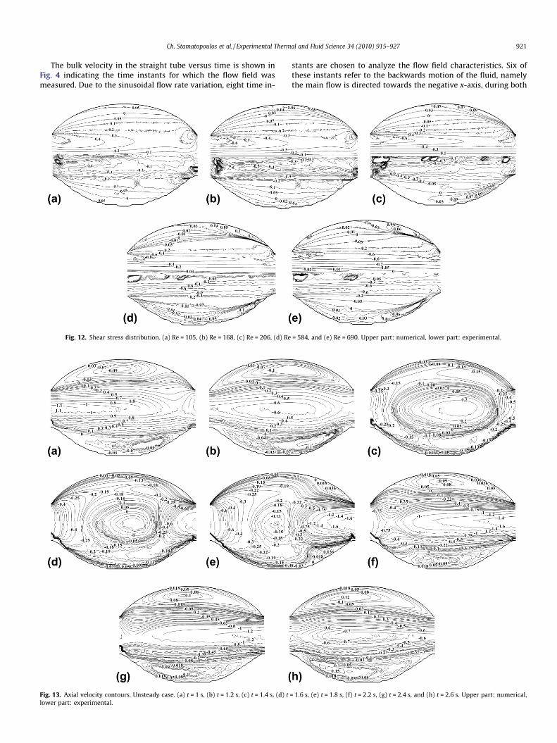
The bulk velocity in the straight tube versus time is shown inFig. 4 indicating the time instants for which the flow field wasmeasured. Due to the sinusoidal flow rate variation, eight time in-

Fig. 12. Shear stress distribution. (a) Re = 105, (b) Re = 168, (c) Re = 206, (d) Re

Fig. 13. Axial velocity contours. Unsteady case. (a) t = 1 s, (b) t = 1.2 s, (c) t = 1.4 s, (d) tlower part: experimental.

stants are chosen to analyze the flow field characteristics. Six ofthese instants refer to the backwards motion of the fluid, namelythe main flow is directed towards the negative x-axis, during both

= 584, and (e) Re = 690. Upper part: numerical, lower part: experimental.

= 1.6 s, (e) t = 1.8 s, (f) t = 2.2 s, (g) t = 2.4 s, and (h) t = 2.6 s. Upper part: numerical,

922 Ch. Stamatopoulos et al. / Experimental Thermal and Fluid Science 34 (2010) 915–927

flow acceleration (t = 1.4 s, 1.6 s, 1.8 s) and deceleration (t = 2.2 s,2.4 s, 2.6 s). Time instants t = 1.0 s and t = 1.2 s refer to the forwardmotion of the flow during its deceleration phase. During earlyacceleration (t = 1.4 s), the flow is attached to the model wall, whilethe fluid around the model central axis moves in the oppositedirection, as a continuation of the previous cycle. Consequently,

Fig. 14. Axial velocity profiles. Unsteady case. (a) t = 1 s, (b) t = 1.2 s, (c) t =

Fig. 15. Measured velocity field. Unsteady case. (a) t = 1 s, (b) t = 1.2 s, (c) t =

two stagnation points appear on the central axis, the distance ofwhich progressively is reduced, disappearing when the majorityof the fluid particles changes direction. The contours of the axialvelocity component both measured and predicted are shown inFig. 13. It has been nondimensionalized by the bulk fluid velocityof the straight tube at the peak of the flow rate. Before flow peak

1.4 s, (d) t = 1.6 s, (e) t = 1.8 s, (f) t = 2.2 s, (g) t = 2.4 s, and (h) t = 2.6 s.

1.4 s, (d) t = 1.6 s, (e) t = 1.8 s, (f) t = 2.2 s, (g) t = 2.4 s, and (h) t = 2.6 s.

Fig. 16. Wall pressure distribution. Unsteady case.

Fig. 17. Wall shear stress distribution. Unsteady case.

Ch. Stamatopoulos et al. / Experimental Thermal and Fluid Science 34 (2010) 915–927 923

the flow detaches at the proximal part of the dilatation (t = 1.6 s),forming a vortex, the extent of which increases progressively, cov-ering the major volume of the cavity at the end of the decelerationphase. As a result, the reattachment point moves along the wall,affecting both the wall shear stress and pressure distributions.Comparing the steady with the unsteady velocity fields, they exhi-bit some similarities only during the deceleration phase in a sensethat the tube dilatation is covered by a recirculation zone. How-ever, even in this phase of the cycle, in contrast to steady case,the reattachment line moves downstream instead of upstream,when the flow rate drops, namely when the Reynolds number de-creases. Furthermore, the axial velocity variation close to the mod-el axis is stronger, compared to the steady case, especially at thedistal end, as the contours of Fig. 13 clearly show. Representativeaxial velocity profiles are shown in Fig. 14, providing a gooddescription of the flow field time and space variation. A basic dif-ference between the flow at the entrance and the exit of the modelis that for the major part of the cycle the velocity profile at the exitis flat (like the case of a convergent nozzle), in contrast to the par-abolic type profiles at the inlet. During early acceleration (t = 1.4 s),it is characteristic that the velocity exhibits two maxima at boththe inlet and the exit. This is due to the fact that the flow aroundthe central axis does not change immediately direction when thebulk flow reverses. Namely, it takes some time before the flowaround the central axis changes sign along the whole length ofthe model. Therefore, during early acceleration, the major portionof the flow is directed towards the cavity, in contrast to the decel-eration phase, where this follows the central axis. The formation ofa vortex during acceleration was also detected by Yu et al. [11] fora sinusoidal flow rate waveform, employing a 2D PIV system. How-ever, in cases where physiological waveforms are used, character-ized by a faster acceleration, the vortex appears after flow peak[12,33,34], during flow deceleration. It is well documented thatimpulsively started flows behave as nonviscous for the first timesteps since it needs some finite time before the action of viscositybecomes evident [12,35–37].

The measured velocity vectors are shown in Fig. 15 for varioustime instants, displaying the formation of a vortex at the proximalpart of the model, its development and propagation. The flow field

924 Ch. Stamatopoulos et al. / Experimental Thermal and Fluid Science 34 (2010) 915–927

is shown to be axisymmetric. According to the numerical work ofJamison et al. [38] on fusiform aneurysms, the critical Re for tran-sition to three dimensionality of the flow is a function of the aneu-

Fig. 18. Normalized shear stress srx at (a)

Fig. 19. Reattachment region. Unsteady case. (a) t = 1 s, (b) t = 1.2 s,

rysm geometry and the Womersley number. More particularly,lowering the Womersley number the critical Re is reduced as well.Apparently, in our case this transition did not occur.

model entrance and (b) model exit.

(c) t = 1.6 s, (d) t = 1.8 s, (e) t = 2.2 s, (f) t = 2.4 s, and (g) t = 2.6 s.

Ch. Stamatopoulos et al. / Experimental Thermal and Fluid Science 34 (2010) 915–927 925

The wall pressure distribution along the wall of the model aswell as along the straight tubes connected to it is presented inFig. 16 in the nondimensional form p�un = (pw � pd)/Dp, where pd

is the time dependent wall static pressure 2.5 dilatation lengthsdownstream of the model and Dp is the maximum pressure differ-ence within a cycle between this station and a station 2.5 dilatationlengths upstream of the model. In the acceleration phase of the cy-cle (t = 1.4 s, 1.6 s, 1.8 s) the pressure drops linearly in the straighttubes with a rate which is proportional to flow acceleration. On theother hand, the pressure along the model is almost constant,whereas approaching its distal end it drops. It is reminded thatin the steady case quite the opposite occurs in this area with thepressure being increased due to flow reattachment. During decel-eration, there is a mild pressure recovery in the dilatation resem-bling the low Re steady cases. Practically, the pressure in thisunsteady case does not seem to vary practically within the modelin contrast to wall shear which exhibits local peaks. The same con-clusion is drawn in the numerical work of Khanafer et al. [39]where the flow of a non-Newtonian fluid in an abdominal aorticaneurysm is predicted under laminar and turbulent flow condi-tions for maximum Re of the order of 3000. Namely, they foundthat the pressure did not practically vary along the aneurysm wallwithin each cycle.

The wall shear stress, nondimensionalized by the wall shear ofthe straight tubes at the instant of the maximum flow rate, is pre-sented in Fig. 17. It exhibits extreme values at the entrance and theexit of the model, taking higher absolute values at its exit as well asduring the acceleration phase. There is also a shear peak at themoving flow reattachment line (t = 1.4 s, 1.6 s, 1.8 s) of smallerhowever value compared to the previous ones.

The distributions of shear srx at both edges of the model areshown in Fig. 18 as a function of the normalized radial distancer� (by the local bulge radius) from the model longitudinal axis.

Fig. 20. Particle paths. Unsteady case.

Fig. 18a corresponds to station x = +20 mm which is 2.5 mm up-stream of the right edge of the dilatation and Fig. 18b its symmetriccounterpart (x = �22 mm). When t > 1.2 s, bulk flow is directed to-wards negative x-axis so that Fig. 18a corresponds to the inlet ofthe model and Fig. 18b to its outlet. It is noticeable that the shearstress amplitude increases in the radial direction, being smaller atthe exit due to the blunt velocity shape at this location for the ma-jor part of the cycle. The drop of the shear close to the wall is due tothe fact that this is located inside the bulge where the flow most ofthe time is almost stagnant. This radial stress distribution is in con-trast with the remark of Yip and Yu [40] that the magnitudes of theshear stresses are uniform in the radial direction for a symmetricaneurysm, unless their flow was a plug type due to the highWomersley numbers that they examined. The central part of themodel is characterized by low and oscillating about zero wall shearstresses which according to medical evidence may energize biolog-ical mechanisms of thrombus formation [9]. In the numerical workof Khanafer et al., [39] wall shear maximum was predicted to ap-pear at the exit of an aneurysm during systole.

The motion of the formed vortex is associated with the propaga-tion of the reattachment line and consequently of the pressure andshear stress maxima. The velocity field around the reattachmentregion is presented in Fig. 19 along with the locations of pressureand wall shear maximum. It should be noted that the pressuremaximum systematically appears downstream of the reattach-ment point, like in the case of a backward facing step [41] andthe shear maximum upstream of it. During each cycle both pointstravel along the wall which is thus exposed to a cyclic loading.

Using the predicted velocity field of 30 time instants in a cycle,the particle paths of 10 massless fluid particles were computed ona Lagrangian basis, integrating the velocity field via a second-orderRunge–Kutta. The integration was performed by the commercialcode TECPLOT 360 which performs a linear interpolation between

(a) Half cycle. (b) Complete cycle.

Fig. 21. Normalized shear stress srx each particle is exposed to.

926 Ch. Stamatopoulos et al. / Experimental Thermal and Fluid Science 34 (2010) 915–927

the solution time levels. Nine of these particles were released atthe entrance of the model along a radius and the tenth at a pointin the middle of its length. Starting the integration at the instantthat the flow changes sign, the particles are released with veloci-ties which are equal to the local fluid velocities. Their paths areshown in Fig. 20 for one half of the period, namely during acceler-ation and deceleration, which correspond to 16 time instants. Dur-ing early acceleration, the particles released at the entrance of thedilatation, move towards the cavity and then they move slightlybackwards (Fig. 20a). In the next half of the period, for which thedirection of the bulk flow has changed, they exit the model follow-ing paths which are at close proximity one with the other(Fig. 20b). It is obvious that none of the released particles ap-proached the cavity walls, or it was trapped in a region close tothem. The same conclusion was drawn running several numericaltests by releasing particles at various locations. Therefore, for thisparticular flow waveform, there is no apparent evidence aboutthe residence time of the fluid particles in the cavity region whichcould be of some value from the bioengineering point of view.However, each of these particles is exposed to varying shear stres-ses during each cycle due to spatial and temporal flow variations asdepicted clearly in Fig. 21 which might be of clinical importance.Namely, it has been documented that the activation rate of plate-lets (which are responsible for thrombus formation) depends notonly on the level of shear stresses applied on them but on their dy-namic loading as well [42].

5. Conclusions

The flow field in an axisymmeric tube dilatation is examinedunder steady and time varying flow conditions, experimentallyusing 2D PIV and numerically through the commercial code FLU-ENT. The experimental data compared well with the numericalpredictions, show the same flow topology. For the steady case,where five Reynolds numbers are examined, from 105 to 690 themajor flow features are:

(a) The flow separates at the entrance of the model and it reat-taches a small distance upstream of its exit. This distancebecomes progressively smaller with increasing Re.

(b) The reattachment region is characterized by high gradientsof both wall pressure and wall shear. In the rest part of thecavity these quantities are practically unchanged. The fluidmoving upstream of the reattachment line close to the wallaccelerates for a distance and then it decelerates taking val-ues up to 15% of the inlet bulk velocity.

(c) Most of the model wall is exposed to low negative velocitieswhile the axial velocity along the longitudinal model axis ofsymmetry is almost constant, especially for the higher Re,resembling the flow field of a free jet.

(d) The shear stress srx radial gradients take high values at theexit of the model.

(e) The particle paths in the model cavity are of elliptical typeshape, the centers of which are displaced downstream withincreasing Re.

The flow field for the unsteady case (sinusoidal) with a peakRe = 272 and Womersley number 3.3 has the folowingcharacteristics:

(a) During early acceleration the major volume of the fluid isdiverted towards the walls of the model, the flow beingattached, whereas at its center it moves in the oppositedirection in continuation of the previous cycle. As a resultthe velocity at both the entrance and the exit of the aneu-rysm peaks off center and two stagnation points appear onthe central model axis which approach each other at timeprogresses, eventually disappearing.

(b) Before flow peak a vortex ring is formed at the proximal partof the model which, during deceleration, propagates down-stream, covering the whole cavity of the cavity at the endof this phase.

(c) The wall pressure varies weakly along the model and itrecovers slightly during the deceleration phase. In contrastto the steady case, it does not exhibit any extreme values.

(d) Conversely, wall shear stress takes high values close to themodel exit, being a function of the flow rate. In the majorlength of the model, it is almost constant, oscillating withsmall amplitude about a zero mean.

(e) The reattachment line moves downstream, after the forma-tion of the vortex ring, as well as the point of pressure peakwhich is always located downstream of it.

(f) The amplitude of the shear stress at the model entrance andexit increases radially.

(g) Massless particles released at various locations and timeinstants were not found to be trapped in the cavity, beingexposed to varying shear stresses which might be of clinicalimportance, like the platelet activation rate issue.

Acknowledgments

This paper is part of the 03ED244 research project, imple-mented within the framework of the ‘‘Reinforcement Programmeof Human Research Manpower” (PENED) and co-financed by Na-tional and Community Funds (20% from the Greek Ministry ofDevelopment-General Secretariat of Research and Technologyand 80% from EU – European Social Fund).

References

[1] A. Salsac, S. Sparks, J. Lasheras, Hemodynamic changes occurring during theprogressive enlargement of abdominal aortic aneurysms, Ann. Vasc. Surg. 18(1) (2004) 14–21.

[2] P.M. Brown, D.T. Zelt, B. Sobolev, The risk of rupture in untreated aneurysms:the impact of size, gender, and expansion rate, J. Vasc. Surg. 37 (2003) 280–284.

Ch. Stamatopoulos et al. / Experimental Thermal and Fluid Science 34 (2010) 915–927 927

[3] R. Limet, N. Sakalihassan, A. Albert, Determination of the expansion rate andincidence of rupture of abdominal aortic aneurysms, J. Vasc. Surg. 14 (1991)540–548.

[4] M. Fillinger, M. Raghavan, P. Marra, L. Cronenwett, E. Kennedy, In vivo analysisof mechanical stress and abdominal aortic aneurysm rupture risk, J. Vasc. Surg.36 (2002) 589–596.

[5] M. Fillinger, P. Marra, M. Raghavan, E. Kennedy, Prediction of rupture inabdominal aortic aneurysm during observation: wall stress versus diameter, J.Vasc. Surg. 37 (2003) 724–732.

[6] C. Kleinstreuer, L. Zhonghua, Analysis and computer program for rupture-riskprediction of abdominal aortic aneurysms, Biomed. Eng. Online 5 (19) (2006).

[7] A. Shaaban, A. Duerinckx, Wall shear stress and early atherosclerosis. A review,Am. J. Roentgenol. 174 (2000) 1657–1665.

[8] L. Bousel, V. Rayz, C. McColloch, A. Martin, G. Acevedo-Bolton, M. Lawton, R.Higashida, W.S. Smith, W.L. Young, D. Saloner, Aneurysm growth occurs atregion of low wall shear stress: patient-specific correlation of hemodynamicsand growth in a longitudinal study, Stroke J. Am. Heart Assoc. 39 (2008) 2997–3002.

[9] J. Lasheras, The biomechanics of arterial aneurysms, Annu. Rev. Fluid Mech. 39(2007) 293–319.

[10] D. Bluestein, L. Niu, R. Schoephoerster, M. Dewanjee, Steady flow in ananeurysm model: correlation between fluid dynamics and blood plateletdeposition, ASME J. Biomech. Eng. 118 (3) (1996) 280–286.

[11] S.C.M. Yu, W.K. Chan, B.T.H. Ng, L.P. Chua, A numerical investigation on thesteady and pulsatile flow characteristics in axisymmetric abdominal aorticaneurysm models with some experimental evaluation, J. Med. Eng. Technol. 23(26) (1999) 228–239.

[12] A. Salsac, S. Sparks, J. Chomaz, J. Lasheras, Evolution of the wall shear stressesduring the progressive enlargement of symmetric abdominal aorticaneurysms, J. Fluid Mech. 550 (2006) 19–51.

[13] V. Deplano, Y. Knapp, E. Bertrand, E. Gaillard, Flow behavior in an asymmetriccompliant experimental model for abdominal aortic aneurysm, J. Biomech. 40(11) (2007) 2406–2413.

[14] C. Asbury, J. Ruberti, E. Bluth, R. Peattie, Experimental investigation of steadyflow in rigid models of abdominal aortic aneurysms, Ann. Biomed. Eng. 23 (1)(1995) 29–39.

[15] C. Egelhoff, R. Budwig, D. Elger, T. Khraishi, K. Johansen, Model studies of theflow in abdominal aortic aneurysms during resting and exercise conditions, J.Biomech. 32 (12) (1999) 1319–1329.

[16] C. Scotti, A. Shkolnik, S. Muluk, E. Finol, Fluid–structure interaction inabdominal aortic aneurysms: effects of asymmetry and wall thickness,Biomed. Eng. Online 4 (64) (2005).

[17] Y. Papaharilaou, J. Ekaterinaris, E. Manousaki, A. Katsamouris, A decoupledfluid structure approach for estimating wall stress in abdominal aorticaneurysms, J. Biomech. 40 (2) (2007) 367–377.

[18] K. Frazer, M.-X. Li, W. Lee, W. Easson, P. Hoskins, Fluid–structure interaction inaxially symmetric models of abdominal aortic aneurysms, Proc. Inst. Mech.Eng. H 223 (2) (2009) 195–208.

[19] K. Khanafer, J. Bull, R. Berguer, Fluid–structure interaction of turbulentpulsatile flow within a flexible wall axisymmetric aortic aneurysm model,Eur. J. Mech. B – Fluids 28 (2009) 88–102.

[20] D. Ku, S. Glagov, S. Moore, C. Zarins, Flow patterns in the abdominal-aortaunder simulated postprandial and exercise conditions – an experimentalstudy, J. Vasc. Surg. 9 (2) (1989) 309–316.

[21] T. Fukushima, T. Matsuzawa, T. Homma, Visualization and finite elementanalysis of pulsatile flow in models of the abdominal aortic aneurysm,Biorheology 26 (2) (1998) 109–130.

[22] J. Moore, D. Ku, C. Zarins, S. Glagov, Pulsatile flow visualization in theabdominal aorta under differing physiological conditions – implications forincreased susceptibility to atherosclerosis, ASME J. Biomech. Eng. 114 (3)(1992) 391–397.

[23] E. Pedersen, A. Yoganathan, X. Lefebvre, Pulsatile flow visualization in a modelof the human abdominal aorta and aortic bifurcation, J. Biomech. 25 (8) (1992)935–944.

[24] F. Durst, S. Ray, B. Unsal, O. Bayoumi, The development lengths of laminar pipeand channel flows, J. Fluids Eng., ASME 127 (2005) 1154–1160.

[25] H. Xiaoyi, D. Ku, Unsteady entrance flow development in a straight tube, J.Bioeng. 116 (1994) 355–360.

[26] J. Krijger, B. Hillen, H. Hoogstraten, Pulsating entry flow in a plane channel, J.Appl. Math. Phys. (ZAMP) 42 (1991) 139–153.

[27] R. Budwig, D. Elger, H. Hooper, J. Slippy, Steady flow in abdominal aorticaneurysm models, Trans. ASME 115 (1993) 418–423.

[28] J. Ekaterinaris, C. Ioannou, A. Katsamouris, Flow dynamics in expansionscharacterizing abdominal aorta aneurysms, Ann. Vasc. Surg. 20 (2006) 351–359.

[29] E. Finol, C. Amon, Flow induced wall shear stress in abdominal aorticaneurysms: part I – steady flow hemodynamics, Comp. Meth. Biomech.Biomed. Eng. 5 (4) (2002) 309–318.

[30] M. Bonert, R. Leask, J. Butany, C. Ehier, J. Myers, K. Johnston, M. Ojha, Therelationship between wall shear stress distribution and intimal thickening inthe human abdominal aorta, Biomed. Eng. Online 2 (18) (2003).

[31] D. Ku, Blood flow in arteries, Annu. Rev. Fluid Mech. 29 (1997) 399–434.[32] C. Lentner (Ed.), Geigy Scientific Tables, Heart and Circulation, eighth ed., vol.

5, CIBA-GEIGY, 1990.[33] E. Finol, C. Amon, Flow induced wall shear stress in abdominal aortic

aneurysms: part II – pulsatile flow hemodynamics, Comput. Meth. Biomech.Biomed. Eng. 5 (4) (2002) 319–328.

[34] E. Finol, K. Keyhani, C. Amon, The effect of asymmetry in abdominal aorticaneurysms under physiologically realistic pulsatile flow conditions, J.Biomech. Eng. 125 (2003) 207–217.

[35] D. Telionis, Unsteady Viscous Flows, Springer Verlag, New York, 1981. pp80..[36] J. Anagnostopoulos, D.S. Mathioulakis, Unsteady flow field in a square tube T-

junction, J. Phys. Fluids 16 (11) (2004) 3900–3910.[37] J. Anagnostopoulos, D.S. Mathioulakis, A flow study around a time-dependent

3-D asymmetric constriction, J. Fluids Struct. 19 (2004) 49–62.[38] R. Jamison, G. Sheard, K. Ryan, A. Fouras, The validity of axisymmetric

assumptions when investigating pulsatile biological flows, ANZIAM J. 50(2009) C713–C728.

[39] K. Khanafer, J. Bull, G. Upchurch, R. Berguer, Turbulence significantly increasespressure and fluid shear stresses in an aortic aneurysm model under restingand exercise flow conditions, Ann. Vasc. Surg. 21 (2007) 67–74.

[40] T.H. Yip, S.C.M. Yu, Cyclic flow characteristics in an idealized asymmetricabdominal aortic aneurysm model, Proc. Inst. Mech. Eng. H 217 (2003) 27–39.

[41] V. Uruba, P. Jonas, O. Mazur, Control of a channel-flow behind a backward-facing step by suction/blowing, Int. J. Heat Fluid Flow 28 (2007) 665–672.

[42] M. Nobili, J. Sheriff, U. Morbiducci, A. Redaelli, D. Bluestein, Platelet activationdue to hemodynamic shear stresses: damage accumulation model andcomparison to in vitro measurements, J. ASAIO 54 (1) (2008) 64–72.