1

Experimental study of tip vortex flow from a periodically pitched airfoil section

K.B.M.Q. Zaman1, A. F. Fagan2 and M. R. Mankbadi3

NASA Glenn Research Center

Cleveland, OH 44135

Abstract An experimental investigation of a tip vortex from a NACA0012 airfoil is conducted in a low-speed wind tunnel at a chord Reynolds number of 4x104. Initially, data for a stationary airfoil held at various angles-of-

attack () are gathered. Detailed surveys are done for two cases: =10 with attached flow and =25 with

massive flow separation on the upper surface. Distributions of various properties are obtained using hot-wire anemometry. Data include mean velocity, streamwise vorticity and turbulent stresses at various streamwise locations. For all cases, the vortex core is seen to involve a mean velocity deficit. The deficit apparently

traces to the airfoil wake, part of which gets wrapped by the tip vortex. At small , the vortex is laminar

within the measurement domain. The strength of the vortex increases with increasing but undergoes a

sudden drop around 16. The drop in peak vorticity level is accompanied by transition and a sharp rise in

turbulence within the core. Data are also acquired with the airfoil pitched sinusoidally. All oscillation cases

pertain to a mean =15 while the amplitude and frequency are varied. An example of phase-averaged data

for an amplitude of ±10 and a reduced frequency of k=0.2 is discussed. All results are compared with

available data from the literature shedding further light on the complex dynamics of the tip vortex.

1. Introduction The characteristics of a tip vortex pertain to a wide variety of applications. They are of concern in tip clearance losses in turbomachinary, noise from rotorcraft and submarine propellers, safety and efficiency in aircraft traffic control as well as performance of all lifting vehicles. A strong tip vortex translates to losses in performance and therefore a reduction in its strength is sought through design considerations as well as flow control. There is a need for a deeper fundamental understanding of the associated fluid dynamics. Across various disciplines, designers stand to benefit from a better understanding of phenomena such as the formation and merger of vortex systems from the pressure and suction sides of a lifting surface, migration of velocity deficit and turbulence from the wake of the lifting body affecting subsequent behavior of the tip vortex, mean velocity deficit or excess within the vortex core as well as its life-span and stability characteristics. Flow control efforts aiming to weaken tip vortex strength can also benefit from a better understanding of the flow dynamics. Dreyer et al. [1] qualitatively explored the effect of tip leakage vortices on cavitation erosion issues relevant to turbines. For low speed flows, they incrementally decreased the gap size between the ‘runner’ and the ‘discharge ring’ until the vortex intensity reached a maximum followed by a sharp decrease. Tip clearance

1 Inlets & Nozzles Branch, AIAA Associate Fellow. 2 Optics & Photonics Branch, AIAA Associate Fellow. 3 Inlets & Nozzles Branch, AIAA member.

https://ntrs.nasa.gov/search.jsp?R=20160004766 2018-09-14T22:54:53+00:00Z

2

gap size, dictating the tip vortex strength, was also identified to be a critical parameter in cooling strategies in high pressure turbines [2]; a numerical study of flow and heat transfer in axial turbines is given in [3]. Casalino et. al. [4] studied tip vortex roll-up and its impact on airframe noise. Their analysis revealed a connection between the far-field noise and the kinematics of the two vortices generated from the lower and upper edges of the wing tip. For an aircraft, the tip vortex is responsible for induced drag and increased noise. It also dictates the safe distance needed between aircrafts in air traffic control [5]. Various flow control studies have also been carried out in order to reduce the strength of the tip vortex [2, 6].

Despite the progress achieved so far, many of the cited studies made an appeal for the need of further fundamental studies of a tip vortex. In [5], outlook for prediction as related to air traffic control is summed as, “distinct improvements in our ability to predict the motion and persistence of trailing vortices are needed before analysis is widely of value…” In connection with noise generation, authors of [4] commented, “…the role of turbulent fluctuations…and their ingestion by, and roll up into, the tip vortices needs to be investigated in more detail”. Similar comments are made in [7] in connection with tip vortex dynamics in wind turbines and rotorcrafts, as well as in [6] in connection with flow control. The present work is motivated by such calls. While more complex flow configurations are contemplated for the future, at first a simple experiment is carried out utilizing existing hardware and facilities to study the tip vortex characteristics from a rectangular airfoil section. First, a parametric study is performed while the angle of attack is varied statically. In many applications, especially with rotorcraft and some situations with turbomachinery, the effective angle-of-attack varies within the rotation cycle. This is likely to affect the tip vortex dynamics. Such effects have been explored only in a few past experiments, as cited in the following. Thus, the present study with the simple setup is extended to explore dynamic effects on the tip vortex by periodically oscillating the airfoil in

pitch. Data are acquired with the airfoil oscillated about a mean angle-of-attack of = 15 while varying the

frequency and the amplitude. A body of fundamental studies of tip vortices from rectangular wing sections (static) exists in the literature (e.g., [8-11]). A few of these are briefly reviewed here. A NACA0012 section (0.203m chord) with square tip (not rounded) was used by Devenport et. al. [8]. A four sensor hot-wire probe was used to acquire the data at Re=5.3x105. The downstream evolution of the flow was studied over 5<x/c<30; (cited x-locations are converted to current convention with origin located at one-quarter chord from the leading edge). Streamwise

vorticity (X) as well as turbulent spectra data were discussed. The issue of probe interference as well as

spatial ‘wandering’ of the vortex was addressed and both effects were inferred not to be significant within their measurement domain. Chow et. al. [9] made detailed measurements for a NACA0012 half wing section with rounded tip (1.22m chord x 0.91m span) at Re= 4.6x106. Data were acquired by a seven-hole pressure probe as well as a triple-wire hot-wire probe. The emphasis was around the tip region and the measurement domain extended downstream up to x/c=1.43. Distributions of cross-flow velocity (V2+W2)1/2and axial velocity U were presented to study the initial formation of the tip vortex. Ramaprian and Zheng [10] did similar measurements over the x/c range of 1.08-4.08, for Re = 1.8x105. They used laser-doppler velocimetry

and provided U as well as X data. Birch et. al. [11] carried out measurements with a NACA0015 as well as a

cambered airfoil; both had square tips. Their measurements at Re= 2x105 were carried out by a seven-hole

probe and distributions of U as well as X were discussed. The authors of both references [10] and [11]

3

followed up with experiments where the airfoil was oscillated periodically in pitch [12, 13]. Some of these data will be invoked and compared with during discussion of the present results.

2. Experimental Procedure

The experiment is carried out in an open-loop, low-speed wind tunnel. The test section is 50 cm high x 76 cm wide and the 16:1 contraction ratio inlet has 5 flow conditioning screens. The flow is driven by an axial fan located on the downstream end. The airfoil used has a NACA0012 profile with 7.62 cm chord and 25.4 cm span; it has a square tip with sharp edges. A picture of the wind tunnel test section is shown in Fig. 1(a). The tunnel velocity, U∞= 8 m/s, corresponds to a chord Reynolds number (Re) of 4x104. (Relative to many applications this Re, dictated by facility constraints, is low; however, Re may have only a minor influence at

large angles-of-attack () when flow separation occurs from near the leading edge. Furthermore, the low Re

flow may offer some advantage if the results are used for validation of unsteady numerical simulations). The airfoil is supported from one wall while its other end stands free in the test section. A 0.635 cm cylindrical rod attached to the airfoil passes through the wind tunnel wall and is supported outside by two bearings spaced 10 cm apart. The other end of the rod is attached to the oscillation (pitching) mechanism via a

coupling (Fig. 1b; [14]). The data are first gathered for the airfoil held stationary at various up to 35

degrees. Detailed field properties are acquired for = 10 and 25. Two crossed hot-wires, one in u-v and the other in u-w configuration and spaced 1.12 cm in z (Fig. 1c), are used to obtain all three components of mean velocity and various turbulent stresses. The data from the u-w probe are appropriately shifted to coincide with grid points covered by the u-v probe. Probe traversing mechanisms, with 0.025 mm resolution, are used under automated computer control. Gradients of the

transverse mean velocities provide streamwise vorticity (X). For all data sets, the hot-wire calibration was

checked at a fixed location in the freestream. The measured U values there were typically within 2% of U∞. Those measured values of U from the two probes were later used to normalize the respective data from each probe. The value of U∞ was monitored by a fixed Pitot-static probe with each data point during the surveys. Root-mean-square deviation of U∞ (with respect to mean) is within 0.25% for all data sets presented. Standard PC based National Instruments data system is used for data acquisition. Most of the data are based on 5 second averaging. Typical surveys on a cross-sectional plane at a fixed x took about an hour. Figure 1(c) shows a picture of the airfoil inside the test section with the two hot-wire probes downstream. Figure 1(d) shows a schematic of the airfoil. The coordinate origin is located at the tip of the airfoil and at the support axis at one-quarter-chord from the leading edge; positive-z (‘inboard’) direction is into the page. The two measurement planes marked ‘A’ and ‘B’ will be explained later with the results. The airfoil is pitched about the z-axis. All distances are nondimensionalized by the chord (c=7.62 cm) and velocities by U∞. The

frequency of oscillation (f, Hz) is nondimensionalized as k=fc/U∞. All oscillation case data are acquired

with a mean = 15 while varying the reduced frequency (k) as well as the amplitude of oscillation. While

the oscillation is done sinusoidally, the oscillation cases are denoted as 15, where is the swing

amplitude in degrees.

4

Flow visualization is accomplished by introducing a tube of smoke (approximately 15 cm diameter) from near the inlet of the tunnel and passed over the tip of the airfoil. The flowfield was illuminated by a laser-sheet. In another set of runs, global lighting was used in addition to the laser-sheet in order to obtain a global view of the flowfield associated with the tip vortex. (It is instructive to note that the smoke had to be cool with an approximate temperature the same as ambient. Initially, a generator was used that produced warm

smoke with a temperature of about 50C. It resulted in a spurious ‘mushroom’ shaped vortical structure

induced by buoyancy effects that was accentuated by the contraction section. This completely obscured the tip vortex from the airfoil.)

3. Results

Figure 2 shows flow visualization pictures of the tip vortex, obtained by a laser-sheet passing perpendicular to the flow at approximately x=3.2. The airfoil is held fixed at various angles-of-attack and the view is from upstream at an angle to the x-axis; (the camera and a small laser with optics in front, all located outside of the

test section, can be seen in Fig. 1a). The tip vortex with clockwise rotation is evident at all values of. The

vortex is laminar at small but in the range 15-20 it appears to transition to turbulence. Also, with

increasing , at first it appears to gain strength becoming the strongest around 10 but gets diffused after

transition at larger values of . At = 35 it is barely identifiable from the flow visualization pictures.

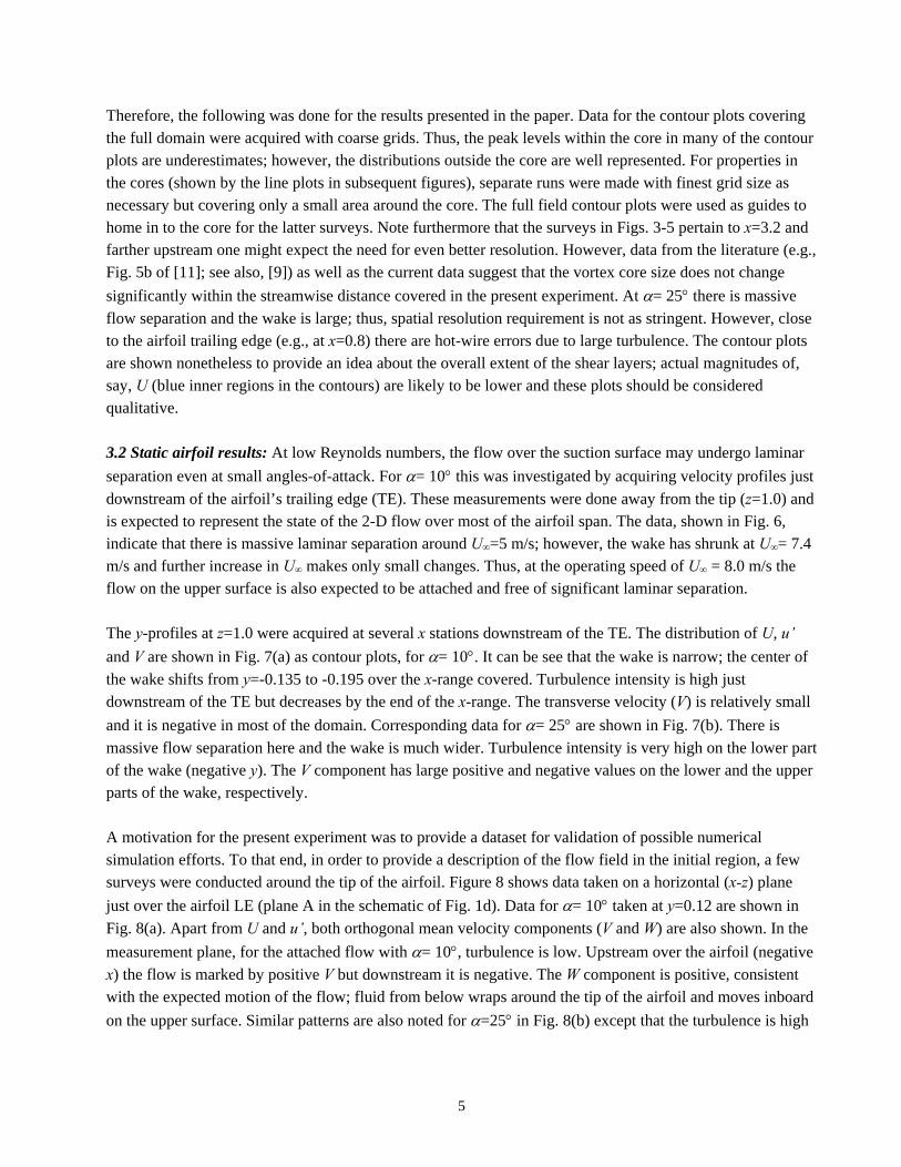
3.1 Measurement grid sensitivity: Detailed hot-wire surveys were conducted for various at x=3.2 and for

limited at various x. First, a study was conducted for measurement grid sensitivity (spatial resolution).

Figure 3(a) shows contours of mean velocity (U) and streamwise vorticity (X) for = 25 while the grid size

(same in y and z) was varied. The measurement domain was chosen after preliminary surveys to capture the core of the vortex. Note that a mean velocity deficit occurs in the core. As expected, the magnitude of the velocity deficit (i.e., U-minimum within the vortex core, denoted in the following as Ucore) and the peak in

streamwise vorticity (denoted in the following as X-peak) become less accentuated with increasing grid

size. This is shown in the graph in Fig. 3(b) from a set of similar measurements. It can be seen that with

decreasing grid size the amplitudes of Ucore and X-peak level out. Thus, for the case under consideration, a

grid size of about 0.05 was considered adequate.

Similar data for = 10 at x=3.2 are shown in Fig. 4. For this case the flow over the airfoil is likely attached

(see further discussion shortly), and thus the tip vortex is tighter in radius; note the difference in scale

between Figs. 3(a) and 4(a). Thus, the 10 case required finer spatial resolution in the measurements. The

data in Fig. 4(b) suggest that a grid size of at least 0.02 may be required to resolve the flow. However, the mean velocity profiles through the vortex core, shown in Fig. 5, demonstrate that the said grid size is adequate and further reduction in grid size does not resolve the flow any better. The smallest grid in Fig. 5 is somewhat less than the probe volume (spacing of the sensors in a given X-probe) and thus represents the best that can be done with the X-wire technique. Note that with a small grid size the acquisition time in the surveys become prohibitively large. With a fine resolution and 5 sec averages, it would take several hours to complete a survey for the full domain. This was not practical not only because of time considerations but also because of possible calibration drifts.

5

Therefore, the following was done for the results presented in the paper. Data for the contour plots covering the full domain were acquired with coarse grids. Thus, the peak levels within the core in many of the contour plots are underestimates; however, the distributions outside the core are well represented. For properties in the cores (shown by the line plots in subsequent figures), separate runs were made with finest grid size as necessary but covering only a small area around the core. The full field contour plots were used as guides to home in to the core for the latter surveys. Note furthermore that the surveys in Figs. 3-5 pertain to x=3.2 and farther upstream one might expect the need for even better resolution. However, data from the literature (e.g., Fig. 5b of [11]; see also, [9]) as well as the current data suggest that the vortex core size does not change

significantly within the streamwise distance covered in the present experiment. At = 25 there is massive

flow separation and the wake is large; thus, spatial resolution requirement is not as stringent. However, close to the airfoil trailing edge (e.g., at x=0.8) there are hot-wire errors due to large turbulence. The contour plots are shown nonetheless to provide an idea about the overall extent of the shear layers; actual magnitudes of, say, U (blue inner regions in the contours) are likely to be lower and these plots should be considered qualitative. 3.2 Static airfoil results: At low Reynolds numbers, the flow over the suction surface may undergo laminar

separation even at small angles-of-attack. For = 10 this was investigated by acquiring velocity profiles just

downstream of the airfoil’s trailing edge (TE). These measurements were done away from the tip (z=1.0) and is expected to represent the state of the 2-D flow over most of the airfoil span. The data, shown in Fig. 6, indicate that there is massive laminar separation around U∞=5 m/s; however, the wake has shrunk at U∞= 7.4 m/s and further increase in U∞ makes only small changes. Thus, at the operating speed of U∞ = 8.0 m/s the flow on the upper surface is also expected to be attached and free of significant laminar separation. The y-profiles at z=1.0 were acquired at several x stations downstream of the TE. The distribution of U, u’

and V are shown in Fig. 7(a) as contour plots, for = 10. It can be see that the wake is narrow; the center of

the wake shifts from y=-0.135 to -0.195 over the x-range covered. Turbulence intensity is high just downstream of the TE but decreases by the end of the x-range. The transverse velocity (V) is relatively small

and it is negative in most of the domain. Corresponding data for = 25 are shown in Fig. 7(b). There is

massive flow separation here and the wake is much wider. Turbulence intensity is very high on the lower part of the wake (negative y). The V component has large positive and negative values on the lower and the upper parts of the wake, respectively. A motivation for the present experiment was to provide a dataset for validation of possible numerical simulation efforts. To that end, in order to provide a description of the flow field in the initial region, a few surveys were conducted around the tip of the airfoil. Figure 8 shows data taken on a horizontal (x-z) plane

just over the airfoil LE (plane A in the schematic of Fig. 1d). Data for = 10 taken at y=0.12 are shown in

Fig. 8(a). Apart from U and u’, both orthogonal mean velocity components (V and W) are also shown. In the

measurement plane, for the attached flow with = 10, turbulence is low. Upstream over the airfoil (negative

x) the flow is marked by positive V but downstream it is negative. The W component is positive, consistent with the expected motion of the flow; fluid from below wraps around the tip of the airfoil and moves inboard

on the upper surface. Similar patterns are also noted for =25 in Fig. 8(b) except that the turbulence is high

6

in the measurement plane. The survey plane for the latter case is somewhat higher (y=0.15) in order to clear the upper edges of the leading edge. Distributions of U, u’ and V, on a vertical (x-y) plane and to the side of the airfoil tip (plane B in the schematic of Fig. 1d) are shown in Fig. 9. The measurement plane is at z=-0.08 and the data are shown in

Figs. 9(a) and (b) for = 10 and 25, respectively. Due to the configuration of the probes (see §2), only the

u-v probe could be brought close to the airfoil tip and the W component could not be acquired at the same plane. (The u-w probe was separated from u-v probe by 0.147c. This is also why the z-extent of the

measurement domain for quantities like W and X, coincident with u-v probe domain, is shorter). Again,

turbulence is low for = 10, while it is large for = 25. The V component is mostly positive (directed

upward) at the measurement plane for both cases.

Detailed cross-sectional distributions of various properties at downstream locations are shown next. Only U,

u’ and X data are discussed for brevity. Data at x=3.2 are shown in Fig. 10 for five values of. Distributions

of the three properties are shown in the three rows, as indicated in the caption. All three identify the location

of the tip vortex. It is represented most unambiguously by the distribution of X. An inspection of the legends

of the X data indicate that vorticity in the core attains maximum amplitude in the -range of 10-15 (recall

that the peak levels in the contour plots may be underestimates and representative values are discussed shortly). Comparison with the u’ data shows that the vortex core is characterized by high turbulence

intensity. The intensity jumps up significantly from =15 to 20, indicating transition to turbulent state.

Comparison of U and X data shows that the core of the vortex is associated with a velocity deficit at all

values of . Thus, the tip vortex core is seen to involve a ‘wake-like’ profile in the present case. Note that at

smaller , there are regions of excess velocity at upper and lower edges of the vortex core. These trends are

discussed further in the following.

The vortex core region was probed with fine probe resolution. Based on such measurements, X-peak and

Ucore values are shown in Fig. 11(a) as a function of . It can be seen that X -peak at first increases with

increasing , reaches a maximum around =10, stays about the same for a range, and then abruptly drops

around 16°. The initial increase in X -peak is expected as lift increases with . The tip vortex strength

follows lift produced by the airfoil. The drop-off around 16° is likely to be due to the onset of stall with sudden decrease in lift; this is also tied to transition of the vortex core to turbulence. The value of Ucore exhibits an initial drop then stays about the same (0.7-0.8) until dropping off at the onset of stall (around

=16). The velocity deficit in the core attains as low a value as Ucore = 0.37U∞ just after stall but then

increases somewhat with further increase in . Peak turbulence intensity in the vicinity of the vortex core is

shown separately in Fig. 11(b). The most conspicuous feature is the rapid rise in the intensity around =16. The level reaches a maximum of 0.22U∞ but then gradually drops off with further increase in .

The value of X-peak of about 23 at =10 (Fig. 11a) compares reasonably well with that (about 26)

reported in [11] for a NACA0015 wing at same incidence (their Fig. 5d). Comparable values were also

reported in [10] for a NACA0012 airfoil at =10 (their Fig. 3). Similar data presented in [8] (their Fig. 8c)

appears to indicate a much lower value for X-peak. While detailed surveys were conducted in the work of

7

[9], unfortunately, X data were not presented. It is interesting that in [11] significantly higher X-peak value

(about 40) was reported with a different (cambered) airfoil. These comparisons suggest that the peak vorticity may be sensitive to detailed geometry of the airfoil tip and its overall lift characteristics. Similar comparisons of the velocity deficit in the core (Ucore) are discussed in the following.

The streamwise evolution of the flowfield for =10 is presented in Fig. 12. U, u’ and X data are shown

similarly as in Fig. 10, for five x-stations. As noted before, comparison of U- and X-distributions shows that

there are regions of high U both above and below the vortex core at all stations. However, the core location is marked by a region of low U. At the upstream-most location it can be seen that the velocity deficit in the core is connected with the region of velocity defect from the wake of the airfoil; (the latter is seen as the band of horizontal contours in blue). Further downstream, the vortex core moves to the right (inboard) while the wake of the airfoil recedes farther inboard. The turbulence intensity in the core is relatively high at locations close to the airfoil (x=0.8) but has diminished substantially farther downstream. The high intensity up close to the TE also appears to be due to ingestion of airfoil wake fluid into the core of the tip vortex.

Similar data for =25 are shown in Fig. 13. At x=0.8, the vortex appears ill-defined. However, by x=1.6 the

tip vortex has taken clear shape. At this , peak vorticity is much smaller while turbulence intensity is much

larger, relative to the =10 case. Overall, the X distribution has an oblong shape that gently rotates

clockwise with increasing downstream distance. The U-distribution exhibits a similar overall trend as

described for the =10° case. From the two sets of data shown in Figs 12 and 13, it is apparent that the

velocity deficit region within the vortex core has its origin in the wake from the airfoil. Part of the wake is pulled off and gets wrapped into the vortex core. The deficit persists at the farthest downstream location covered in the experiment.

The variations of X -peak and Ucore with x for =10° and 25° are shown in Figs. 14(a) and (b), respectively,

in a similar manner as in Fig. 11(a). For =10°, X -peak initially increases reaching a maximum around

x=1.75 and then decreases with farther increase in x. This trend is somewhat different from that reported in [11] where the level practically remained a constant over the x-range covered (see earlier discussion of Fig.

11). The trend of Ucore is not well-defined but it generally follows that of the X –peak. At =25° (Fig. 14b),

on the other hand, a clear trend has emerged for Ucore. As the separated flow from the wake of the airfoil is ingested within the vortex, Ucore is very low initially. Farther downstream it increases and levels off at a value

of about 0.6. The amplitude of X -peak for this case is seen to be roughly five times lower compared to that

for the =10° case, and stays within the range of 4.5-5.5.

The axial flow (U-distribution) within the tip vortex has a “rich behavior”; quoting from [5] in connection with review of airplane wing tip vortex data, “it has surprised many of us that the velocity relative to the

atmosphere may be directed towards the airplane but also away from it”. For =10°, Chow et al. [9] reported

a large excess velocity, up to 1.77U∞. On the other hand, a velocity deficit is reported in [10] (0.68-0.78U∞; their Fig. 2). In [11] a velocity excess is reported for the cambered airfoil (1.1-1.3U∞) but just about 1.0U∞ for the NACA0015 airfoil (their Fig. 5e). A velocity deficit is also reported in [8] (their Fig. 20). Thus, it appears to be an issue researchers have hardly agreed on. Clearly, the airfoil geometry and operating conditions must play a role. In the present case at the low Re and for the NACA0012 airfoil with square tip,

8

the core is always seen to involve a velocity deficit. Tracing the evolution of the core, it is apparent that the deficit has its origin in the wake from the airfoil. Part of the wake is ingested by the tip vortex that manifests as the deficit. After an initial decay in magnitude, it persists practically unabated as far downstream as covered in the experiment.

The excess velocities (U>1) seen above and below the vortex core for the =10° case (Fig. 12) seem to have

their origin in the flow from near the leading edge. Past the stagnation point the flow accelerates as it passes over the LE. Thus, there is a region over the LE where U>1; (a classic example is shocks over the wing even when an airplane flies subsonically). Similarly, there is also a region of excess U underneath the LE even though its magnitude is not as high as seen over the LE. It is apparent that these high velocity regions persist downstream and manifest as the regions of excess U above and below the tip vortex core. A similar effect

also occurs at =25°, however, the flow acceleration around the LE is diminished due to massive separation.

Regions of higher velocities can indeed be detected in Fig. 13 especially above the tip vortex even though the magnitudes are barely above unity.

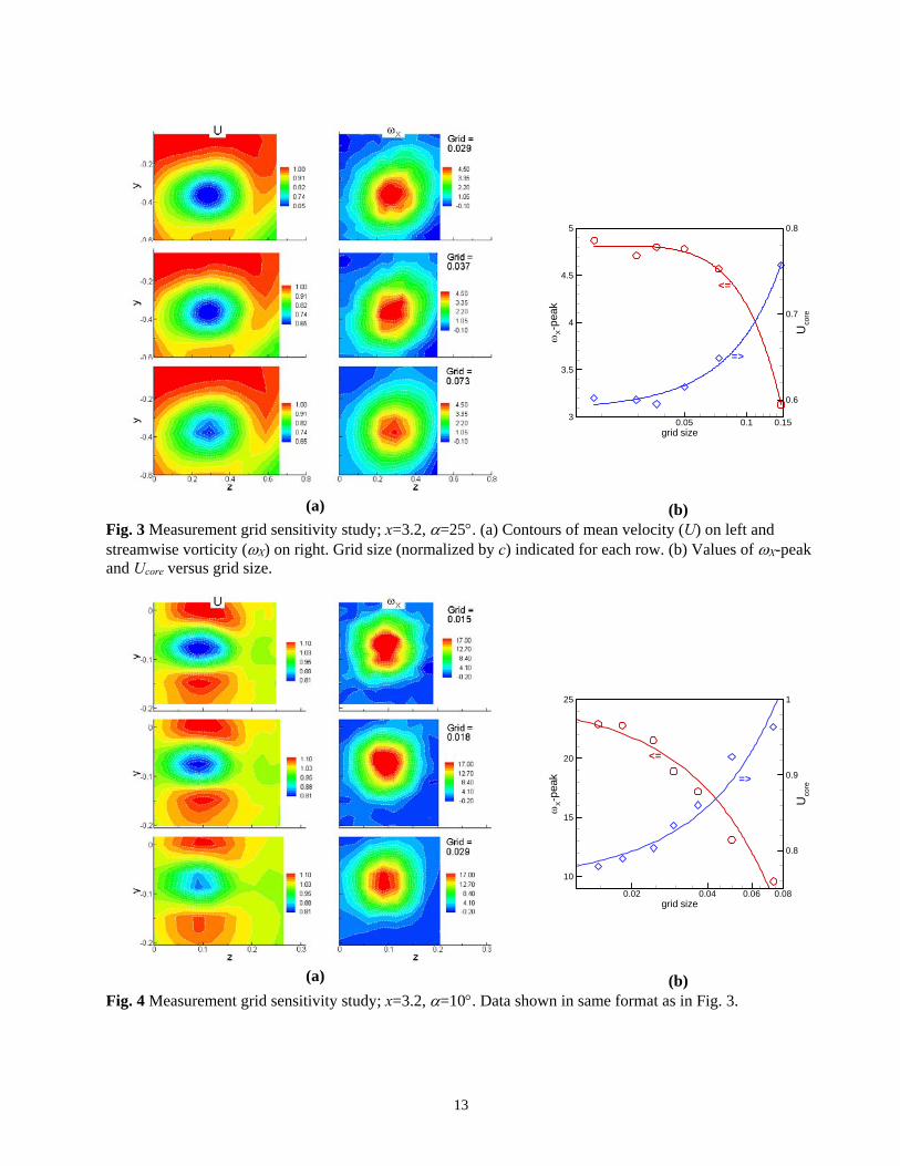
The trajectories of the vortex core for =10° and 25° are documented in Fig. 15. The core location data on x-

z and x-y planes are shown in (a) and (b), respectively. The movement of the core for =25° is more

pronounced. With increasing x, the core moves inboard (positive z) and downward (negative y). A similar

movement is also noted for =10° albeit the magnitudes are smaller. Similar data could be found in [10]. At

=10° and with increasing x, an inboard movement of the core in z was reported. However, there was a clear

“rise” in y (their Fig. 5); the magnitudes were also relatively large compared to the present =10° data. Once

again, reasons for the different behavior in the y-direction remain from being clear but are likely due to differences in geometric and operating conditions. 3.3 Oscillating airfoil results: Limited data were acquired with the airfoil pitched sinusoidally about the z-

axis with a mean =15. Nondimensional oscillation frequencies (k=fc/U∞) of 0.08, 0.165, 0.2 and 0.33

were covered. Dynamic stall from a 2-D flow (airfoil spanning the entire width of the test section) was studied before for comparable range of k in the same facility [14]. The highest k with the given U∞ (8 m/s) corresponded to a physical frequency of 10.2 Hz. This was the limit beyond which structural issues might

become a concern. Amplitudes of ±2.5, ±5, ±10 and ±15 were covered. For brevity, data only for an

example of the cases is presented in the following.

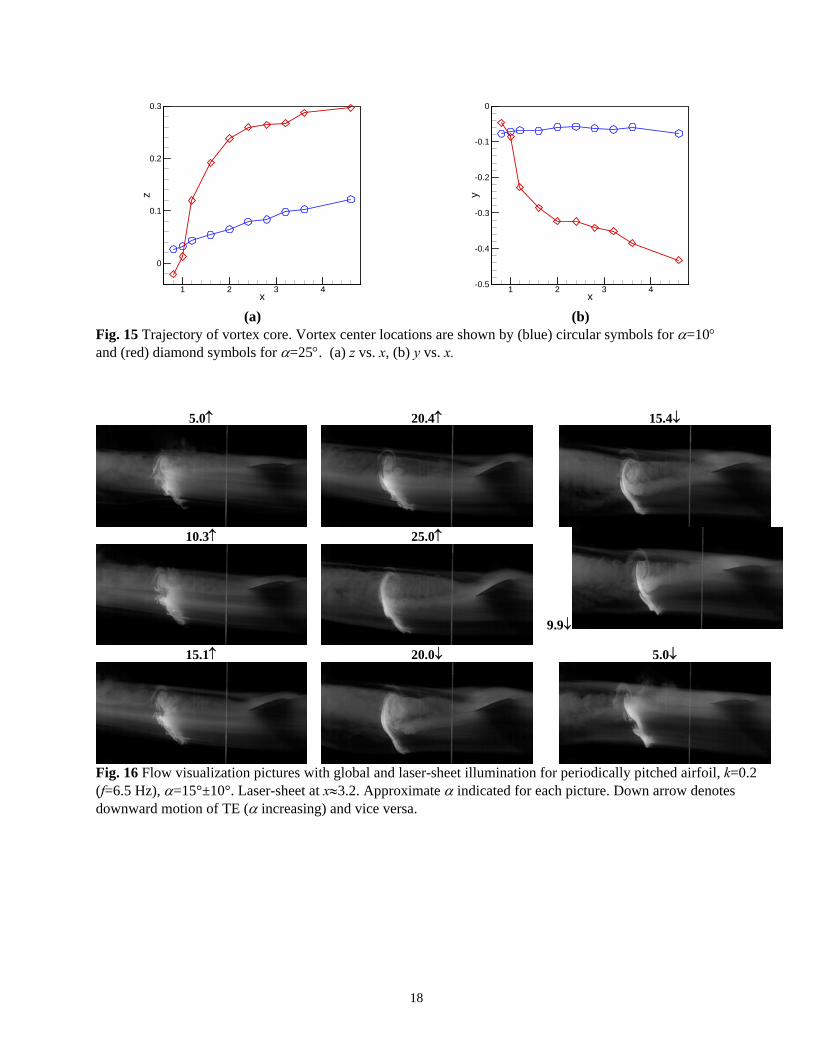
Figure 16 shows flow visualization pictures from a movie sequence for oscillation at k=0.2 (6.5 Hz;

=15±10). The pictures correspond to certain values of as indicated, the arrows denoting the direction of

motion. The frames are chosen such that there are pairs at same but with opposite direction of motion. The

framing rate was 500/sec and the laser-sheet location is at x=3.2. Additional flood lighting is used in order to obtain a global view. The pitching motion of the airfoil with varying frames can be seen and the laser-sheet illuminated cross-section bears resemblance to the stationary airfoil data shown in Fig. 2. In some of the

pictures (especially at large ) a twisting motion of the flow from the upper and lower surfaces of the airfoil

can be detected. Bands of smoke twist clockwise with increasing downstream distance consistent with the

sense of the tip vortex. Comparison of the pictures at same but different direction of motion reveals that the

9

tip vortex is somewhat more organized during the pitch-up motion ( decreasing) compared to the pitch-

down ( increasing) case. This is discussed further in the following.

For same conditions of Fig. 16 (k=0.2 and =15±10), phase-averaged velocity and vorticity data are

shown in Figs. 17 and 18, respectively. As with the flow visualization these data are also shown over a

complete period; pairs of plots are chosen at given with opposite directions of motion, as indicated.

Comparing these with corresponding data for stationary airfoil (Fig. 10), some dynamic effects are evident. As noted with the flow visualization data, there is a difference at same angle but with different direction of motion. The vortex structure is seen to be better organized during pitch-up. Compare for example, the

distributions at 16.7° and 16.7° cases; the vortex structure is faint and almost unrecognizable in the latter

case. This difference obviously traces to the flow over the airfoil which can be quite different between pitch-up and pitch-down states of the oscillation. The phenomenon of ‘dynamic stall’ takes place. During part of the oscillation the flow remains attached resulting in a coherent tip vortex (well organized) whereas at other times the flow is separated resulting is a weak and diffused tip vortex. Difference between pitch-up and pitch-down states in the cycle has also been noted in both [12] and [13] that reported results for periodically oscillated airfoil. In [12] measurements were carried out with the airfoil

oscillated at k=0.1 and =10±5, while in [13] data were reported for k=0.18 and =14±6. Small

differences in pitch-up versus pitch-down motions can be seen in the data of [13] (their Fig. 5); the vortex core appears to be better organized during the pitch-up motion. However, in [12] a better organized vortex structure is clearly seen during pitch-down (their Fig. 4), in contrast to the current observation. It appears that this opposite trend is simply a matter of phase lag between events over the airfoil and that noted at the measurement station. Whether the vortex is seen more organized during pitch-up or pitch-down depends on the distance of the observation location, the phase-speed as well as the oscillation frequency. This effect is further illustrated with the flow visualization pictures in Fig. 19. Pairs of pictures similar to those in Fig. 16

are presented for two other values of k. For each k, data are shown for two different . At the lower

frequency (k=0.08 in (a)), the vortex is more organized during pitch-down (opposite to that seen in Fig. 16). At the higher frequency (k=0.33 in (b)), the patterns are quite different between the two directions of motion; a clearer tip vortex might be visible during the pitch-up.

Returning to Figs. 17 and 18, note that the time-averaged data under the oscillation (‘time-ave 1510’) is also

shown. This would be the distribution if all the phase-locked distributions were summed and averaged. In

addition, the stationary case data at the mean (‘time-ave 150’) are also shown for comparison. A distinct

tip vortex structure is seen even under the oscillation, in the time-averaged flow. The velocity deficit is more pronounced relative to the stationary case; it is as if this distribution is weighted more by conditions at larger

values. The oscillation has resulted in a lower X –peak relative to the stationary case. As indicated before,

detailed phase-averaged data have also been acquired for other oscillation frequencies and amplitudes. These are not included here for brevity. A NASA Technical Memorandum (TM) is planned for the future that will include a selected few of those cases as well as all data covered in this paper, with accompanying digital data for easy retrieval. It is hoped that these experimental results will be useful in future numerical simulation efforts. Further experimental studies in the future are also contemplated to address factors dictating the

10

complex behavior such as noted with regards to the velocity deficit in the core, as well as to study tip vortex characteristics with models simulating more complex flows.

4. Conclusions

The main inferences are enumerated as follows. (1) Streamwise vorticity (X) is a superior descriptor of the

tip vortex although mean velocity or turbulence intensity also identifies its location and overall shape. (2) For

the present conditions, the vortex is laminar until about =16° but becomes turbulent at higher. The

transition is accompanied by a sharp rise in the turbulence intensity in the vortex core, while both peak vorticity and the axial mean velocity within the core go through sharp drops in magnitudes. (3) With

increasing , peak vorticity within the core reaches a maximum at about =10, stays constant over a range,

and then drops off around =16 when transition occurs. (4) For all instances examined, the vortex core is

characterized by a mean velocity deficit (i.e., a ‘wake-like’ rather than a ‘jet-like’ profile). (5) With periodic

pitching oscillation, data at x=3.2 are documented. The flow-field at a given exhibits large differences

between pitch-up and pitch-down motions within the cycle. Similar observations were made in two prior works reported in the literature. Whether the tip vortex structure is seen more organized during pitch-up or pitch-down depends on the distance of the measurement station, phase speed, as well as frequency of oscillation.

Acknowledgement: Thanks are due to Ms. Michelle Clem for help with the flow visualization experiment. Support from the ‘Transformational Tools and Technologies’ Project of NASA’s Advanced Air Vehicles Program is gratefully acknowledged.

References: 1. Dreyer, M., Decaix, J., Munch-Alligne, C. and Farhat, M., “Mind the gap-tip leakage vortex in axial

turbines,” IOP Conf. Series: Earth and Environmental Science, 22, doi: 10.1088/1755-1315/22/5/052023, 2014.

2. Zhou, C. and Hodson, H., “The Tip Leakage Flow of an Unshrouded High Pressure Turbine Blade with Tip Cooling.” J. of Turbomachinery, ASME, 133 / 041028-1, Oct, 2011.

3. Ameri, A.A. and Rigby, D.L., “Effects of tip clearance and casing recess on heat transfer and stage efficiency in axial turbines”, J. Turbomachinery, 121 (4), pp. 683-693, doi: 10.1115/1.2836720, 1999.

4. Casalino, D., Hazir, A., Fares, E., Duda, B. , and Khorrami, M.R., “On the Connection between Flap Side-Edge Noise and Tip Vortex Dynamic.”, 21st AIAA/CEAS Aeroacoustics Conf., AIAA paper 2015-2292, 2015.

5. Spalart, P.R., “Airplane trailing vortices”, Ann. Rev. Fluid Mech., 30, pp. 107-138, 1998. 6. Margaris, P. and Gursul, I., “Vortex topology of wing tip blowing.” Aerospace Science and Technology,

14, pp. 143–160, 2010. 7. Ivanell, S., Leweke, T., Sarmast, S., Quaranta, H.U., Mikkelsen, R.F. and Sorensen, J.N. “Comparison

between experiments and Large-Eddy Simulations of tip spiral structure and geometry.” J. of Physics: Conf. Series 625, 012018, 2015.

8. Devenport, W.J., Rife, M.C., Liapis, S.I. and Follin, G.J., “The structure and development of a wing-tip vortex”, J. Fluid Mech., 312, pp. 67-106, 1996.

11

9. Chow, J.S., Zilliac, G.G. and Bradshaw, P., “Mean and turbulence measurements in the near field of a wingtip vortex”, AIAA J., 35, No. 10, pp. 1561-1567, 1997.

10. Ramaprian, B.R. and Zheng, Y., “Measurement in rollup region of the tip vortex from a rectangular wing”, AIAA J., 35, No. 12, pp. 1837-1843, 1997.

11. Birch, D., Lee, T., Mokhtarian, F. and Kafyeke, F., “Structure and induced drag of a tip vortex”, J. of Aircraft, 41, No. 5, pp. 1138-1145, 2004.

12. Ramaprian, B.R. and Zheng, Y., “Near field of the tip vortex behind an oscillating rectangular wing”, AIAA J., 36, No. 7, pp. 1837-1263-1269, 1998.

13. Birch, D. and Lee, T., “Investigation of the near-field tip vortex behind an oscillating wing”, J. Fluid Mech., 544, pp. 201-241, 2005.

14. Panda, J. and Zaman, K.B.M.Q., "Experimental investigation of the flowfield of an oscillating airfoil and estimation of lift from wake surveys", J. Fluid Mech., 265, pp. 65-95, 1994.

12

(a)

(b)

(c)

(d)

Fig. 1 Experimental facility. (a) Wind tunnel setup for flow visualization, (b) airfoil oscillation mechanism, (c) airfoil inside test section with two crossed hotwire probes downstream, (d) Sketch of airfoil with co-ordinate system.

=5°

=10°

=15°

=20°

=25°

=35°

Fig. 2 Laser-sheet illuminated smoke streaks showing cross-section of tip vortex at x3.2, for airfoil held fixed at different angles-of-attack ().

13

(a)

grid size

X-p

eak

Uco

re

0.05 0.1 0.153

3.5

4

4.5

5

0.6

0.7

0.8

<=

=>

(b) Fig. 3 Measurement grid sensitivity study; x=3.2, =25. (a) Contours of mean velocity (U) on left and streamwise vorticity (X) on right. Grid size (normalized by c) indicated for each row. (b) Values of X-peak and Ucore versus grid size.

(a)

grid size

X-p

eak

Uco

re

0.02 0.04 0.06 0.08

10

15

20

25

0.8

0.9

1

<=

=>

(b) Fig. 4 Measurement grid sensitivity study; x=3.2, =10. Data shown in same format as in Fig. 3.

14

z

U

-0.1 0 0.1 0.2

0.8

0.85

0.9

0.95

1

1.05

z=0.0093z=0.0133z=0.0183

y

U

-0.2 -0.1 0 0.1 0.20.2

0.4

0.6

0.8

1

1.2

U= 4.45U= 5.93U= 7.42U= 8.12

Fig. 5 U(z) profiles through vortex core with varying z-step (z); x=3.2, y=-0.07, =10.

Fig. 6 U(y) profiles just downstream of TE (x=0.8) and away from tip of the airfoil (z=1.0) for different freestream velocities (U , m/s); =10.

(a)

(b)

Fig. 7 Wake characteristics at z=1.0; distributions of U, u’ and V on y-x plane. (a) =10°, (b) =25°.

(a)

(b)

Fig. 8 Distributions of U, u’ and V on a horizontal (x-z) plane just above the LE (plane A in Fig. 1d): (a) =10°, y=0.12, (b) =25°, y=0.15.

15

(a)

(b)

Fig. 9 Distributions of U, u’, and V on a vertical (y-x) plane on the side of airfoil tip (plane B in Fig. 1d) at z=-0.08. (a) =10°, (b) =25°.

Fig. 10 Distributions of U, u’ and X on cross-sectional (y-z) plane at x=3.2 for different. Contours of U, u’ and X are shown in top, middle and bottom rows, respectively.

16

(deg.)

X-p

eak

Uco

re

0 10 20 300

10

20

30

40

50

-0.2

0

0.2

0.4

0.6

0.8

1

=>

<=

(a)

(deg.)

u' co

re

0 10 20 300

0.05

0.1

0.15

0.2

0.25

(b)

Fig. 11 Peak values (within y-z field at x=3.2) vs. . (a) X-peak and Ucore, (b) u’core.

Fig. 12 Distributions of U, u’ and X on cross-sectional (y-z) plane at different x; =10. Contours of U, u’ and X are shown in top, middle and bottom rows, respectively.

17

Fig. 13 Distributions of U, u’ and X on cross-sectional (y-z) plane at different x; =25. Contours of U, u’ and X are shown in top, middle and bottom rows, respectively.

x

X-p

eak

Uco

re

1 2 3 4 5

20

25

30

35

0.7

0.8=>

<=

(a)

x

X-p

eak

Uco

re

1 2 3 4 53

4

5

6

7

8

9

10

0

0.2

0.4

0.6

=>

<=

(b)

Fig. 14 Values of X-peak and Ucore in the vortex core as a function of x: (a) =10, (b) =25.

18

x

z

1 2 3 4

0

0.1

0.2

0.3

(a)

x

y

1 2 3 4-0.5

-0.4

-0.3

-0.2

-0.1

0

(b)

Fig. 15 Trajectory of vortex core. Vortex center locations are shown by (blue) circular symbols for =10 and (red) diamond symbols for =25. (a) z vs. x, (b) y vs. x.

5.0

20.4 15.4

10.3

25.0

9.9

15.1

20.0 5.0

Fig. 16 Flow visualization pictures with global and laser-sheet illumination for periodically pitched airfoil, k=0.2 (f=6.5 Hz), =15°±10°. Laser-sheet at x3.2. Approximate indicated for each picture. Down arrow denotes downward motion of TE ( increasing) and vice versa.

19

Fig. 17 Phase-averaged U distributions for periodically pitched airfoil, k=0.2 (f=6.5 Hz), =15°±10°. Data shown for every other phase (out of 19 over a period). Value of with direction of TE motion (see Fig. 16 caption for definition) is indicated at all phases. Also shown are time-averaged data for the pitching case and for stationary case at mean on right column.

20

Fig. 18 Phase-averaged X distributions for periodically pitched airfoil, k=0.2 (f=6.5 Hz), =15°±10°. Data shown similarly as in Fig. 17.

21

(a)

9.9

20.0

10.1

20.0

Fig. 17(a)

(b) 10.1

19.9

9.6

20.5

Fig. 19 Flow visualization pictures at x=3.2 similar to those in Fig. 16, =15°±10°. (a) k=0.08 (f=2.6 Hz), (b) k=0.33 (f=10.2 Hz).