EXPERIMENTAL MODAL ANALYSIS vibration is a combination of both forced and resonant vibration. Forced...

CSI Reliability Week, Orlando, FL October, 1999

of 12

EXPERIMENTAL MODAL ANALYSIS By

Brian J. Schwarz & Mark H. Richardson Vibrant Technology, Inc.

Jamestown, California 95327

ABSTRACT

Experimental modal analysis has grown steadily in popu-larity since the advent of the digital FFT spectrum analyzer in the early 1970’s. Today, impact testing (or bump testing) has become widespread as a fast and economical means of finding the modes of vibration of a machine or structure.

In this paper, we review all of the main topics associated with experimental modal analysis (or modal testing), in-cluding making FRF measurements with a FFT analyzer, modal excitation techniques, and modal parameter estima-tion from a set of FRFs (curve fitting).

INTRODUCTION

Modes are used as a simple and efficient means of character-izing resonant vibration. The majority of structures can be made to resonate. That is, under the proper conditions, a structure can be made to vibrate with excessive, sustained, oscillatory motion.

Resonant vibration is caused by an interaction between the inertial and elastic properties of the materials within a struc-ture. Resonant vibration is often the cause of, or at least a contributing factor to many of the vibration related problems that occur in structures and operating machinery.

To better understand any structural vibration problem, the resonances of a structure need to be identified and quantified. A common way of doing this is to define the structure’s mo-dal parameters.

TWO TYPES OF VIBRATION

All vibration is a combination of both forced and resonant vibration. Forced vibration can be due to,

• Internally generated forces. • Unbalances. • External loads. • Ambient excitation.

Resonant vibration occurs when one or more of the reso-nances or natural modes of vibration of a machine or struc-ture is excited. Resonant vibration typically amplifies the vibration response far beyond the level deflection, stress, and strain caused by static loading.

What are Modes? Modes (or resonances) are inherent properties of a structure. Resonances are determined by the material properties (mass, stiffness, and damping properties), and boundary conditions of the structure. Each mode is defined by a natural (modal or resonant) frequency, modal damping, and a mode shape. If either the material properties or the boundary conditions of a structure change, its modes will change. For instance, if mass is added to a vertical pump, it will vibrate differently because its modes have changed.

At or near the natural frequency of a mode, the overall vibra-tion shape (operating deflection shape) of a machine or struc-ture will tend to be dominated by the mode shape of the re-sonance.

What is an Operating Deflection Shape? An operating deflection shape (ODS) is defined as any forced motion of two or more points on a structure. Specify-ing the motion of two or more points defines a shape. Stated differently, a shape is the motion of one point relative to all others. Motion is a vector quantity, which means that it has both a location and a direction associated with it. Motion at a point in a direction is also called a Degree Of Freedom, or DOF.

“All experimental modal parameters are obtained from measured ODS’s.”

That is, experimental modal parameters are obtained by arti-ficially exciting a machine or structure, measuring its operat-ing deflection shapes (motion at two or more DOFs), and post-processing the vibration data.

Figure 1. Frequency Domain ODS From a Set of FRFs


of 12

Figure 1 shows an ODS being displayed from a set of FRF measurements with the cursor located at a resonance peak. In this case, the ODS is being dominated by a mode and there-fore is a close approximation to the mode shape.

Two Kinds of Modes Modes are further characterized as either rigid body or flexi-ble body modes. All structures can have up to six rigid body modes, three translational modes and three rotational modes. If the structure merely bounces on some soft springs, its mo-tion approximates a rigid body mode.

Figure 2. Flexible Body Modes.

Many vibration problems are caused, or at least amplified by the excitation of one or more flexible body modes. Figure 2 shows some of the common fundamental (low frequency) modes of a plate. The fundamental modes are given names like those shown in Figure 2. The higher frequency mode shapes are usually more complex in appearance, and there-fore don’t have common names.

FRF MEASUREMENTS

The Frequency Response Function (FRF) is a fundamental measurement that isolates the inherent dynamic properties of a mechanical structure. Experimental modal parameters (fre-quency, damping, and mode shape) are also obtained from a set of FRF measurements.

The FRF describes the input-output relationship between two points on a structure as a function of frequency, as shown in Figure 3. Since both force and motion are vector quantities, they have directions associated with them. Therefore, an FRF is actually defined between a single input DOF (point & direction), and a single output DOF.

An FRF is a measure of how much displacement, velocity, or acceleration response a structure has at an output DOF, per unit of excitation force at an input DOF.

Figure 3 also indicates that an FRF is defined as the ratio of the Fourier transform of an output response ( X(ω) ) di-vided by the Fourier transform of the input force ( F(ω) ) that caused the output.

Figure 3. Block Diagram of an FRF.

Depending on whether the response motion is measured as displacement, velocity, or acceleration, the FRF and its in-verse can have a variety of names,

• Compliance ó (displacement / force) • Mobility ó (velocity / force) • Inertance or Receptance ó (acceleration / force) • Dynamic Stiffness ó (1 / Compliance) • Impedance ó (1 / Mobility) • Dynamic Mass ó (1 / Inertance)

An FRF is a complex valued function of frequency that is displayed in various formats, as shown in Figure 4.

Figure 4. Alternate Formats of the FRF.

VIBRATION IS EASIER TO UNDERSTAND IN TERMS OF MODES

Figure 5 points out another reason why vibration is easier to understand in terms of modes of vibration. It is a plot of the Log Magnitude of an FRF measurement (the solid curve), but several resonance curves are also plotted as dotted lines be-


of 12

low the FRF magnitude. Each of these resonance curves is the structural response due to a single mode of vibration.

The overall structural response (the solid curve) is in fact, the summation of resonance curves. In other words, the overall response of a structure at any frequency is a summation of responses due to each of its modes. It is also evident that close to the frequency of one of the resonance peaks, the re-sponse of one mode will dominate the frequency response.

Figure 5. Response as Summation of Modal Responses.

WHY ARE MODES DANGEROUS?

Figure 6 shows why modes cause structures to act as “me-chanical amplifiers”. At certain natural frequencies of the structure (its modal frequencies), a small amount of input force can cause a very large response. This is clearly evident from the narrow peaks in the FRF. (When a peak is very narrow and high in value, it is said to be a high Q reso-nance.)

If the structure is excited at or near one of the peak frequen-cies, the response of the structure per unit of input force will be large. On the other hand, if the structure is excited at or near one of the anti-resonances (zeros or inverted peaks), the structural response will be very small per unit of input force.

Figure 6. FRF With High Q Resonance Peaks.

TESTING REAL STRUCTURES

Real continuous structures have an infinite number of DOFs, and an infinite number of modes. From a testing point of

view, a real structure can be sampled spatially at as many DOFs as we like. There is no limit to the number of unique DOFs between which FRF measurements can be made.

However, because of time and cost constraints, we only measure a small subset of the FRFs that could be measured on a structure. This is depicted in Figure 7.

Yet, from this small subset of FRFs, we can accurately define the modes that are within the frequency range of the meas-urements. Of course, the more we spatially sample the sur-face of the structure by taking more measurements, the more definition we will give to its mode shapes.

Figure 7. Measuring FRFs on a Structure

FRF CALCULATION

Although the FRF was previously defined as a ratio of the Fourier transforms of an output and input signal, is it actually computed differently in all modern FFT analyzers. This is done to remove random noise and non-linearity’s (distor-tion) from the FRF estimates.

Tri-Spectrum Averaging The measurement capability of all multi-channel FFT analyz-ers is built around a tri-spectrum averaging loop, as shown in Figure 8. This loop assumes that two or more time domain signals are simultaneously sampled. Three spectral estimates, an Auto Power Spectrum (APS) for each channel, and the Cross Power Spectrum (XPS) between the two channels, are calculated in the tri-spectrum averaging loop. After the loop has completed, a variety of other cross channel measurements (including the FRF), are calculated from these three basic spectral estimates.

In a multi-channel analyzer, tri-spectrum averaging can be applied to as many signal pairs as desired. Tri-spectrum av-eraging removes random noise and randomly excited non-


of 12

linearity’s from the XPS of each signal pair. This low noise measurement of the effective linear vibration of a structure is particularly useful for experimental modal analysis.

Figure 8. Tri-Spectrum Averaging Loop

Following tri-spectrum averaging, FRFs can be calculated in several different ways.

Noise on the Output (H1) This FRF estimate assumes that random noise and distortion are summing into the output, but not the input of the structure and measurement system. In this case, the FRF is calculated as,

APSInputXPS

H1 =

where XPS denotes the cross power spectrum estimate be-tween the input and output signals, and Input APS denotes the auto power spectrum of the input signal.

It can be shown that H1 is a least squared error estimate of the FRF when extraneous noise and randomly excited non-linearity’s are modeled as Gaussian noise added to the out-put [2].

Noise on the Input (H2) This FRF estimator assumes that random noise and distortion are summing into the input, but not the output of the structure and measurement system. For this model, the FRF is calcu-lated as,

XPSAPSOutput

H 2 =

Likewise, it can be shown that H2 is a least squared error es-timate for the FRF when extraneous noise and randomly ex-cited non-linearity’s are modeled as Gaussian noise added to the input. [2].

Noise on the Input & Output (HV) This FRF estimator assumes that random noise and distortion are summing into both the input but and output of the system. The calculation of HV requires more steps, and is detailed in [2].

THE FRF MATRIX MODEL

Structural dynamics measurement involves measuring ele-ments of an FRF matrix model for the structure, as shown in Figure 7. This model represents the dynamics of the struc-ture between all pairs of input and output DOFs.

The FRF matrix model is a frequency domain representation of a structure’s linear dynamics, where linear spectra (FFTs) of multiple inputs are multiplied by elements of the FRF ma-trix to yield linear spectra (FFTs) of multiple outputs.

FRF matrix columns correspond to inputs, and rows corre-spond to outputs. Each input and output corresponds to a measurement DOF of the test structure.

Modal Testing In modal testing, FRF measurements are usually made under controlled conditions, where the test structure is artificially excited by using either an impact hammer, or one or more shakers driven by broadband signals. A multi-channel FFT analyzer is then used to make FRF measurements between input and output DOF pairs on the test structure.

Measuring FRF Matrix Rows or Columns Modal testing requires that FRFs be measured from at least one row or column of the FRF matrix. Modal frequency & damping are global properties of a structure, and can be esti-mated from any or all of the FRFs in a row or column of the FRF matrix. On the other hand, each mode shape is obtained by assembling together FRF numerator terms (called resi-dues) from at least one row or column of the FRF matrix.

Impact Testing When the output is fixed and FRFs are measured for multiple inputs, this corresponds to measuring elements from a single row of the FRF matrix. This is typical of a roving hammer impact test.

Shaker Testing When the input is fixed and FRFs are measured for multiple outputs, this corresponds to measuring elements from a sin-gle column of the FRF matrix. This is typical of a shaker test.

Single Reference (or SIMO) Testing The most common type of modal testing is done with either a single fixed input or a single fixed output. A roving hammer


of 12

impact test using a single fixed motion transducer is a com-mon example of single reference testing. The single fixed output is called the reference in this case.

When a single fixed input (such as a shaker) is used, this is called SIMO (Single Input Multiple Output) testing. In this case, the single fixed input is called the reference.

Multiple Reference (or MIMO) Testing When two or more fixed inputs are used, and FRFs are cal-culated between each of the inputs and multiple outputs, then FRFs from multiple columns of the FRF matrix are obtained. This is called Multiple Reference or MIMO (Multiple Input Multiple Output) testing. In this case, the inputs are the ref-erences.

Likewise, when two or more fixed outputs are used, and FRFs are calculated between each output and multiple inputs, this is also multiple reference testing, and the outputs are the references.

Multi-reference testing is done for the following reasons,

• The structure cannot be adequately excited from one reference.

• All modes of interest cannot be excited from one refer-ence.

• The structure has repeated roots, modes that are so closely coupled that more than one reference is needed to identify them.

EXCITING MODES WITH IMPACT TESTING

With the ability to compute FRF measurements in an FFT analyzer, impact testing was developed during the late 1970’s, and has become the most popular modal testing method used today. Impact testing is a fast, convenient, and low cost way of finding the modes of machines and struc-tures.

Figure 9. Impact Testing.

Impact testing is depicted in Figure 9. The following equip-ment is required to perform an impact test, 1. An impact hammer with a load cell attached to its head

to measure the input force. 2. An accelerometer to measure the response acceleration

at a fixed point & direction. 3. A 2 or 4 channel FFT analyzer to compute FRFs. 4. Post-processing modal software for identifying modal

parameters and displaying the mode shapes in animation.

A wide variety of structures and machines can be impact tested. Of course, different sized hammers are required to provide the appropriate impact force, depending on the size of the structure; small hammers for small structures, large hammers for large structures. Realistic signals from a typical impact test are shown in Figure 10.

Figure 10A. Impact Force and Response Signals

Figure 10B. Impact APS and FRF.

Roving Hammer Test A roving hammer test is the most common type of impact test. In this test, the accelerometer is fixed at a single DOF, and the structure is impacted at as many DOFs as desired to define the mode shapes of the structure. Using a 2-channel FFT analyzer, FRFs are computed one at a time, between each impact DOF and the fixed response DOF.

Roving Tri-axial Accelerometer Test The only drawback to a roving hammer test is that all of the points on most structures cannot be impacted in all three directions, so 3D motion cannot be measured at all points.


of 12

rections, so 3D motion cannot be measured at all points. When 3D motion at each test point is desired in the resulting mode shapes, a roving tri-axial accelerometer is used and the structure is impacted at a fixed DOF with the hammer. Since the tri-axial accelerometer must be simultaneously sampled together with the force data, a 4-channel FFT analyzer is re-quired instead of a 2-channel analyzer.

Impact Testing Requirements Even though impact testing is fast and convenient, there are several important considerations that must be taken into ac-count in order to obtain accurate results. They include, pre-trigger delay, force and exponential windowing, and ac-cept/reject capability

Pre-Trigger Delay Because the impulse signal exists for such a short period of time, it is important to capture all of it in the sampling win-dow of the FFT analyzer. To insure that the entire signal is captured, the analyzer must be able to capture the impulse and impulse response signals prior to the occurrence of the impulse. In other words, the analyzer must begin sampling data before the trigger point occurs, which is usually set to a small percentage of the peak value of the impulse. This is called a pre-trigger delay.

Force & Exponential Windows Two common time domain windows that are used in impact testing are the force and exponential windows. These win-dows are applied to the signals after they are sampled, but before the FFT is applied to them in the analyzer.

The force window is used to remove noise from the impulse (force) signal. Ideally, an impulse signal is non-zero for a small portion of the sampling window, and zero for the re-mainder of the window time period. Any non-zero data fol-lowing the impulse signal in the sampling window is assumed to be measurement noise. The force window preserves the samples in the vicinity of the impulse, and removes the noise from all of the other samples in the force signal by making them zero.

The exponential window is applied to the impulse response signal. The exponential window is used to reduce leakage in the spectrum of the response.

What Is Leakage? The FFT assumes that the signal to be transforming is peri-odic in the transform window. (The transform window is the samples of data used by the FFT). To be periodic in the transform window, the waveform must have no discontinui-ties at its beginning or end, if it were repeated outside the window. Signals that are always periodic in the transform window are,

1. Signals that are completely contained within the trans-form window.

2. Cyclic signals that complete an integer number of cycles within the transform window.

If a time signal is not periodic in the transform window, when it is transformed to the frequency domain, a smearing of its spectrum will occur. This is called leakage. Leakage dis-torts the spectrum and makes it inaccurate.

Therefore, if the response signal in an impact test decays to zero (or near zero) before the end of the sampling window, there will be no leakage, and no special windowing is re-quired.

On the other hand, if the response does not decay to zero before the end of the sampling window, an exponential win-dow must be used to reduce the leakage effects in the re-sponse spectrum. The exponential window adds artificial damping to all of the modes of the structure in a known manner. This artificial damping can be subtracted from the modal damping estimates after curve fitting. But more im-portantly, a properly applied exponential window will cause the impulse response to be completely contained within the sampling window, thus leakage will be reduced to a minimum in its spectrum.

Accept/Reject Because accurate impact testing results depend on the skill of the one doing the impacting, FRF measurements should be made with spectrum averaging, a standard capability in all modern FFT analyzers. FRFs should be measured using 3 to 5 impacts per measurement.

Since one or two of the impacts during the measurement process may be bad hits, an FFT analyzer designed for im-pact testing should have the ability to accept or reject the result of each impact. An accept/reject capability saves a lot of time during impact testing since you don’t have to restart the measurement process after each bad hit.

SHAKER MEASUREMENTS

Not all structures can be impact tested, however. For in-stance, structure with delicate surfaces cannot be impact tested. Or because of its limited frequency range or low energy density over a wide spectrum, the impacting force is not be sufficient to adequately excite the modes of interest.

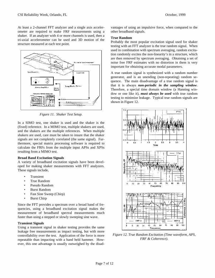
When impact testing cannot be used, FRF measurements must be made by providing artificial excitation with one or more shakers, attached to the structure. Common types of shakers are electro-dynamic and hydraulic shakers. A typical shaker test is depicted in Figure 11.

A shaker is usually attached to the structure using a stinger (long slender rod), so that the shaker will only impart force to the structure along the axis of the stinger, the axis of force measurement. A load cell is then attached between the struc-ture and the stinger to measure the excitation force.


of 12

At least a 2-channel FFT analyzer and a single axis acceler-ometer are required to make FRF measurements using a shaker. If an analyzer with 4 or more channels is used, then a tri-axial accelerometer can be used and 3D motion of the structure measured at each test point.

Figure 11. Shaker Test Setup.

In a SIMO test, one shaker is used and the shaker is the (fixed) reference. In a MIMO test, multiple shakers are used, and the shakers are the multiple references. When multiple shakers are used, care must be taken to insure that the shaker signals are not completely correlated (the same signal). Fur-thermore, special matrix processing software is required to calculate the FRFs from the multiple input APSs and XPSs resulting from a MIMO test.

Broad Band Excitation Signals A variety of broadband excitation signals have been devel-oped for making shaker measurements with FFT analyzers. These signals include,

• Transient • True Random • Pseudo Random • Burst Random • Fast Sine Sweep (Chirp) • Burst Chirp

Since the FFT provides a spectrum over a broad band of fre-quencies, using a broadband excitation signal makes the measurement of broadband spectral measurements much faster than using a stepped or slowly sweeping sine wave.

Transient Signals Using a transient signal in shaker testing provides the same leakage free measurements as impact testing, but with more controllability over the test. Application of the force is more repeatable than impacting with a hand held hammer. How-ever, this one advantage is usually outweighed by the disad-

vantages of using an impulsive force, when compared to the other broadband signals.

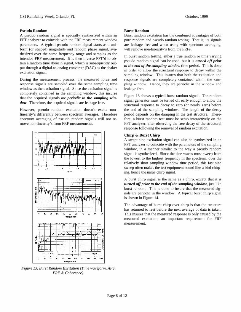
True Random Probably the most popular excitation signal used for shaker testing with an FFT analyzer is the true random signal. When used in combination with spectrum averaging, random excita-tion randomly excites the non-linearity’s in a structure, which are then removed by spectrum averaging. Obtaining a set of noise free FRF estimates with no distortion in them is very important for obtaining accurate modal parameters.

A true random signal is synthesized with a random number generator, and is an unending (non-repeating) random se-quence. The main disadvantage of a true random signal is that it is always non-periodic in the sampling window. Therefore, a special time domain window (a Hanning win-dow or one like it), must always be used with true random testing to minimize leakage. Typical true random signals are shown in Figure 12.

Figure 12. True Random Excitation (Time waveform, APS, FRF & Coherence).


of 12

Pseudo Random A pseudo random signal is specially synthesized within an FFT analyzer to coincide with the FRF measurement window parameters. A typical pseudo random signal starts as a uni-form (or shaped) magnitude and random phase signal, syn-thesized over the same frequency range and samples as the intended FRF measurement. It is then inverse FFT’d to ob-tain a random time domain signal, which is subsequently out-put through a digital-to-analog converter (DAC) as the shaker excitation signal.

During the measurement process, the measured force and response signals are sampled over the same sampling time window as the excitation signal. Since the excitation signal is completely contained in the sampling window, this insures that the acquired signals are periodic in the sampling win-dow. Therefore, the acquired signals are leakage free.

However, pseudo random excitation doesn’t excite non-linearity’s differently between spectrum averages. Therefore spectrum averaging of pseudo random signals will not re-move non-linearity’s from FRF measurements.

Figure 13. Burst Random Excitation (Time waveform, APS, FRF & Coherence).

Burst Random Burst random excitation has the combined advantages of both pure random and pseudo random testing. That is, its signals are leakage free and when using with spectrum averaging, will remove non-linearity’s from the FRFs.

In burst random testing, either a true random or time varying pseudo random signal can be used, but it is turned off prior to the end of the sampling window time period. This is done in order to allow the structural response to decay within the sampling window. This insures that both the excitation and response signals are completely contained within the sam-pling window. Hence, they are periodic in the window and leakage free.

Figure 13 shows a typical burst random signal. The random signal generator must be turned off early enough to allow the structural response to decay to zero (or nearly zero) before the end of the sampling window. The length of the decay period depends on the damping in the test structure. There-fore, a burst random test must be setup interactively on the FFT analyzer, after observing the free decay of the structural response following the removal of random excitation.

Chirp & Burst Chirp A swept sine excitation signal can also be synthesized in an FFT analyzer to coincide with the parameters of the sampling window, in a manner similar to the way a pseudo random signal is synthesized. Since the sine waves must sweep from the lowest to the highest frequency in the spectrum, over the relatively short sampling window time period, this fast sine sweep often makes the test equipment sound like a bird chirp-ing, hence the name chirp signal.

A burst chirp signal is the same as a chirp, except that it is turned off prior to the end of the sampling window, just like burst random. This is done to insure that the measured sig-nals are periodic in the window. A typical burst chirp signal is shown in Figure 14.

The advantage of burst chirp over chirp is that the structure has returned to rest before the next average of data is taken. This insures that the measured response is only caused by the measured excitation, an important requirement for FRF measurement.


of 12

Figure 14. Burst Chirp Excitation (Time waveform, APS, FRF & Coherence)

Comparison of Excitation Signals Ideally, all of the shaker signals that are leakage free (peri-odic in the window) should yield the same results. Figure 15 shows an overlay of two FRF magnitudes, one measured with a burst random test and the other with a burst chirp test. The two FRFs match very well at low frequencies, but show some disparity at high frequencies. This could possibly be due to a small amount of non-linear behavior in the structure, which burst chirp signal processing cannot remove through averaging.

HOW ARE MODAL PARAMETERS OBTAINED?

Figure 16 shows the different ways in which modal parame-ters can be obtained, both analytically and experimentally. A growing amount of finite element modeling, with extraction of modal parameters from the finite element model, is being done in an effort to understand and solve structural dynamics problems. Experimental modal analysis is also done for this same purpose.

Figure 15. Burst Random Versus Burst Chirp FRF.

The majority of modern experimental modal analysis relies upon the application of a modal parameter estimation (curve fitting) technique to a set of FRF measurements. As indi-cated in Figure 16, the FRFs can also be inverse FFT’d and curve fitting techniques applied to their equivalent Impulse Response Functions (IRFs).

Figure 16. Sources of Modal Parameters.

MODAL PARAMETERS FROM CURVE FITTING

Modal parameters are most commonly identified by curve fitting a set of FRFs. (They can also be identified by curve fitting an equivalent set of Impulse Responses, or IRFs). In general, curve fitting is a process of matching a mathematical expression to a set of empirical data points. This is done by minimizing the squared error (or squared difference) be-


of 12

tween the analytical function and the measured data. An ex-ample of FRF curve fitting is shown in Figure 17.

Figure 17. A Curve Fitting Example.

CURVE FITTING METHODS

All curve fitting methods fall into one of the following cate-gories,

• Local SDOF • Local MDOF • Global • Multi-Reference (Poly Reference)

In general, the methods are listed in order of increasing com-plexity. SDOF is short for a Single Degree Of Freedom, or single mode method. Similarly, MDOF is short for a Multi-ple Degree Of Freedom, or multiple mode method.

SDOF methods estimate modal parameters one mode at a time. MDOF, Global, and Multi-Reference methods can simultaneously estimate modal parameters for two or more modes at a time.

Local methods are applied to one FRF at a time. Global and Multi-Reference methods are applied to an entire set of FRFs at once.

Local SDOF methods are the easiest to use, and should be used whenever possible. SDOF methods can be applied to most FRF data sets with light modal density (coupling), as depicted in Figure 19. MDOF methods must be used in cases of high modal density.

Global methods work much better than MDOF methods for cases with local modes. Multi-Reference methods can find repeated roots (very closely coupled modes) where the other methods cannot.

Figure 19. Light Versus Heavy Modal Density (Coupling).

Local SDOF Methods Figure 20 depicts the three most commonly used curve-fitting methods for obtaining modal parameters. These are referred to as SDOF (single degree of freedom, or single mode) meth-ods. Even though they don’t look like curve fitting methods (in the sense of fitting a curve to empirical data), all three of these methods are based on applying an analytical expression for the FRF to measured data [3].

Modal Frequency as Peak Frequency The frequency of a resonance peak in the FRF is used as the modal frequency. This peak frequency, which is also de-pendent on the frequency resolution of the measurements, is not exactly equal to the modal frequency but is a close ap-proximation, especially for lightly damped structures. The resonance peak should appear at the same frequency in al-most every FRF measurement. It won’t appear in those measurements corresponding to nodal lines (zero magnitude) of the mode shape.

Figure 20. Curve Fitting FRF Measurements.


of 12

Modal Damping as Peak Width The width of the resonance peak is a measure of modal damping. The resonance peak width should also be the same for all FRF measurements, meaning that modal damping is the same in every FRF measurement. The width is actually measured at the so-called half power point, and is approxi-mately equal to twice the modal damping (in Hz).

Mode Shape From Quadrature Peaks From (displacement/force) or (acceleration/force) FRFs, the peak values of the imaginary part of the FRFs are taken as components of the mode shape. This is called the Quadra-ture method of curve fitting. From (velocity/force) FRFs, the peak values of the real part are used as mode shape compo-nents.

Hence, using the simplest Local SDOF curve fitting methods, all three modal parameters (frequency, damping, and mode shape) can be extracted directly from a set of FRF measure-ments.

Local MDOF Methods The Complex Exponential and the Rational Fraction Poly-nomial methods are two of the most popular Local MDOF curve fitting methods.

Complex Exponential (CE) This algorithm curve fits and analytical expression for a structural impulse response to experimental impulse response data. A set of impulse response data is normally obtained by applying the Inverse FFT to a set of FRF measurements, as shown in Figure 16.

Figure 21 shows the analytical expression used by Complex Exponential curve fitting. Also pointed out in Figure 20 is the leakage (wrap around error) caused by the inverse FFT, which distorts the impulse response data. This portion of the data cannot be used because of this error.

Figure 21. CE Curve Fitting.

Rational Fraction Polynomial (RFP) This method applies the rational fraction polynomial expres-sion shown in Figure 22 directly to an FRF measurement. Its advantage is that it can be applied over any frequency range of data, and particularly in the vicinity of a resonance peak.

Figure 22. Alternate Curve Fitting Forms of the FRF.

As shown in Figure 23, not only can the RFP method be used to estimate modal parameters, but it also yields the numera-tor & denominator polynomial coefficients, as well as the poles & zeros of the FRF.

Figure 23. RFP Solution Method.

Global and Multi-Reference Methods Both the CE and RFP algorithms have been implemented as Global and Multi-Reference methods also. The details of these methods are given in references [4] through [6].


of 12

CONCLUSIONS

Modern experimental modal analysis techniques have been reviewed in this paper. The three main topics pertaining to modal testing; FRF measurement techniques, excitation tech-niques, and modal parameter estimation (curve fitting) meth-ods were covered.

FRF based modal testing started in the early 1970’s with the commercial availability of the digital FFT analyzer, and has grown steadily in popularity since then. The modern modal testing techniques presented here are just a brief summary of the accumulation of the past 30 years of progress.

REFERENCES

[1] Potter, R. and Richardson, M.H. "Identification of the Modal Properties of an Elastic Structure from Measured Transfer Function Data" 20th International Instrumentation Symposium, Albuquerque, New Mexico, May 1974.

[2] Rocklin, G.T, Crowley, J., and Vold, H. “A Comparison of H1, H2, and HV Frequency Response Functions“, 3rd Inter-national Modal Analysis Conference, Orlando FL, January 1985.

[3] Richardson, M. H., "Modal Analysis Using Digital Test Systems," Seminar on Understanding Digital Control and Analysis in Vibration Test Systems, Shock and Vibration Information Center Publication, Naval Research Laboratory, Washington D.C. May 1975.

[4] Formenti, D. and Richardson, M. H., “Global Curve Fitting of Frequency Response Measurements using the Rational Frac-tion Polynomial Method", 3rd International Modal Analysis Conference, Orlando, FL, January 1985.

[5] Formenti, D. and Richardson, M. H. “Global Frequency & Damping from Frequency Response Measurements", 4th Inter-national Modal Analysis Conference, Los Angeles, CA, Febru-ary 1986

[6] Vold, H. and Rocklin, G.T., “The Numerical Implementa-tion of a Multi-Input Estimation Method for Mini-Computers”, 1st International Modal Analysis Conference, Orlando, FL, Sep-tember 1982.

EXPERIMENTAL MODAL ANALYSIS vibration is a combination of both forced and resonant vibration. Forced...

Documents

Transcript of EXPERIMENTAL MODAL ANALYSIS vibration is a combination of both forced and resonant vibration. Forced...