Experimental Investigation of Rotor Vortex Wakes in

Descent

James Stack∗†

University of California Berkeley, Berkeley, CA 94720-1742jstack@me.berkeley.edu

January 5, 2004

An experimental study is performed on a three-bladed rotor model in a water tow tank. Therotor’s rotational velocity, the rotor plane angle of attack, and the carriage speed are all variedin order to simulate a wide range of rotorcraft operating states. The focus is on descent speedsand angles where the rotor is operating in or near vortex ring state. Circulation Reynoldsnumbers are of order 105 and chord Reynolds numbers are of order 104. Flow visualization isdone using air bubbles and fluorescent dye injected tangentially from the blade tips to markthe vortex core, showing the development of both short-wave and long-wave instabilities onthe helical vortices in the wake. Strain gages are used to record transient loads, allowing acorrelation between the rotor thrust performance and the development of the vortex wake.The data indicate that as the instability develops, the adjacent vortices merge and formthick vortex rings, especially during descent. Periodic shedding of vorticity from the wakeassociated with vortex ring state is observed, resulting in peak-to-peak thrust fluctuationsof up to 95% of the mean and occurring at regular intervals of 20 − 50 rotor revolutions,depending on flow parameters.

Nomenclaturec = blade chord

A = rotor disk area, πR2

CT = thrust coefficient, T/ρAV 2tipR = rotor radius

Rec = Reynolds number based on chord, Vtipc/ν

T = rotor thrust

V = towing speed

Vtip = rotor tip speed, ΩR

Vx = rotor forward flight speed, V cosα

Vz = rotor descent speed, V sinα

α = descent angle

λ = short-wave instability wavelength

µ = rotor advance ratio, Vx/Vtipν = kinematic viscosity

ξ = rotor descent ratio, Vz/Vtipρ = water density

σ = standard deviation from mean rotor thrust

∗AIAA Student Member, No. 210930†Faculty advisor: Professor Omer Savas, AIAA Associate

Fellow

θ = rotor collective pitch angle

Ω = rotor rotational speed

Introduction

An accurate understanding of the physics of he-

lical vortex wakes has long been regarded as one of

the most difficult problems in fluid dynamics. With

implications on the performance of propellers, wind

turbines, and helicopter rotors, the problem is of

practical interest to many. Even before the days

of modern production helicopter flight, the issue of

the nature and stability of ring vortices and helical

vortices had been analyzed extensively. Levy and

Forsdyke1 performed a stability analysis on a sin-

gle helical vortex in 1928, and more recently, Land-

grebe2 and Widnall3 have added to and corrected

this study. Gupta and Loewy4 have performed a

similar analysis on multiple interdigitated helical

vortices. Despite the focus that modern helicopter

flight has brought to the problem in the last hundred

1

years, and despite the power of modern computers

and experimental tools, a true grasp of the physics

of helical vortices has remained elusive. While some-

what reasonable approximations of their behavior

can be made under restricted and simplified sce-

narios, there is a great deal of progress still to be

made on the problem of real helical vortices. In fact,

not even the simplest case of a stationary (hovering)

rotor generating a steady vertical helical wake can

be computationally modelled with much accuracy at

distances greater than a few diameters downstream

of the rotor.

In the early days of helicopter flight, a num-

ber of simple models appeared — such as the clas-

sic momentum theory and the blade element mo-

mentum theory5,6 — which were capable of pre-

dicting gross performance characteristics for a ro-

tor (such as thrust and power) but were unable

to capture the detailed dynamics of the wake flow-

field. Realizing the powerful effect of the wake

on the rotor performance, researchers began more

detailed studies of the wake flow field, beginning

with wind tunnel testing and smoke flow visualiza-

tion as early as the 1920s.7—9 Later, experiments

were done using hot wire anemometry (HWA) and

other probe techniques10 to measure the velocity

field itself. Even more recent work has used laser

Doppler velocimetry (LDV)11—13 and particle im-

age velocimetry (PIV)14,15 as non-invasive means of

achieving the same. The power of modern comput-

ers has recently been harnessed by researchers using

more sophisticated, detailed models of the flow field.

Current methods in computational fluid dynamics

(CFD) utilize ‘free wake analysis’, attempting to cal-

culate the velocity that is induced at a point by all of

the vortices in the wake as well as by the blades.16,17

And while CFD techniques have led to significant

progress over the past ten years in the understand-

ing of simpler cases of flight such as hover, they are

not yet capable of predicting the behavior of the

wake in more complicated flight states where the air-

craft is maneuvering or descending. They are also

inadequate for dealing with the true complexities of

rotorcraft flight like blade stall, airframe interaction,

main rotor/tail rotor interaction, shock waves, and

turbulence.18

The problem for aerodynamicists is that the flight

regimes in which CFD predictions are least accurate

are precisely the ones that are of greatest interest

to the rotorcraft community. When a helicopter is

descending rapidly, the very thing that makes the

wake solution so difficult — the intense interaction

between the rotor and its vortex wake — causes large,

unsteady dynamic loads on the blades. Under the

right circumstances (when the rotor descent veloc-

ity approximately matches the wake velocity), this

condition, known as vortex ring state (VRS), can

cause the tip vortices to merge together, forming a

thick vortex ring that remains near the rotor plane,

disrupting the inflow and causing a dramatic reduc-

tion in lift. This unstable ring typically undergoes a

chaotic shedding and re-formation pattern that re-

sults in large fluctuations in thrust that make the

aircraft quite difficult to control. As retired test pilot

Mott F. Stanchfield says, “In my opinion, a mature

VRS is the most hazardous condition that exists in

the realm of helicopter aeronautics.”19 In fact, VRS

has been identified as the likely cause of the April

8, 2000 crash of the Marine’s V-22 Osprey tiltrotor

aircraft near Marana, Arizona. In this operations

test accident, it is believed that the aircraft — oper-

ating in helicopter mode — experienced VRS on its

right rotor only, causing it to bank sharply and then

nose-dive 250 ft to the ground, killing all 19 peo-

ple on board.20 Prior to this event it was not widely

known that a dual-rotor craft would experience such

an unusual roll control problem in VRS, which illus-

trates just how poorly understood this condition still

is today.

The purpose of the present experimental study is

to explore the physics of the wake evolution in VRS

and other descent configurations. Flow visualization

and thrust measurement results are presented from

experiments performed on a model rotor in a wide

range of operating states — from hover to forward

flight to rapid descent — with the main focus being

on the vortex ring state regime. Experiments were

performed in a 70 m long water tunnel, which al-

lowed for much longer test runs than have previously

been performed in similar studies (which have gen-

erally been conducted in wind tunnels).21,22 The

rotor’s performance is quantified by measurements

of its thrust, and this information is correlated with

flow visualization images.

The time-history characteristics of the rotor’s

thrust are examined for a broad range of descent

2

speed and angle combinations. By testing the ro-

tor’s performance over a wide variety of configura-

tions, the rotor’s performance characteristics can be

fully characterized, and the descent conditions in

which VRS behavior is observed can be clearly iden-

tified. The thrust histories of these periodic shed-

ding cases are then compared in order to determine

how the descent configuration affects the amplitude,

frequency, and overall “orderliness” of the observed

fluctuations. For these particular cases, the flow vi-

sualization images of the experiment are expected to

provide clues as to the nature of the vortex wake for-

mation and shedding phenomenon that makes VRS

such a dangerous flight regime.

Experimental Setup

Rotor Model

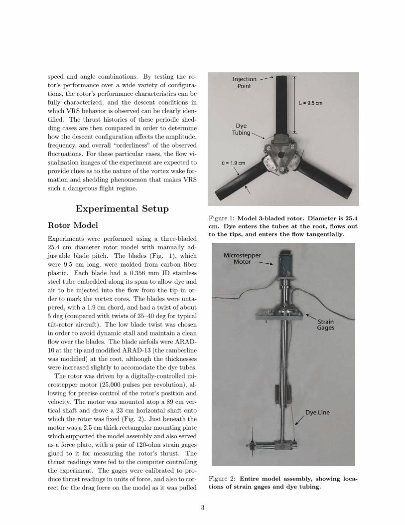
Experiments were performed using a three-bladed

25.4 cm diameter rotor model with manually ad-

justable blade pitch. The blades (Fig. 1), which

were 9.5 cm long, were molded from carbon fiber

plastic. Each blade had a 0.356 mm ID stainless

steel tube embedded along its span to allow dye and

air to be injected into the flow from the tip in or-

der to mark the vortex cores. The blades were unta-

pered, with a 1.9 cm chord, and had a twist of about

5 deg (compared with twists of 35—40 deg for typical

tilt-rotor aircraft). The low blade twist was chosen

in order to avoid dynamic stall and maintain a clean

flow over the blades. The blade airfoils were ARAD-

10 at the tip and modified ARAD-13 (the camberline

was modified) at the root, although the thicknesses

were increased slightly to accomodate the dye tubes.

The rotor was driven by a digitally-controlled mi-

crostepper motor (25,000 pulses per revolution), al-

lowing for precise control of the rotor’s position and

velocity. The motor was mounted atop a 89 cm ver-

tical shaft and drove a 23 cm horizontal shaft onto

which the rotor was fixed (Fig. 2). Just beneath the

motor was a 2.5 cm thick rectangular mounting plate

which supported the model assembly and also served

as a force plate, with a pair of 120-ohm strain gages

glued to it for measuring the rotor’s thrust. The

thrust readings were fed to the computer controlling

the experiment. The gages were calibrated to pro-

duce thrust readings in units of force, and also to cor-

rect for the drag force on the model as it was pulled

Figure 1: Model 3-bladed rotor. Diameter is 25.4cm. Dye enters the tubes at the root, flows out

to the tips, and enters the flow tangentially.

Figure 2: Entire model assembly, showing loca-tions of strain gages and dye tubing.

3

through the water. A bandpass filter was used to

eliminate high-frequency electrical and vibrational

noise while retaining the important details.

To visualize the rotor’s wake, air bubbles and

sodium fluorescent dye were leaked from the blade

tips in a direction tangential to the blade path. The

dye and air were supplied to the dye reservoir at the

base of the vertical shaft through thin plastic tubing

(Fig. 2). The dye reservoir was directly connected

to the rotor dye tubes through the horizontal drive

shaft. The pressure deficit in the vortex cores drew

some fluid into the wake, but in order to achieve

clear visualization of the flow it was necessary to

force additional dye or air to the blades using an

external pressurized canister.

Stationary Tank

Initial testing was performed in a 1.22 × 2.44 × 1.68m deep stationary water tank. With the model fixed

in place on top of the tank, this test simulated a

hovering helicopter’s flow field. A 10-W Argon ion

laser was used for both two- and three-dimensional

illumination. For the two-dimensional lighting tests,

a vertical light sheet was aligned with the axis of the

rotor. In all cases, a digital video camera recorded

the flow from the side of the tank, perpendicular to

the wake direction and the light sheet.

Generally, air was used as the injection fluid for

initial experiments because of its non-contaminating

nature. The buoyancy of the bubbles, however,

caused them to rise to the surface quickly, render-

ing the details of the wake incoherent for distances

greater than about one diameter downstream of the

rotor. In the near-wake of the rotor, however, the air

bubbles could better capture the details of the vortex

filaments. Later tests used neutrally-buoyant fluo-

rescent dye as the injection fluid, which more clearly

showed the break-up and diffusion of the wake at

greater downstream distances. No thrust measure-

ments were recorded for any of the stationary tank

tests. Rather, these tests were performed solely for

visualization purposes, as the quality of the images

was significantly better in the stationary tank than

in the towing tank.

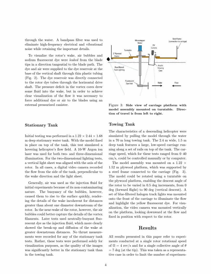
Figure 3: Side view of carriage platform with

model assembly mounted on turntable. Direc-

tion of travel is from left to right.

Towing Tank

The characteristics of a descending helicopter were

simulated by pulling the model through the water

in a 70 m long towing tank. The 2.4 m wide, 1.5 m

deep tank features a large, low-speed carriage run-

ning along a set of rails on top of the tank. The car-

riage speed, which for these tests ranged from 0—40

cm/s, could be controlled manually or by computer.

The model assembly was mounted on a 1.22 ×1.52 m plywood platform, which was supported by

a steel frame connected to the carriage (Fig. 3).

The model could be rotated using a turntable on

the plywood platform, enabling the descent angle of

the rotor to be varied in 0.5 deg increments, from 0

deg (forward flight) to 90 deg (vertical descent). A

set of blue-filtered halogen track lights was mounted

onto the front of the carriage to illuminate the flow

and highlight the yellow fluorescent dye. For visu-

alization, the video camera was mounted vertically

on the platform, looking downward at the flow and

fixed in position with respect to the rotor.

Results

All results presented in this paper refer to experi-

ments conducted at a single rotor rotational speed

of Ω = 4 rev/s and for a single collective angle of θ

= 7 deg (at the tip). This was taken as a representa-

tive case in order to limit the number of experimen-

4

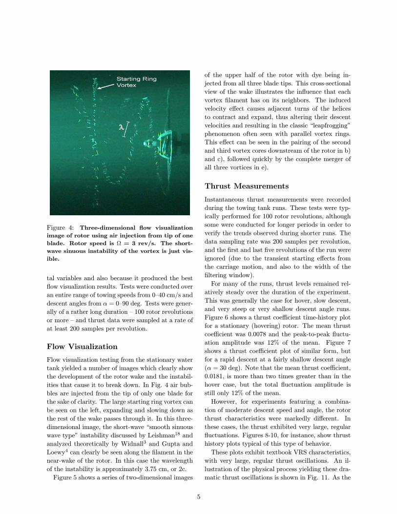
Figure 4: Three-dimensional flow visualization

image of rotor using air injection from tip of one

blade. Rotor speed is Ω = 3 rev/s. The short-

wave sinuous instability of the vortex is just vis-

ible.

tal variables and also because it produced the best

flow visualization results. Tests were conducted over

an entire range of towing speeds from 0—40 cm/s and

descent angles from α = 0—90 deg. Tests were gener-

ally of a rather long duration — 100 rotor revolutions

or more — and thrust data were sampled at a rate of

at least 200 samples per revolution.

Flow Visualization

Flow visualization testing from the stationary water

tank yielded a number of images which clearly show

the development of the rotor wake and the instabil-

ities that cause it to break down. In Fig. 4 air bub-

bles are injected from the tip of only one blade for

the sake of clarity. The large starting ring vortex can

be seen on the left, expanding and slowing down as

the rest of the wake passes through it. In this three-

dimensional image, the short-wave “smooth sinuous

wave type” instability discussed by Leishman18 and

analyzed theoretically by Widnall3 and Gupta and

Loewy4 can clearly be seen along the filament in the

near-wake of the rotor. In this case the wavelength

of the instability is approximately 3.75 cm, or 2c.

Figure 5 shows a series of two-dimensional images

of the upper half of the rotor with dye being in-

jected from all three blade tips. This cross-sectional

view of the wake illustrates the influence that each

vortex filament has on its neighbors. The induced

velocity effect causes adjacent turns of the helices

to contract and expand, thus altering their descent

velocities and resulting in the classic “leapfrogging”

phenomenon often seen with parallel vortex rings.

This effect can be seen in the pairing of the second

and third vortex cores downstream of the rotor in b)

and c), followed quickly by the complete merger of

all three vortices in e).

Thrust Measurements

Instantaneous thrust measurements were recorded

during the towing tank runs. These tests were typ-

ically performed for 100 rotor revolutions, although

some were conducted for longer periods in order to

verify the trends observed during shorter runs. The

data sampling rate was 200 samples per revolution,

and the first and last five revolutions of the run were

ignored (due to the transient starting effects from

the carriage motion, and also to the width of the

filtering window).

For many of the runs, thrust levels remained rel-

atively steady over the duration of the experiment.

This was generally the case for hover, slow descent,

and very steep or very shallow descent angle runs.

Figure 6 shows a thrust coefficient time-history plot

for a stationary (hovering) rotor. The mean thrust

coefficient was 0.0078 and the peak-to-peak fluctu-

ation amplitude was 12% of the mean. Figure 7

shows a thrust coefficient plot of similar form, but

for a rapid descent at a fairly shallow descent angle

(α = 30 deg). Note that the mean thrust coefficient,

0.0181, is more than two times greater than in the

hover case, but the total fluctuation amplitude is

still only 12% of the mean.

However, for experiments featuring a combina-

tion of moderate descent speed and angle, the rotor

thrust characteristics were markedly different. In

these cases, the thrust exhibited very large, regular

fluctuations. Figures 8-10, for instance, show thrust

history plots typical of this type of behavior.

These plots exhibit textbook VRS characteristics,

with very large, regular thrust oscillations. An il-

lustration of the physical process yielding these dra-

matic thrust oscillations is shown in Fig. 11. As the

5

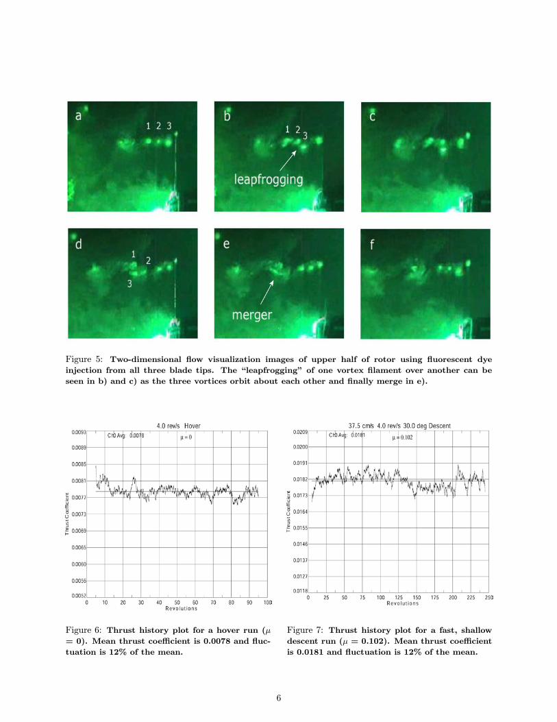
Figure 5: Two-dimensional flow visualization images of upper half of rotor using fluorescent dye

injection from all three blade tips. The “leapfrogging” of one vortex filament over another can be

seen in b) and c) as the three vortices orbit about each other and finally merge in e).

Figure 6: Thrust history plot for a hover run (µ= 0). Mean thrust coefficient is 0.0078 and fluc-

tuation is 12% of the mean.

Figure 7: Thrust history plot for a fast, shallowdescent run (µ = 0.102). Mean thrust coefficient

is 0.0181 and fluctuation is 12% of the mean.

6

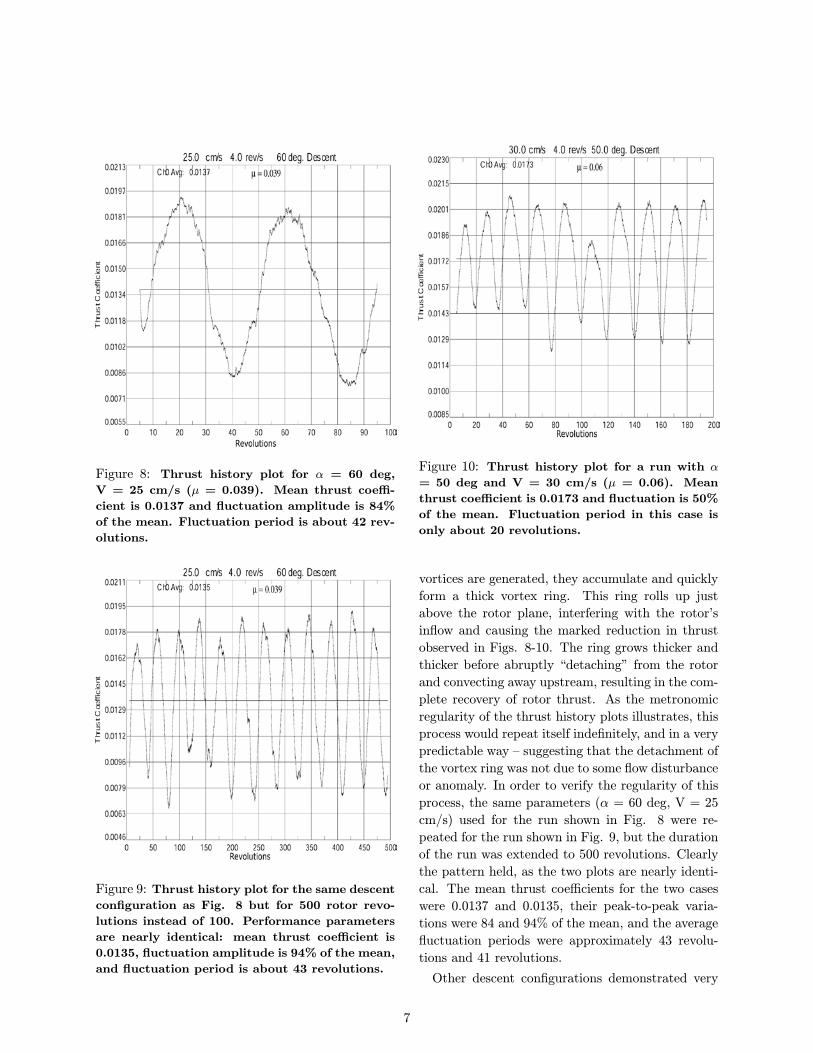
Figure 8: Thrust history plot for α = 60 deg,

V = 25 cm/s (µ = 0.039). Mean thrust coeffi-

cient is 0.0137 and fluctuation amplitude is 84%

of the mean. Fluctuation period is about 42 rev-

olutions.

Figure 9: Thrust history plot for the same descentconfiguration as Fig. 8 but for 500 rotor revo-

lutions instead of 100. Performance parameters

are nearly identical: mean thrust coefficient is

0.0135, fluctuation amplitude is 94% of the mean,

and fluctuation period is about 43 revolutions.

Figure 10: Thrust history plot for a run with α

= 50 deg and V = 30 cm/s (µ = 0.06). Mean

thrust coefficient is 0.0173 and fluctuation is 50%

of the mean. Fluctuation period in this case is

only about 20 revolutions.

vortices are generated, they accumulate and quickly

form a thick vortex ring. This ring rolls up just

above the rotor plane, interfering with the rotor’s

inflow and causing the marked reduction in thrust

observed in Figs. 8-10. The ring grows thicker and

thicker before abruptly “detaching” from the rotor

and convecting away upstream, resulting in the com-

plete recovery of rotor thrust. As the metronomic

regularity of the thrust history plots illustrates, this

process would repeat itself indefinitely, and in a very

predictable way — suggesting that the detachment of

the vortex ring was not due to some flow disturbance

or anomaly. In order to verify the regularity of this

process, the same parameters (α = 60 deg, V = 25

cm/s) used for the run shown in Fig. 8 were re-

peated for the run shown in Fig. 9, but the duration

of the run was extended to 500 revolutions. Clearly

the pattern held, as the two plots are nearly identi-

cal. The mean thrust coefficients for the two cases

were 0.0137 and 0.0135, their peak-to-peak varia-

tions were 84 and 94% of the mean, and the average

fluctuation periods were approximately 43 revolu-

tions and 41 revolutions.

Other descent configurations demonstrated very

7

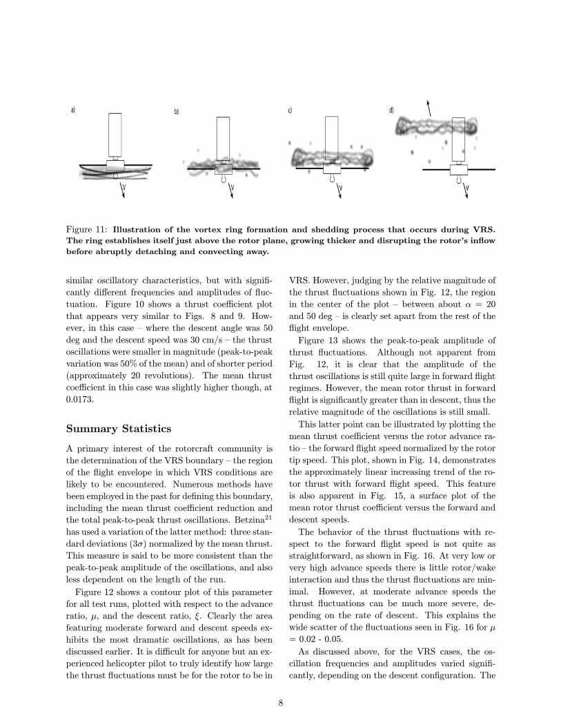
Figure 11: Illustration of the vortex ring formation and shedding process that occurs during VRS.

The ring establishes itself just above the rotor plane, growing thicker and disrupting the rotor’s inflow

before abruptly detaching and convecting away.

similar oscillatory characteristics, but with signifi-

cantly different frequencies and amplitudes of fluc-

tuation. Figure 10 shows a thrust coefficient plot

that appears very similar to Figs. 8 and 9. How-

ever, in this case — where the descent angle was 50

deg and the descent speed was 30 cm/s — the thrust

oscillations were smaller in magnitude (peak-to-peak

variation was 50% of the mean) and of shorter period

(approximately 20 revolutions). The mean thrust

coefficient in this case was slightly higher though, at

0.0173.

Summary Statistics

A primary interest of the rotorcraft community is

the determination of the VRS boundary — the region

of the flight envelope in which VRS conditions are

likely to be encountered. Numerous methods have

been employed in the past for defining this boundary,

including the mean thrust coefficient reduction and

the total peak-to-peak thrust oscillations. Betzina21

has used a variation of the latter method: three stan-

dard deviations (3σ) normalized by the mean thrust.

This measure is said to be more consistent than the

peak-to-peak amplitude of the oscillations, and also

less dependent on the length of the run.

Figure 12 shows a contour plot of this parameter

for all test runs, plotted with respect to the advance

ratio, µ, and the descent ratio, ξ. Clearly the area

featuring moderate forward and descent speeds ex-

hibits the most dramatic oscillations, as has been

discussed earlier. It is difficult for anyone but an ex-

perienced helicopter pilot to truly identify how large

the thrust fluctuations must be for the rotor to be in

VRS. However, judging by the relative magnitude of

the thrust fluctuations shown in Fig. 12, the region

in the center of the plot — between about α = 20

and 50 deg — is clearly set apart from the rest of the

flight envelope.

Figure 13 shows the peak-to-peak amplitude of

thrust fluctuations. Although not apparent from

Fig. 12, it is clear that the amplitude of the

thrust oscillations is still quite large in forward flight

regimes. However, the mean rotor thrust in forward

flight is significantly greater than in descent, thus the

relative magnitude of the oscillations is still small.

This latter point can be illustrated by plotting the

mean thrust coefficient versus the rotor advance ra-

tio — the forward flight speed normalized by the rotor

tip speed. This plot, shown in Fig. 14, demonstrates

the approximately linear increasing trend of the ro-

tor thrust with forward flight speed. This feature

is also apparent in Fig. 15, a surface plot of the

mean rotor thrust coefficient versus the forward and

descent speeds.

The behavior of the thrust fluctuations with re-

spect to the forward flight speed is not quite as

straightforward, as shown in Fig. 16. At very low or

very high advance speeds there is little rotor/wake

interaction and thus the thrust fluctuations are min-

imal. However, at moderate advance speeds the

thrust fluctuations can be much more severe, de-

pending on the rate of descent. This explains the

wide scatter of the fluctuations seen in Fig. 16 for µ

= 0.02 - 0.05.

As discussed above, for the VRS cases, the os-

cillation frequencies and amplitudes varied signifi-

cantly, depending on the descent configuration. The

8

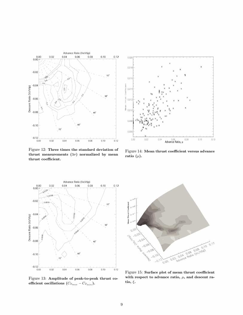
Figure 12: Three times the standard deviation ofthrust measurements (3σ) normalized by mean

thrust coefficient.

Figure 13: Amplitude of peak-to-peak thrust co-efficient oscillations (CTmax − CTmin).

Figure 14: Mean thrust coefficient versus advanceratio (µ).

Figure 15: Surface plot of mean thrust coefficientwith respect to advance ratio, µ, and descent ra-

tio, ξ.

9

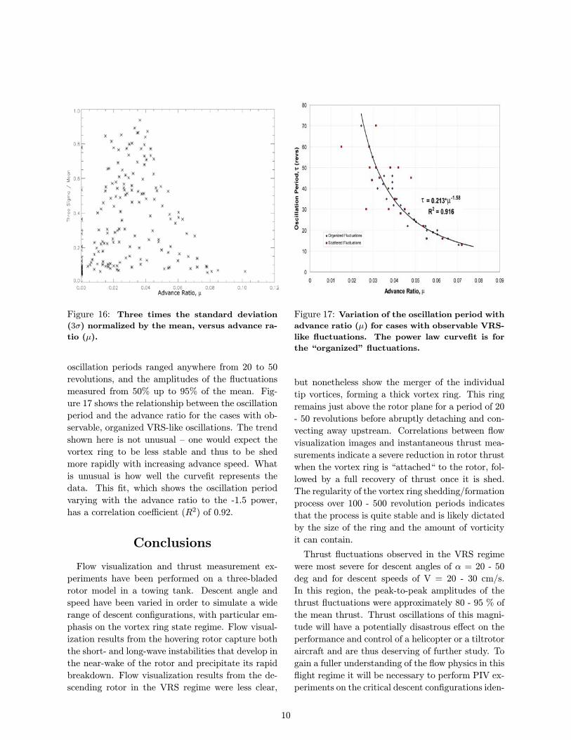
Figure 16: Three times the standard deviation

(3σ) normalized by the mean, versus advance ra-

tio (µ).

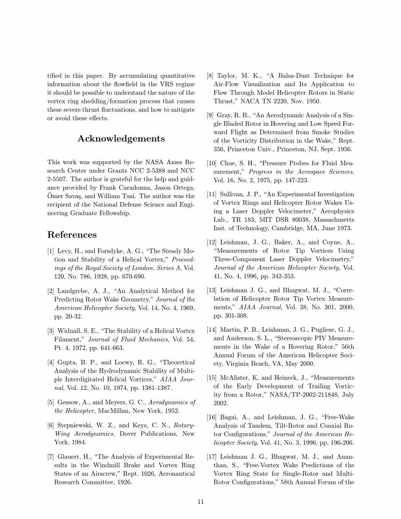
oscillation periods ranged anywhere from 20 to 50

revolutions, and the amplitudes of the fluctuations

measured from 50% up to 95% of the mean. Fig-

ure 17 shows the relationship between the oscillation

period and the advance ratio for the cases with ob-

servable, organized VRS-like oscillations. The trend

shown here is not unusual — one would expect the

vortex ring to be less stable and thus to be shed

more rapidly with increasing advance speed. What

is unusual is how well the curvefit represents the

data. This fit, which shows the oscillation period

varying with the advance ratio to the -1.5 power,

has a correlation coefficient (R2) of 0.92.

Conclusions

Flow visualization and thrust measurement ex-

periments have been performed on a three-bladed

rotor model in a towing tank. Descent angle and

speed have been varied in order to simulate a wide

range of descent configurations, with particular em-

phasis on the vortex ring state regime. Flow visual-

ization results from the hovering rotor capture both

the short- and long-wave instabilities that develop in

the near-wake of the rotor and precipitate its rapid

breakdown. Flow visualization results from the de-

scending rotor in the VRS regime were less clear,

Figure 17: Variation of the oscillation period withadvance ratio (µ) for cases with observable VRS-

like fluctuations. The power law curvefit is for

the “organized” fluctuations.

but nonetheless show the merger of the individual

tip vortices, forming a thick vortex ring. This ring

remains just above the rotor plane for a period of 20

- 50 revolutions before abruptly detaching and con-

vecting away upstream. Correlations between flow

visualization images and instantaneous thrust mea-

surements indicate a severe reduction in rotor thrust

when the vortex ring is “attached“ to the rotor, fol-

lowed by a full recovery of thrust once it is shed.

The regularity of the vortex ring shedding/formation

process over 100 - 500 revolution periods indicates

that the process is quite stable and is likely dictated

by the size of the ring and the amount of vorticity

it can contain.

Thrust fluctuations observed in the VRS regime

were most severe for descent angles of α = 20 - 50

deg and for descent speeds of V = 20 - 30 cm/s.

In this region, the peak-to-peak amplitudes of the

thrust fluctuations were approximately 80 - 95 % of

the mean thrust. Thrust oscillations of this magni-

tude will have a potentially disastrous effect on the

performance and control of a helicopter or a tiltrotor

aircraft and are thus deserving of further study. To

gain a fuller understanding of the flow physics in this

flight regime it will be necessary to perform PIV ex-

periments on the critical descent configurations iden-

10

tified in this paper. By accumulating quantitative

information about the flowfield in the VRS regime

it should be possible to understand the nature of the

vortex ring shedding/formation process that causes

these severe thrust fluctuations, and how to mitigate

or avoid these effects.

Acknowledgements

This work was supported by the NASA Ames Re-

search Center under Grants NCC 2-5388 and NCC

2-5507. The author is grateful for the help and guid-

ance provided by Frank Caradonna, Jason Ortega,

Omer Savas, and William Tsai. The author was the

recipient of the National Defense Science and Engi-

neering Graduate Fellowship.

References

[1] Levy, H., and Forsdyke, A. G., “The Steady Mo-

tion and Stability of a Helical Vortex,” Proceed-

ings of the Royal Society of London. Series A, Vol.

120, No. 786, 1928, pp. 670-690.

[2] Landgrebe, A. J., “An Analytical Method for

Predicting Rotor Wake Geometry,” Journal of the

American Helicopter Society, Vol. 14, No. 4, 1969,

pp. 20-32.

[3] Widnall, S. E., “The Stability of a Helical Vortex

Filament,” Journal of Fluid Mechanics, Vol. 54,

Pt. 4, 1972, pp. 641-663.

[4] Gupta, B. P., and Loewy, R. G., “Theoretical

Analysis of the Hydrodynamic Stability of Multi-

ple Interdigitated Helical Vortices,” AIAA Jour-

nal, Vol. 12, No. 10, 1974, pp. 1381-1387.

[5] Gessow, A., and Meyers, G. C., Aerodynamics of

the Helicopter, MacMillan, New York, 1952.

[6] Stepniewski, W. Z., and Keys, C. N., Rotary-

Wing Aerodynamics, Dover Publications, New

York, 1984.

[7] Glauert, H., “The Analysis of Experimental Re-

sults in the Windmill Brake and Vortex Ring

States of an Airscrew,” Rept. 1026, Aeronautical

Research Committee, 1926.

[8] Taylor, M. K., “A Balsa-Dust Technique for

Air-Flow Visualization and Its Application to

Flow Through Model Helicopter Rotors in Static

Thrust,” NACA TN 2220, Nov. 1950.

[9] Gray, R. B., “An Aerodynamic Analysis of a Sin-

gle Bladed Rotor in Hovering and Low Speed For-

ward Flight as Determined from Smoke Studies

of the Vorticity Distribution in the Wake,” Rept.

356, Princeton Univ., Princeton, NJ, Sept. 1956.

[10] Chue, S. H., “Pressure Probes for Fluid Mea-

surement,” Progress in the Aerospace Sciences,

Vol. 16, No. 2, 1975, pp. 147-223.

[11] Sullivan, J. P., “An Experimental Investigation

of Vortex Rings and Helicopter Rotor Wakes Us-

ing a Laser Doppler Velocimeter,” Aerophysics

Lab., TR 183, MIT DSR 80038, Massachusetts

Inst. of Technology, Cambridge, MA, June 1973.

[12] Leishman, J. G., Baker, A., and Coyne, A.,

“Measurements of Rotor Tip Vortices Using

Three-Component Laser Doppler Velocimetry,”

Journal of the American Helicopter Society, Vol.

41, No. 4, 1996, pp. 342-353.

[13] Leishman J. G., and Bhagwat, M. J., “Corre-

lation of Helicopter Rotor Tip Vortex Measure-

ments,” AIAA Journal, Vol. 38, No. 301, 2000,

pp. 301-308.

[14] Martin, P. B., Leishman, J. G., Pugliese, G. J.,

and Anderson, S. L., “Stereoscopic PIV Measure-

ments in the Wake of a Hovering Rotor,” 56th

Annual Forum of the American Helicopter Soci-

ety, Virginia Beach, VA, May 2000.

[15] McAlister, K, and Heineck, J., “Measurements

of the Early Development of Trailing Vortic-

ity from a Rotor,” NASA/TP-2002-211848, July

2002.

[16] Bagai, A., and Leishman, J. G., “Free-Wake

Analysis of Tandem, Tilt-Rotor and Coaxial Ro-

tor Configurations,” Journal of the American He-

licopter Society, Vol. 41, No. 3, 1996, pp. 196-206.

[17] Leishman J. G., Bhagwat, M. J., and Anan-

than, S., “Free-Vortex Wake Predictions of the

Vortex Ring State for Single-Rotor and Multi-

Rotor Configurations,” 58th Annual Forum of the

11

American Helicopter Society, Montreal, Canada,

June 2002.

[18] Leishman J. G., “Challenges in Understanding

the Vortex Dynamics of Helicopter Rotor Wakes,”

AIAA Journal, Vol. 36, No. 7, 1998, pp. 1130-

1140.

[19] Stanchfield, M., “Flight Dynamics: Vortex

Ring State Revisited,” Aviation Today, Nov. 2001.

[20] Ricks, T. E., “Marine Plane Crash Linked to

Unexpected Turbulence,” The Washington Post,

May 8, 2000, p. A2.

[21] Betzina, M., “Tiltrotor Descent Aerodynamics:

Small-Scale Experimental Investigation of Vortex

Ring State,” 57th Annual Forum of the American

Helicopter Society, Washington, DC, May 2001.

[22] Caradonna, F. X., “Performance Measurement

and Wake Characteristics of a Model Rotor in Ax-

ial Flight,” Journal of the American Helicopter

Society, Vol. 41, No. 4, 1996, pp. 101-108.

12