Nonlinear Dyn (2017) 90:2917–2928DOI 10.1007/s11071-017-3852-z

ORIGINAL PAPER

Experimental investigation of perpetual pointsin mechanical systems

P. Brzeski · L. N. Virgin

Received: 30 June 2017 / Accepted: 5 October 2017 / Published online: 24 October 2017© The Author(s) 2017. This article is an open access publication

Abstract In dissipative dynamical systems, equilib-rium (stationary) points have a dominant organizingeffect on transient motion in phase space, especially innonlinear systems. These time-independent solutionsare readily defined in the context of ordinary differ-ential equations, that is, they occur when all the timederivatives are simultaneously zero.However, there hasbeen some recent interest in perpetual points: points atwhich the higher time derivatives are zero, but not nec-essarily the first. Previous work has focused on analyticwork (including simulation) and some experimentalstudies of electric circuits. This paper focuses attentionon the occurrence of these points in a simple mechan-ical system, including experimental verification. Thus,points of zero acceleration can be found in which thecorresponding velocity is a maximum or minimum, butnot zero. Specifically, the rigid-arm pendulum is usedto generate data for which acceleration (and its deriva-tive) can be evaluated. In this paper an experimental(mechanical) setup is described, specifically designed

Electronic supplementary material The online version ofthis article (doi:10.1007/s11071-017-3852-z) containssupplementary material, which is available to authorized users.

P. Brzeski (B)Division of Dynamics, Lodz University of Technology,Stefanowskiego 1/15, 90-924 Lodz, Polande-mail: piotr.brzeski@p.lodz.pl

L. N. VirginDepartment of Mechanical Engineering and MaterialsScience, Duke University, Durham, NC 27708-3000, USAe-mail: l.virgin@duke.edu

to investigate perpetual points, including a descriptionof the data analysis approaches developed to identifytheir location.

Keywords Perpetual points · Mechanical systems ·Experimental investigation · Pendulum

1 Introduction

Perpetual point (PP) is a new type of critical point indynamical systems proposed in 2015 by Prasad [1]. Itis defined as a point for which all accelerations of thesystem become zero, while at least one of the veloci-ties remains nonzero. Although the role of such pointsis still not fully understood, many interesting featuresof PPs were revealed [1–3]. Thus, PPs may become auseful tool for analysis of nonlinear systems and helpto better understand some complex dynamical phenom-ena.

An intriguing topic is the possible connectionbetween PPs and hidden or rare attractors. An attractoris called rare if it has relatively small basin of attrac-tion volume,while the basin of the hidden attractor doesnot intersect with the neighborhood of any fixed point[4]. Recently, many new examples of hidden attrac-tors have been discovered [5–9] and this topic is gain-ing increasing interest. One of the challenging prob-lems is to detect and localize rare and hidden attractorsin multi-stable systems. Some sample-based methodswere proposed [10,11], but they do not reveal any infor-

123

2918 P. Brzeski, L. N. Virgin

mation on the topology of the phase space nor indicatethe mechanisms of creation of hidden or rare attrac-tors. The lack of unstable fixed points in the neighbor-hood of hidden attractors led to the hypothesis that PPscould serve as a tool to locate hidden attractors [3,4].This concept has beenwidely investigated recently, anddespite some limitations [12], PPs prove to be a usefultool to localize hidden and rare attractors in multipletypes of systems [3,13–15]. Especially in electrical sys-tems there is a need to search for efficient tool to local-ize non-trivial solutions. In [16,17] the authors presentexperimental studies of multi-stable electrical circuitswith hidden attractors and consider PPs as a possibletool to localize them in the phase space.

Initially, Prasad [1] suggested that PPs exists only indissipative systems (in the sense of Levinson [18]), butthis hypothesis is not universal as proved by Jafari et al.[19]. Apart from the above, there are papers showingthat PPs can help to better understand complex tran-sient dynamics [1], categorize chaotic flows [20] andcharacterize the attractor ruin phenomenon [21]. It islikely that more possible applications will be shortlydiscovered, especially given the current interest in PPs.

However,most of the authors refer to simple archety-pal non-dimensional models to present some generalfeatures of PPs or depict their possible applications.This is mainly because PPs are a new concept, but alsobecause in more complex dynamical models PPs maybe extremely difficult to derive analytically as largesets of nonlinear equations needs to be solved for thatpurpose. Also, there is a lack of experimental inves-tigations on the existence and characteristic of PPs inreal-world systems and, up to this point, no one hasconsidered the possibility of reaching PPs in mechan-ical systems, despite the theoretical examples basedon the types of system often used in mechanical mod-eling (e.g., Duffing’s equation and the simple pendu-lum). In this paper we investigate PPs in the context ofexperimental mechanical systems to assess their fea-sibility. We develop a simple experimental rig specif-ically designed to access PPs using only experimentaldata. Based on the obtained results we assess the appli-cability of this new mathematical concept in the fieldof experimental mechanics.

The paper is organized as follows. In Sect. 2 weinvestigate the possibility of reaching PPs in simplemechanical systems. Section 3 includes the descrip-tion of the model and parameter identification. Then,we validate the model and examine the accuracy of

numerical simulations. In Sect. 4 we present analytical,numerical and experimental investigations to localizePPs. Finally, in Sect. 5 the conclusions are given.

2 Perpetual points in mechanical systems

Mechanical systems have some specific features thatare significantwhen consideringPPs.Oneof them is thefact that they are always described by a set of second-order ordinary differential equations (ODEs)—one foreach degree of freedom (DoF) of a given system: theconfiguration space. Hence, after the transformation tothe set of first-order ODEs we get two equations pereach DoF: the phase space. Let us assume that we havethe system with n DoF each described by the general-ized coordinate xi where i = 1, 2, . . . , n. Such systemis described by the set of second-order ODEs:{xi = fi (x1, x1, x2, x2, . . . , xn, xn) , i = 1, 2, . . . , n.

(1)

After the transformation to the set of first-order ODEs,we get:{xi = vi

vi = fi (x1, v1, x2, v2, . . . , xn, vn), i = 1, 2, . . . , n.

(2)

Therefore, the state of the system is given by 2n coordi-nates xi , vi (i = 1, 2, . . . , n). Physically, xi defines thedisplacement and vi the velocity related to i th degreeof freedom. Hence, the definition of PPs for n DoFmechanical system is the following:

∀i ∈ 〈1, 2, . . . , n〉 :{xi = 0

vi = 0∧ ∃i ∈〈1, 2, . . . , n〉 : xi �= 0 ∨ vi �=0,

(3)

which, including xi = vi , can be rewritten as:

∀i ∈ 〈1, 2, . . . , n〉 :{xi = 0...x i = 0

∧ ∃i ∈ 〈1, 2, . . . , n〉 : xi �= 0. (4)

In mechanical systems xi is the acceleration and...x i

is sometimes referred to as jerk, both related to the i thdegree of freedom. This means that at the PP all accel-erations and jerks have to be equal to zero, while at leastone of the velocities should be different than zero (if

123

Experimental investigation of perpetual points in mechanical systems 2919

the velocity were zero, we would have an equilibriumpoint). The question is, whether such points exist inmechanical systems and, ultimately, whether they canbe observed experimentally.

We start our analysis with a simple, single DoF sys-tem without external excitation. This is primarily forthe sake of simplicity and because the derivation of PPsbecomesmuchmore difficult (or even impossible) withthe growth of system dimension: the curse of dimen-sionality familiarly encountered in nonlinear dynamics.We consider the physical (rigid-arm) pendulum whichis the most common paradigmatic example in nonlin-ear dynamics. PPs typically exist only in dissipativesystems, so in our example we assume the most simpleviscous damping model of dissipation. The equation ofmotion for the physical pendulum with viscous damp-ing is the following second-order ODE:

I ϕ + mgl sin (ϕ) + bϕ = 0, (5)

where I stands for the pendulum moment of inertia, mis the mass of the pendulum, l is the distance from thependulum pin joint to its center of gravity, and b is theviscous damping coefficient. After simple calculationswe reach the exact formula for PPs given as:{

ϕ = ±(n + 0.5)π

ϕ = ±mgl/bn = 1, 2, . . . (6)

We see that regardless of parameters values the PPsalways occur at ϕ = ±(n + 1/2)π . Still, the param-eters values affect the angular velocity at PPs, and inturn, the velocity at PPs determines their feasibility.To assess whether PPs can be reached experimentallywe pick some representative pendula of different scalesform different experimental investigations [11,22–27].We obtain the sets of parameter values that describe thependula from the recalled experimental rigs and calcu-

late the corresponding angular velocities at PPs. Forsome cases, we have to recalculate parameter values sothat they refer to Eq. 5. Results are presented in Table 1.

The examples shown in Table 1 reflect differentsizes and shapes of pendula. For the pendulum withsmall mass, moment of inertia and damping coefficient(# 1,3) we see that the angular velocities at PPs areextremely high (> 17, 500 rpm) and, of course, cannotbe reached in an experiment. By increasing the viscousdamping coefficient (# 2) we are able to decrease theangular velocity at PP to 2762 rpm, but it also would beinfeasible to achieve in the considered case [22]. Whenwe increase the mass, moment of inertia and damp-ing coefficient (# 5,7) we reduce the velocity at PPsto around 3000 rpm. Still, at the recalled experimen-tal rigs, such speeds would cause extreme centrifugalforces that could destroy them. By tuning the parame-ter values we are able to decrease the angular velocitiesat PPs to 647 rpm (# 4) which still is too much for theconsidered experimental setup [24]. To sum up, ana-lyzing the data presented in Table 1 we claim that forthe considered experimental realizations of a physicalpendulum it is not possible to reach PPs experimentallydue to the large angular velocities.

The above analysis proves that even for the simpleparadigmatic example of a nonlinear mechanical sys-tem we may not be able to get to PPs in an experiment.We do not consider more complex systems, but theproblem is that with the growth of complexity the for-mulas describing PPs become much more difficult toobtain. Therefore, one can conclude that for the mostof commonly analyzed mechanical systems it is barelypossible to reach PPs. Nevertheless, in this paper weshow that it is possible to design a simple experimentalsetup to facilitate the observation of PPs and analyzethem experimentally.

Table 1 Exemplar sets ofphysical pendulumparameters taken fromscientific papers andcorresponding angularvelocities at PPs

# I (kgm2) m (kg) l (m) b (Nm s) Angular velocity at PP References

rad/s rpm

1 4.47 × 10−5 0.02077 0.063 7 × 10−6 1834 17,511 [11]

2 1.74 × 10−4 0.0147 0.0475 2.37 × 10−5 289.3 2762 [22]

3 0.0084 0.22 0.1694 1.92 × 10−4 1904 18,183 [23]

4 0.0175 0.588 0.1457 0.0124 67.76 647 [24]

5 0.0216 0.42 0.194 0.0021 380.6 3635 [25]

6 0.164 0.53 0.586 0.019 160.1 1529 [26]

7 0.654 5.07 0.157 0.029 267.5 2555 [27]

123

2920 P. Brzeski, L. N. Virgin

3 Model of the system

In the paper we experimentally investigate the dynam-ics of a tilted physical pendulumwith the specific shapeas presented in Fig. 1a. Taking into account the con-clusions from the previous section we design our sys-tem to make PPs feasible. For that purpose, we add aplastic strip that increases the drag and tilt the axis ofrotation. Pendulum is mounted directly to a very lowfriction rotary motion sensor (PASCO CI-6538) whichenables precise measurement of the pendulum positionand serves as a pin joint.

In Fig. 1b we show the schematic model of the pen-dulum rod with its parameters. The pendulum has massm and moment of inertia I , and the center of gravity islocated at the distance l from its pin joint. The positionof the system is described by the angular displacementof the pendulum ϕ. The axis of rotation is tilted fromvertical line by the angle α (see Fig. 1c).

Usually, when modeling the energy dissipation inmechanical systems as a first try we use viscous lineardamping model. In our case this model was not ableto reproduce the experimental data, especially at highrotational speeds which was our main goal. This wasthought to be mainly due to the existence of the plasticstrip that causes significant drag: drag is typically mod-eled as a force proportional to the square of velocity, butincorporating drag still proved to be insufficient. Then,we came up with the nonlinear model of the energydissipation with cubic velocity dependence. After aparameter identification process this model gave us sat-isfactory convergence between the results of numerical

simulations and experimental data. The energy dissi-pation model is given by the following formula thatdescribes the torque generated in the pin joint:

T (ϕ) = bϕ + cϕ3. (7)

The motion of the system shown in Fig. 1 is governedby the following second-order ODE:

I ϕ + mgl sin (α) sin (ϕ) + bϕ + cϕ3 = 0. (8)

The values of the appropriate physical parameters aregiven in Table 2.

Introducing dimensionless time τ = tω, where ω =1 rad/s we obtain dimensionless equation of motion:

ϕ′ + A sin (α) sin(ϕ′) + Bϕ′ + C ϕ′3 = 0, (9)

where primes denotes the differentiation with respectto non-dimensional time τ : ϕ′ = ϕ, ϕ′ = ϕ/ω,

Table 2 System parameters

Parameter Symbol Value Unit

Moment of inertia I 5.2502 × 10−5 kgm2

Mass m 0.017 kg

Distance from axisof rotation tocenter of mass

l 5.008 × 10−2 m

Gravity g 9.81 m/s2

Viscous dampingcoefficient

b 7.2662 × 10−6 Nm s

Cubic dampingcoefficient

c 4.9877 × 10−9 Nm s3

Angle of inclination α 5.4 ◦

22.8

Fig. 1 Photograph of theexperimental rig (a) and itsphysical model (b, c). Panelb shows the pendulum rodwith its physical parameters,while panel c depicts theangle of inclination and themounting layout

α

Rotary motion sensor

O

O

m,I

l

T( )φ

(a) (b) (c)

φ

123

Experimental investigation of perpetual points in mechanical systems 2921

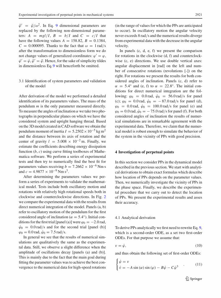
ϕ′ = ϕ/ω2. In Eq. 9 dimensional parameters arereplaced by the following non-dimensional parame-ters: A = mgl/I , B = b/I and C = c/I thathave the following values A = 158.82, B = 0.1384,C = 0.000095. Thanks to the fact that ω = 1 rad/safter the transformation to dimensionless form we donot change values of generalized coordinates: ϕ′ = ϕ,ϕ′ = ϕ, ϕ′ = ϕ. Hence, for the sake of simplicity tildesin dimensionless Eq.9 will henceforth be omitted.

3.1 Identification of system parameters and validationof the model

After derivation of the model we performed a detailedidentification of its parameters values. The mass of thependulum m is the only parameter measured directly.Tomeasure the angles of inclinationαwe take two pho-tographs in perpendicular planes on which we have theconsidered system and upright hanging thread. Basedon the 3Dmodel created inCADsoftwarewe obtain thependulummoment of inertia I = 5.2502×10−5 kgm2

and the distance between its axis of rotation and thecenter of gravity l = 5.008 × 10−2 m. Finally, weestimate the coefficients describing energy dissipationfunction (b, c) using curve fitting toolboxes of Mathe-matica software. We perform a series of experimentaltests and then try to numerically find the best fit forparameters values receiving b = 7.2662 × 10−6 Nm sand c = 4.9877 × 10−9 Nm s3.

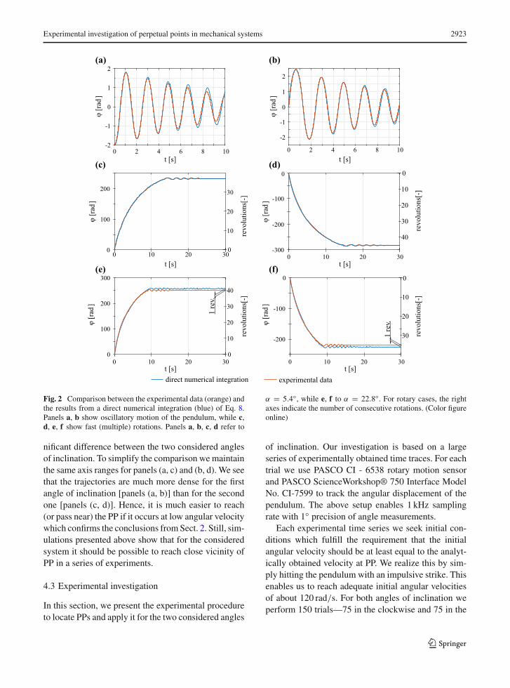
After determining the parameters values we per-form a series of experiments to validate the mathemat-ical model. Tests include both oscillatory motion androtations with relatively high rotational speeds both inclockwise and counterclockwise directions. In Fig. 2we compare the experimental data with the results fromdirect numerical integration of the model. Panels (a, b)refer to oscillatory motion of the pendulum for the firstconsidered angle of inclination (α = 5.4◦). Initial con-ditions for the first trial [panel (a)] were ϕ0 = −2.0 rad,ϕ0 = 0.0 rad/s and for the second trial [panel (b)]ϕ0 = 0.0 rad, ϕ0 = 7.5 rad/s.

In general we see that the results of numerical sim-ulations are qualitatively the same as the experimen-tal data. Still, we observe a slight difference when theamplitude of oscillations decay [panels (a) and (b)].This is mainly due to the fact that the main goal duringfitting the parameter values was to achieve the best con-vergence to the numerical data for high-speed rotations

(in the range of values for which the PPs are anticipatedto occur). In oscillatory motion the angular velocitynever exceeds 8 rad/s and the numerical results divergefrom experimental data with the decrease in the angularvelocity.

In panels (c, d, e, f) we present the comparisonfor rotations in the clockwise (d, f) and counterclock-wise (c, e) directions. We use double vertical axes:angular displacement in [rad] on the left and num-ber of consecutive rotations (revolutions [-]) on theright. For rotations we present the results for both con-sidered angles of inclination. Panels (c, d) refer toα = 5.4◦ and (e, f) to α = 22.8◦. The initial con-ditions for direct numerical integration are the fol-lowing: ϕ0 = 0.0 rad, ϕ0 = 56.0 rad/s for panel(c); ϕ0 = 0.0 rad, ϕ0 = − 87.0 rad/s for panel (d),ϕ0 = 0.0 rad, ϕ0 = 100.0 rad/s for panel (e) andϕ0 = 0.0 rad, ϕ0 = − 75.0 rad/s for panel (f). For bothconsidered angles of inclination the results of numer-ical simulations are in remarkable agreement with theexperimental data. Therefore, we claim that the numer-ical model is robust enough to simulate the behavior ofthe system in the vicinity of PPs with good precision.

4 Investigation of perpetual points

In this section we consider PPs in the dynamical modeldescribed in the previous section.We start with analyti-cal derivations to obtain exact formulas which describehow location of PPs depends on the parameter values.Then, we numerically investigate the vicinity of PPs inthe phase space. Finally, we describe the experimen-tal procedure that we carry out to detect the locationof PPs. We present the experimental results and assestheir accuracy.

4.1 Analytical derivation

To derive PPs analyticallywe first need to rewrite Eq. 9,which is a second-order ODE, as a set two first-orderODEs. For that purpose we assume that:

v = ϕ, (10)

and thus obtain the following set of first-order ODEs:{

ϕ = v

v = −A sin (α) sin (ϕ) − Bϕ − C ϕ3. (11)

123

2922 P. Brzeski, L. N. Virgin

The PPs are given by the following set of equations:⎧⎪⎨⎪⎩

ϕ �= 0

ϕ = 0

v = 0

(12)

Using the above formula we can derive the PPs ana-lytically, resulting in:

⎧⎪⎪⎪⎨⎪⎪⎪⎩

ϕ = (n − 0.5)π

v = B(2/

(−27A sin (α)C2 +

√12B3C3 + 81 (A sin (α))2 C4

))1/3 +−

((−9A sin (α)C2 +

√12B3C3 + 81 (A sin (α))2 C4

)/18

)1/3/C

∈ Z ,

⎧⎪⎪⎪⎨⎪⎪⎪⎩

ϕ = (n + 0.5)π

v = B(2/

(27A sin(α)C2 +

√12B3C3 + 81 (A sin(α))2 C4

))1/3 +−

((9A sin(α)C2 +

√12B3C3 + 81 (A sin(α))2 C4

)/18

)1/3/C

n ∈ Z. ,

(13)

It is important to notice that the system under con-sideration has the following property:...ϕ = 0 ⇔ ϕ(n + 0.5)π n ∈ Z, (14)

and thus the jerk is equal to zero when ϕ = (n+0.5)π .It is a specific feature of the investigated system andstrongly simplifies our analysis.

For the sake of simplicity we assume that ϕ =(ϕ−π)mod 2π and get ϕ ∈ 〈−π, π〉 rad. Then, usingthe above formulas we calculate PPs. For the first con-sidered angle of inclination α = 5.4◦ we obtain:{

ϕ = 0.5π rad

v = − 45.1195 rad/sand

{ϕ = − 0.5π rad

v = 45.1195 rad/s

(15)

and for the second considered angle of inclination α =22.8◦ we get:{

ϕ = 0.5π rad

v = − 80.9247 rad/sand

{ϕ = − 0.5π rad

v = 80.9247 rad/s.

(16)

We see that in this model it is potentially feasible toreach a PP since they appear at much lower angularvelocities than for typical experimental rigs with pen-dula (seeTable 1). Two important elements in achievingthis accessibility was the tilting the axis of the pendu-lum, and adding the plastic strip to increase the drag.These modifications allowed the parameters values to

be adjusted resulting in a dramatic decrease in the angu-lar velocities at PPs.

4.2 Numerical analysis

After deriving the PPs analytically, now we turn tonumerical solutions of theODEs. In Fig. 3we show tra-

jectories of the system near PP. To present the behaviorof the system we use 3D plots with angular displace-ment ϕ, velocity ϕ and acceleration ϕ on abscissa, ordi-nate and applicate, respectively. Hence, we are ableto depict the surface of zero acceleration (gray half-transparent surface). Moreover, due to the fact thatthe zeros of pendulum jerk are constrained to a spe-cific angle (see Eq. 14) we can also simply display thesurface of zero jerk (yellow half-transparent surface).Therefore, the PPsmust occur at the line of intersectionof these two planes and we mark their position with aspecial marker.

Panels (a, b) of Fig. 3 were calculated for the firstconsidered angle of inclination α = 5.4◦. In panel (a)with lines of different colors we show 7 trajectories thatstart from different initial conditions that are given inTable 3 with the corresponding line colors. In Panel (b)we magnify the close neighborhood of the PP. Simi-larly, in panels (c, d) we consider the system assumingthe second angle of inclination α = 22.8◦. In panel (c)we show the trajectory that goes through the PP and 7nearby trajectories (for initial conditions and line colorssee Table 3). In panel (d) we magnify the local neigh-borhood of the PP. In all the panelswith the bold red linewe highlight the trajectory that starts from the PP andwith the bold blue line the trajectory that approachesthe PP.

Analyzing Fig. 3 we see that it is not that difficultto reach the neighborhood of PPs. Still, there is a sig-

123

Experimental investigation of perpetual points in mechanical systems 2923

0 2 4 6 8 10-2

-1

0

1

2

-2

-1

0

1

2

[φ

]dar [φ

]dar

][st ][st

-300

-200

-100

0

[φ

]dar][st

0 10 20 30

200

100

0

[φ

]dar

][st

(a) (b)

(c) (d)

[φ

]d ar

][st][st

(e) (f)

direct numerical integration experimental data

0 10 20 30

300

200

100

0

[φ

]dar

0 2 4 6 8 10

0 10 20 30

0 10 20 30

-200

-100

0

10

20

30

40

0

.ver1

.ver1

10

20

30

40

0

10

20

30

0

]-[snoitulover10

20

30

0

]-[snoitulover

] -[snoi tu lov er

]-[snoi tulov er

Fig. 2 Comparison between the experimental data (orange) andthe results from a direct numerical integration (blue) of Eq. 8.Panels a, b show oscillatory motion of the pendulum, while c,d, e, f show fast (multiple) rotations. Panels a, b, c, d refer to

α = 5.4◦, while e, f to α = 22.8◦. For rotary cases, the rightaxes indicate the number of consecutive rotations. (Color figureonline)

nificant difference between the two considered anglesof inclination. To simplify the comparison wemaintainthe same axis ranges for panels (a, c) and (b, d). We seethat the trajectories are much more dense for the firstangle of inclination [panels (a, b)] than for the secondone [panels (c, d)]. Hence, it is much easier to reach(or pass near) the PP if it occurs at low angular velocitywhich confirms the conclusions fromSect. 2. Still, sim-ulations presented above show that for the consideredsystem it should be possible to reach close vicinity ofPP in a series of experiments.

4.3 Experimental investigation

In this section, we present the experimental procedureto locate PPs and apply it for the two considered angles

of inclination. Our investigation is based on a largeseries of experimentally obtained time traces. For eachtrial we use PASCO CI - 6538 rotary motion sensorand PASCO ScienceWorkshop® 750 Interface ModelNo. CI-7599 to track the angular displacement of thependulum. The above setup enables 1 kHz samplingrate with 1◦ precision of angle measurements.

Each experimental time series we seek initial con-ditions which fulfill the requirement that the initialangular velocity should be at least equal to the analyt-ically obtained velocity at PP. We realize this by sim-ply hitting the pendulum with an impulsive strike. Thisenables us to reach adequate initial angular velocitiesof about 120 rad/s. For both angles of inclination weperform 150 trials—75 in the clockwise and 75 in the

123

2924 P. Brzeski, L. N. Virgin

Fig. 3 3D plots of thetrajectories in the vicinity ofPPs. Panels a, b refer to thefirst considered angle ofinclination α = 5.4◦, whilec, d to α = 22.8◦. Panel b isthe zoom up of panel (a),and panel d is the zoom upof panel (c). In each panelwe show trajectoriesobtained starting from initialconditions given in Table 3

(a)

(b)

(c)

(d)

counterclockwise directions. This give us time traceswhich are then post-processed with Mathematica soft-ware. Finally, we analyze the results and try to estimatethe location of PPs based on the experimental data only.

4.3.1 Post-processing of the acquired data

The angle measurement device provided good preci-sion, with good spatial and temporal resolution. How-

ever, the main problem is that we are only able to trackthe position of the pendulum ϕ in time, while to obtainPPsweneed to analyze the first, the second and the thirdderivative of the angular displacement which causeshuge problems. Because of the discrete nature of theacquired (inevitably slightly noisy) experimental data,the familiar problem of noise amplification on differen-tiation was encountered. That is one of the reasons whytime lag embedding, where instead of calculating the

123

Experimental investigation of perpetual points in mechanical systems 2925

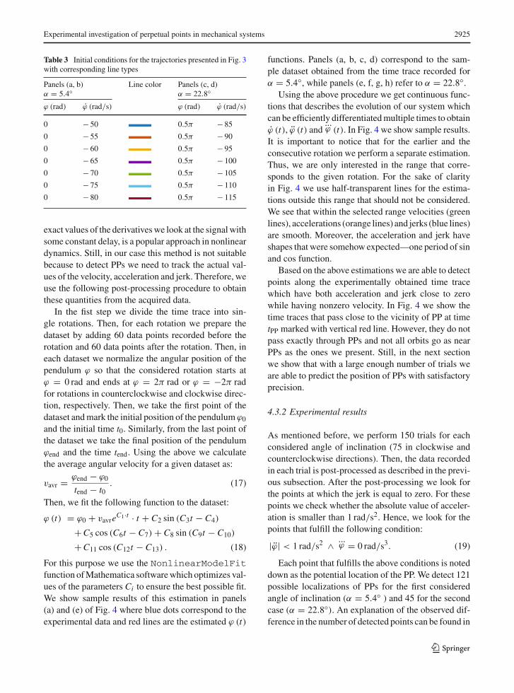
Table 3 Initial conditions for the trajectories presented in Fig. 3with corresponding line types

Panels (a, b) Line color Panels (c, d)α = 5.4◦ α = 22.8◦

ϕ (rad) ϕ (rad/s) ϕ (rad) ϕ (rad/s)

0 − 50 0.5π − 85

0 − 55 0.5π − 90

0 − 60 0.5π − 95

0 − 65 0.5π − 100

0 − 70 0.5π − 105

0 − 75 0.5π − 110

0 − 80 0.5π − 115

exact values of the derivativeswe look at the signalwithsome constant delay, is a popular approach in nonlineardynamics. Still, in our case this method is not suitablebecause to detect PPs we need to track the actual val-ues of the velocity, acceleration and jerk. Therefore, weuse the following post-processing procedure to obtainthese quantities from the acquired data.

In the fist step we divide the time trace into sin-gle rotations. Then, for each rotation we prepare thedataset by adding 60 data points recorded before therotation and 60 data points after the rotation. Then, ineach dataset we normalize the angular position of thependulum ϕ so that the considered rotation starts atϕ = 0 rad and ends at ϕ = 2π rad or ϕ = −2π radfor rotations in counterclockwise and clockwise direc-tion, respectively. Then, we take the first point of thedataset andmark the initial position of the pendulum ϕ0

and the initial time t0. Similarly, from the last point ofthe dataset we take the final position of the pendulumϕend and the time tend. Using the above we calculatethe average angular velocity for a given dataset as:

vavr = ϕend − ϕ0

tend − t0. (17)

Then, we fit the following function to the dataset:

ϕ (t) = ϕ0 + vavreC1·t · t + C2 sin (C3t − C4)

+C5 cos (C6t − C7) + C8 sin (C9t − C10)

+C11 cos (C12t − C13) . (18)

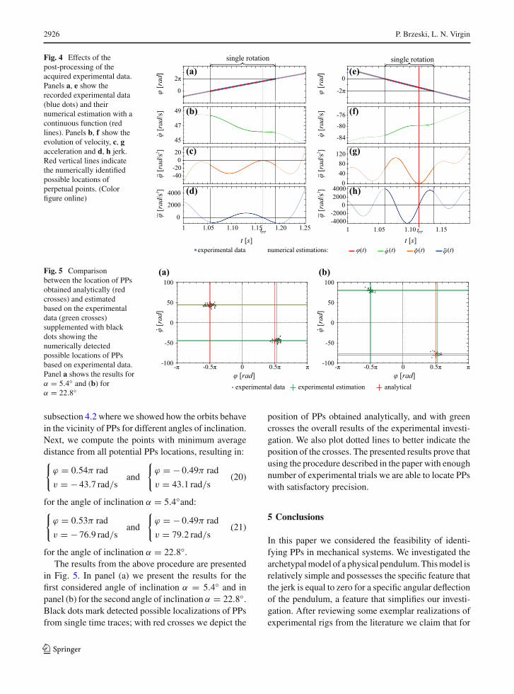
For this purpose we use the NonlinearModelFitfunction ofMathematica softwarewhich optimizes val-ues of the parameters Ci to ensure the best possible fit.We show sample results of this estimation in panels(a) and (e) of Fig. 4 where blue dots correspond to theexperimental data and red lines are the estimated ϕ (t)

functions. Panels (a, b, c, d) correspond to the sam-ple dataset obtained from the time trace recorded forα = 5.4◦, while panels (e, f, g, h) refer to α = 22.8◦.

Using the above procedure we get continuous func-tions that describes the evolution of our system whichcan be efficiently differentiatedmultiple times to obtainϕ (t), ϕ (t) and

...ϕ (t). In Fig. 4 we show sample results.

It is important to notice that for the earlier and theconsecutive rotation we perform a separate estimation.Thus, we are only interested in the range that corre-sponds to the given rotation. For the sake of clarityin Fig. 4 we use half-transparent lines for the estima-tions outside this range that should not be considered.We see that within the selected range velocities (greenlines), accelerations (orange lines) and jerks (blue lines)are smooth. Moreover, the acceleration and jerk haveshapes that were somehow expected—one period of sinand cos function.

Based on the above estimations we are able to detectpoints along the experimentally obtained time tracewhich have both acceleration and jerk close to zerowhile having nonzero velocity. In Fig. 4 we show thetime traces that pass close to the vicinity of PP at timetPP marked with vertical red line. However, they do notpass exactly through PPs and not all orbits go as nearPPs as the ones we present. Still, in the next sectionwe show that with a large enough number of trials weare able to predict the position of PPs with satisfactoryprecision.

4.3.2 Experimental results

As mentioned before, we perform 150 trials for eachconsidered angle of inclination (75 in clockwise andcounterclockwise directions). Then, the data recordedin each trial is post-processed as described in the previ-ous subsection. After the post-processing we look forthe points at which the jerk is equal to zero. For thesepoints we check whether the absolute value of acceler-ation is smaller than 1 rad/s2. Hence, we look for thepoints that fulfill the following condition:

|ϕ| < 1 rad/s2 ∧ ...ϕ = 0 rad/s3. (19)

Each point that fulfills the above conditions is noteddown as the potential location of the PP. We detect 121possible localizations of PPs for the first consideredangle of inclination (α = 5.4◦ ) and 45 for the secondcase (α = 22.8◦). An explanation of the observed dif-ference in the number of detected points can be found in

123

2926 P. Brzeski, L. N. Virgin

Fig. 4 Effects of thepost-processing of theacquired experimental data.Panels a, e show therecorded experimental data(blue dots) and theirnumerical estimation with acontinuous function (redlines). Panels b, f show theevolution of velocity, c, gacceleration and d, h jerk.Red vertical lines indicatethe numerically identifiedpossible locations ofperpetual points. (Colorfigure online)

0

2π

1.05 1.10 1.151

φ]

[dar

t s[ ]

-80

-76

-84φ]s /

[dar

040φ

]s/[dar

0

φ]s/

[dar

801202

3

20004000

-4000-2000

0

-2π

1

t s[ ]

47

49

45

0

-40

0

-20

20

2000

4000

1.05 1.10 1.15 1.20 1.25

single rotationsingle rotation

experimental data φ( )t φ( )tnumerical estimations: φ( )t φ( )t

(a)

(b)

(c)

(d)

(f)

(g)

(h)

tPP tPP

φ]

[dar

φ]s/

[dar

φ] s/

[dar

φ]s/

[dar

23

(e)

Fig. 5 Comparisonbetween the location of PPsobtained analytically (redcrosses) and estimatedbased on the experimentaldata (green crosses)supplemented with blackdots showing thenumerically detectedpossible locations of PPsbased on experimental data.Panel a shows the results forα = 5.4◦ and (b) forα = 22.8◦

0 0.5π π-π -0.5π

0

50

100

-50

-100

φ [ ]rad φ [ ]rad

φ]

[dar

experimental data analyticalexperimental estimation

(a) (b)

0 0.5π π-π -0.5π

0

50

100

-50

-100

φ]

[da r

subsection 4.2 where we showed how the orbits behavein the vicinity of PPs for different angles of inclination.Next, we compute the points with minimum averagedistance from all potential PPs locations, resulting in:{

ϕ = 0.54π rad

v = − 43.7 rad/sand

{ϕ = − 0.49π rad

v = 43.1 rad/s(20)

for the angle of inclination α = 5.4◦and:{

ϕ = 0.53π rad

v = − 76.9 rad/sand

{ϕ = − 0.49π rad

v = 79.2 rad/s.(21)

for the angle of inclination α = 22.8◦.The results from the above procedure are presented

in Fig. 5. In panel (a) we present the results for thefirst considered angle of inclination α = 5.4◦ and inpanel (b) for the second angle of inclination α = 22.8◦.Black dots mark detected possible localizations of PPsfrom single time traces; with red crosses we depict the

position of PPs obtained analytically, and with greencrosses the overall results of the experimental investi-gation. We also plot dotted lines to better indicate theposition of the crosses. The presented results prove thatusing the procedure described in the paper with enoughnumber of experimental trials we are able to locate PPswith satisfactory precision.

5 Conclusions

In this paper we considered the feasibility of identi-fying PPs in mechanical systems. We investigated thearchetypalmodel of a physical pendulum.Thismodel isrelatively simple and possesses the specific feature thatthe jerk is equal to zero for a specific angular deflectionof the pendulum, a feature that simplifies our investi-gation. After reviewing some exemplar realizations ofexperimental rigs from the literature we claim that for

123

Experimental investigation of perpetual points in mechanical systems 2927

most cases PPs occur at high velocities and would beextremely difficult to reach experimentally. Neverthe-less, we propose the design of a simple experimentalrig with a pendulum in which we are able to reducevelocity at PPs, and reach them in a series of experi-ments.

We obtained this characteristic by tilting the rota-tional axis of the pendulum and adding the plastic stripto increase the drag and enhance the energy dissipa-tion. For this specific type of physical pendulum weestablished PPs analytically, numerically and experi-mentally assuming two different angles of tilt. We pro-vided an analytical derivation of PPs and show numer-ical results that reveal how trajectories behave in thevicinity of PPs and in addition show how parametervalues affect the probability of reaching the PP.

The results presented reveal the possible utilizationof PPs which can be used to identify energy dissipationmodels. It is a by-product of the performed investi-gation that we will expand and further analyze in anupcoming paper.

In the final part, we described the experimentalinvestigation undertaken to verify the existence andpractical accessibility of PPs. To obtain velocities,accelerations and jerks from raw experimental data weused a specific post-processing procedure that success-fully eliminated noise and estimated the evolution ofthe system with piece-wise continuous functions. Theresults prove that the proposed procedure is robust andallows an effective estimate of PPs from raw experi-mental data with good precision.

Acknowledgements P. Brzeski is supported by the Foundationfor Polish Science (FNP).

Open Access This article is distributed under the terms of theCreative Commons Attribution 4.0 International License (http://creativecommons.org/licenses/by/4.0/), which permits unrestr-icted use, distribution, and reproduction in any medium, pro-vided you give appropriate credit to the original author(s) andthe source, provide a link to the Creative Commons license, andindicate if changes were made.

References

1. Prasad, A.: Existence of perpetual points in nonlineardynamical systems and its applications. Int. J. Bifurc. Chaos25(02), 1530005 (2015)

2. Prasad, A.: A note on topological conjugacy for perpetualpoints. Int. J. Nonlinear Sci. 21(1), 60–64 (2015)

3. Dudkowski, D., Prasad, A., Kapitaniak, T.: Perpetual pointsand hidden attractors in dynamical systems. Phys. Lett. A379(40), 2591–2596 (2015)

4. Dudkowski, D., Jafari, S., Kapitaniak, T., Kuznetsov, N.V.,Leonov, G.A., Prasad, A.: Hidden attractors in dynamicalsystems. Phys. Rep. 637, 1–50 (2016)

5. Kuznetsov,N.V.:Hidden attractors in fundamental problemsand engineering models: a short survey. In: Duy, V., Dao, T.,Zelinka, I., Choi, H.S., Chadli, M. (eds.) AETA 2015: recentadvances in electrical engineering and related sciences, pp.13–25. Springer, Berlin (2016)

6. Leonov,G.A., Kuznetsov,N.V., Vagaitsev, V.I.: Localizationof hidden Chua’s attractors. Phys. Lett. A 375(23), 2230–2233 (2011)

7. Kuznetsov,A.P.,Kuznetsov, S.P.,Mosekilde, E., Stankevich,N.V.: Co-existing hidden attractors in a radio-physical oscil-lator system. J. Phys. AMath. Theor. 48(12), 125101 (2015)

8. Pham,V.T., Vaidyanathan, S., Volos, C.K., Jafari, S.: Hiddenattractors in a chaotic system with an exponential nonlinearterm. Eur. Phys. J. Spec. Top. 224(8), 1507–1517 (2015)

9. Chaudhuri, U., Prasad, A.: Complicated basins and the phe-nomenon of amplitude death in coupled hidden attractors.Phys. Lett. A 378(9), 713–718 (2014)

10. Brzeski, P., Lazarek, M., Kapitaniak, T., Perlikowski, P.:Basin stability approach for quantifying responses of mul-tistable systems with parameters mismatch. Meccanica51(11), 2713–2726 (2016)

11. Brzeski, P., Wojewoda, J., Kapitaniak, T. Kurths, J., Per-likowski, P.: Sample-based approach can outperform theclassical dynamical analysis—experimental confirmation ofthe basin stability method. Sci. Rep. 7, 6121 (2017)

12. Nazarimehr, F., Saedi, B., Jafari, S., Sprott, J.C.: Are per-petual points sufficient for locating hidden attractors? Int. J.Bifurc. Chaos 27(03), 1750037 (2017)

13. Dudkowski, D., Prasad, A., Kapitaniak, T.: Perpetual points:new tool for localization of coexisting attractors in dynam-ical systems. Int. J. Bifurc. Chaos 27(04), 1750063 (2017)

14. Pham, V.T., Volos, C., Jafari, S., Kapitaniak, T.: Coexistenceof hidden chaotic attractors in a novel no-equilibrium sys-tem. Nonlinear Dyn. 87(3), 1–10 (2016)

15. Jiang, H., Liu, Y., Wei, Z., Zhouchao, L.: Hidden chaoticattractors in a class of two-dimensional maps. NonlinearDyn. 85(4), 2719–2727 (2016)

16. Pham, V.T., Volos, C., Jafar, S., Kapitaniak, T.: Coexistenceof hidden chaotic attractors in a novel no-equilibrium sys-tem. Nonlinear Dyn. 87(3), 2001–2010 (2017)

17. Wei, Z., Pham, V.T., Kapitaniak, T., Wang, Z.: Bifurcationanalysis and circuit realization for multiple-delayed wang-chen system with hidden chaotic attractors. Nonlinear Dyn.85(3), 1635–1650 (2016)

18. Leonov, G.A., Kuznetsov, N.V., Mokaev, T.N.: Homoclinicorbits, and self-excited and hidden attractors in a Lorenz-like system describing convective fluid motion. Eur. Phys.J. Spec. Top. 224(8), 1421–1458 (2015)

19. Jafari, S., Nazarimehr, F., Sprott, J.C., Golpayegani,S.M.R.H.: Limitation of perpetual points for confirmingconservation in dynamical systems. Int. J. Bifurc. Chaos25(13), 1550182 (2015)

20. Nazarimehr, F., Jafari, S., Golpayegani, S.M.R.H., Sprott,J.C.: Categorizing chaotic flows from the viewpoint of fixed

123

2928 P. Brzeski, L. N. Virgin

points and perpetual points. Int. J. Bifurc. Chaos 27(02),1750023 (2017)

21. Ueta, T., Ito, D., Aihara, K.: Can a pseudo periodic orbitavoid a catastrophic transition? Int. J. Bifurc. Chaos 25(13),1550185 (2015)

22. de Paula, A.S., Savi, M.A., Pereira-Pinto, F.H.I.: Chaos andtransient chaos in an experimental nonlinear pendulum. J.Sound Vib. 294(3), 585–595 (2006)

23. Zilletti, M., Elliott, S., Ghandchi Tehrani, M.: Electrome-chanical pendulum for vibration control and energy harvest-ing In: EACS 2016—6th European conference on structuralcontrol at Sheffield, England (2016)

24. Kecik, K., Brzeski, P., Perlikowski, P.: Non-linear dynam-ics and optimization of a harvester–absorber system. Int. J.Struct. Stab. Dyn. 17(5), 1740001 (2016)

25. George, C., Virgin, L.N., Witelski, T.: Experimental studyof regular and chaotic transients in a non-smooth system.Int. J. Non-Linear Mech. 81, 55–64 (2016)

26. Lenci, S., Rega, G.: Experimental versus theoretical robust-ness of rotating solutions in a parametrically excited pendu-lum: a dynamical integrity perspective. Phys. D NonlinearPhenom. 240(9), 814–824 (2011)

27. Marszal, M., Witkowski, B., Jankowski, K., Perlikowski, P.,Kapitaniak, T.: Energy harvesting from pendulum oscilla-tions. Int. J. Non-Linear Mech. 94, 251–256 (2017)

123