Experimental facility dedicated to high temperatures...

Experimental facility dedicated to high temperature thermophysical properties measurement: validation of the temperature measurement by multispectral method

by L. Dejaeghere* **, T. Pierre*, M. Carin*, P. Le Masson*

* Univ. Bretagne-Sud, EA 4250, LIMATB, Rue de Saint Maudé, 56100 Lorient, France ** IRT JULES VERNE, Chemin du Chaffault, 44340 Bouguenais, France

Abstract

The knowledge of physical properties of metals above their melting point is essential regarding the numerical

simulation of welding processes. The measurement of these properties requires a device able to heat a small sample up to 2 000 °C and an appropriate temperature measurement apparatus. This paper presents the development of an induction heating furnace which will be used to measure thermophysical properties of metallic samples, and an optical pyrometer composed of a five colors (visible and NIR) dedicated to steady-state and dynamic measurements. The optical bench is tested up to 1 200 °C using multiple classical bichromatic pyrometry. 1. Introduction

Welding process simulation requires the knowledge of high temperature thermophysical properties. It is quite common to find these properties up to near the melting point of the material [1, 2], nevertheless, the data around and above the melting point are scarce.

Some studies in literature give some insight about metal properties such as thermal conductivity and diffusivity [3], specific heat, density, surface tension [4]… Boivineau et al. summarize in [5] different methods of high temperature from millisecond measurement to submicrosecond measurement.

The methods described in [5] are used on metal rods heated up by joule effect for different periods of time. Millisecond methods are used up to 3 000 °C for the determination of thermal and electric properties. Nevertheless, measurements are limited to solid state due to the collapsing of the rod. Microsecond methods are used from 2 000 up to 10 000 °C, they allow measurements of liquid metal since the collapsing time of the rod is longer than the measurement time. Submicrosecond measurements are dedicated to explosion experiments. However, those measurements are disturbed by electrical and hydrodynamic instabilities.

The difficulties of such measurements are mainly due to control over heat and chemical transfers (problem of diffusion). A way to avoid these difficulties is to use electromagnetic levitation like it was done in [4, 6]. Doing so imply as well few difficulties like the stabilization of the sample shape and the creation of interne fluid movements by the electromagnetic field.

Whatever the method is, temperature knowledge is essential to these kinds of measurements. Thermocouples may be used but it is an intrusive method and they are limited by their range of temperature [7]. It is possible to place thermocouples in colder places but it drives it away from the investigated area, which lead to an increase of the measurement uncertainty. A non-invasive method is to use pyrometer, which is an interesting alternative for high temperatures, but a knowledge of the material emissivity is necessary [8]. Emissivity is a physical property dependent of temperature, direction, wavelength and roughness [1-2, 9]. A classical way to solve this lack of knowledge is to use a multispectral method which consists of simultaneous measurements for the same surface at different wavelengths [10]: these combined measurements allow retrieving temperature and emissivity at the same time [11]. In any case, for high temperature, oxidation of the sample will influence the material emissivity and disturb the measurement [12].

This paper presents the size and design of an experimental device able to heat up samples to 2 000 °C, and its temperature measurement device. The dimensioning will be treated in three parts.

First, this article presents a presentation of the heating system which includes the heat source, the materials used and their physical properties used for the numerical simulation and an enumeration of the instrumentation for temperature measurement.

Second, the results of a numerical simulation done thanks to Comsol multiphysics® is presented. This part includes a presentation of the different physics used and their equations, their application domains and a discussion about the results of the numerical study itself.

Third, this article develops the temperature measurement of the sample thanks to multispectral measurements. This part includes a brief reminder about multispectral measurements, results of a blackbody calibration.

http://dx.doi.org/10.21611/qirt.2014.158

2. The high temperature experimental device

2.1. Description of the experimental device

The idea is to develop a device able to heat

metallic samples up to 2 000 °C or more. A 24 kW induction furnace has been chosen as heat source with working frequency set at 105 kHz and constant power during the whole heating process. Figure 1 presents the high temperature device simulated in an axisymmetric geometry. The sample is set in a crucible made of R4550 graphite (1) at the center of the device. The induction (2) system heats the graphite, but in order to favor radiative and conductive heating, the diameter of the graphite has been dimensioned in order to avoid magnetic fields in the crucible. The top and the bottom faces of the graphite R4550 are thermally isolated thanks to graphite GFA12 (3). The insulating material is placed upon Stumatite® (4), a refractory material. Moreover, heating graphite to 2 000 °C requires to work under neutral atmosphere. Therefore, it is placed in a vacuum chamber (5) of aluminum 5083 (AISI). The inductor is brought in through a cable gland in order to ensure the seal. This cable gland is water-cooled.

The temperature of the device is controlled by two different ways: type C thermocouples and a pyrometer. Even if they are limited to about 2 300 °C, type C thermocouples must be placed in regions where they cannot be damaged and influenced by electromagnetic field. If some thermocouples are used to get experimental data, one is for the induction regulation. The second way to control temperature is the pyrometry. It is based on the radiative flux measurement. Experimentally this measurement is made possible thanks the vacuum chamber which has a sapphire window on its top (6), which is also water-cooled. Thus the pyrometer is placed on top and collects the radiative flux emitted from the specimen through this window. The pyrometer is described further in this article.

Figure 1: presentation of the high temperature experimental device.

2.2. Simulation of the experimental device

In order to validate experimental choices, a numerical simulation has been done using the software Comsol

Multiphysics®. Two equations are solved: electromagnetic and heat transfer equations. The power of the induction device is set manually and is constant during the whole heating process. If we assume also that the electromagnetic properties are constant, the heat source generated by the induction can be calculated solving only the electromagnetism equations. The heat transfer equation is then solved using the calculated heat source. This weak coupling in association with a 2D axisymmetric assumption has the advantage to reduce computation time.

2.3. Governing equations

The Maxwell electromagnetic equations used for the simulation are given by Eqs. (1) to (4) where B is the magnetic flux density in T, A the magnetic potential vector in T.m-1, µ the relative permeability, H the magnetic field intensity in A.m-1, E the electric field V.m-1, the imaginary number, the pulsation in Hz, the electric flux density V.m-1, the relative permittivity, the current density associated to the free charges in A.m-2.

µ (1)

(2)

(3)

(4)


The local ohm law is expressed by Eq. (5) where is the electrical conductivity of the material in S.m-1 and the current density associated to charges exterior to the model A.m-2.

(5)

Equations (4) and (5) combined together gives:

(6)

Then replacing H using Eq. (1), E using Eq. (2) and D using Eq. (3) gives the following equation:

(

)

(7)

Finally with Eq. (1) to replace B and Eq. (2) to replace E, the formulation used in the presented model is:

( ) (

) (8)

Considering now the equations used for heat transfer, the energy conservation equation is:

( ) (9)

Where is the density (kg·m-3), the specific heat capacity (J·kg-1·K-1), T the temperature (K), k the thermal conductivity (W.m-1.K-1) and Q the joule heating effect created by the induced current in W.m-3. The boundary condition at a solid-gas interface is governed by the following equation:

( ) [ ( )] (10)

With the outward normal vector of the surface at a solid-gas interface, the thermal conductivity in W.m-1.K-1, F the view factor, the emissivity, the incoming flux radiation in W.m-2 and ( ) the black body radiation in W.m-2.

It should be mentioned that the gas inside the chamber is assumed to be static, so no convection is considered in this first model. These equations are solved using the thermophysical properties summarized in Appendix. The material data are taken from literature or supplier database.

2.4. Numerical model

The electromagnetic part is calculated with a 105 kHz frequency and surface current over the external part of the spires. The outer part of the aluminum chamber is modeled as magnetically isolated. Concerning the boundary conditions for the heat transfer problem, radial and convective losses are applied at the outer boundary of the aluminum chamber with a convective heat transfer of 10 W·m-2·K-1

and an emissivity given in Appendix. The temperature on the top of the chamber is set to 20 °C to represent the effect of a water-cooling device. The temperature inside the spires of the inductor is set to 20°C thus modeling the water-cooling system of the inductor. The water inside the spires is not meshed.

The R4550 graphite is heated by the heat source calculated previously in the electromagnetic problem. The heat is then diffused by conduction to the GFA12. The GFA12 has been designed in order to limit heat losses both by conduction to the Stumatite and by radiation to the aluminum walls. This sizing improves the maximal temperature possible for the device.

The solver used for calculation is a parallel sparse direct solver called MUMPS by Comsol Multiphysics®. An adaptive time stepping is used with the BDF method.

For these simulations, the sample is not represented so the sample chamber is filled only with argon. It is shown that magnetic field in the sample chamber can be neglected since its maximum value is under half of the terrestrial magnetic. The hypothesis of magnetically isolated wall is also validated since the residual magnetic field inside the walls is less than 1 µT. In figure 3, the simulation shows that the temperature is stabilized in the sample chamber over two and a half hours, while the temperature in the whole model takes about 4 hours to be fully stabilized. Once the sample chamber is stabilized, it is observed that the temperature difference in the chamber does not exceed 5 °C at 2 000°C. These remarks show that it is possible to consider that the sample has a homogenous temperature and is not disturbed by magnetic fields.

The device is still in progress, so the numerical results will be compared to experimental data in a future work. A comparison with thermocouple measurements will be performed in the limit of their reliability. Another temperature


measurement will be done at the same time through a multispectral pyrometer, presented in the next section. This measurement will be first calibrated using thermocouples measurement and materials with well-known melting point.

The main objective of this first model is to guarantee the homogeneity of the sample chamber and avoid the over heat of the aluminum walls. The convection inside the aluminum and the sample chambers is neglected here. The next paragraph will show the influence of this strong hypothesis in the calculated results. First, convection tends to homogenize the temperature. However, the calculation shows that the temperature is already homogenized inside the sample chamber, so the results in this area are not affected. Second, outside the sample chamber but still inside the aluminum chamber, convection stirs up the heat towards the top. Since convection is not calculated inside the aluminum chamber, the simulation underestimates the temperature in the upper wall while overestimating the temperature in the bottom wall. Assuming that the water-cooled system of the upper wall is efficient enough, the effects of convection on the upper wall is negligible. However, there is still a non-negligible part of convection is on the bottom wall of the aluminum chamber. Nevertheless, while overestimating the temperature, the results show that the bottom wall does not heat over 60°C, which means that no other specific cooling is required for that part.

Figure 2: magnetic and thermal results of the numerical simulation around the sample chamber

Figure 3: simulated temperature of the center of the sample chamber

3. Optical bench

The optical bench has been developed in order to realize steady-state and fast transient measurements of radiative flux for an estimation of the temperature and the emissivity. The non-invasive multispectral pyrometer is used as a complement of the thermocouple measurement. Experimentally this device looks at the sample through a sapphire window placed upon the aluminum chamber (see Figure 1). The pyrometer is positioned thanks to a 4-axis (x, y, , ) platform. The development of the optical bench implies the choice on one hand of a number of wavelengths and on the other hand of the spectral range.

3.1. Multispectral measurements

The treatment of radiative fluxes measured at multiple wavelengths, known as Multispectral method, is used to determine the temperature T and/or the emissivity ( ) of a surface. Assuming the Wien approximation , the theoretical flux

for a wavelength arriving to a sensor can be written as Eq. (11) where ( ) is a transfer function. ( ) can be determined by calibration with a blackbody.

( ) ( )

(11)

() can be a function of several parameters (Drude’s law [13], polynomial function…). Rodiet et al. in [14] remind that two approaches are possible to realize the estimations. The first is based on the fluxes ratio and Wien approximation, which gives an expression of the temperature Tij from two fluxes

and (12). The objective is to find

the values of T and () by minimizing the following cost function JT (13).

(

)

[

( )

( ) ( )

( )( )

]

(12)


[ ( )] ∑| [ ( )]|

(13)

The second approach consists in working directly with the fluxes instead of the temperatures in the new cost function J (14).

[ ( )] ∑|

[ ( )]|

(14)

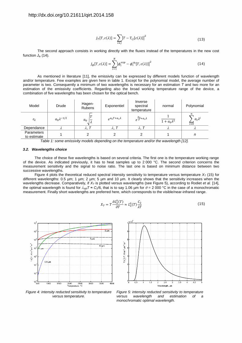
As mentioned in literature [11], the emissivity can be expressed by different models function of wavelength and/or temperature. Few examples are given here in table 1. Except for the polynomial model, the average number of parameter is two. Consequently a minimum of two wavelengths is necessary for an estimation T and two more for an estimation of the emissivity coefficients. Regarding also the broad working temperature range of the device, a combination of five wavelengths has been chosen for the optical bench.

Model Drude Hagen-Rubens Exponentiel

Inverse spectral

temperature normal Polynomial

√

∑

Dependance , T , T , T Parameters to estimate 1 2 2 2 1 n

Table 1: some emissivity models depending on the temperature and/or the wavelength [12].

3.2. Wavelengths choice

The choice of these five wavelengths is based on several criteria. The first one is the temperature working range of the device. As indicated previously, it has to heat samples up to 2 000 °C. The second criterion concerns the measurement sensitivity and the signal to noise ratio. The last one is based on minimum distance between two successive wavelengths.

Figure 4 plots the theoretical reduced spectral intensity sensitivity to temperature versus temperature XT (15) for different wavelengths: 0.5 µm; 1 µm; 2 µm; 5 µm and 10 µm. It clearly shows that the sensitivity increases when the wavelengths decrease. Comparatively, if XT is plotted versus wavelengths (see Figure 5), according to Rodiet et al. [14], the optimal wavelength is found for optT ≈ C2/6, that is to say 1.06 µm for = 2 000 °C in the case of a monochromatic measurement. Finally short wavelengths are preferred here, which corresponds to the visible/near-infrared range.

( )

( )

(15)

Figure 4: intensity reducted sensitivity to temperature

versus temperature. Figure 5: intensity reducted sensitivity to temperature versus wavelength and estimation of a monochromatic optimal wavelength.


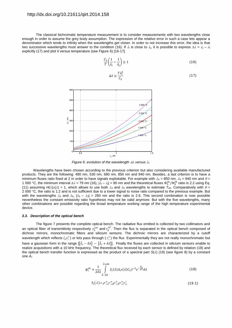
The classical bichromatic temperature measurement is to consider measurements with two wavelengths close enough in order to assume the grey body assumption. The expression of the relative error in such a case lets appear a denominator which tends to infinity when the wavelengths get closer. In order to not increase this error, the idea is that two successive wavelengths must answer to the condition (16). If i is close to j, it is possible to express = j – i explicitly (17) and plot it versus temperature (see Figure 6) [16-17].

(

) (16)

(17)

Figure 6: evolution of the wavelength versus i.

Wavelengths have been chosen according to the previous criterion but also considering available manufactured

products. They are the following: 480 nm, 530 nm, 680 nm, 850 nm and 940 nm. Besides, a last criterion is to have a minimum fluxes ratio fixed at 2 in order to have signals exploitable. For example with 4 = 850 nm, 5 = 940 nm and = 1 000 °C, the minimum interval = 79 nm (16), |i – j| = 90 nm and the theoretical fluxes ratio is 2.2 using Eq. (11) assuming H()() = 1, which allows to use both 4 and 5 wavelengths to estimate T45. Comparatively with = 2 000 °C, the ratio is 1.2 and is not sufficient due to a lower signal to noise ratio compared to the previous example. But with the wavelengths 3 and 5, |5 – 3| = 260 nm and the ratio is 2.6. This second combination is now possible nevertheless the constant emissivity ratio hypothesis may not be valid anymore. But with the five wavelengths, many other combinations are possible regarding the broad temperature working range of the high temperature experimental device. 3.3. Description of the optical bench

The figure 7 presents the complete optical bench. The radiative flux emitted is collected by two collimators and an optical fiber of transmittivity respectively

and . Then the flux is separated in the optical bench composed of

dichroic mirrors, monochromatic filters and silicium sensors. The dichroic mirrors are characterized by a cutoff wavelength which reflects ( m

) or lets pass through ( m

) the flux. Experimentally they are not really monochromatic but have a gaussian form in the range [[ ] [ ]]. Finally the fluxes are collected in silicium sensors enable to realize acquisitions with a 10 kHz frequency. The theoretical flux received by each sensor is defined by relation (18) and the optical bench transfer function is expressed as the product of a spectral part S() (19) (see figure 8) by a constant one Ai.

∫ ( ) ( )

(18)

1 4 3 2 1 1

m m m m fS (19.1)


2 4 3 2 1 2

m m m m fS (19.2)

3 4 4 3 3

m m m fS (19.3)

4 4 3 4

m m fS (19.4)

5 4 5

m fS (19.5)

Experimentally, the first measurements are based on the temperature estimation by bichromatic method. A

calibration has been realized in order to estimate a geometrical ratio coefficient Gij = Ai/Aj (18) and (20) for each case with a blackbody between 700 °C and 1 700 °C. An accurate knowledge of Gij is essential to perform an accurate estimation of the temperature Tij. Eq. (20) describes the relation between T, the blackbody temperature, and

, the fluxes measured by the sensors.

Figure 9 presents the calculation of each Gij versus temperature, which will be used for the further experimental measurements. It appears on one hand that every Gij tends to a constant value and on the other hand that there is a minimum temperature of using the sensors. For example, any combination with the 480 nm wavelength will not be relevant under 1600 °C. The ration Signal/noise is too low for this particular wavelength under 1600 °C.

Figure 9 : Coefficient Gij versus temperature.

Figure 7: description of the optical bench.

Figure 8: representation of the spectral parts S() of the optical bench transfer function.

( )

( )

(20)


3.4. Experimental measurements

The optical bench has been tested independently using a Gleeble® 3500 machine dedicated to

thermomechanical characterization of metals (see Figure 10). The tested metallic specimen, a tungsten plate of dimensions 150 × 30 × 0.05 mm3

, is resistively heated. Four thermocouples are welded on one face to the specimen according to the following positions: z = 0: TC1; z = ± 10 mm: TC2 and TC3; z = 30 mm: TC4. However, due to the nature of the sample and its thickness, only two of them stayed correctly (TC1 and TC2). The pyrometer focuses on a 20 mm diameter surface situated on the opposite face of the sample. The thermocouple TC2 is also used to control the electrical input in the specimen. Static and dynamic (10 °C·s-1) evolutions of temperature are programmed and integration time is of 100 ms. It is also possible to control the machine environment to get rid of the surface oxidation problem but the presented experimentation is under air condition.

Figure 10: presentation of the experimental device using the Gleeble® 3500 machine.

The results are presented in Figure 11 and in table 2. One can notice that a part of the difference between

bichromatic and thermocouple measurement is a constant. This constant can be physically explained by the hypothesis made in birchromatic measurements of a constant emissivity at the two considered wavelength. If this hypothesis is not validated, then a constant error is added to the temperature measurement. There is two ways possible to correct this error. The first one is to recalibrate the measurement while measuring, with the known melting point of the sample for example. The second one is to use multiwavelengths technics which allow to measure temperature and emissivity at the same time.

Figure 11: temperature measurements of a tungsten sample in Gleeble

®

TC1 TC2 T54 2.8% 3.8% T53 1.85% 0.95% T43 2.3% 1.4%

Table 2: mean temperature measurement difference between thermocouples and bichromatic

measurements


3.5. Conclusion on multiwavelength measurements

While calibration with a black body allows measurements within a precision of 2.8 %, an improved measurement

is possible. In order to do so, it is important to recalibrate the pyrometer at each experience. In our case, one way to do so is to use thermocouples within their temperature range or use the melting point of the sample as a temperature marker. The last option is only possible with a slow temperature around the melting point. The experimental device presented at the beginning of this article is able to do both at the same time. Thanks to it, it will be possible to have a double calibration of the measurement and ensure a multiwavelengths measurement with less than 1% error. 4. Conclusions

A high temperature furnace has been dimensioned. The numerical simulation of it shows a homogenous temperature inside the sample chamber over 2 000 °C and a negligible residual magnetic field in a stationary state. These results indicate fluid mechanical physic can be negligible inside the sample. In parallel, the temperature measurement of the sample has been validated within a 3% error and can be improved to drop the error measurement to less than 1%.

The numerical simulation of the high temperature furnace still needs to be confronted to reality thanks to some measurements. Once this step done, the device will be ready to be instrumented for flash method measurement of thermal properties. 5. Acknowledgements

The authors would like to acknowledge the IRT JULES VERNE and the Brittany region for the financial support

provided.

REFERENCES

[1] F. P. Incropera et al., Fundamentals of heat and mass transfer, John Wiley & Sons, New-York, 2002. [2] Y.S. Touloukian, Thermal radiative properties, Plenum, New York, 1970. [3] S. Mehmood et al., Modeling of Effective Thermal Conductivities of Alloy Series as a Function of Temperature in

the Liquid Region, Proceeding of the 18th symposium on thermophysical properties, Boulder, CO, USA, June 24-29. 2012.

[4] G. Wille et al., Thermophysical Properties of Containerless Liquid Iron up to 2500 K, International Journal of Thermophyisics, Vol. 23, No. 5, September 2002.

[5] M. Boivineau et al., Thermophysical properties of metals at very high temperatures obtained by dynamic heating techniques: recent advances, Int. J. Materials and Product Technology, Vol. 26, Nos 3/4, 2006.

[6] M. Watanabe et al., Measurements of Density and Structure of Alloys Liquids by Levitation Technique, Proceeding of the 18th symposium on thermophysical properties, Boulder, CO, USA, June 24-29. 2012.

[7] J.-P. Bardon, B. Cassagne, Température de surface, mesure par contact, Techniques de l’ingénieur, r2730. [8] H. R. B. Orlande et al., Thermal measurements and inverse techniques, CRC Press, Taylor and Francis, Boca

Raton, 2011. [9] R. Siegel, J. Howell, Thermal radiation heat transfer, 4th Ed. Taylor & Francis, New-York, 2002. [10] T. Pierre et al., Micro-scale temperature by multi-spectral and statistic method in the UV-visible wavelengths, J.

Appl. Phys. 103(3), p.1-10, 2008. [11] T. Duvaut et al., Multiwavelength infrared pyrometry: optimization and computer simulations, Infrared Physics &

Technology 36 (1995) 1089-1103. [12] K.-H. Weng et al., Effect of oxidation on aluminium alloys temperature prediction using radiation thermometry,

International Journal of Heat and Mass Transfer 54 (2011) 4834-4843. [13] J. Taine, J.-P. Petit, Transferts thermiques anisothermes, Ed. Dunod, Paris, 1998. [14] C. Rodiet et al., Optimisation of wavelength selection used for the multi-spectral temperature measurement by

ordinary least squares method of surfaces exhibiting non-uniform emissivity, Quantitative Infrared Thermography, 10(2), p. 222-236, 2013.

[15] T. Pierre, Mesure de la températureà l’échelle microscopique par voie optique dans la gamme ultraviolet-visible, thèse de doctorat, Nancy-Université, 2007.

[16] J. Thevenet, M. Siroux, B. Desmet, Measurements of brake disc surface temperature and emissivity by two-color pyrometry, Applied Thermal Engineering 30 (2010) 753-759.


APPENDIX

Graphite R4550 Graphite GFA Stumatite Aluminum argon copper

Density (kg.m-3)

From 293 to 2273 :

From 293 to 2273 :

2650

From 100 to 575 : a1 = 1,007.10-12

a2 = -2,270.10-9

a3 = 2,004.10-6

a4 = -9,256.10-4

a5 = 3,368.10-2

a6 = 2699,543

From 87 to 3000 :

From 250 to 1250 : a1 = -8,730.10-5

a2 = -3,926.10-1

a3 = 9062,604

Thermal conductivity (W.m-1.K-1)

From 293 to 2273 : 0.32T+322.64

From 293 to 2273 : a1 = -1,197.10-14

a2 = 7,686.10-11

a3 = -1,875.10-7

a4 = 2,433.10-4

a5 = -2,218.10-1

a6 = 1,559

1,4

From 273 to 849 : a1 = 3,182.10-7

a2 = -6,570.10-4

a3 = 4,662.10-1

a4 = 30,016

From 88 to 340 : a1 = 2,864410-11

a2 = -5,020.10-8

a3 = 7,233.10-5

a4 = -2,420.10-4

From 340 to 690 : a1 = 2,097.10-11

a2 = -5,225.10-8

a3 = 7,367.10-5

a4 = -2,467.10-4

From 690 to 2500 : a1 = -1,587.10-15

a2 = 1,050.10-11

a3 = -2,632.10-8

a4 = 5,576.10-5

a5 = 4,222.10-3

328

Thermal capacity

(J.kg-1.K-1) 530 530

From 473 to 1273 : a1 = 3,906.10-9

a2 = -1,333.10-5

a3 = 1,601.10-2

a4 = -7,668

a3 = 2,210.103

From 273 to 373 : 520,326

From 273 to 1300 : a1 = 1,140.10-10

a2 = -1,971.10-7

a3 = 5,535.10-5

a4 = 1,338.10-1

a3 = 342,764

Electrical conductivity

(S.m-1)

From 293 to 2273 : a1 = 1,658.10-5

a2 = -9,269.10-2

a3 = 1,528.102

a4 = 3,790.104

From 293 to 2273 :

From 293 to 1273 : 17.106 1.10-13

From 100 to 1358 :

With :

a1 = 1,026.10-17

a2 = -8,917.10-15

a3 = 7,064.10-11

a4 = -3,514 Relative

permittivity 1 1 1 1 1 1

Relative permeability 15 1,7 1 1 1 1

Annex 1: thermal and electrical properties of the materials composing the high temperature device. The polynomial laws are expressed in the form: ( ) ∑


Experimental facility dedicated to high temperatures...

Documents

Transcript of Experimental facility dedicated to high temperatures...