Experimental Evaluation of Two-Dimensional Media Scaling

Experimental Evaluation of Two-Dimensional Media Scaling Techniques for Internet Videoconferencing

by

Peter A. Nee

A thesis submitted to the faculty of the University of North Carolina at Chapel Hill in partial fulfillment of the

requirements for the degree of Master of Science in the Department of Computer Science.

Chapel Hill

1997

Approved by

______________________________

Advisor: Professor Kevin Jeffay

_____________________________

Reader: Professor Bert Dempsey

______________________________

Reader: Professor F. Donelson Smith

ii

1997

Peter A. Nee

ALL RIGHTS RESERVED

iii

ABSTRACT

Peter A. Nee

Experimental Evaluation of Two-Dimensional Media Scaling Techniques for Internet Videoconferencing

(Under the direction of Kevin Jeffay)

Internet Videoconferencing is a desirable application, but difficult to support as it requires performance

guarantees. However, the Internet is made up of best-effort networks and will be for some time to come. Best-

effort networks are unable to protect distributed, multimedia applications such as videoconferencing from the

effects of congestion. End-to-end adaptive scaling methods allow such applications to operate in the absence of

network service guarantees. This thesis extends previous work on two-dimensional media scaling, a method that

adapts the bit-rate and packet-rate of media streams. We apply two-dimensional scaling to a commercial codec

architecture and evaluate the performance in experiments with live Internet traffic. These experiments show some

benefits to incorporating two-dimensional scaling in an Internet videoconferencing application, and indicate

directions for further work on two-dimensional adaptive methods.

iv

CONTENTS

Page

LIST OF TABLESÉÉÉÉÉÉÉÉÉÉÉÉÉÉÉÉÉÉÉÉÉÉÉÉÉÉÉÉÉÉÉÉÉvi

LIST OF FIGURESÉÉÉÉÉÉÉÉÉÉÉÉÉÉÉÉÉÉÉÉÉÉÉÉÉÉÉÉÉÉÉ.Évii

Chapter

I. The Videoconferencing Problem............................................................................................1

A. Introduction .................................................................................................................1

B. Background..................................................................................................................1

II. Solutions for the Videoconferencing Problem..........................................................................5

A. Resource Reservation.....................................................................................................5

B. Forward Error Correction................................................................................................7

C. Adaptive Media Scaling Methods.....................................................................................8

1. Media Scaling Techniques for Adaptive Methods.............................................................8

2. Two-Dimensional Scaling Framework......................................................................... 10

3. Feasible points of an operating point set....................................................................... 17

4. Heuristics for Adaptation........................................................................................... 20

III. Internet Experiments with a ProShare Implementation of Media Scaling ................................ 25

A. General remarks on the experiments................................................................................ 25

1. Implementation of the ProShare Experimental system..................................................... 25

2. ProShare Reflectors .................................................................................................. 27

B. Experiment Set One (Head to Head Comparisons of One-and Two-Dimensional Scaling) ......... 28

1. Methodology .......................................................................................................... 28

2. Results of experiment set one..................................................................................... 31

C. Experiment Set Two.................................................................................................... 34

1. Methodology .......................................................................................................... 34

2. Results of Experiment Set Two.................................................................................. 34

D. Experiment Set Three .................................................................................................. 54

1. Methodology .......................................................................................................... 54

2. Results of Experiment Set Three................................................................................. 57

IV. Conclusions .................................................................................................................. 64

A. Summary................................................................................................................... 64

B. Issues for further research............................................................................................... 64

v

V. References...................................................................................................................... 66

vi

LIST OF TABLES

Table 1 Audio Compression Algorithms.............................................................................................9

Table 2 Summary of recent success finite state machine states and transitions ........................................... 23

Table 3 Feasibility results for experiment set one................................................................................ 34

Table 4 Simulation Values for Audio Operating Points ........................................................................ 57

vii

LIST OF FIGURES

Figure 1 Operating points of an audio codec capable of pure bit-rate scaling only (kbps × packets/secs) ........ 13

Figure 2 Video codec capable of pure bit-rate scaling only (kbps × packets/sec)........................................ 13

Figure 3 Audio codec capable of pure packet-rate scaling only (kbps × packets/sec).................................. 14

Figure 4 Operating points of a video codec with dependent bit-rate and packet-rate scaling (kbps×packets/sec)15

Figure 5 Operating points of an audio codec with dependent bit-rate and packet-rate scaling (kbps×packets/sec)16

Figure 6 Operating points of a codec with two-dimensional video (squares) and audio (circles)(kbps×packets/sec)................................................................................................................. 17

Figure 7 Operating points eliminated by perceptual constraints shown in gray shaded over ......................... 18

Figure 8 Operating points eliminated by physical constraints of network and perceptual constraints .............. 19

Figure 9 Operating points eliminated by capacity constraints, physical constraints, and perceptual constraints 19

Figure 10 Operating points eliminated by access constraints, capacity constraints, physical constraints, andperceptual constraints ............................................................................................................. 20

Figure 11 Configuration for experiment set one................................................................................... 28

Figure 12 Operating points for one-dimensional system, experiments sets one and two .............................. 31

Figure 13 Two-dimensional operating point set for experiment sets one and two....................................... 32

Figure 14 Sample experimental results for a conference from experiment set one........................................ 33

Figure 15 Configuration for Experiment Sets Two and Three ................................................................ 34

Figure 16 UVa/Duke/UNC: 10:-12:00 Audio Latency difference (ms) ...................................................... 36

Figure 17 UVa/Duke/UNC: 12:-14:00 Audio Latency Difference (ms) ..................................................... 36

Figure 18 UVa/Duke/UNC: 14-16:00 Audio Latency Difference (ms) ...................................................... 37

Figure 19 UVa/Duke/UNC: 16-18:00 Audio Latency Difference (ms) ...................................................... 37

Figure 20 UVa/Duke/UNC: 10-12:00 2D Audio Loss Percentage (%) ..................................................... 38






viii



Figure 28 UVa/Duke/UNC: 10-12:00 Video Throughput Difference (fps) ................................................. 42




Figure 32 UVa/UNC: 14:00-16:00 Audio Latency Difference (ms) .......................................................... 44

Figure 33 UVa/UNC: 12-14:00 Audio Latency Difference (ms) .............................................................. 44



Figure 36 UVa/UNC: 10-12:00 2D Audio Loss Percentage (%) ............................................................. 46








Figure 44 UVa/UNC: 10-12:00 Video Throughput Difference (fps) ......................................................... 50




Figure 48 UW/UNC: Audio Latency Difference (ms)............................................................................ 52

Figure 49 UW/UNC: Video Throughput Difference (fps)....................................................................... 52

Figure 50 UW/UNC: 2D Audio Loss Percentage (%)........................................................................... 53

Figure 51 UW/UNC: 1D Audio Loss Percentage (%)........................................................................... 53

Figure 52 Experiment Set Three Operating Point Set........................................................................... 56

ix

Figure 53 UVa/Duke/UNC: Audio Bit-rate Difference (kbps) ................................................................. 59

Figure 54 UW/UNC: Audio bit-rate difference (kbps) ........................................................................... 59

Figure 55 UVa/Duke/UNC: Video Frame Rate Difference (fps) ............................................................... 60

Figure 56 UW/UNC: Video Frame Rate Difference (fps) ....................................................................... 60

Figure 57 UVa/Duke/UNC: Two-Dimensional Scheme Packet Loss Percentage (%) .................................. 61

Figure 58 UVa/Duke/UNC: One-Dimensional Scheme Packet Loss Percentage (%) ................................... 61

Figure 59 UW/UNC: Two-Dimensional Scheme Packet Loss Percentage (%)........................................... 62

Figure 60 UW/UNC One-Dimensional Scheme Packet Loss Percentage (%)............................................. 62

Figure 61 UVa/Duke/UNC: Latency Difference (ms)............................................................................. 63

Figure 62 UW/UNC Latency difference (ms)....................................................................................... 63

I. The Videoconferencing Problem

A. Introduction

This thesis concerns the design, implementation, and evaluation of an experimental system for Internet

videoconferencing using personal computers (PCs). These systems were constructed by incorporating media

scaling techniques, including two-dimensional scaling [19], into ProShare , a commercially available LAN

videoconferencing system. Two-dimensional scaling is of interest because it is a novel technique that applies

independent scaling to the bit-rate and packet-rate of the audio and video streams transmitted by the system. The

experimental system was used to compare the performance of two-dimensional schemes with simpler, more

commonly employed one-dimensional schemes. The experiments were conducted by running videoconferences

over lengthy Internet paths with live traffic. The experiments demonstrated a reasonable rate of success in

maintaining videoconferences with adaptive techniques during daytime Internet traffic conditions. They also

show some advantages for two-dimensional scaling, with the nature and degree of those advantages related to the

flexibility of the underlying media coder/decoders (codecs) and the scale of the network path.

In this chapter, we describe the challenges presented by Internet videoconferencing. In chapter II, we

discuss methods for meeting these challenges, including two-dimensional scaling. In chapter III, we describe our

experimental system and present the results of the experiments. Chapter IV provides a summary and discussion

of the results, including areas for further work.

B. Background

Videoconferencing is a distributed, interactive, real-time multimedia application. The Internet is a large,

complex, best-effort, packet-switched environment. We begin by exploring the difficulties this type of network

presents to this type of application. First, we define the terms used in this characterization of the problem.

Multimedia Application: A multimedia application presents audio and/or video information directly to a

human being. These types of media require sustained periods of continuous data delivery, often with significant

capacity requirements. Limitations of the underlying system (e.g., transmission losses or CPU saturation) can

introduce discontinuities in the delivery of data called gaps. The limits of human perception and the human

ability to interpolate across gaps relieves the requirement for absolute perfection in playout. However, humans

are still fairly demanding consumers of multimedia data, particularly audio. The sensitivity to audio stems from

the importance of audio as the primary communication channel and from the comparatively greater impact of

loss on audio quality. Video gaps are amenable to filling with a previous frame, which causes “freezes” in

display, while audio gaps introduce less tolerable static or “pops”. Precise tolerances vary depending on the

specifics of a given multimedia stream. For example, Ferrari [8] found up to two gaps of 6 ms units of audio in

2

600 ms period tolerable for speech communication. Jeffay et al. [16] found four gaps out of 1,000 of 33 ms

audio frames was noticeably annoying for CD quality music.

Real-Time: A real-time application requires certain processes to execute on a schedule consistent with an

external time source or sources. In real-time multimedia these time-source are devices used for audio or video

recording and playout. For example, a PC sound card must receive a buffer of audio samples before its current

buffer is consumed, or a gap in the sound will result. Because multimedia devices typically produce and consume

media data at predictable rates, they are, effectively, external time sources which must be serviced on a

predictable, regular schedule. Multimedia applications fall in the domain of “soft” real-time, in that absolute

success in every time interval is not required (as it might be in a critical systems-control application such as an

airplane fly-by-wire system). However, a very high fraction of success is required to satisfy human perceptual

constraints.

Interactive: An interactive application provides some response to user actions. In order to be truly

interactive, this response must occur within a short period after the user action. In videoconferencing, the

interaction is actually provided by the other conference participant(s). However, the videoconferencing

application must ensure timely delivery to and from participants to allow for successful human interaction. The

time delay between an event in the input to a media stream (e.g., participant speech) and the display of that

event (e.g., speech is played to a remote participant). High latency leads to uncertainty as to who is speaking,

which can result in overlapping, unintelligible speech. For example, Wolf [22] found that people have

noticeable difficulty conversing if the one-way delay in speech between them reaches 330 ms, and that 880 ms

latency made useful conferencing impossible.

Videoconferencing is a challenging problem because it combines the difficulties of other types of

applications in a way that reduces the solutions available. For example, a video on demand server application

can use several seconds or more of buffering on the client to alleviate jitter. Such buffering introduces too much

latency to be suitable for an interactive application.

Distributed: A distributed application relies on data transmission over a network to coordinate and control

the efforts of multiple processes on multiple computers. In the case of videoconferencing, multimedia data is

transmitted from one participant’s computer to another’s. The quality of service (QoS) challenges presented by

transmission over a network depends on the services provided by the network. For example, while some latency

is inevitable due to transmission time, a network may provide guarantees about latency, e.g. that 99.5% of all

packets will be transferred from participant A to participant B in 50 ms or less.

Transmission of data through a packet switched network impacts a stream of data in three ways. The

significance of these impacts, and the method for alleviating them varies with the type of application, the

amount of traffic in the network, and the support, if any, for QoS in the network. First, data transmission

introduces latency. The physics of transmission over a distance, as well as the inherent processing cost of

routing each packet through the network always introduce some latency. Second, each packet may experience a

slightly different transmission time, due to queuing delays at intermediate nodes. Thus, the arrival of packets at

3

the destination will not be perfectly isochronous (i.e., the time intervals between packet arrivals will not be of

equal length, but will vary significantly). Finally, since no transmission media is perfect, some packets may be

damaged in transit, and must be discarded. On modern equipment, this is an infrequent occurrence. For example,

and error rate of one error per gigabit is typical for transmission on a single network link.

These effects cannot be avoided, however, they are usually of minimal concern in a lightly loaded

network. (One exception is the latency introduced by great distances. For example, bouncing a signal off a

geosynchronous satellite introduces at least 240 ms of latency because the satellite is 22,500 miles away). In

contrast, congestion in the network can greatly exacerbate these effects. This is because congestion leads to

queueing delays and loss because of finite queue sizes. The effects of congestion may reach the point where steps

must be taken by the application, the network, or both to satisfy the application’s QoS goals.

The components of a network (transmission links, routers, etc.) are shared resources. Each packet sent

through the network consumes some of these resources. If enough packets are introduced into the network, some

of these resources are totally consumed and the network component becomes a bottleneck, or point of

congestion. A network component can deal with congestion in two ways. First, a router or switch can queue

packets, holding them in its memory until the required network resource (e.g. router processing cycles or

outgoing link bandwidth) is available. This queuing affects a stream of related packets in two ways. First, it

increases overall latency. Time spent in the queue is an unrecoverable addition to transmission time. Second,

queuing increases the irregularity of transmission time. This variation in the latency is referred to as delay-jitter.

For example, consider packet i of a stream arriving at a router R. In typical fashion, R uses a single FIFO queue

for the packets from all streams that pass through it. When i arrives, there are 10 packets already in the queue,

each requiring 1 ms of transmission time. Packet i will be delayed by an additional 10 ms. Later, packet i+1 of

the same stream may arrive at R, when the R’s queue has only three such packets. Packet i+1 will only be

delayed by 3 ms at R. All other delays being equal, this will result in a difference in end-to-end delay between

the two packets of 7 ms. Finally, a network component may discard packets because it is out of buffer space, to

reduce queue length, or to indicate congestion to sources of traffic that receive end-to-end feedback on loss [10].

Best-effort networks are those networks that provide no guarantees about quality of service. Such

networks have the advantage that the components do not need to keep state on the individual streams of traffic.

Further, they can exploit the probable distribution of packet arrivals to multiplex many streams across shared

resources, and achieve higher utilization.

Best-effort networks have several potential drawbacks.

No guarantee of QoS: Applications such as videoconferencing can be rendered unusable if the

performance provided by the network becomes insufficient. In a true best-effort network no guarantee about QoS

can be made a priori. In fact, an ongoing successful videoconference can be rendered unusable at any moment by

an increase in traffic demands in a best-effort network.

No protection from congestion collapse: Congestion collapse occurs when a network is heavily utilized,

but little or no useful throughput is achieved. In other words, packets are introduced into the network that

4

needlessly consume resources because they will be discarded before they reach their destination or when they

arrive at their destination. Collapse occurs because the offered packet load may not be reduced even when

congestion is forcing network elements to discard packets. Experience has shown that certain application

behaviors can contribute to congestion collapse.

The first of these behaviors is excessive retransmission. An application that recovers from packet loss by

retransmission of lost packets must not be too aggressive in its retransmission policy. For example, mistaking

a delayed packet for a lost packet, an overly aggressive retransmission policy can introduce multiple copies of

the same packet into the network concurrently. Multiple copies needlessly consume network resources, and once

a successful transmission is made, the other copies that arrive at the destination are discarded.

A second behavior that contributes to congestion collapse is the successful transmission of packets that

are unusable due to timing constraints or the loss of related packets. For example, if a packet is fragmented (that

is a large packet from a large MTU network is divided into smaller packets for transmission on a small MTU

network), and not all the fragments arrive at the destination, those fragments that do arrive will be discarded.

The last of the behaviors leading to congestion collapse is the transmission of packets that make only

partial progress through the network. For example, an application that transmits at a constant rate without

monitoring for packet loss or other signs of congestion may introduce a large number of packets that have

almost no chance of reaching their destination. In fact, such an application introduces these packets at precisely

the time the network is congested and can least afford to expend resources on packets that will most likely be

discarded.

A best-effort network is dependent upon the proper behavior of applications to avoid congestion collapse.

Well designed applications will use some form of end-to-end feedback to implement congestion control. For

example, they might attempt to reduce the offered load in response to signs of congestion such as packet loss or

increased latency.

Unfairness: Because no state is kept on the identity of packet streams, a best-effort network cannot

provide balanced shares of resources among streams. A distressing aspect of this potential unfairness is that

applications that do not respond to congestion indications can steal resources from applications that do. For

example, consider an application C, that responds to congestion, and an application U, that does not. Further,

these two applications are transmitting packets through a router R. Suppose R is constrained, so that it can only

forward thirty packets per second. U and C are each attempting to transmit twenty packets per second. R then

must discard packets five packets from each stream. C detects this packet loss and reduces its packet-rate to ten

packets per second, while U continues to transmit at twenty packets per second. The traffic through R has now

been reduced to a sustainable thirty packets per second, but U’s failure to respond to congestion has been

rewarded with twice the bandwidth through R that well-behaved application C is given. This unintentional

discouragement of congestion control by a best-effort network, is in fact, a point of vulnerability recognized in

the Internet itself [11].

II. Solutions for the Videoconferencing Problem

The drawbacks of best-effort networks have been recognized for some time, as have the difficulties they

present to distributed multimedia applications. This has led to three approaches to deal with some or all of these

problems. First, resource reservation schemes have been proposed to allow the network to give QoS guarantees,

or an explicit indication that the application’s requirements cannot be met (i.e., network “admission control”).

Second, forward error correction can be used to recover from packet loss in multimedia streams. Third, adaptive

methods can adjust the multimedia streams to provide congestion control and to operate at a sustainable level so

that network effects such as loss or latency are minimized. We will consider each of these approaches in turn.

A. Resource Reservation

Proposed resource reservation schemes include the Tenet protocol suite [9], ST-II [21], and RSVP [23].

Reservation schemes such as these allow an application to earmark resources such as buffer memory or link

bandwidth along a network path. They also allow an application to obtain special treatment such as scheduling

priority for its packets. A reservation made by an application is best viewed as a contract between the

application and the network. The application agrees to conform its traffic to certain characteristics, such as a

maximum bit-rate, and the network agrees to meet desired quality of service goals, such as a statistical bound on

packet delay and/or loss. The ability of the network to meet the quality of service goals is dependent on the

availability of resources. For example, if the application’s packets must pass through a link that is already

reserved to capacity by other applications, the quality of service cannot be met and the reservation is refused. In

this case, the application may be able to negotiate a lower quality of service, or attempt a best-effort

transmission.

Quality of service bounds may be deterministic, statistical or fractional. The general form of a

deterministic bound is v b≤ . The quantity v, a performance measure such as letency of packets lost is

guaranteed to always be less than or equal to the bound b, a threshhold of acceptable performance. In general,

this is unnecessarily rigorous for multimedia applications. Statistical bounds are of the form Pr( )v b B≤ ≥ , that

is v is bounded by b with at least probability B. This is a “softer” bound suitable for distributed multimedia, but

the test for success or failure in meeting the bound lacks sufficient rigor. For example, a lengthy transmission

may have a brief period of very high loss which is “averaged out” by the low loss of the rest of the

transmission. While meeting a statistical bound, such a period of loss would render the quality of service

unacceptable to a human user. Fractional bounds have the advantage of being both more practical and easier to

verify than a statistical bound. For example, a bound of C v b B B AA ( ) , ( )≤ ≥ ≤ states that the count of

instances over an any interval of A packets where v is bounded by b is at least B, some fraction of A.. With a

6

suitable choice of A, a fractional bound can be obtained from a statistical bound. Having noted the superiority of

fractional bounds for practical purposes, we will use the statistical form in the following examples [8].

One type of bound an application may request is a bound on latency, in a form such as

Pr( )D D Zi max min≤ ≥ , where Di is the delay for frame i, Dmax is the bound on delay (e.g., 250 ms) and Zmin

is the minimum success probability (e.g., 0.98). Additional types of bounds include a throughput bound of the

form Pr( )Θ Θi min min≥ ≥ ζ which guarantees a minimum throughput, and a packet loss bound of the form

Pr( _ )successful delivery Wmin≥ which guarantees a minimum success rate for packet transmission. If one

formulates jitter Ji for packet i as a difference of delay Di from an ideal end-to-end delay DT , (i.e.,

J D Di i T= − ) then a jitter bound can be defined as Pr( )J J Ui max min≤ ≥ . Once the end-to-end quality of

service bounds have been provided, it is necessary to determine the bounds required of each intermediate

component in the path, and ensure that every component in the path can meet the requirements. For example,

the sum of delays imposed by each intermediate hop cannot exceed Dmax . This type of verification can be

performed as part of call setup (Call setup is the initial negotiation between the network and the endpoint that

wishes to reserve resources on a path or paths to another endpoint or group of endpoints. Endpoints can be

senders, receivers, or both, although the type of end point responsible for making the reservations through call

set up varies among different reservation schemes and applications. Typical implementations require only one

round trip to perform call setup, but with significant processing overhead at each intermediate node).

An application that reserves resources typically agrees to conform its packet stream to a suitable traffic

model. For example, in the ( , )σ ρ model, a stream must conform to a maximum burst size σ and a long term

bounding rate of ρ , i.e., at time u, its output traffic is less than σ ρ+ u [5]. Such a traffic model can be

enforced at the source with a “leaky bucket” bit-rate controller. If the source violates the traffic model, this can

be detected in the network, and if resources are constrained the quality of service of the offending stream may be

reduced (e.g., packets may be discarded.)

Although resource reservation schemes can provide admission control and guaranteed quality of service

that hold appeal for users accustomed to the reliability of the telephone network, they have some limitations

that have prevented their widespread deployment. First, there are migration concerns. All the components along

the path of a reserved stream must be able to understand and implement the reservation in order to guarantee its

success. If this is not the case, the quality of service guarantee can be undone by a component that does not

provide special processing to a reserved stream (e.g., it may not schedule the reserved stream’s packets with

higher priority than best-effort traffic, and leaving them vulnerable to lengthy delay). Another limitation is that

reservations are inherently stateful, and outages in the physical components a stream traverses can cause a route

change to components that did not participate in the call set up. RSVP uses a soft state approach, where the

reservation is periodically renewed (and all reservations time out), to deal with this problem. However, the

statefulness of reservations is still somewhat expensive. Another limitation is the over-reservation of resources

7

in the components along the path. To provide for the guaranteed service level, the call set up must be somewhat

pessimistic. This can lead to low utilization if streams do not send the level of traffic they have reserved

resources for. A sufficient level of best-effort traffic can ameliorate this problem, by making effective use of

available over-reserved resources. So, most reservation schemes include a best-effort service class, and it is

anticipated that any corresponding pricing policies will make best-effort traffic economical. Finally, reservation

schemes fail to take advantage of the inherent flexibility of multimedia schemes, which can be scaled to fit a

wide variety of network conditions.

B. Forward Error Correction

Forward error correction deals only with the issue of loss. In audio streams, in particular, loss is very

noticeable. It results in gaps in the audio playout that range from annoying pops at a low level of loss to

unintelligibility at higher levels. Further, the stringent latency requirements of interactive audio applications do

not allow selective retransmission based on timeouts for detecting packet loss. Forward error correction is a way

to provide redundancy in a media stream in exchange for a slight increase in latency and a slightly higher

bandwidth requirement.

One form of forward error correction relies on two levels of encoding of the media stream. A high quality

encoding is used for most of the playout. A low quality, lower bandwidth encoding is used to provide

redundancy. Both encodings are transmitted, and successful transmission of the high quality encoding results in

high quality playout. Loss of the high quality encoding results in a gap that can be filled by playout of the low

quality encoding. The temporary reduction in quality for the short interval required by a single packet loss is

typically unnoticeable, in stark contrast to the noticeable effect of a gap.

Clearly the two encodings for the same interval cannot be shipped in the same packet, because loss of

that packet would lose both encodings. Packet loss is often bursty (i.e. if a packet is lost, there is an increased

probability that the subsequent packet will be lost). The spacing between packets in an audio stream is

typically sufficient to avoid loss of both encodings if they reside in neighboring packets. If the loss rate

becomes high enough, however, this is insufficient and it becomes desirable to separate the two encodings by as

wide a transmission interval as possible. There is a tradeoff here with playout latency. Playout of a given

sample must not occur until both encodings have had time to arrive. The longer the second encoding is held at

the source after the transmission of the first encoding, the more latency is introduced for the every played sample

(not just the samples where the second encoding is used). This increase in latency limits the interval between the

transmission of the two encodings. It is also the reason for the increased latency that is always a result of using

forward error correction. (It is worth noting that this latency also helps to ameliorate the effects of delay-jitter on

the first encoding. For this reason, the high quality encoding should be sent first, giving the better encoding

more time to arrive in time for playout).

However, the tradeoffs in forward error correction can be worthwhile. It has been used with some success

in the Reliable Audio Tool [12] for wide area networks. While useful for some types of applications, forward

8

error correction addresses only one aspect of the problem, intermittent loss, and does not address the effects of

sustained congestion in the network.

C. Adaptive Media Scaling Methods

Despite the drawbacks of best-effort networks, they have been extremely successful and are pervasive.

The vast majority of LANs, and virtually all components of the Internet are best-effort in nature. Because of this

large investment, best-effort networks will be important for some time. Further, the high utilization possible in

best-effort networks means they continue attract a great deal of new investment as well. In addition, most

proposals for networks with quality of service guarantees include a best-effort service class. Reasonable

assumptions imply that it will be economically advantageous to use this best-effort service class whenever

possible.

Adaptive methods deal with the congestion that can arise on best-effort networks by making end-to-end

measurements of network conditions, and using media scaling, adjustments to attributes of media streams, to

adapt the application’s use of the network to the measured network conditions [1, 4, 6, 13]. The following

sections discuss the types of media scaling available, the effect of media scaling on the transmitted media

stream, and how adaptive schemes (including two-dimensional scaling) control and make use of media scaling.

1. Media Scaling Techniques for Adaptive Methods

A number of choices are available for adaptive scaling of a video stream.

Temporal Scaling reduces the frame rate of the video. This increases the interval between frames, and

thus increases the difference between consecutive frames. At low frame rates (e.g. five frames a second) this

results in a video playout that appears “jerky.” Spatial Scaling reduces the number of pixels in the video image,

this reduces the size of the displayed image. Frequency Scaling alters the method of compression to produce a

lower fidelity image. This results in a coarse image that looks “blocky.” Amplitude scaling reduces the color

depth of each pixel in the image. This results in less realistic color in the image. Color space scaling reduces the

number of colors available for displaying the video image. Again, a less realistic image is the result.

A codec may be capable of one or more of these forms of scaling. In determining the suitability of a

codec for adaptive videoconferencing, it is necessary to understand how the available scaling methods affect the

stream of data transmitted on the network. In particular, what effect does each scaling method have on the

packet-rate and bit-rate of the conference. In the case of bit-rate, this is straightforward; all of the above methods

adapt the bit-rate of the video stream. The effect on the packet-rate differs depending on the encoding scheme and

the network MTU.

First, consider temporal video scaling. For a video encoding scheme that does not use interframe

differencing, each frame not sent corresponds to one or more packets not sent, so the scaling of the frame rate

corresponds to a scaling of the packet-rate. In fact, if each frame always results in the same number of packets,

there is a linear relationship between the packet-rate and the frame rate. For an interframe encoding scheme, there

is an added complication. As the interval between frames increases, the amount of data required to encode

9

differences between frames can also increase. This effect can be significant enough to prevent a linear

relationship between frame-rate and bit-rate.

For the other scaling methods, where the video frame rate is fixed, the effect on packet-rate depends on

the relationship between video frame size and network MTU. If the network MTU is large enough to contain an

entire frame of video at the highest bit-rate, these scaling techniques will not affect the frame rate. If, however,

each video frame spans multiple network packets, reducing the size of a video frame may also reduce the packet-

rate.

Most standard audio encodings were designed for fixed rate dedicated channels as in circuit switched phone

networks. Thus, individually, they are not well-suited to bit-rate scaling. However, a selection of encodings may

cover a wide range of possible bit-rates, see Table 1, taken from [14]. With light-weight implementations, it is

possible to switch between encodings on the fly and provide a number of possible quality/bit-rate tradeoffs. This

results in an effective mechanism for audio bit-rate scaling.

Even with a very simple codec, it may be possible to do some bit-rate scaling by dynamic adjustment of

parameters like number of channels (e.g., stereo or mono), sample rate (e.g., 22 kHz, 16 kHz, 8 kHz, or 5 kHz),

or sample size(e.g. 8 bit or 16 bit samples).

Unlike video, where the natural media unit is quite large, audio is a stream of small (e.g. 8 bits) discrete

samples. These samples are aggregated into buffers for compression and or transmission. Buffering amortizes the

cost of processing and transmitting over a sequence of several samples. However, at the source system, the first

samples placed in the buffer must wait for the time it takes to fill the buffer before data can be transmitted.

Similarly, when audio playout is done, the last samples in the buffer must wait for the time it takes to empty

the buffer before playout. In general, the buffer size is chosen to reflect a good tradeoff of processing overhead

and the latency induced by buffering. For videoconferencing, where latency is an especially severe constraint,

Table 1 Audio Compression Algorithms

Rate(bps) Procedure

2,400 Highly compressed LPC

3,600 Compressed LPC

4,800 LPC, 10 coefficients

13,000 GSM

16,000 2 kHz ADPCM

24,000 ADPCM, 3 bits per sample

32,000 ADPCM, 4 bits per sample

64,000 PCM

10

this buffer size is typically smaller than a network MTU. Thus, if there is sufficient space in a network packet,

two, three or more audio buffers may be aggregated together. This packaging can be done in the network layer,

without impact to the audio codec configuration. This allows dynamic management of a trade-off between

packet-rate and latency.

Let us consider an example with a system that generates sixty 400-byte audio buffers a second and has a

network MTU of 1,500 bytes. In order to reduce the packet-rate to thirty frames per second, we can aggregate

two audio buffers in each packet. Just as with the collection of multiple samples into buffers, this increases the

inherent latency of each sample. Thus, instead of an inherent latency of 16.67 ms for one buffer per packet, with

two buffers per packet there is an inherent latency of 33.33 ms. Similarly, aggregating three buffers per packet

reduces the packet-rate to 20 packets per second and increases the inherent latency to 50 ms. Further aggregation

is not possible because total packet size would exceed the MTU size.

2. Two-Dimensional Scaling Framework

We now discuss the motivation for two-dimensional scaling methods, which adapt both bit-rate and

packet-rate to network conditions. We also introduce a method of presenting a codec’s capabilities that is

concisely presents the relationship between codec operations and the data stream transmitted on the network.

If a path in an internetwork is congested, this is because the amount of some resource is less than the

demand for that resource. For example, if 11 megabits of traffic arrive in a second, all bound for the same

outgoing ten-megabit link, at least one megabit of this traffic must be delayed or discarded.

The fundamental observation underlying the two-dimensional approach to media scaling is that the causes

of congestion fall into two different classes, and that each class is remedied in a different way [19]. Briefly, these

classes are those causes of congestion which are sensitive to bit-rate in any form (capacity constraints) and those

which can be alleviated through a reduction in packet-rate, even if the bit-rate is unchanged (access constraints).

Each time congestion arises on an internetwork path, the primary (or “bottleneck”) constraint can be identified as

one of these two types. If the constraint type can be identified the correct remedy (bit-rate scaling for capacity

constraints, packet-rate scaling for access constraints) can be applied.

Unfortunately, the symptoms of congestion are the same regardless of cause. A router or switch queues

or discards packets that require the constrained resource, resulting in increased latency, delay-jitter, or packet loss

for streams passing through that element of the network. However, heuristics based on the history of the

connection can effectively identify the appropriate type of adaptation within a time-scale of seconds. This has

been shown to be an effective time-scale for campus-sized internetworks [20]. One of the goals of the

experiments documented here is to assess the effectiveness of this time-scale of adaptation for larger, more

complex paths.

First, let us examine the types of congestion and their most common causes in more detail. Then, we

will examine the appropriate remedies for each. Finally, we will examine the two-dimensional adaptation

scheme developed in previous work, and the operation of the heuristic for that system of adaptation.

11

A capacity constraint is a restriction on the number of bits that can be sent through a network

component. All communication media (e.g. Ethernet, FDDI) have physical limitations on the number of bits

that can be transmitted in a unit of time. If demand to use a link exceeds the physical limits of its bandwidth for

any length of time, packets that are directed to it must be delayed or discarded.

This is the model of congestion that is most often assumed by practitioners of best-effort adaptation.

Methods that rely on one-dimensional scaling are concerned with bandwidth as the only constraint, and bit-rate

control as the only relief.

There is another way a capacity constraint can arise in a router or switch, even if the amount of traffic on

each outgoing link does not exceed link bandwidth. Routing often requires memory-to-memory transfers (e.g.

from shared buffer pool for arriving packets to dedicated buffer pool for an outgoing link). If the router is

saturated with a balanced, heavy load, this memory-to-memory transfer time within the router itself can exceed

the memory bandwidth of the router. The likelihood of this type of constraint is dependent on the balance

between the router memory memory bandwidth and total link bandwidth. If, due to cost, a router is designed and

configured to meet only a fraction of the potential peak load, this type of capacity constraint may arise.

Since capacity constraints are sensitive to bit-rate, only a reduction in bit-rate will alleviate them. As

noted above, the form of this bit-rate adaptation depends on the media type (e.g., audio or video), application

requirements, and codec capabilities.

The second type of constraint, an access constraint, is a restriction on the number of packets that can be

sent through a network component. For shared media communication links such as a shared Ethernet segment or

a token ring, an access constraint can arise if several sources are attempting to send a large number of packets at

the same time. This contention for access to the media and the time required to resolve contention may restrict

the flow of traffic even if the total number of bits does not exceed the bandwidth limitation of the link.

For example, Ethernet devices that experience a “collision” (two or more simultaneous attempts to

transmit) while transmitting will wait a random interval before sending again. Repeated collisions cause an

exponential increasing wait interval. This “exponential backoff” does a good job of keeping utilization high, but

increases the delay in acquiring access to the A reduction in the packet-rate reduces the number of opportunities

for collision, and thus reduces the potential total wait time before packets can be sent. In a token ring, where

ownership of the token, not collision avoidance is the allocation mechanism, the same principle still applies.

Sending fewer packets requires fewer waits for the token before sending and thus less total wait time.

Access constraints can also arise in routers or switches, even in the absence of capacity constraints on

link or memory bandwidth. If a heavy traffic load is balanced across all links, and is composed of relatively

small packets, the amount of packet processing may exceed the capabilities of the router CPU. Again, this is a

question of the engineered capabilities of the router balanced against the peak load of the traffic it processes.

However, since packet payloads can be as small as one byte, the number of bits per packet and amount of packet

processing overhead per payload bit can become quite large in the worst case. Adaptations that reduce the packet

12

processing overhead per bit by sending fewer, larger packets can thus ameliorate the constraint on router CPU

capacity.

Obviously, any adaptation that reduces packet-rate, regardless of its effect on bit-rate, will relieve an

access constraint. Some adaptive methods, such as temporal video scaling, reduce both packet-rate and bit-rate as

a matter of course. Some of the effectiveness of such methods may stem from their ability to relieve access

constraints as well as capacity constraints. However, the inability to adapt to these constraints independently is

still a limitation of such methods.

To further understand this point, we examine and classify the sets of options made available by various

adaptive schemes. In general, an adaptation scheme implements its adaptations by supplying a set of parameter

settings to the codec. We refer to each set of valid combinations of parameter settings as an operating point. To

examine the effects of a given operating point on the network, it is sufficient to reduce the properties of the

operating point to two effects: its expected bit-rate and its expected packet-rate. To evaluate the properties of an

adaptive scheme, it is useful to plot each of its operating points in the bit-rate × packet-rate plane. This provides

a convenient visual representation of the properties of an adaptive scheme and the operation of an adaptive

algorithm using the operating points of that scheme.

The first type of adaptive scheme provides for bit-rate scaling only. The packet-rate is the same for all

operating points. For example, an audio system that provided three levels of fidelity (the last three rows of Table

1) and that transmits all accumulated samples every 20 ms is shown Figure 1. A similar hypothetical video

system is that uses spatial scaling and transmits 30 frames per second is shown in

Figure 2. As we can see, the operating points for such a system form a vertical line in the bit-rate ×

packet-rate plane, so one-dimensional is an appropriate term for such an operating point set.

A second type of adaptive scheme makes use of packet-rate scaling only. Such a system relies on

aggregation of media units. Video frames are typically too large relative to network MTU to allow aggregation

of multiple frames in one packet. So, it is difficult to conceive of a noncontrived example of a video system that

uses this approach. Instead, we will examine an audio system that uses aggregation of audio samples for a single

level of fidelity to provide packet-rate scaling. This is shown in Figure 3. Again, the operating points fall in a

single line in the bit-rate × packet-rate plane. Again, the term one-dimensional is applicable.

13

0

10

20

30

40

50

60

70

0 10 20 30 40 50 60 70 80 90 100

3 bit ADPCM

4 bit ADPCM

8 bit PCM

Figure 1 Operating points of an audio codec capable of pure bit-rate scaling only (kbps × packets/secs)

0

50

100

150

200

250

300

350

0 10 20 30 40 50 60 70 80 90 100

1400 bytes per frame



900 bytes per frame

Figure 2 Video codec capable of pure bit-rate scaling only (kbps × packets/sec)

14

10

30

50

70

90

110

130

150

0 5 10 15 20 25 30

Figure 3 Audio codec capable of pure packet-rate scaling only (kbps × packets/sec)

However, there is an important contrast between the horizontal scheme of Figure 3, and the vertical

schemes of Figure 1 and Figure 2. A horizontal scheme can scale packet-rate and thus adapt to access

constraints, but cannot scale bit-rate to adapt to capacity constraints. A vertical scheme can scale bit-rate and

thus adapt to capacity constraints, but cannot scale packet-rate to adapt to access constraints. Thus, both

horizontal and vertical schemes are limited in the constraints they can adapt to, but their limitations are

complimentary.

The final type of one-dimensional scaling is one that varies both bit-rate and packet-rate, but not

independently. This is shown for a video system using temporal video scaling in Figure 4, and for an audio

system in Figure 5. The audio system scales fidelity by increasing or decreasing the sample rate. It uses a

constant packet size so that the higher sample rate operating points also benefit from lower latency (at a higher

sample rate a given size packet is filled more quickly). This means that the higher sample rate operating points

also generate packets at a higher rate. The operating points in both these examples still fall in a line in the bit-

rate × packet-rate plane, so the term one-dimensional is also appropriate here. However, since the line has

nonzero, finite slope, adaptation can alleviate either type of constraint. If the current bottleneck is a capacity

constraint, moving toward the origin will reduce the bit-rate until the constraint is relieved. In exactly the same

way, if the current bottleneck is an access constraint, moving toward the origin can reduce the packet-rate

enough to relieve that constraint. The important point is that relief of a constraint requires reduction of both

packet-rate (increasing latency) and bit-rate (reducing fidelity). This type of one dimensional adaptive scheme is

15

thus forced to accept the worst of both worlds. If, for example, the network can sustain a packet-rate of 20

packets per second and a bit-rate of 240 kbps, but the only 20 packet per second operating has a bit-rate of only

120 kbps, the bit-rate has been reduced to a level far below that sustainable in the network, and fidelity is

unnecessarily lowered.

0

50

100

150

200

250

300

350

0 5 10 15 20 25 30

Figure 4 Operating points of a video codec with dependent bit-rate and packet-rate scaling (kbps×packets/sec)

16

0

50

100

150

200

250

300

0 5 10 15 20 25 30 35

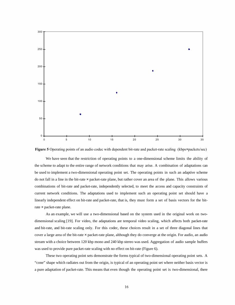
Figure 5 Operating points of an audio codec with dependent bit-rate and packet-rate scaling (kbps×packets/sec)

We have seen that the restriction of operating points to a one-dimensional scheme limits the ability of

the scheme to adapt to the entire range of network conditions that may arise. A combination of adaptations can

be used to implement a two-dimensional operating point set. The operating points in such an adaptive scheme

do not fall in a line in the bit-rate × packet-rate plane, but rather cover an area of the plane. This allows various

combinations of bit-rate and packet-rate, independently selected, to meet the access and capacity constraints of

current network conditions. The adaptations used to implement such an operating point set should have a

linearly independent effect on bit-rate and packet-rate, that is, they must form a set of basis vectors for the bit-

rate × packet-rate plane.

As an example, we will use a two-dimensional based on the system used in the original work on two-

dimensional scaling [19]. For video, the adaptations are temporal video scaling, which affects both packet-rate

and bit-rate, and bit-rate scaling only. For this codec, these choices result in a set of three diagonal lines that

cover a large area of the bit-rate × packet-rate plane, although they do converge at the origin. For audio, an audio

stream with a choice between 120 kbp mono and 240 kbp stereo was used. Aggregation of audio sample buffers

was used to provide pure packet-rate scaling with no effect on bit-rate (Figure 6).

These two operating point sets demonstrate the forms typical of two-dimensional operating point sets. A

“cone” shape which radiates out from the origin, is typical of an operating point set where neither basis vector is

a pure adaptation of packet-rate. This means that even though the operating point set is two-dimensional, there

17

is still a limitation in the independence of bit-rate and packet-rate. This is typical of video codecs, where the

large size of the media unit (the video frame) relative to the network MTU limits aggregation or makes it

impossible. The other typical form an operating point set takes is a grid of points, as in the audio operating

points shown here. This reflects the independence of the bit-rate and packet-rate adaptation made possible by the

use of pure bit-rate and packet-rate adjustments. The small size of an audio sample relative to typical network

MTUs makes these pure adjustments possible, so this form is typical of two-dimensional audio operating point

sets.

0

200

400

600

800

1000

1200

1400

1600

1800

2000

0 10 20 30 40 50 60

Figure 6 Operating points of a codec with two-dimensional video (squares) and audio (circles)

(kbps×packets/sec)

3. Feasible points of an operating point set

As noted above, network conditions may not support some operating points. Other may be undesirable

because of human perceptual constraints. Following Talley [19], we eliminate operating points that are

unsustainable or unsuitable to obtain a set of feasible points, or network box. These feasible points are the only

choices for successful operation in the current network environment.

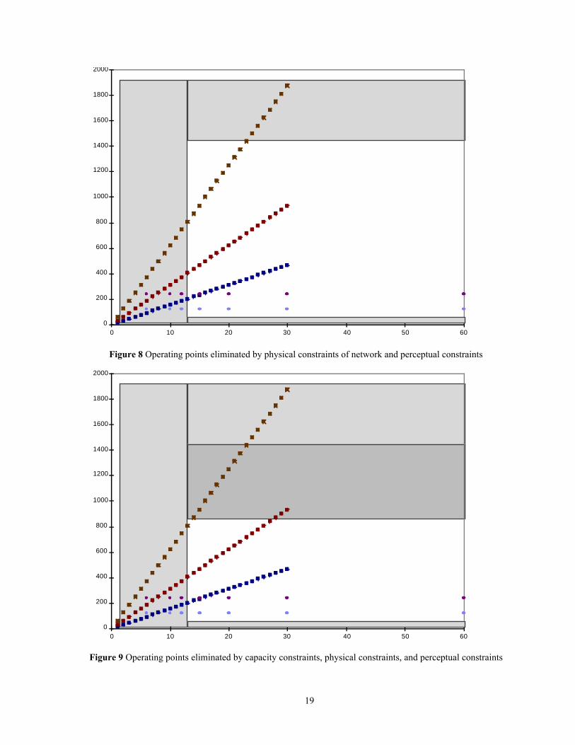
The first unsuitable points we eliminate those points that should be excluded because the quality is too

low for useful conferencing or the latency is too great for useful conferencing (Figure 7). We can also exclude

those points that the codec is physically capable of generating, but which are unsustainable by the network

18

(Figure 8). In this case some of the high frame rate, high quality video is excluded because that is too high a bit-

rate for a slow link (1.544 Mbits/sec) connecting this system to the network. These points are excluded by

fixed limitations of the application and system configuration and should always be excluded from consideration

by the adaptation algorithm.

Now we consider points that are excluded from consideration by network conditions. In a network with

congestion, the right and upper boundaries of the network box are determined by the amount and type of resource

constraints causing the congestion. The bottleneck capacity constraint limits the number of bits that can be

sent. This eliminates the uppermost points of the operating point set (Figure 9). The bottleneck access

constraint likewise limits the number of packets that can be sent. This eliminates the rightmost points of the

operating point set (Figure 10). As the constraints in a given network change over time, the size and shape of

the network box also changes, so dynamic control is needed to make the best use of the network.

0

200

400

600

800

1000

1200

1400

1600

1800

2000

0 10 20 30 40 50 60

Figure 7 Operating points eliminated by perceptual constraints shown in gray shaded over

19

0

200

400

600

800

1000

1200

1400

1600

1800

2000

0 10 20 30 40 50 60

Figure 8 Operating points eliminated by physical constraints of network and perceptual constraints

0

200

400

600

800

1000

1200

1400

1600

1800

2000

0 10 20 30 40 50 60

Figure 9 Operating points eliminated by capacity constraints, physical constraints, and perceptual constraints

20

0

200

400

600

800

1000

1200

1400

1600

1800

2000

0 10 20 30 40 50 60

Figure 10 Operating points eliminated by access constraints, capacity constraints, physical constraints, and

perceptual constraints

4. Heuristics for Adaptation

For a given an operating point set, an adaptation algorithm must select the operating point that is best

suited to the current network conditions. This can be viewed as a twofold optimization.

First, the algorithm must keep operations within the network box. If the current network conditions

contract the network box so that it no longer includes the current operating point, the appropriate adaptation or

adaptations must be applied to move to an operating point within the new network box.

Second, the algorithm should find the best quality operating point in the current network box. In general

points to the upper right of the network box (i.e. points with the maximum feasible bit-rate and packet-rate) are

the best quality operating points because they have the highest fidelity and lowest latency. If a bottleneck

constraint is relieved, the network box expands, and the adaptation algorithm should apply the appropriate

adaptation to take advantage of the higher quality of the newly feasible operating points.

An end-to-end adaptation algorithm relies on feedback from the receiver to provide indications of

congestion. Such indications may include trends in latency, trends in delay-jitter, latency or delay-jitter relative

to a threshold, or packet loss relative to a threshold. From such indications the source can classify the network

as being congested or uncongested. This classification represents the application’s best determination of the

network conditions, and not necessarily the actual state of the network. Since the actual state of the network is

21

both distributed and rapidly changing, a more accurate assessment is impractical. Experience with various forms

of congestion control, most notably TCP [15], has shown that end-to-end detection of congestion can be used

for successful adaptation to network conditions.

The other important aspect of an end-to-end adaptation algorithm is the type of adaptations that the

algorithm can apply. These adaptation types correspond to the two objectives listed above. A retreat adaptation

reduces the bit-rate, packet-rate, or both. It is used in the presence of congestion to move from the current

operating point to an operating point closer to (and hopefully in) the network box. A probe adaptation increases

the bit-rate, packet-rate or both. It is used in the absence of congestion to move closer to the best quality

sustainable operating point (upper right corner of the network box).

Beyond the classification of congested or not congested, it may be possible for detailed feedback to

provide some indication of the degree of congestion and for the adaptive algorithm to interpolate to a feasible

point (e.g., a minor adjustment for a small number of packets lost, and a major retreat for a large number of

packets lost). The appropriateness of this approach depends on the quality and detail of the feedback and on the

operating point set. For example, an operating point set with only five or six operating points is unlikely to

benefit greatly from this level of sophistication.

For a one-dimensional operating point set, a congestion control algorithm is straightforward. Feedback

from the receiver indicates the presence or absence of congestion. Since the operating points lie in a straight

line, there is only one direction to retreat, and one direction to probe. Although the question of degree is still

open, this is a question best considered with the specifics of the operating point set in mind.

In the two-dimensional case, the congestion control algorithm has, by definition, more than a single

available option at any given time. For example, if retreating, a two-dimensional video system may reduce bit-

rate only, through a change in compression parameters, or it may reduce both bit-rate and packet-rate through

temporal video scaling (i.e., frame rate reduction). In general, multiple options can exist for either a retreat or for

a probe. It is necessary, therefore, for the congestion control mechanism to deal with the following concerns: (a)

what action is required by current network conditions, and (b) what adaptation provides the best way of

performing this action. Each of these seemingly simple steps merits further consideration.

One approach to determining the required action, proposed by Talley, is the use of the recent history of

successful adaptations to classify the current network conditions as either access constrained or capacity

constrained. If congestion was most recently relieved by a packet-rate reduction, the network is classified as

access constrained. Otherwise, congestion was last relieved by a bit-rate reduction, and the network is classified

as capacity constrained

As noted above, the type of constraint at the current bottleneck cannot be determined from receiver

feedback because the symptoms are identical. Both constraints cause increased packet delay, increased delay-jitter,

and/or packet loss. Thus, this classification of network conditions cannot be based on a real time measurement

of the network.

22

However, one of the underlying assumptions in an adaptive approach is that network conditions are to

some extent, auto-correlated. That is, current conditions are, with high probability, similar to previous

conditions. This is the underpinning of adaptive approaches which use the current operating point as a start, and

apply adjustments to it. Of course, this property is not perfect; sudden changes in network conditions can occur,

such as a router failure which causes packets to follow a new, more congested route. However, as long as the

adaptive algorithm responds to network conditions quickly enough, the current operating point is a useful

starting point.

The same assumption can be extended to the type of constraint affecting the current network path. The

type of constraint affecting the network path is most probably the same type experienced in the recent past. This

leads to the following two design principles. First, if the network appears congested, the current constraint is

most likely the same as the constraint causing the last period of congestion. Thus, if the network was last

classified as access constrained, and congestion appears again, a reduction in packet-rate is a good first choice for

adaptation. Second, if the network does not appear congested, and we wish to probe for a better operating point,

the best choice is not to probe in a direction that would violate the previous constraint. For example, if the last

constraint was an access constraint, a probe that raises the bit-rate without increasing the packet-rate would be

best.

The recent success heuristic proposed by Talley uses the recent history of the conference to classify the

current network conditions. It can be implemented by a simple finite state machine. The state machine is

summarized in Table 2.

23

The first part of the state name refers to the type of constraint that will be assumed if congestion is

detected. The second part of the name refers to the last action taken. Retreat and wait states are used to assess the

success of the last retreat action. Probe states are used to assess the success of the last probe operation.

We now examine these states in detail:

In the Access Probe state, the last action was a probe to raise the packet-rate. If this introduced no

congestion, then the packet-rate is increased again. A counter can be used to require several feedback messages

indicating no congestion between each increase in packet-rate. If an indication of congestion is received, it is

assumed that the last increase in packet-rate exceeded the current access constraint, and the packet-rate is reduced.

In the Access Wait state, the last action was a successful retreat to lower the bit-rate. Since this indicates

that the network was last capacity constrained, this state serves as a waiting period before beginning to probe for

a higher packet-rate. A counter can be used to require several feedback messages indicating no congestion before

beginning packet-rate probes. If congestion arises during this interval, it is assumed that the previous bit-rate

reduction was not, after all, successful, and a packet-rate reduction is attempted.

In the Access Retreat state, the last action was a retreat to lower the bit-rate. The congestion indication

while in this state is an assessment of the success of the lower bit-rate. If congestion was relieved, it is assumed

the network was capacity constrained, and the next round of probes will increase the packet-rate. If congestion

Table 2 Summary of recent success finite state machine states and transitions

State Congestion Detected No Congestion Detected

Probable

Constraint

Type

Previous

Action

Adaptation New state Adaptation New State

Access Probe Reduce

Packet-rate

Wait

Capacity

Increase

Packet-rate

Probe

Access

Access Wait Reduce

Packet-rate

Retreat

Access

Increase

Packet-rate

Probe

Access

Access Retreat Reduce

Packet-rate

Retreat

Capacity

None Wait

Access

Capacity Probe Reduce

Bit-rate

Wait

Access

Increase

Bit-rate

Probe

Capacity

Capacity Wait Reduce

Bit-rate

Retreat

Capacity

Increase

Bit-rate

Probe

Capacity

Capacity Retreat Reduce

Bit-rate

Retreat

Access

None Wait

Capacity

24

indications persist, the bit-rate reduction is viewed as unsuccessful. The network is now assumed to be capacity

constrained, and a reduction in packet-rate is attempted.

In the Capacity Probe state, the last action was a probe to raise the bit-rate. If this introduced no

congestion, the bit-rate is increased again. A counter can be used to require several samples of no congestion

between each increase in bit-rate. If an indication of congestion is received, it is assumed that the last increase in

bit-rate exceeded the current capacity constraint, and the bit-rate is reduced.

In the Capacity Wait state, the last action was an apparently successful retreat that lowered the packet-

rate. This state serves as a waiting period before beginning to probe for a higher bit-rate. A counter can be used

to require several feedback messages indicating no congestion before beginning bit-rate probes. If congestion is

detected during this interval, it is assumed that the previous packet-rate reduction was not, after all, successful,

and a packet-rate reduction is attempted.

In the Capacity Retreat state, the last action was a retreat to lower the packet-rate. The congestion

indication while in this state is an assessment of the success of the lower packet-rate. If congestion was relieved,

it is assumed the network was access constrained, and the next round of probes will increase the bit-rate. If

congestion is detected during this interval, it is assumed that the previous bit-rate reduction was not, after all,

successful, and a packet-rate reduction is attempted.

Although this heuristic is slightly more complex than the control algorithm for a one-dimensional

scheme, it enables the effective use of a wider variety of operating points than the one-dimensional scheme.

Thus, the greater flexibility of a two-dimensional scheme might enable the two dimensional scheme to sustain

feasible conferences under conditions where a one-dimensional scheme cannot, or, even under conditions where

both schemes are feasible, enable the two-dimensional scheme to deliver better quality streams than a one-

dimensional scheme. If such potential advantages can be demonstrated in practice, the additional complexity of

the two-dimensional scheme is clearly worthwhile. Talley was able to show such benefits in campus-size

internetworks [20]. In the next section, we examine empirical studies extending the approach to lengthy Internet

paths.

III. Internet Experiments with a ProShare Implementation of Media Scaling

A. General remarks on the experiments

The experiments documented here are three different types of experiments to compare the effectiveness of

one-dimensional and two-dimensional media scaling in response to Internet traffic conditions. In this section, we

consider the components used in all experiments. Then each of the three experiments is considered in turn.

1. Implementation of the ProShare Experimental system

ProShare version 1.8 was the base for the videoconferencing system used in these experiments. It was

modified to provide a wider range of operating points, to incorporate several adaptive algorithms, and to

implement continuous monitoring and tracing of videoconferencing data rates and conference quality measures.

The base version of ProShare provides three operating points. The “regular quality” operating point,

which is suitable for both LAN and ISDN operation, supplies 84 kilobit per second, ten frame per second video.

Two “high quality” video operating points each generate 200 kilobits per second video. One of these is the seven

frame per second “sharper” option (about 28.5 per frame), the other is the fifteen frame per second “smoother”

option (about 13.3 kb per frame). These options are set in advance and cannot be changed while the conference is

in progress. A conflict in the video options between two systems conferencing over a LAN is resolved at call

initiation (before any remote video is shown on either side) and is resolved by two rules. First, if the regular

quality option is selected on one system, and the high quality option is selected on the other, both systems use

the regular quality video for this conference. Second, if the high quality option is selected on both systems, but

one system has the smoother option selected and the other has the sharper option selected, both systems use the

smoother option for this conference.

All three options have the same audio operating point. ProShare audio operates at a fixed sixteen kilobit

per second rate. This audio is divided into ten 200 byte “audio frames.” No silence detection is done, so the audio

bit-rate and frame rate is constant in both directions of the conference.

These three video options represent good tradeoffs of resource requirements and conference quality, and,

indeed, were chosen as “sweet spots” where the ProShare video codec made especially effective use of the target

video bit-rate. However, in a congested best-effort environment, such fixed operating points may contribute to

congestion collapse by continuing to offer packets to a network which is already saturated and discarding

packets, and can suffer from excessive packet loss that could seriously impact conference quality, even to the

point of infeasibility.

Despite its orientation toward fixed point operation, ProShare video has an internal interface that allows

on-the-fly changes to video bit-rate and frame rate while a conference was in progress. In fact, the video codec

proved quite robust, and exploitation of this interface in our modified version made it possible to build an

26

adaptive videoconferencing system from ProShare. Frame rates from one frame per second to thirty frames per

second could be supported. However, the number of bits per frame could be adjusted only in a narrow range. In

general, the video bit-rate controller was able to scale video bit-rate and frame-rate in a very nearly linear fashion.

(In fact, variation in motion seemed to affect the bit-rate/frame-rate relationship much more than any nonlinear

component of the scaling).

ProShare video uses interframe encoding. Each video frame encodes changes from key data transmitted in

previous frames. Thus, the video encoding was motion sensitive. In the absence of changes in the image, the

video bit-rate drops to near zero. In the experiments, the human operator provided motion consistent with

conversational behavior, and sufficient to keep the video bit-rate near the target rate of operation. Each frame

contains some key data so that, unlike MPEG, there are no frames without reference data that can be

preferentially discarded. An occasional frame can be lost without noticeable reduction in the quality of the video

playout. However, if too many consecutive frames are lost the video must be stopped and restarted. This process

results in a very noticeable “freeze” in the video. These freezes could be observed in congested conditions during

many of our experiments. A high fraction of video frame loss prevents the video playout from ever successfully

restarting, resulting in a complete lack of video. This level of video loss was observed only in artificial

laboratory conditions with extremely high levels of congestion.

For experiments requiring two-dimensional video scaling, three levels of video compression were

implemented. These were a “large” encoding of 2,800 bytes per frame, a “medium” encoding of 2,100 bytes per

frame, and a “small” encoding with 1,200 bytes per frame. Because of the need to increase the amount of key

data in each frame as the frame rate was reduced, the small frame size could not be maintained below ten frames

per second. Similarly, since less key data was sent with each frame as the frame rate was increased, the codec did

not consistently produce large size frames at frame rates above nineteen frames per second. The levels of

compression did not correspond to discernible qualitative differences in the video image quality, but it is

reasonable to assume that adjustments could be made to the codec to make more effective use of the larger size

encodings and deliver such a qualitative difference.

For experiments systems that required one-dimensional video scaling, the medium size frames were used.

When initiating a conference on a LAN, the initiating ProShare system requests permission from a

permission server. This permission server is configured to restrict the use of LAN bandwidth for

videoconferencing to a level that will not excessively impact the other users of the LAN. Note that the purpose

of this permission server is not to reserve bandwidth for videoconferencing. On the contrary, it exists to

guarantee that a significant portion of LAN bandwidth is reserved for any use except ProShare conferencing. The

LAN may still become congested, but it will not become congested solely due to ProShare traffic. This

permission request feature was unsuitable for our experimental version of ProShare, and was disabled through an

internal interface.

The base version of ProShare used a conservative MTU size of 576 bytes. This size was chosen to

minimize MTU compatibility concerns, since Internet RFC 1122 [2] requires all hosts to accept (and reassemble

27

if fragmented) IP packets of up to this size. However, for our purposes, this was too conservative. Such a small

MTU meant that a video frame could require as many as five packets. The experimental system implemented the

use of the full Ethernet payload size of 1,500 bytes. This was deemed an acceptable design choice because so

many Internet traffic sources or destinations are on the Ethernet. Indeed, no fragmentation of Ethernet MTU size

packets was observed in the experiments.

Even the use of the full Ethernet MTU was quite a reduction from the token ring MTU used in Talley’s

system. In fact, while in Talley’s system, video frames of all three levels of quality fit into one packet, in the

ProShare system only the small frame size fit into one packet.

2. ProShare Reflectors

To allow transmission over lengthy Internet paths while observing the two ProShare endpoints locally,

it was necessary to make use of machines at remote sites as reflectors, that is, machines running background

processes that forward certain types of packets between two other systems. A simple reflector application that

listened on the ProShare UDP port was written for this purpose. It took two system names as parameters and

forwarded all ProShare packets from one system to the other system and vice versa. In addition, it detected the

format of an initial conference set up and modified it to identify itself as the call originator. Thus, a ProShare

call was made from a UNC system to a remote reflector, the remote reflector then returned the modified call set

up to a second UNC system that was the actual call recipient. In this way, the two ProShare systems

communicated with each other through a remote site. Since every packet in either direction traversed the same

path to and from the reflector, the full path for every packet was the same, even if the forward and reverse legs of

the path were different.

In addition, multiple reflector(s) could be chained together so that all the conference packets went through

each reflector machine, allowing almost arbitrary path length. Note that with multiple reflectors, the conference

packets flow through the reflectors in opposite order. For example end system A’s packets flow to reflector R

then to reflector R2 then to end system B, while B’s packets flow through R2 to R1 to A. The system name

parameters for R1 identify A and R2, those for R2 identify R1 and B. Because of the difference in order, there

could be routing differences for the paths taken by packets moving in each direction. Some experiments were

carried out with two reflectors, but all others used one. However, in the two reflector experiments, several

checks of the routes used (by traceroute) showed no difference in the routes taken in each direction.

The machines were identical Intel Pentium 120 MHz processors using identical network adapters,

software, and videoconferencing hardware. The use of remote reflectors allowed the two ProShare machines to be

in close physical proximity. In particular, they shared the same video input, were operated by the same

experimenter and resided on the same Ethernet subnet. Because the machines were on a private, unloaded subnet,

they communicated directly for clock skew measurements. Clock skew was measured to enable measurement of

end-to-end latency of individual media units. These measurements were used for experimental evaluation of the

conferences, not in the actual adaptation algorithms. The skew measurements were made in each direction by

comparing several individual timestamps transmitted from one system to arrival timestamps on the other

28

system. The difference with the minimum absolute value was taken as a measure of clock skew. Although this

method worked well in general, discrepancies were often noted and some runs had measured media unit latencies

that were all offset by tens of milliseconds. Several attempts were made to resolve this problem, and the

technique of measuring clock skew before starting ProShare seemed to minimize the discrepancy. However,

because these skew calculation problems affected many of the earlier runs, the corresponding latency

measurements for these runs must be viewed with some skepticism. This will be noted in the results

descriptions of the appropriate experiments.

B. Experiment Set One (Head to Head Comparisons of One-and Two-Dimensional Scaling)

1. Methodology

Our initial experiments [17] attempted to make use of the bi-directional conferencing capabilities of

ProShare. With bi-directional confenencing, two alternative adaptive algorithms could be run simultaneously

(one on each system in the conference), thus exposing each adaptive method to identical network conditions. It

was hoped that the two schemes could run simultaneously with little or no effect on each other. However, there

were sufficient indications that this was not the case to reduce confidence in the validity of this approach and its

results. Experiment set two, described in Section C, was motivated by the desire to confirm the results of this

set of experiments.

The first set of experiments was conducted using a reflector at a single remote site. The remote site was

the University of Virginia, which at that time passed through twelve hops (twelve machines that processed the

packet in the IP layer, including the routers on the path, and the destination). This gave a round trip length of

twenty-four hops. Experiments consisted of ten minute conferences scattered across five two hour time slots.

The time slots were 10-12:00, 12-14:00, 14-16:00, and 16-18:00.

Reflector

AdaptationScheme 2

Internet

AdaptationScheme 1

Figure 11 Configuration for experiment set one

Our one-dimensional system was based on temporal scaling using only the medium level of

compression. The frame rate was adjusted over a range from six frames per second to thirty frames per second.

Because a medium video frame exceeds the size of an Ethernet MTU, each additional video frame requires two

network packets. To minimize latency, no aggregation is performed. The fixed rate audio requires an additional

29

ten packets and 16,000 bits per second. Audio aggregation was deemed undesirable because at ten audio frames

per second, audio already had an inherent latency of 100 ms, and the additional 100 ms induced by aggregating

two audio frames together would have been too great. Since audio operates at a fixed point, we use the sum of

the video operating point and the fixed audio overhead as the operating points of this system. A plot of these

combined operating points is provided in Figure 12. Note that while the operating points are plotted in the bit-

rate × packet-rate plane, they all lie in a straight line in the plane. This system is consistent with the thinking

behind one-dimensional scaling schemes. Packet-rate is viewed as a secondary concern. The operating point set

is geared toward scaling in the bit-rate dimension via frame rate adjustment, with the packet-rate at a fixed

proportion to the bit-rate. No aggregation is attempted, because that would reduce the packet-rate only, and

increase latency. In a system that views bit-rate as the dominant constraint, there is no incentive to make

reductions in the packet-rate at the cost of latency.

Our one-dimensional system adapted by adjusting the video frame rate. To make the frame rate

adjustments proportional to the current level of operation, the number of frames to increment or decrement by is

one in the range of one to nine fps, two in the range of ten to nineteen fps, three in the range of twenty to

twenty-nine, and a decrement of four at thirty fps. In addition, frame rates below six fps are not used due to

excessive video latency.

Feedback was given by the receiver at one second intervals. This feedback included measurements of

network packet loss and estimated average round trip latency. A loss of more than two packets, or a latency

increase of fifty percent over a moving average of the previous five measurements was taken to indicate

congestion. In this case, the video frame rate was reduced. If feedback indicated no sign of congestion for four

seconds, the frame rate was increased.

A two-dimensional scaling system values both packet-rate and bit-rate adjustments. For this type of

system, an operating point set that covers a large area in the bit-rate/packet-rate plane is desirable. However,

with the video frame size as large or larger than the network MTU, and with no possibility of audio adaptation,

covering a sufficient area of the bit-rate × packet-rate plane is difficult.

Our two-dimensional system used two strategies to increase coverage of the bit-rate × packet-rate plane.

First, all three levels of video compression are used. Second, we use aggregation of audio frames with medium

size video frames to increase the area of the bit-rate × packet-rate plane covered by the combined output of the

audio and video streams. To see how, it is useful to view each medium size frame as a one packet “body” and a

half packet tail (e.g., a medium frame of 2,060 bytes could be packaged as a 1,400 byte body in one packet and a

660 byte tail in the next packet). At frame rates of ten or below, each tail can be aggregated with an audio frame.

Thus, each additional medium size video frame in this range raises the overall packet-rate by one, instead of by

two as would be required without aggregation with one audio frame. In the range of eleven to twenty frames per

second, there are too many video tails to aggregate with the audio frames, so each additional frame requires two

additional packets. Above twenty frames per second, the video frames are frequent enough together that we can

30

aggregate the tail of each additional frame with the currently unaggregated tail of an adjacent frame without

introducing excessive latency (at twenty frames per second or above, the latency introduced by this type of

aggregation is bounded by 50 ms). Thus, in this range, each additional video frame requires only one additional

packet.

The resulting operating points are plotted in the bit-rate × packet-rate plane in Figure 13. The slope

changes in upper line (the medium frame rate) are the result of the changing number of packets per additional

frame as we move from ten and below (one additional packet per additional frame) to the ten to twenty range

(two additional packets per additional frame) to the above twenty range (one additional packet per additional

frame).

Both aggregation of audio with video tails , and video tails with video tails introduce additional latency,

but this rather complex arrangement ensures that the additional latency never exceeds 50 ms. In fact, the

arrangement is implemented with a 50 ms timer for holding small packets that are candidates for aggregation.

Note that the range of bit-rates available varies at each packet-rate. The bit-rate ranges are the largest in

the twenty to forty packet range. This is the range in which this particular system is the most two-dimensional.

(i.e., provides the covers the largest area of the of the bit-rate × packet-rate plane). As we shall see, this is the

range of operation where two-dimensional scaling is the most beneficial for this system.

Our two dimensional system adapted with two types of adjustments. It performed pure bit-rate scaling by

moving between small, medium and large operating points of the same packet-rate. It performed an adjustment

in both packet-rate and bit-rate (but primarily packet-rate) by temporal video scaling (i.e., scaling the video

frame rate). To make the frame rate adjustments proportional to the current level of operation, the number of

frames to increment or decrement by is one in the range of one to nine fps, two in the range of ten to nineteen

fps, three in the range of twenty to twenty-nine, and a decrement of four at thirty fps. In addition, frame rates

below six medium frames per second and three large frames per second are not used due to excessive video

latency.

31

2. Results of experiment set one

This set of experiments had three objectives. The first was to determine how often adaptation was

necessary at all. The second was to compare the difference in feasibility between the two adaptation schemes that

is, could one scheme maintain a usable conference under network conditions where the other could not. The third

was to compare conference quality for those cases where both schemes could maintain a feasible conference.

0

100

200

300

400

500

600

0 10 20 30 40 50 60 70

packets per second

Medium size

Figure 12 Operating points for one-dimensional system, experiments sets one and two

32

0

100

200

300

400

500

600

0 5 10 15 20 25 30 35 40 45 50

2100 Bpf2800 Bpf

1200 Bpf

Figure 13 Two-dimensional operating point set for experiment sets one and two

The first of these goals addressed the issue of whether any adaptation was necessary at all. We judged

adaptation unnecessary if the adaptation schemes rose to the highest quality operating points and stayed there for

more than half the conference. Conditions this favorable were never seen in this round of experiments, so

adaptation was always necessary.

The second goal, comparison of feasibility between the two schemes, failed to showed any difference at

all. This was a major factor in our belief that the interaction between the adaptations of two different schemes

made the head-to-head comparison technique problematic. In other words, it appeared that the aggregate operation

of the two schemes was either feasible or infeasible. The two schemes succeeded or failed based on the ability of

the network to sustain their combined output. Only conditions severe enough not to support the lowest

operating points of both schemes simultaneously would make either scheme fail and, in that case, conditions

were so constrained that both schemes failed to deliver a usable conference.

Nevertheless, since the lowest operating points of the two schemes were quite similar, the frequency with

which both schemes were infeasible is of some interest as a measure of how often any adaptation scheme would

fail to deliver a feasible conference. These results conformed to naive expectations. These results are summarized

in Table 3. During the peak period of the day, conferencing over this path was almost impossible, while early or

late in the day, it was feasible more than half the time. Since the endpoints and reflector for these experiments

33

were academic LANs, the high success rate at 12:00 is consistent with “early in the day” utilization of the

network.

Finally, we wished to compare the quality of the videoconference for the two adaptation algorithms.

Although it was felt that the methodology was too limited to draw definite conclusions, there was some

indication that the two-dimensional scheme delivered higher video throughput.

1D Frame/s Received × Time (in s) 2D Frame/s Received × Time (in s)

1D Audio Latency (in ms) × Time (in s) 2D Audio Latency (in ms) × Time (in s)

1D Network Packets Lost × Time (in s) 2D Network Packets Lost × Time (in s)

Figure 14 Sample experimental results for a conference from experiment set one

34

Table 3 Feasibility results for experiment set one

Time Slot Sustainable Not Sustainable % Sustainable

10:00-12:00 6 3 67%

12:00-14:00 4 4 50%

14:00-16:00 1 11 8%

16:00-18:00 3 9 25%

18:00-20:00 4 5 44%

Overall Percentage 36% 64%

C. Experiment Set Two

1. Methodology

In this set of experiments, the same adaptation was used on both systems. The adaptations were

coordinated through a master/slave arrangement, with the slave mimicing the adaptations selected by the

maseter’s adaptation algorirthm. For comparison purposes, one five minute run of each scheme was run, in

close succession, for each time slot. The order of the two schemes was randomized by a coin toss. Because

network conditions can differ dramatically between the two corresponding runs, it is necessary to examine a large

number of runs to draw meaningful conclusions.

2. Results of Experiment Set Two

The results of experiment set two bore out the observations from experiment set one. For this

implementation, the two-dimensional scheme consistently delivered higher video throughput. This is shown by

the video difference figures, where a positive number shows the two-dimensional scheme delivered more frames

for the corresponding minute. Conversely, a negative number shows the one-dimensional scheme delivered more

frames. Two other measures are presented in the following figures. Audio frame loss rates are presented

separately, to provide both comparison between the schemes and an absolute measure of feasibility. As the

Reflector

AdaptationSlave

Internet

AdaptationMaster

Figure 15 Configuration for Experiment Sets Two and Three

35

figures show, there is no significant difference between the schemes for this measure. The final measure is the

audio latency difference. Here, a positive number represents that the two-dimensional scheme had higher latency.

Indeed, the two-dimensional scheme does have a consistently higher latency than the one-dimensional scheme.

However, the difference is relatively minor, and most of it can be accounted for by the audio aggregation

performed for the small and medium frame sizes, so is an expected trade off.

The results are presented for three reflector configurations. Results for a single reflector at UVa (total of

16 hops) and two reflectors, one at UVa and one at Duke (total of 28 hops), are broken down by time slot.

Results for a single reflector at UW (total of 28 hops) are presented all together, because the number of runs was

much smaller for this configuration.

36

-60

-40

-20

0

20

40

60

80

Figure 16 UVa/Duke/UNC: 10:-12:00 Audio Latency difference (ms)

-60

-40

-20

0

20

40

60

80

Figure 17 UVa/Duke/UNC: 12:-14:00 Audio Latency Difference (ms)

37

-100

-50

0

50

100

150

200

250

300

350

Figure 18 UVa/Duke/UNC: 14-16:00 Audio Latency Difference (ms)

-60

-40

-20

0

20

40

60

80

Figure 19 UVa/Duke/UNC: 16-18:00 Audio Latency Difference (ms)

38

0

1

2

3

4

5

6

7

8

Figure 20 UVa/Duke/UNC: 10-12:00 2D Audio Loss Percentage (%)

0

1

2

3

4

5

6

7

8


39

0

2

4

6

8

10

12

14

16


0

2

4

6

8

10

12


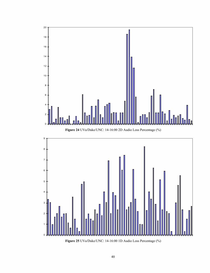
40

0

2

4

6

8

10

12

14

16

18

20


0

1

2

3

4

5

6

7

8

9


41

0

1

2

3

4

5

6

7

8

9


0

5

10

15

20

25

30


42

-15

-10

-5

0

5

10

15

Figure 28 UVa/Duke/UNC: 10-12:00 Video Throughput Difference (fps)

-10

-5

0

5

10

15

20


43

-15

-10

-5

0

5

10

15

20


-15

-10

-5

0

5

10

15

20

25


44

0

5

10

15

20

25

30

35

40

Figure 32 UVa/UNC: 14:00-16:00 Audio Latency Difference (ms)

-20

0

20

40

60

80

100

Figure 33 UVa/UNC: 12-14:00 Audio Latency Difference (ms)

45

-100

-80

-60

-40

-20

0

20

40

60

80


-30

-20

-10

0

10

20

30

40

50

60

70


46

0

1

2

3

4

5

6

Figure 36 UVa/UNC: 10-12:00 2D Audio Loss Percentage (%)

0

1

2

3

4

5

6

7

8


47

0

1

2

3

4

5

6

7

8

9


0

1

2

3

4

5

6

7


48

0

1

2

3

4

5

6

7

8

9


0

5

10

15

20

25


49

0

1

2

3

4

5

6

7


0

1

2

3

4

5

6

7


50

-10

-5

0

5

10

15

20

Figure 44 UVa/UNC: 10-12:00 Video Throughput Difference (fps)

-25

-20

-15

-10

-5

0

5

10

15

20


51

-15

-10

-5

0

5

10

15

20


-10

-5

0

5

10

15

20


52

-80

-60

-40

-20

0

20

40

60

80

100

120

Figure 48 UW/UNC: Audio Latency Difference (ms)

-15

-10

-5

0

5

10

15

20

Figure 49 UW/UNC: Video Throughput Difference (fps)

53

0

5

10

15

20

25

30

35

Figure 50 UW/UNC: 2D Audio Loss Percentage (%)

0

5

10

15

20

25

30

35

Figure 51 UW/UNC: 1D Audio Loss Percentage (%)

54

D. Experiment Set Three

1. Methodology

Because experiment set one had failed to show a feasibility advantage for the two-dimensional ProShare

system, we decided to build a system specifically designed to maximize feasibility vs. a comparable one-

dimensional system. Since the quality of the audio stream is the primary determinant of conference feasibility,

and since the previous system had only a single audio operating point, incorporation of a richer audio

component was a natural next step. Unfortunately, the results, presented in the next section, did not live up to

expectations [18]. However, as an illustration of an experimental two-dimensional audio scaling system, and as

a possible first step toward a more successful implementation, this system is worthy of some discussion.

The modified form of ProShare discussed above was the framework for this implementation as well,

providing a video component, call set up, and UDP based transport. However, the previous two-dimensional

video operating points relied on aggregation with audio to achieve much of its coverage of the bit-rate × packet-

rate plane. Since most of the new audio “frames” were too large for aggregation, the coverage provided by video

alone was greatly reduced. Also, the audio component was the focus of this implementation so it was decided to

use only a simple one-dimensional video component for both the one- and two-dimensional schemes. The frame

size was kept at the “medium” setting of 2,100 bytes per frame. The minimum frame rate was kept at six frames

per second, but the highest frame rate permitted was fourteen frames per second. This restriction was necessary

because the demands on the system (e.g. over twenty additional interrupts per second) of the audio card at its

highest quality operating points interfered with the operation of video at more that fourteen frames per second.

To implement a two dimensional audio system, we planned to vary two attributes of the audio stream

produced by a simple PCM audio codec. First the bit-rate would be varied by changing the sample rate of the

card. Although use of a combination of compression schemes as described in Table 1 would deliver better human

perceived quality at the lower bit-rates, the sample rate approach was sufficient for our purposes. The audio

packet-rate was varied by changing the buffer size given to the card. For example, giving the card 256 byte

buffers to fill with samples and sending each buffer in its own packet, results in a packet-rate twice that of

giving the card 512 byte buffers. The audio sample buffer size is limited by network MTU size, since there is no

point in buffering more samples than can be shipped in on network packet, but this is important only for higher

sample rate. For example, 22,000 one byte samples cannot be squeezed into less than fifteen Ethernet packets,

while 11,000 one byte samples fit comfortably in eight Ethernet packets. For low sample rates, the primary

limit on buffer size is the latency introduced by buffers. For example, aggregating 1,500 one byte samples from

a card sampling at 5,500 samples per second, while possible on an Ethernet, is undesirable because the latency

of 273 ms introduced is too high for conferencing applications.

The two-dimensional operating point set developed after these considerations were taken into account is

shown in Figure 52. As is typical, the one-dimensional operating point set was a subset of the two-dimensional

55

set. The one-dimensional scheme we wished to compare to was bit-rate scaling, so any of the three columns of

audio operating points would have been a suitable choice. We chose to use the rightmost column for two

reasons: it had the most points in a single column, and it introduced the lowest packaging latency of the three

columns.

The original ProShare audio component was still part of the implementation, but its effect on the bit-rate

and packet-rate of this implementation was reduced to a trivial level. First, the ProShare audio mute function

was used to eliminate the flow of audio data. Unfortunately, the audio component continued to transmit ten

empty audio “frames” a second. Lacking total access to ProShare internals, I could not find a satisfactory way to

turn off this flow of packets. Initial experiments with this implementation continued to transmit these empty

frames each in their own packet. About half way through, a packaging enhancement was added to at least

package these empty frames with other data. The enhancement was designed to favor packaging with video, but

this was not strictly managed. Thus, the last effect of the existing ProShare audio component was all but

eliminated. However, there is no significant change in the results corresponding to the deployment of the

packaging enhancement, so we can conclude that the fixed ten packet per second flow of empty ProShare audio

packets did not favor one adaptation scheme over the other, and consider the results before and after the

enhancement as a whole. Two hardware issues prevented a straightforward implementation of the desired

operating point set. Instead a simulation was done. This simulation still used the sound card, and still produced

the bit-rate packet-rate combinations shown in Figure 52. The first problem with the implementation of a

variable sample rate was that the available sound card could not run at different sample rates for input and

output. This meant that even if the adaptations of the two systems participating in the conference were

coordinated, there would still be transitional periods where the audio from the remote system could not be played

because the sample rate did not match the rate in use on the local system. Thus, the decision was made to not

play the audio at the receiver. The audio was still transmitted, which was sufficient for the research goals of this

system. Although playable audio is a useful check on the quality of transmission, actually judging the

feasibility can be done with empirical quality measures of audio loss and latency, so actual playout of the

transmitted audio was not essential. Once playable audio was no longer a goal, further simulation to circumvent

a second problem seemed entirely appropriate.

56

The second problem was that changing the sampling rate required closing and reopening the card.

Although for previous work with the sound card on other projects this was a minor concern, when incorporated

into the ProShare framework the close and reopen process introduced a noticeable drop in bit-rate and packet-rate.

Because each adaptation implied a potential close and reopening of the card, this was a serious concern.

Therefore, it was decided to simulate changing sample rates, but operate the card at a single rate, thus avoiding

the close and reopen overhead.

To simulate the operating points in Figure 52, two notions of buffer size were introduced. First, a record

buffer size was used to generate the sound card interrupt rate (and thus the proper packet-rate). Since the card

operated at 5,500 samples per second, to simulate a rate of 22,000 samples per second and 1,024 byte buffers,

the record buffer size was 256 (i.e.,

22 00

1 024

5 500

256215

, /

,

,.

samples second

samples/ interrupt

samples / second

samples / interruptinterrupts/ second= ≈ ).

Of course, to simulate the bit-rate of the 22 kHz, 1,024 byte buffer operating point, it is necessary to

transmit 1,024 bytes per interrupt, not just the 256 bytes filled by the sound card. So, each simulated operating

point also had a defined transmit buffer size, the number of bytes that would have been both filled by the sound

card and transmitted on the network for the simulated operating point.

0

50

100

150

200

250

0 5 10 15 20 25 30

Packet Rate

Bit Rate (kbps)

5 kHz8 kHz11kHz

16kHz22 kHzVideo

Figure 52 Experiment Set Three Operating Point Set

57

The record buffer sizes and transmit buffer sizes used to simulate all the operating points are listed in

Table 4.

2. Results of Experiment Set Three

The experiments were conducted using two reflector configurations, the UVa/Duke/UNC configuration

(28 hops), and the UW/UNC configuration (28 hops). As before, five minute runs were done during the 10:00-

18:00 time period, with at least a ninety minute gap between runs for the same configuration. The runs were

conducted in late June and early July of 1997.

As noted above, the results do not show a significant advantage for either scheme, using either

configuration. First, we will compare the performance of the schemes by four criteria. Then we will conclude

this section with a discussion of the results and possible future work based on the two-dimensional audio

implementation.

The first point of comparison is audio throughput, measured by the difference in delivered audio bit-rate.

It was expected that the two-dimensional scheme would deliver a higher bit-rate, because under an access

constraint, the two-dimensional scheme could reduce audio packet-rate without reducing audio bit-rate, while the

one-dimensional scheme would vainly reduce audio bit-rate in response to the symptoms of congestion.

However, the one-dimensional scheme delivered a higher bit-rate in 60 out of 110 minutes of videoconferencing

in the UVa/Duke/UNC configuration (Figure 53) and 54 out of 100 minutes of videoconferencing in the

UW/UNC configuration (Figure 54). So, the one-dimensional scheme appeared to do slightly better by this

measure.

Table 4 Simulation Values for Audio Operating Points

Simulated Sample Rate (kHz) Record Buffer Size (bytes) Transmit Buffer Size (bytes)

22 256 1024

16.5 256 768

16.5 384 1152

11 256 512

11 384 768

11 512 1024

8.25 256 384

8.25 384 536

8.25 512 768

5.5 256 256

5.5 384 384

5.5 512 512

58

The second point of comparison is video throughput, measured by the difference in delivered video frame

rate. In this case, the two-dimensional scheme delivers more video in 62 out 110 minutes for the

UVa/Duke/UNC configuration (Figure 55) and 49 out of 100 minutes for the UW/UNC configuration (Figure

56).

The third point of is the ability to deliver feasible conferences. We make this comparison by defining and

absolute measure of feasibility, and measuring how many minutes of conferencing each scheme succeeds or

fails. Our measure of feasibility is chosen as a 3% loss rate for all transmitted packets. For the UVa/Duke/UNC

configuration, the two-dimensional scheme (Figure 57) had only 10 infeasible minutes, and the one-dimensional

scheme (Figure 58) had 11. For the UW/UNC configuration, the two-dimensional scheme (Figure 59) had 28

infeasible minutes and the one-dimensional scheme had 27. Twenty-one of these occurrences of infeasibility

were mutual, in that both schemes were infeasible in their respective minutes of conferencing. Indeed, heavy

clustering of high loss rates in both figures indicates a few days of heavy congestion were responsible for most

of the infeasible minutes for both schemes in this configuration. (In contrast, there were no instances in the

UVa/Duke/UNC configuration where both schemes were infeasible for the same corresponding minutes.) We

conclude that neither scheme had a significant advantage by this criterion.

The final point of comparison is latency, measured here by video latency. Again, there was no significant

difference here. The two-dimensional had higher latency in 62 of the 110 minutes in the UVa/Duke/UNC

configuration (Figure 61), but all of the latency differences were below the 71 ms interframe gap of even the 14

frame per second operating point. The one-dimensional scheme did have 6 latencies worse by more than 71 ms.

The two-dimensional scheme had a higher latency in the UW/UNC configuration 62 out of 100 minutes, with

10 minutes above the 71 second level. However, 5 of these were during mutually infeasible minutes, when

network conditions were extremely bad. We conclude that there is perhaps a slight advantage to the one-

dimensional scheme for the latency measure.

These results were disappointing, because the areas this implementation was intended to improve, audio

quality and conference feasibility, were the same or slightly worse than the one-dimensional system, while video

throughput like the previous implementations, was the clear advantage for the two-dimensional scheme. It is

possible, however, to identify two areas for improvement in this implementation that might yield more

favorable results.

First, the video component of both systems was identical. If a video component that was two-

dimensional (on its own) could be combined with the two-dimensional audio component, this might provide

more differentiation in adaptation that between the two schemes in this implementation. Second, it is possible

that refinements of the adaptation control algorithm could improve the performance of the two-dimensional

scheme. One possibility would be changes to the timing values, which were unchanged from the previous

implementations. Another possibility would be to perform separate the network classification and quality

measurement for the audio and video streams, allowing different adaptations (and perhaps even different control

algorithms) for each stream.

59

-100

-80

-60

-40

-20

0

20

40

60

80

100

Figure 54 UW/UNC: Audio bit-rate difference (kbps)

-100

-80

-60

-40

-20

0

20

40

60

80

100

Figure 53 UVa/Duke/UNC: Audio Bit-rate Difference (kbps)

60

-8

-6

-4

-2

0

2

4

6

8

Figure 55 UVa/Duke/UNC: Video Frame Rate Difference (fps)

-8

-6

-4

-2

0

2

4

6

8

Figure 56 UW/UNC: Video Frame Rate Difference (fps)

61

0

2

4

6

8

10

12

14

16

Figure 57 UVa/Duke/UNC: Two-Dimensional Scheme Packet Loss Percentage (%)

0

2

4

6

8

10

12

14

16

Figure 58 UVa/Duke/UNC: One-Dimensional Scheme Packet Loss Percentage (%)

62

0

2

4

6

8

10

12

14

16

Figure 59 UW/UNC: Two-Dimensional Scheme Packet Loss Percentage (%)

0

2

4

6

8

10

12

14

16

Figure 60 UW/UNC One-Dimensional Scheme Packet Loss Percentage (%)

63

-100

-80

-60

-40

-20

0

20

40

60

80

100

Figure 61 UVa/Duke/UNC: Latency Difference (ms)

-100

-75

-50

-25

0

25

50

75

100

Figure 62 UW/UNC Latency difference (ms)

IV. Conclusions

A. Summary

Taken as a whole, our experiments are a positive outcome in favor of two-dimensional scaling. First, it

was possible to implement a two-dimensional scaling system for ProShare, which was not in fact designed with

media scaling in mind at all. Second, although the ProShare implementation did not provide as wide a coverage

of the bit-rate × packet-rate plane as the earlier experimental system, it delivered a consistent, measurable benefit

in the form of a higher video frame rate. Detailed examination of the experimental data indicates that this benefit

is most noticeable when the system is operating in the twenty to forty packet per second range, where the

operating point set provides the widest coverage of the bit-rate × packet-rate plane. This supports the conclusion

that it is the availability of these additional adaptations that makes this benefit possible. Finally, it is worth

noting that even over paths of nearly twice the length of typical Internet paths, the system enjoyed a reasonable

rate of success in delivering feasible videoconferences.

Although the results of experiment set three which implemented the two-dimensional audio component,

were more disappointing, there are some additional factors worth further consideration. First, since this system

was tested on lengthy paths, it is possible that it reached a scale where the effectiveness of two-dimensional

adaptation is too limited to be noticeable. Since two-dimensional adaptation is effective at smaller scales, and

since the two-dimensional scheme in experiment set three did not perform significantly worse than the one-

dimensional scheme, the two-dimensional method is still valuable for general purpose use. Second, it is quite

possible that a refinement of this system could yield a more positive result. Two possible enhancements are fine

tuning the parameters of the recent success implementation, and adding a two-dimensional video component.

B. Issues for further research

There are additional issues raised by this work that are potential topics of further research. First, in the

issue of codec design, there are the challenges of designing a codec that provides a rich, robust set of operating

points. Since many codecs are not even capable of one-dimensional scaling, improved flexibility would appear

to be a worthwhile goal. A second issue is introduced by an informal observation made while conducting the

experiments. Occasionally, the frame rate observed by the experimenter appeared to be less than the monitoring

tool was measuring as delivered. This means that frames were making it through the network, but were not

displayed by the video manager. We can assume that they arrived too late to be played out successfully, and

therefore fall into the category of data that is transmitted but not used, one of the contributors to congestion

collapse. Of course, the key data in such frames may still have been of some use. Nevertheless, we conclude that

it would be useful for a codec to communicate to the adaptation control mechanism that although a frame arrived

successfully, it was unplayable. Such an event could serve as an indication of congestion that would contribute

65

to the accuracy of congestion detection based on packet statistics alone. In these two areas, and perhaps others,

codec design could be directed toward the goal of control by an adaptive algorithm.

Another issue raised in conjunction with this work is the reaction to a recent proposal for router based

enforcement of conformance to TCP congestion control [11]. This proposal was motivated by the growing

number of multimedia applications that indulge in behavior such as sending at a constant bit-rate that can have a

negative impact on other users of the network, in particular TCP. The effect on TCP applications is of

particular interest because TCP is widely used and has been shown to be very effective in preventing congestion

collapse. However, enforcing strict conformance to TCP congestion control may be unnecessarily restrictive.

For example, two-dimensional scaling as implemented here operates at a different time scale from TCP, and

would probably not be conformant to TCP congestion control. However, it does adapt in response to symptoms

of congestion, and does so in ways that are appropriate to the videoconferencing domain. In fact, by making use

of more detailed feedback than TCP, which depends on packet loss, it may detect and adapt to congestion more

quickly in some cases. However, it is a meaningful requirement that adaptive schemes be effective in preventing

congestion collapse. This remains to be demonstrated for two-dimensional scaling and other proposed adaptive

methods, so obtaining measurements relevant to this question is, therefore, an interesting area of future research.

A second justification for the proposal to enforce TCP conformance is the question of fairness to TCP.

This is, however, much less compelling. It is impossible for an end-to-end adaptation scheme to measure its

effect on other applications and avoid impacting them in a negative way, (e.g., avoid stealing bandwidth). In

fact, TCP applications can be, and are, unfair to each other to a certain extent. Thus, issues of fairness should be

dealt with in more flexible ways, such as providing a service classes with scheduling policies such as weighted

fair queueing to prevent different adaptive algorithms from negatively impacting each other. However, since it

will be some time before service classes could be available, the question of whether a typical two-dimensional

scaling scheme such as the one discussed is in fact, consistently unfair to TCP is of some interest.

To summarize, this work has reaffirmed the utility of two-dimensional media scaling as an approach to

videoconferencing on best-effort networks in general and the Internet in particular. Further exploration of this

approach, including an examination of its interaction with other Internet applications is a promising area for

further research.

V. References

[1] Bolot, J., Turletti, T., A Rate Control Mechanism for Packet Video in the Internet, Proc. IEEEINFOCOMM Ô94, Toronto, Canada, June 1994, pp. 1216-1223.

[2] Braden, R. (Ed.), Requirements for Internet Hosts Ð Communication Layers. Network Working Group,RFC 1122, October 1989.

[3] Braden, R., D. Clark, and S. Shenker, Integrated Services in the Internet Architecture: an Overview,IETF RFC-1633, July 1994.

[4] Chakrabarti, S., Wang, R., Adaptive Control for Packet Video, Proc. IEEE International Conference onMultimedia Computing and Systems 1994, Boston, MA, May 1994, pp. 56-62.

[5] Cruz, R., A calculus for network delay, part I: Network elements in isolation, IEEE Transaction onInformation Theory, 37(1):114-121, 1991.

[6] Delgrossi, L., Halstrick, C., Hehmann, D., Herrtwich, R., Krone, O., Sandvoss, J., Vogt, C., MediaScaling for Audiovisual Communication with the Heidelberg Transport System, Proc. ACMMultimedia Ô93, Anaheim, CA, Aug 1993, pp. 99-104.

[7] Dempsey, B., and Zhang, Y., Destination Buffering for Low-Bandwidth Audio Transmissions UsingRedundancy-Based Error Control, 21st IEEE Local Computer Networks Conference, Minneapolis, MN,October 1996, pp. 345 Ð 355.

[8] Ferrari, D. Client Requirements for Real-Time Communication Services, IEEE CommunicationsMagazine, pp. 65-72, November, 1990.

[9] Ferrari, D., Banjea, A., and Zhang, H., Network Support for Multimedia: A Discussion of the TenetApproach, Computer Networks and ISDN Systems, Vol. 26, No. 10 (July 1994), pp. 1267-1280.

[10] Floyd, S., Jacobson, V., Random Early Detection Gateways for Congestion Avoidance, IEEE/ACMTransactions on Networking, 1(4):397-413, Aug. 1993.

[11] Floyd, S., Fall, K., Router Mechanisms to support End-to-End Congestion Control, Technical Report,1997. URL ftp://ftp.ee.lbl.gov/papers/collapse.ps

[12] Hardman, V., Sasse, M., Handley, M., and Watson, A. Reliable Audio for Use over the Internet, Proc.of INET '95, pp. 27-30, Honolulu, Hawaii, USA, June 1995.

[13] Hoffman, Don, Spear, M., Fernando, Gerard, Network Support for Dynamically Scaled MultimediaStreams, Network and Operating System Support for Digital Audio and Video, Proceedings, D.Shepard, et al (Ed.), Lecture Notes in Computer Science, Vol. 846, Springer-Verlag, Lancaster, UK,November 1993, pp. 240-251.

67

[14] Huitema, C., Routing in the Internet, Prentice Hall PTR, Englewood Cliffs, NJ, 1995.

[15] Jacobson, V., Congestion Avoidance and Control, Proc. ACM SIGCOMM Õ88 Conf., ACM, pp.314-329, August, 1988.

[16] Jeffay, K., Stone, D.L., Smith, F.D., Kernel Support for Live Digital Audio and Video, Proc, 2nd Intl.Workshop on Network and Operating System Support for Digital Audio and Video, Heidelberg,Germany, Lecture Notes in Computer Science, Springer-Verlag, Vol. 614, pp. 10-21, Springer Verlag,Heidelberg, 1992.

[17] Nee, P., Jeffay, K., Danneels, G., The Performance of Two-Dimensional Media Scaling for InternetVideoconferencing, Proc. 7th Intl. Workshop on Network and Operating System Support for DigitalAudio and Video, St. Louis, MO, May 1997.

[18] Nee, P., Jeffay, K., Clark, M., Danneels, G., A Two-Dimensional Audio Scaling Enhancement to anInternet Videoconferencing System, Proc. Intl. Workshop on Audio-Visual Services over PacketNetworks, to appear.

[19] Talley, T.M., Jeffay, K., Two-Dimensional Scaling Techniques for Adaptive, Rate Based TransmissionControl of Live Audio and Video Streams, Proc. Second ACM Intl. Conference on Multimedia, SanFrancisco, CA, October 1994, pp. 247-254.

[20] Talley, T.M., Jeffay, K., A General Framework for Continuous Media Transmission Control,Proceedings of the 21st IEEE Conference on Local Computer Networks, Minneapolis, MN, October1996, pages 374-383.

[21] Topolcic, C. (Ed.), Experimental Internet Stream Protocol, Version 2 (ST-II). Network WorkingGroup, RFC 1190, IEN-119, CIP Working Group, October 1990.

[22] Wolf, C., Video Conferencing: Delay and Transmission Considerations, in Teleconferencing andElectronic Communications: Applications, Technologies, and Human Factors, L. Parker and C. Olgren(Eds.), 1982.

[23] Zhang, L., Deering, S., Estrin, D., Shenker, S., Zappala, D., RSVP: A New Resource ReSerVationProtocol, IEEE Network, Vol. 5, No. 5 (September 1993), pp. 8-18.

Experimental Evaluation of Two-Dimensional Media Scaling

Documents

Transcript of Experimental Evaluation of Two-Dimensional Media Scaling