Experimental Design For Injection Molding 1 Launsby Consulting Experimental Design For Injection...
153
Launsby Consulting 1 4/2/2009 Experimental Design For Injection Molding Launsby Consulting 2009
Transcript of Experimental Design For Injection Molding 1 Launsby Consulting Experimental Design For Injection...
Launsby Consulting14/2/2009
Experimental Design For Injection Molding
Experimental Design For Injection Molding
Launsby Consulting2009
Launsby Consulting2009

Launsby Consulting4/2/2009 2
Bob LaunsbyBob Launsby
• Taught experimental design to several thousand people
• Participated in numerous actual experiments
• Application is key• Co-developer of DOE Wisdom software• Co-Author of “DOE for Injection Molding”
• Taught experimental design to several thousand people
• Participated in numerous actual experiments
• Application is key• Co-developer of DOE Wisdom software• Co-Author of “DOE for Injection Molding”
www.launsby.com

Launsby Consulting4/2/2009 3
IntroductionsIntroductions
• Name• Title• Background in Injection Molding
– Previous Courses– Cavity Pressure Control?
• Previous Experiences with Experimental Design and Statistics
• Name• Title• Background in Injection Molding
– Previous Courses– Cavity Pressure Control?
• Previous Experiences with Experimental Design and Statistics
Launsby Consulting4/2/2009 4
Course GuidelinesCourse Guidelines
• Start and Stop Times• Breaks• Active Participation• You are Responsible for Learning• Importance of Applications
• Having Fun and Learning
• Start and Stop Times• Breaks• Active Participation• You are Responsible for Learning• Importance of Applications
• Having Fun and Learning

Launsby Consulting4/2/2009 5
Module OneModule One
• Goals:– Understand the Building Blocks for a
Fundamentally Robust Molding Process– Understand the Need for Modern Design of
Experiments Techniques– Recognize the Power and Applicability of
These Approaches to Injection Molding– Understand the Basics
• Goals:– Understand the Building Blocks for a
Fundamentally Robust Molding Process– Understand the Need for Modern Design of
Experiments Techniques– Recognize the Power and Applicability of
These Approaches to Injection Molding– Understand the Basics
Launsby Consulting4/2/2009 6
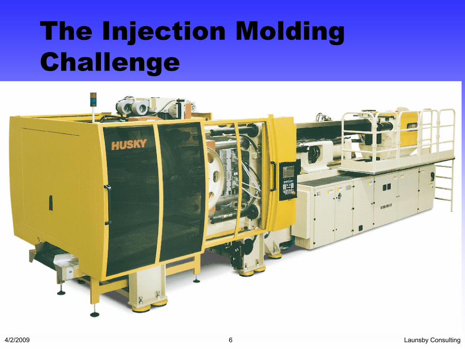
The Injection MoldingChallenge

Launsby Consulting4/2/2009 7
The Challenge(Cont.)The Challenge(Cont.)• Complex Part Geometry,Many Finishes• Varying Wall Thickness• Snap Fits, Threads• No Secondary Operations• Consistency, High Prod. Rates• Regrind • Tight Tolerances, Cost Competition• QS 9000, Process Validation
• Complex Part Geometry,Many Finishes• Varying Wall Thickness• Snap Fits, Threads• No Secondary Operations• Consistency, High Prod. Rates• Regrind • Tight Tolerances, Cost Competition• QS 9000, Process Validation

Launsby Consulting4/2/2009 8
The Process DiagramThe Process Diagram

Launsby Consulting4/2/2009 9
PROCESS DIAGRAM FOR
INJECTION MOLDING
Some Potential FactorsMaterial Lot
Material Variation
% Regrind
Hold Pressure
Pellet Geometry
Plastic Temperature
Screw RPM
Injection Velocity
Potential ResponsesDimensions
Color
Black Specks
Warpage
Blisters
Blush
Knit Lines
Sinks
Process DiagramProcess Diagram

Launsby Consulting4/2/2009 10
Basic Understandings Before DoeBasic Understandings Before Doe• Non-Newtonian Behavior of Plastic
– Static Pressure Loss– Relative Viscosity Curves
• Semi-Crystalline Vs. Amorphous Materials• Hygroscopic and non-hygroscopic
Materials• Shear Heating• Fountain Flow• Four Plastic Variables
• Non-Newtonian Behavior of Plastic– Static Pressure Loss– Relative Viscosity Curves
• Semi-Crystalline Vs. Amorphous Materials• Hygroscopic and non-hygroscopic
Materials• Shear Heating• Fountain Flow• Four Plastic Variables
Launsby Consulting4/2/2009 11
Static Pressure LossStatic Pressure Loss
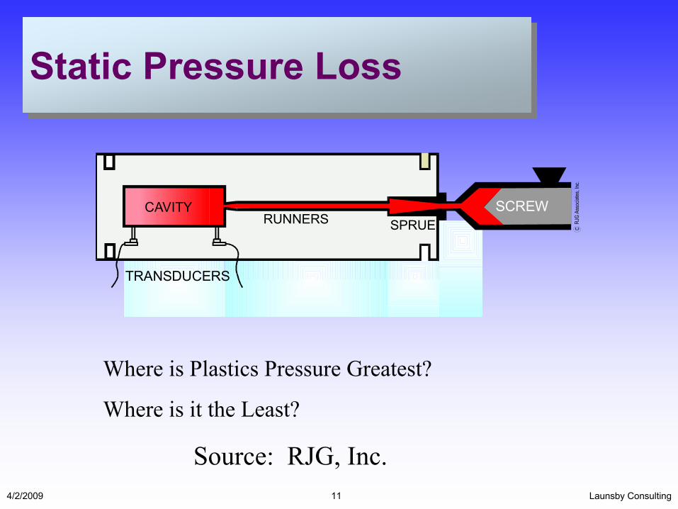
TRANSDUCERS
SPRUERUNNERSSCREWCAVITY
Where is Plastics Pressure Greatest?
Where is it the Least?
Source: RJG, Inc.
Launsby Consulting4/2/2009 12
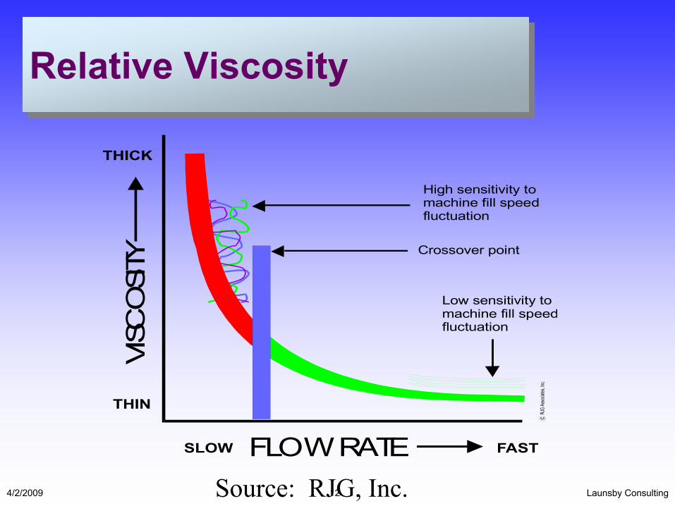
Relative ViscosityRelative Viscosity
VISC
OSI
TYTHICK
THIN
SLOW FASTFLOWRATE
High sensitivity tomachine fill speedfluctuation
Crossover point
Low sensitivity tomachine fill speedfluctuation
Source: RJG, Inc.
Launsby Consulting4/2/2009 13
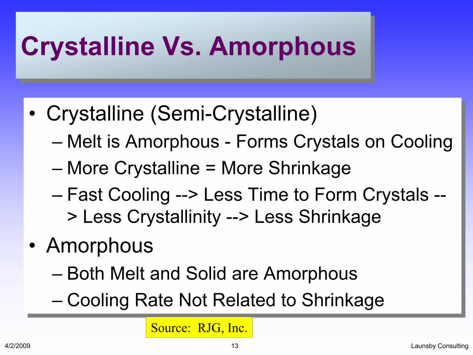
Crystalline Vs. AmorphousCrystalline Vs. Amorphous
• Crystalline (Semi-Crystalline)– Melt is Amorphous - Forms Crystals on Cooling– More Crystalline = More Shrinkage– Fast Cooling --> Less Time to Form Crystals --
> Less Crystallinity --> Less Shrinkage• Amorphous
– Both Melt and Solid are Amorphous– Cooling Rate Not Related to Shrinkage
• Crystalline (Semi-Crystalline)– Melt is Amorphous - Forms Crystals on Cooling– More Crystalline = More Shrinkage– Fast Cooling --> Less Time to Form Crystals --
> Less Crystallinity --> Less Shrinkage• Amorphous
– Both Melt and Solid are Amorphous– Cooling Rate Not Related to Shrinkage
Source: RJG, Inc.

Launsby Consulting4/2/2009 14
Fountain FlowFountain Flow
• Fountain Flow, Skin Layer, and Alignment• Fountain Flow, Skin Layer, and Alignment
Source: RJG, Inc.

Launsby Consulting4/2/2009 15
Four Plastic VariablesFour Plastic Variables
• Plastic Flow Rate• Plastic Temperature• Plastic Cooling• Plastic Pressure Gradient
• Plastic Flow Rate• Plastic Temperature• Plastic Cooling• Plastic Pressure Gradient
Launsby Consulting4/2/2009 16
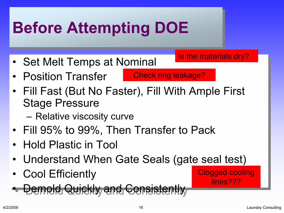
Before Attempting DOEBefore Attempting DOE
• Set Melt Temps at Nominal• Position Transfer• Fill Fast (But No Faster), Fill With Ample First
Stage Pressure– Relative viscosity curve
• Fill 95% to 99%, Then Transfer to Pack• Hold Plastic in Tool• Understand When Gate Seals (gate seal test)• Cool Efficiently• Demold Quickly and Consistently
• Set Melt Temps at Nominal• Position Transfer• Fill Fast (But No Faster), Fill With Ample First
Stage Pressure– Relative viscosity curve
• Fill 95% to 99%, Then Transfer to Pack• Hold Plastic in Tool• Understand When Gate Seals (gate seal test)• Cool Efficiently• Demold Quickly and Consistently
Check ring leakage?
Clogged cooling lines???
Is the materials dry?

Launsby Consulting4/2/2009 17
What Is A Designed Experiment?What Is A Designed Experiment?• Systematic, Controlled Changes of the
Inputs (factors) to a Process in Order to Observe Corresponding Changes in the Outputs (responses).
• Systematic, Controlled Changes of the Inputs (factors) to a Process in Order to Observe Corresponding Changes in the Outputs (responses).
Launsby Consulting4/2/2009 18
Types Of FactorsTypes Of Factors
• Constant Factors• Control Factors • Noise Factors (Robustness)
• Constant Factors• Control Factors • Noise Factors (Robustness)
Launsby Consulting4/2/2009 19
What Do We Learn From Designed Experiments?What Do We Learn From Designed Experiments?
• Best Settings
• Sensitivity
• Best Settings
• Sensitivity
Launsby Consulting4/2/2009 20
Why Do Designed Experiments?Why Do Designed Experiments?
• 50 Per Cent Improvement in Efficiency and Effectiveness
• 1 + 1 = 10
• 50 Per Cent Improvement in Efficiency and Effectiveness
• 1 + 1 = 10

Launsby Consulting4/2/2009 21
How To Be Good At ItHow To Be Good At It
• Attend Training
• Read
• 510 Rule
• Attend Training
• Read
• 510 Rule
Launsby Consulting4/2/2009 22
Engineering Experimental DesignEngineering Experimental Design• Not a Substitute For Knowledge of
Technology• Incorporates Current Understanding
• Physics First• If You Do Not Understand the Basics, You
Will Do EVIL Things With DOE
• Not a Substitute For Knowledge of Technology
• Incorporates Current Understanding
• Physics First• If You Do Not Understand the Basics, You
Will Do EVIL Things With DOE
Launsby Consulting4/2/2009 23
Examples Of Poorly Done Doe’s Examples Of Poorly Done Doe’s • Quality Digest of 1999
– Injection Press– Gates– Barrel Temps– Moisture Content– Randomization, Replication
• Quality Digest of 1999– Injection Press– Gates– Barrel Temps– Moisture Content– Randomization, Replication
Launsby Consulting4/2/2009 24
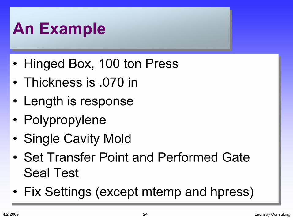
An ExampleAn Example
• Hinged Box, 100 ton Press• Thickness is .070 in• Length is response• Polypropylene• Single Cavity Mold• Set Transfer Point and Performed Gate
Seal Test• Fix Settings (except mtemp and hpress)
• Hinged Box, 100 ton Press• Thickness is .070 in• Length is response• Polypropylene• Single Cavity Mold• Set Transfer Point and Performed Gate
Seal Test• Fix Settings (except mtemp and hpress)

Launsby Consulting4/2/2009 25
An ExampleAn Example
RUN Mtemp H Press Length
1 70 5000 15
2 70 7000 19
3 90 5000 12
4 90 7000 17
Launsby Consulting4/2/2009 26
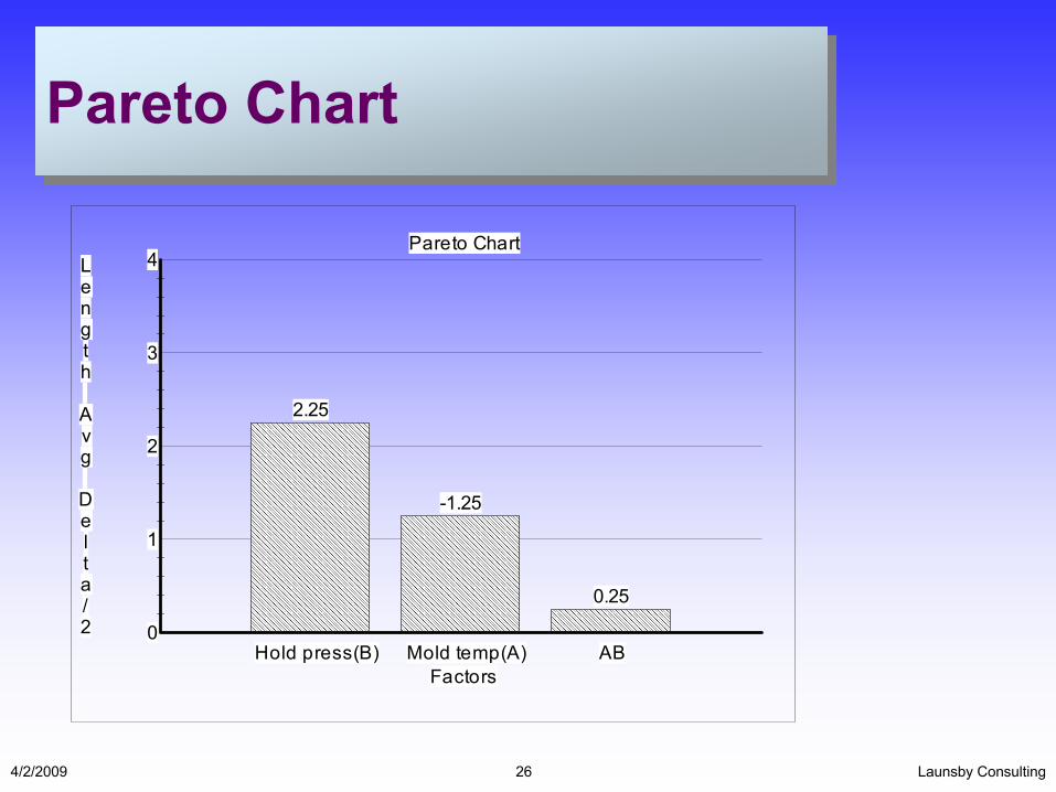
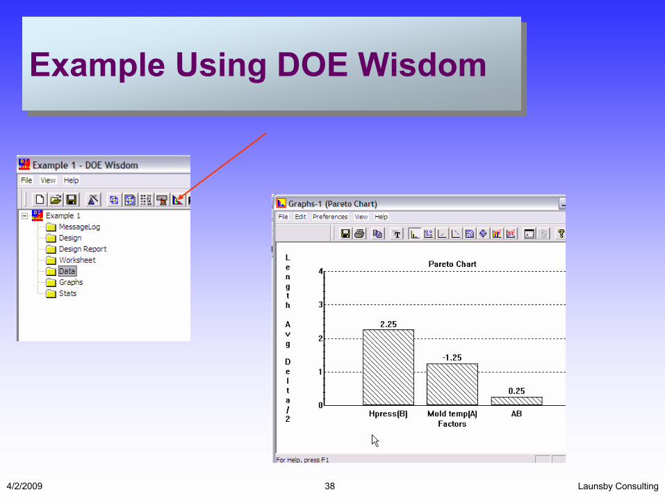
Pareto ChartPareto Chart
0
1
2
3
4
Hold press(B)
2.25
Mold temp(A)
-1.25
AB
0.25
Factors
Pareto ChartLength Avg Delta/2
Launsby Consulting4/2/2009 27
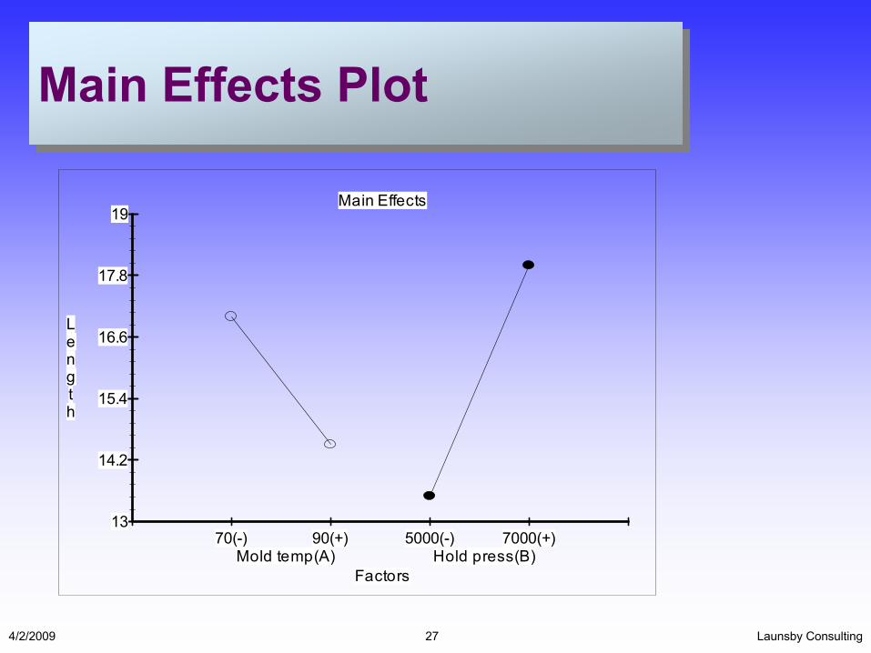
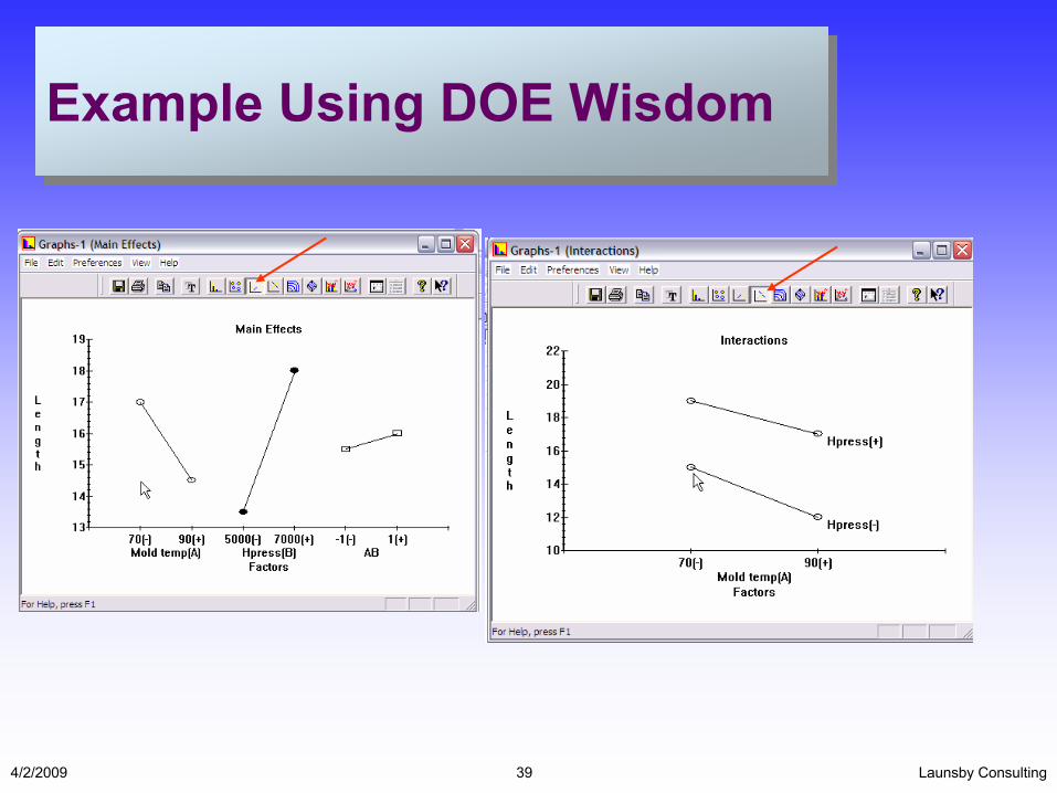
Main Effects PlotMain Effects Plot
13
14.2
15.4
16.6
17.8
19
70(-) 90(+)Mold temp(A)
5000(-) 7000(+)Hold press(B)
Factors
Main Effects
Length

Launsby Consulting4/2/2009 28
Transfer FunctionTransfer Function
• The equation (algebraic)
• It comes from MLR• Three important assumptions
– Two levels– O.A.– Variables are on orthogonal scale
• The equation (algebraic)
• It comes from MLR• Three important assumptions
– Two levels– O.A.– Variables are on orthogonal scale
Software packages use MLR to generate transfer function

Launsby Consulting4/2/2009 29
MLR MathMLR Math
[ ] [ ]
=
=
++++=−
...
.........ˆ
12
2
1
0
1211222110
bbbb
YXXX
xxbxbxbbytt
β
β
=
ny
yyyy
Y
.
.4
3
2
1
−+++−+++−−−−
=1..1..1..11..1..1..11..1..1..11..1..1..1
X
includes factors (assumes 4 run previous example), and interaction effect
Note: the computer does the math, we just need to be able to interpret the output
Launsby Consulting4/2/2009 30
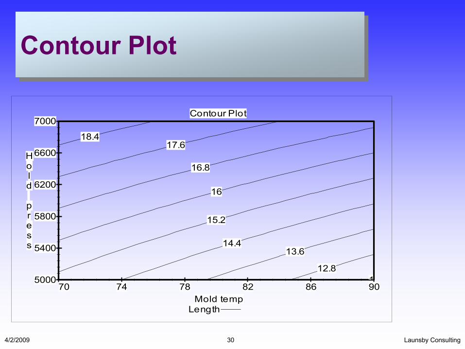
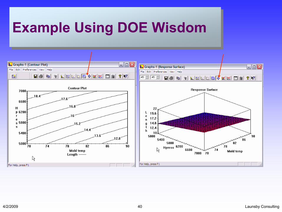
Contour PlotContour Plot
70 74 78 82 86 90Mold temp
5000
5400
5800
6200
6600
7000
Hold press
Contour Plot
Length
15.2
14.4
16
16.8
17.618.4
13.6
12.81
Launsby Consulting4/2/2009 31
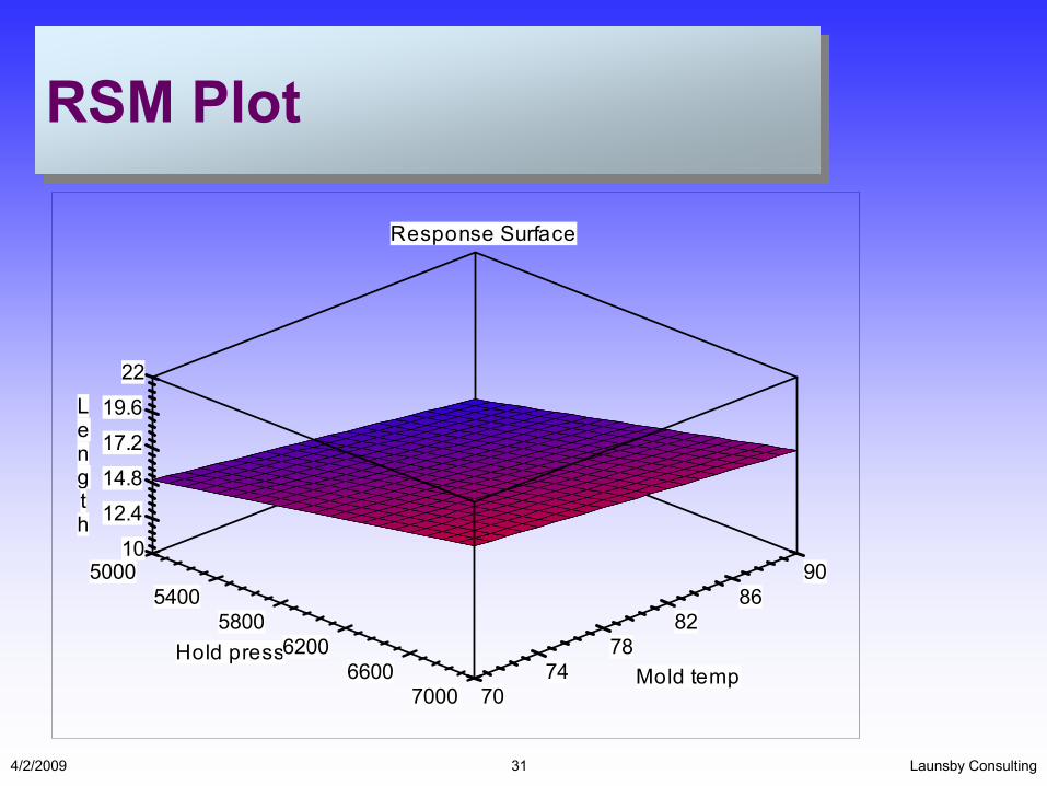
RSM PlotRSM Plot
Length
Hold pressMold temp
Response Surface
7074
7882
86905000
54005800
62006600
7000
10
12.4
14.8
17.2
19.6
22
Launsby Consulting4/2/2009 32
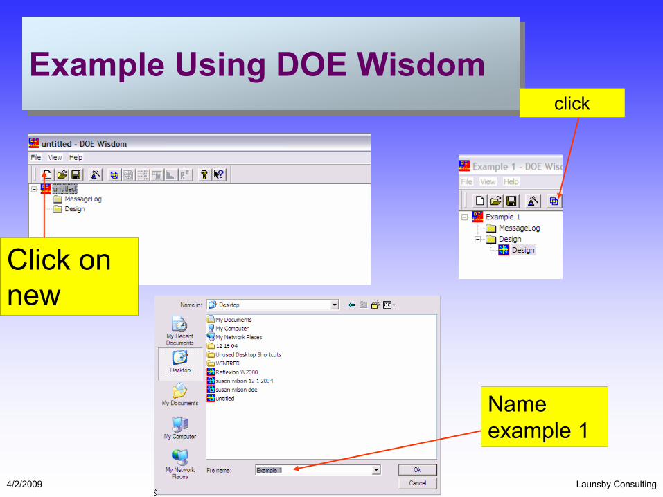
Example Using DOE WisdomExample Using DOE Wisdom
Click on new
Name example 1
click
Launsby Consulting4/2/2009 33
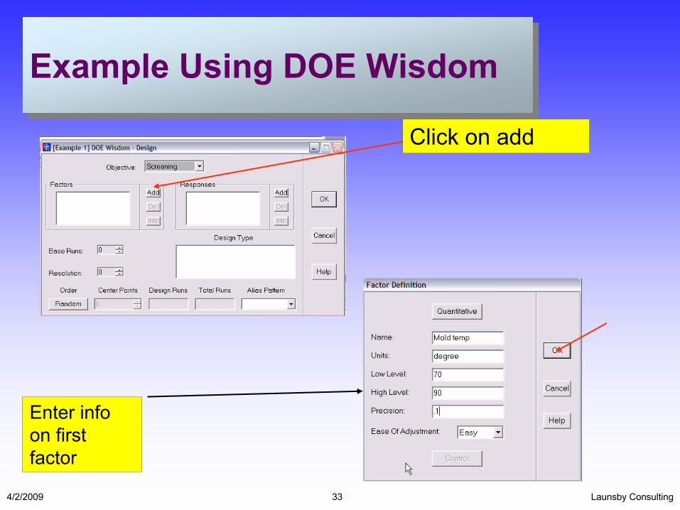
Example Using DOE WisdomExample Using DOE Wisdom
Click on add
Enter info on first factor
Launsby Consulting4/2/2009 34
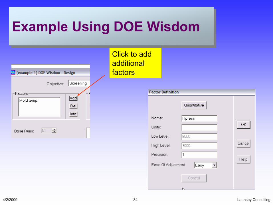
Example Using DOE WisdomExample Using DOE Wisdom
Click to add additional factors
Launsby Consulting4/2/2009 35
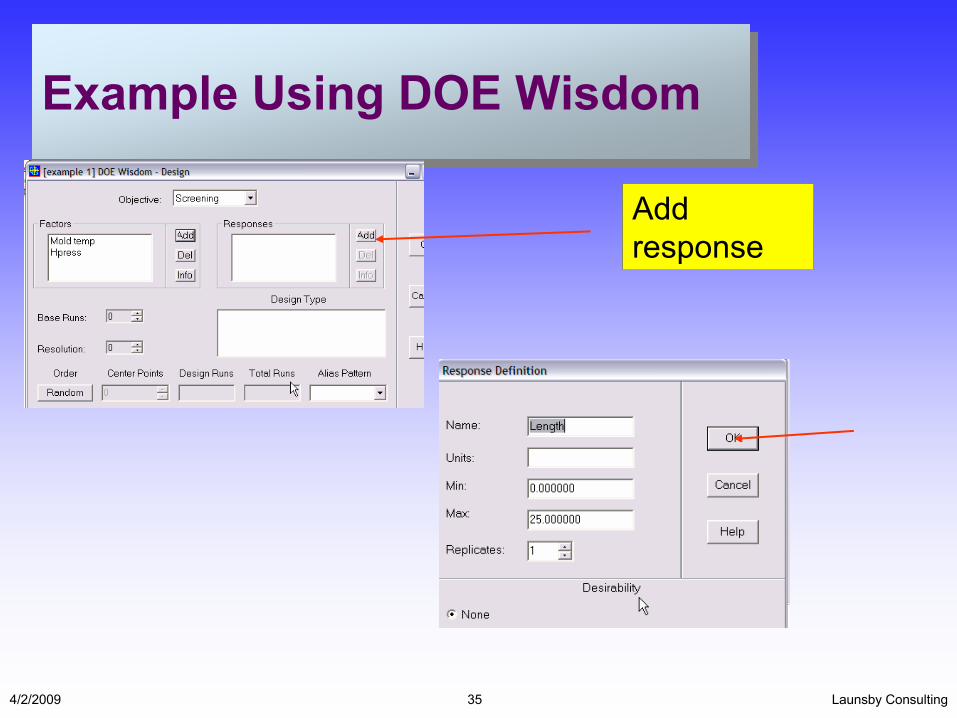
Example Using DOE WisdomExample Using DOE Wisdom
Add response

Launsby Consulting4/2/2009 36
Example Using DOE WisdomExample Using DOE Wisdom
select
Click when done

Launsby Consulting4/2/2009 37
Example Using DOE WisdomExample Using DOE Wisdom
Select data window
Enter data
Click save when done
Launsby Consulting4/2/2009 38
Example Using DOE WisdomExample Using DOE Wisdom
Launsby Consulting4/2/2009 39
Example Using DOE WisdomExample Using DOE Wisdom
Launsby Consulting4/2/2009 40
Example Using DOE WisdomExample Using DOE Wisdom

Launsby Consulting4/2/2009 41
Experimental ObjectivesExperimental Objectives
Launsby Consulting M12004 42
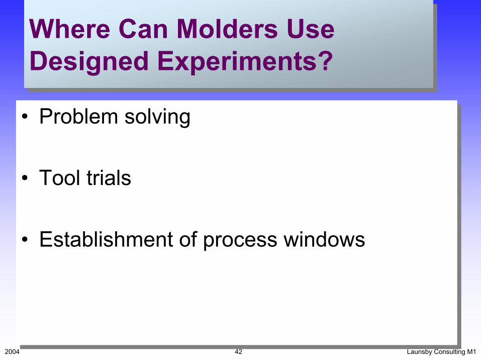
Where Can Molders Use Designed Experiments?Where Can Molders Use Designed Experiments?
• Problem solving
• Tool trials
• Establishment of process windows
• Problem solving
• Tool trials
• Establishment of process windows

Launsby Consulting4/2/2009 43
Troubleshooting/screeningTroubleshooting/screening

Launsby Consulting4/2/2009 44
Troubleshooting/screeningTroubleshooting/screening
FACTORS LOW HIGH Mold Temp 100 150 Barrel Temp Low High Cure Time 40 50 Back Press 50 150 Inj Velocity 1 3.1 Hold Press 200 1100

Launsby Consulting4/2/2009 45
Troubleshooting/screeningTroubleshooting/screening
• Response– Appearance– Decreasing shape– Rate as 1, 2, 3 (3 is best)
• O.A.– L8 with 5 repetitions
• Response– Appearance– Decreasing shape– Rate as 1, 2, 3 (3 is best)
• O.A.– L8 with 5 repetitions

Launsby Consulting4/2/2009 46
Main EffectsMain Effects
0
1
2
3
4
5
moldt barrelt injvel ctime holdp bckpreFactors
appear
Mold temp is big hitter, set at high for best appearance. Other factors appear to have little impact on appearance
Launsby Consulting4/2/2009 47
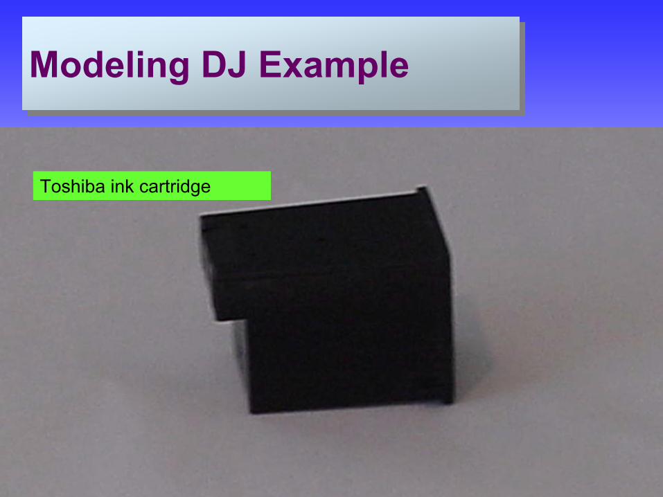
Modeling DJ ExampleModeling DJ Example
Toshiba ink cartridge

Launsby Consulting M12004 48
DJ ExampleDJ Example
FACTOR LOW HIGH
Hold Pressure (psi) 5000 8500
Pack Speed (%) 15 30
Injection Vel. (%) 30 65Mold Temp (deg.) 100 150
Launsby Consulting M12004 49
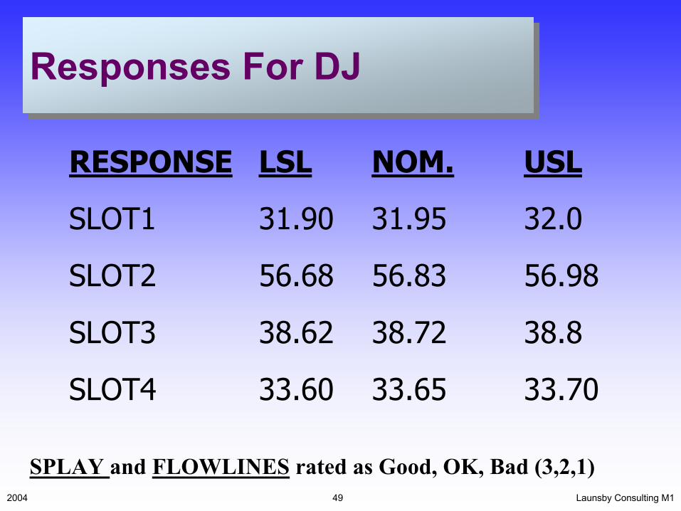
Responses For DJResponses For DJ
RESPONSE LSL NOM. USL
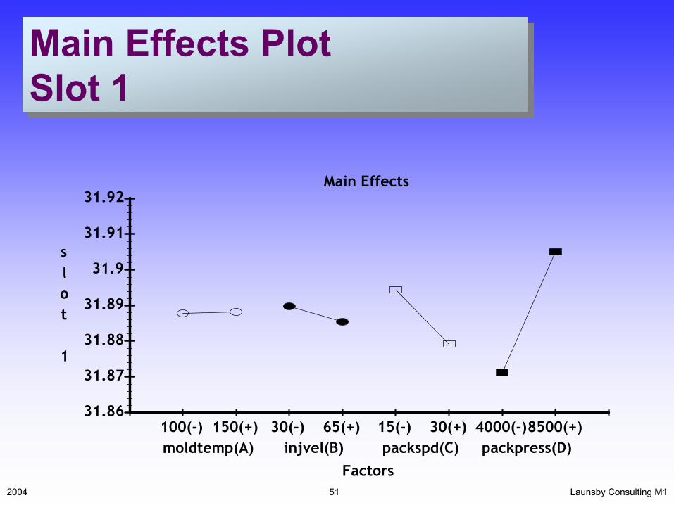
SLOT1 31.90 31.95 32.0
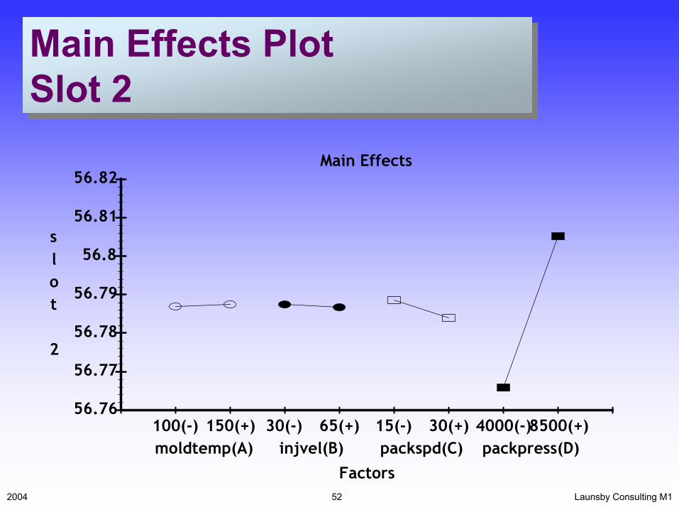
SLOT2 56.68 56.83 56.98
SLOT3 38.62 38.72 38.8
SLOT4 33.60 33.65 33.70
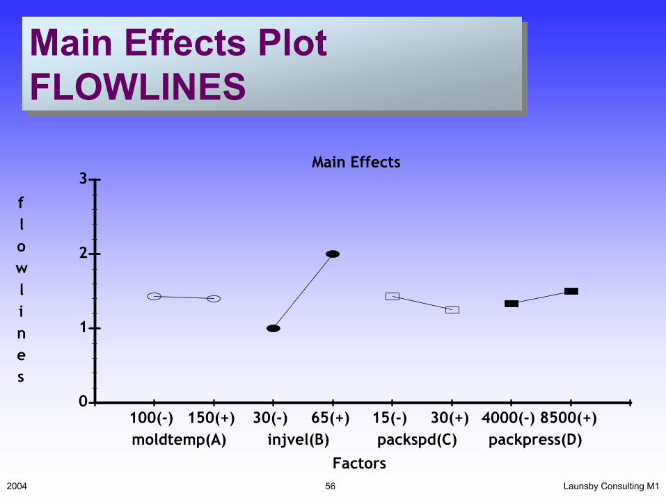
SPLAY and FLOWLINES rated as Good, OK, Bad (3,2,1)
Launsby Consulting M12004 50
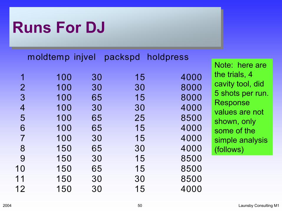
Runs For DJRuns For DJ
moldtemp injvel packspd holdpress
1 100 30 15 40002 100 30 30 80003 100 65 15 80004 100 30 30 40005 100 65 25 85006 100 65 15 40007 100 30 15 40008 150 65 30 40009 150 30 15 8500
10 150 65 15 850011 150 30 30 850012 150 30 15 4000
Note: here are the trials, 4 cavity tool, did 5 shots per run. Response values are not shown, only some of the simple analysis (follows)
Launsby Consulting M12004 51
Main Effects PlotSlot 1Main Effects PlotSlot 1
31.86
31.87
31.88
31.89
31.9
31.91
31.92
100(-) 150(+)moldtemp(A)
30(-) 65(+)injvel(B)
15(-) 30(+)packspd(C)
4000(-)8500(+)packpress(D)
Factors
Main Effects
slot 1
Launsby Consulting M12004 52
Main Effects Plot Slot 2Main Effects Plot Slot 2
56.76
56.77
56.78
56.79
56.8
56.81
56.82
100(-) 150(+)moldtemp(A)
30(-) 65(+)injvel(B)
15(-) 30(+)packspd(C)
4000(-)8500(+)packpress(D)
Factors
Main Effects
slot 2

Launsby Consulting M12004 53
Main Effects PlotSlot 3Main Effects PlotSlot 3
38.6
38.62
38.64
38.66
38.68
38.7
38.72
100(-) 150(+)moldtemp(A)
30(-) 65(+)injvel(B)
15(-) 30(+)packspd(C)
4000(-)8500(+)packpress(D)
Factors
Main Effects
slot 3

Launsby Consulting M12004 54
Main Effects PlotSlot 4Main Effects PlotSlot 4
33.57
33.58
33.59
33.6
33.61
33.62
33.63
100(-) 150(+)moldtemp(A)
30(-) 65(+)injvel(B)
15(-) 30(+)packspd(C)
4000(-)8500(+)packpress(D)
Factors
Main Effects
slot 4

Launsby Consulting M12004 55
Main Effects PlotSplayMain Effects PlotSplay
2.2
2.4
2.6
2.8
3
3.2
3.4
100(-) 150(+)moldtemp(A)
30(-) 65(+)injvel(B)
15(-) 30(+)packspd(C)
4000(-) 8500(+)packpress(D)
Factors
Main Effects
splay
Launsby Consulting M12004 56
Main Effects PlotFLOWLINESMain Effects PlotFLOWLINES
0
1
2
3
100(-) 150(+)moldtemp(A)
30(-) 65(+)injvel(B)
15(-) 30(+)packspd(C)
4000(-) 8500(+)packpress(D)
Factors
Main Effects
flowlines

Launsby Consulting M12004 57
What Is The Best Trade-off?What Is The Best Trade-off?
D(composite)
injvelmoldtemp
Response Surface**packspd(C)=15.0000,packpress(D)=7920.00
100
110
120
130
140
15030
37
44
51
58
65
0
0.1
0.2
0.3
0.4
Operate in this region

Launsby Consulting M12004 58
Slot 1 Slot 2 Slot 3 Slot 4
. . . .
PICTURAL View Of Trade-off (means)PICTURAL View Of Trade-off (means)
Note: slot 1 and slot 2 work the opposite of slots 3 and 4. Ifwe attempt to increase slot 1 and slot 2, slots 3 and slots 4 decrease. Good time to find this out is during tool trial

How About Variation?How About Variation?
Launsby Consulting M12004 59
Monte Carlo Simulation can be used to predict variation about a process meanDOE Wisdom Analysis of Variance
Dependent Variable: response 4Number Runs(N): 12Multiple R: 0.999807Squared Multiple R: 0.999614Adjusted Squared Multiple R: 0.995757Standard Error of Estimate: 0.000848528
Variable Coefficient best settingConstant 33.5985Mold Temp(A) 0.00506435 150Inj Vel(B) -0.00941707 47Pack Spd(C) -0.00507645 15Pack Prs(D) -0.00436898 7920AB 0.00572135AC 0.00363698AD -0.000393981BC -0.00360833BD -0.00193009CD -0.00225509
How closely can the factors be controlled in production?
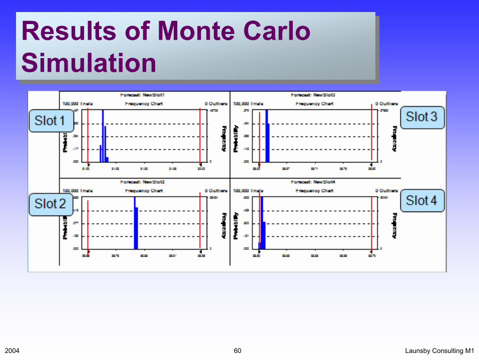
Results of Monte Carlo SimulationResults of Monte Carlo Simulation
Launsby Consulting M12004 60
Launsby Consulting4/2/2009 61
ROBUST DESIGNProduct LevelROBUST DESIGNProduct Level• What it Means
– Products Perform Intended Functions at Varying Usage Conditions
– Wide Range Customer Usage– Product Deterioration– Variation in Subsystems/Components
• What it Means– Products Perform Intended Functions at
Varying Usage Conditions– Wide Range Customer Usage– Product Deterioration– Variation in Subsystems/Components
Launsby Consulting4/2/2009 62
Robustness At The Process LevelRobustness At The Process Level• Lot-to-Lot Variation in Resin• Regrind• Machine• Room Temperature• Moisture Content• Operator
• Lot-to-Lot Variation in Resin• Regrind• Machine• Room Temperature• Moisture Content• Operator
Launsby Consulting4/2/2009 63
Robust Design(Cont.)Robust Design(Cont.)• Robust Design Recognizes That Variability
Exists and is the Enemy of High Quality Products and Processes
• Employs DOE as a Strategic Weapon• Accomplished by Selecting the Best Levels
for Control Factors so That Performance Insensitive to Noise Factors
• Robust Design Recognizes That Variability Exists and is the Enemy of High Quality Products and Processes
• Employs DOE as a Strategic Weapon• Accomplished by Selecting the Best Levels
for Control Factors so That Performance Insensitive to Noise Factors

Launsby Consulting4/2/2009 64
Robust Design(Examples)Robust Design(Examples)• Caramel Candy Example
• Industry Examples (HP Ink Cartridge…see following slides)
• Caramel Candy Example
• Industry Examples (HP Ink Cartridge…see following slides)

Launsby Consulting4/2/2009 65
HP weld exampleHP weld example
Launsby Consulting4/2/2009 66
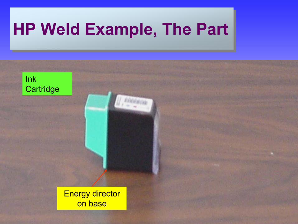
HP Weld Example, The PartHP Weld Example, The Part
Ink Cartridge
Energy director on base
Launsby Consulting4/2/2009 67
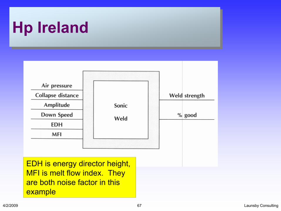
Hp IrelandHp Ireland
EDH is energy director height, MFI is melt flow index. They are both noise factor in this example
Launsby Consulting4/2/2009 68
Robust Design ExampleRobust Design Example
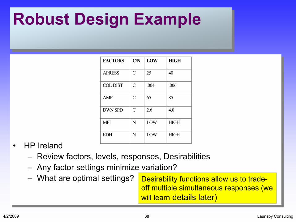
• HP Ireland– Review factors, levels, responses, Desirabilities– Any factor settings minimize variation?– What are optimal settings?
• HP Ireland– Review factors, levels, responses, Desirabilities– Any factor settings minimize variation?– What are optimal settings?
FACTORS C/N LOW HIGH
APRESS C 25 40
COL DIST C .004 .006
AMP C 65 85
DWN SPD C 2.6 4.0
MFI N LOW HIGH
EDH N LOW HIGH
Desirability functions allow us to trade-off multiple simultaneous responses (we will learn details later)
Launsby Consulting4/2/2009 69
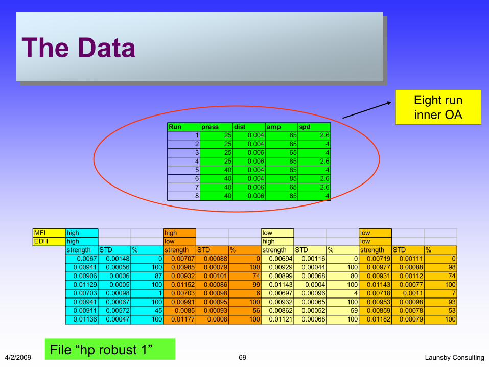
Run press dist amp spd1 25 0.004 65 2.62 25 0.004 85 43 25 0.006 65 44 25 0.006 85 2.65 40 0.004 65 46 40 0.004 85 2.67 40 0.006 65 2.68 40 0.006 85 4
high high low lowhigh low high lowstrength STD % strength STD % strength STD % strength STD %
0.0067 0.00148 0 0.00707 0.00088 0 0.00694 0.00116 0 0.00719 0.00111 00.00941 0.00056 100 0.00985 0.00079 100 0.00929 0.00044 100 0.00977 0.00088 980.00906 0.0006 87 0.00932 0.00101 74 0.00899 0.00068 80 0.00931 0.00112 740.01129 0.0005 100 0.01152 0.00086 99 0.01143 0.0004 100 0.01143 0.00077 1000.00703 0.00098 1 0.00703 0.00098 6 0.00697 0.00096 4 0.00718 0.0011 70.00941 0.00067 100 0.00991 0.00095 100 0.00932 0.00065 100 0.00953 0.00098 930.00911 0.00572 45 0.0085 0.00093 56 0.00862 0.00052 59 0.00859 0.00078 530.01136 0.00047 100 0.01177 0.0008 100 0.01121 0.00068 100 0.01182 0.00079 100
MFIEDH
The DataThe Data
File “hp robust 1”
Eight run inner OA

Launsby Consulting4/2/2009 70
Robust Design, StrengthRobust Design, Strength
0.006
0.007
0.008
0.009
0.01
0.011
0.012
25(-) 40(+)press(A)
0.004(-) 0.006(+)dist(B)
65(-) 85(+)amp(C)
2.6(-) 4(+)spd(D)
Factors
Main Effects
strength
Average

Launsby Consulting4/2/2009 71
Robust Design (Cont.)Robust Design (Cont.)
• Students: What is the best trade-off?• Students: What is the best trade-off?
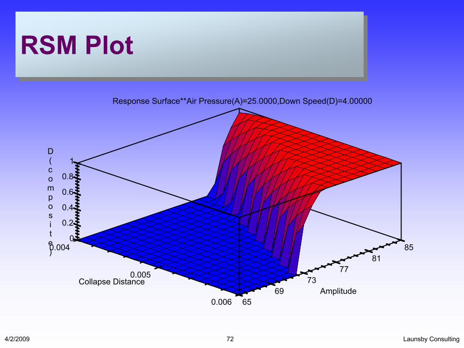
Mean (Weld Str) Stand Dev (Weld Str) % Good Welds D(composite)0.0116059 0.00044375 122.25 1
95% CI: ± 0.000498452 ± 0.00193891 ± 39.7551Constant 0.00924781 0.000975 66.75Air Pressure(A) -3.78E-05 0.0001475 -2.75 25Collapse Distance(B) 0.000960313 6.44E-05 16.1875 0.006Amplitude(C) 0.00127219 -0.000275625 32.625 85Down Speed(D) 8.78E-05 -0.0001725 3.9375 4
Here are the predicted optimal setting for factors
Launsby Consulting4/2/2009 72
RSM PlotRSM Plot
D(composite)
Collapse DistanceAmplitude
Response Surface**Air Pressure(A)=25.0000,Down Speed(D)=4.00000
6569
7377
81850.004
0.005
0.006
0
0.2
0.4
0.6
0.8
1

Launsby Consulting4/2/2009 73
Knowledge Of The Technology To Enhance RobustnessKnowledge Of The Technology To Enhance Robustness
• Viscosity vs. Shear Curves
• Cavity Pressure Sensors
• Viscosity vs. Shear Curves
• Cavity Pressure Sensors
Cavity pressure changes are a major source of dimensional and appearance variation

Launsby Consulting4/2/2009 74
Conventional MoldingConventional Molding
• Fill and Pack are Done on First Stage• Time is Usually Used to Transfer From
Boost to Hold
• Fill and Pack are Done on First Stage• Time is Usually Used to Transfer From
Boost to Hold

Launsby Consulting4/2/2009 75
Typical Pressure ProfileTypical Pressure Profile
From “Plastic Part Design” by R.A. Malloy

Launsby Consulting4/2/2009 76
Hydraulic Pressure Is MisleadingHydraulic Pressure Is Misleading
Source: RJG, Inc.
Hydraulic Injection Pressure
Mold Cavity Pressure
Launsby Consulting4/2/2009 77
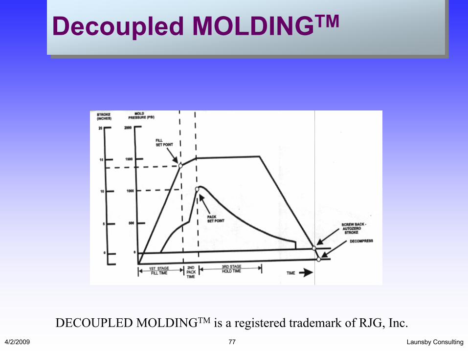
Decoupled MOLDINGTMDecoupled MOLDINGTM
DECOUPLED MOLDINGTM is a registered trademark of RJG, Inc.

Launsby Consulting4/2/2009 78
Cavity Pressure ImpactCavity Pressure Impact
Source: RJG, Inc.

Launsby Consulting4/2/2009 79
Cavity Control ImpactCavity Control Impact
MOLDINGTECHNIQUE
GATE ENDMOLDPRESS (s.d.)
EOF MOLDPRESS (s.d.)
Traditional 514 860
TotallyDecoupled
21.4 205
Source: RJG Associates, Decoupled Molding is a Trademark of RJG in Traverse City, MI
Launsby Consulting4/2/2009 80
Box And Bubble ChartBox And Bubble Chart
• Planning• Select an Orthogonal Array• Conduct • Analysis• Confirmation
• Planning• Select an Orthogonal Array• Conduct • Analysis• Confirmation

Launsby Consulting4/2/2009 81
PlanningPlanning
• Who Are the Customers?• How Will Customers Use Products?• What are the Functions?• Objectives?• Time Requirements• Responses, Factors, Money
• Who Are the Customers?• How Will Customers Use Products?• What are the Functions?• Objectives?• Time Requirements• Responses, Factors, Money
Launsby Consulting4/2/2009 82
Orthogonal ArrayOrthogonal Array
• A Set of Experimental Conditions (runs) Where the Levels of Each Factors are Balanced Over the Levels of the Other Factors, Both Horizontally and Vertically
• A Balanced Family of Tests Which Allows For Fast, Efficient, Simple, and Powerful Analysis
• Example-----Golf
• A Set of Experimental Conditions (runs) Where the Levels of Each Factors are Balanced Over the Levels of the Other Factors, Both Horizontally and Vertically
• A Balanced Family of Tests Which Allows For Fast, Efficient, Simple, and Powerful Analysis
• Example-----Golf
Launsby Consulting4/2/2009 83
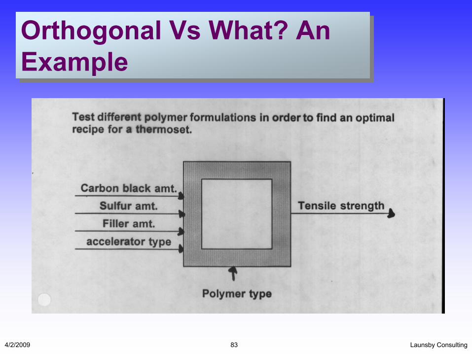
Orthogonal Vs What? An ExampleOrthogonal Vs What? An Example
Launsby Consulting4/2/2009 84
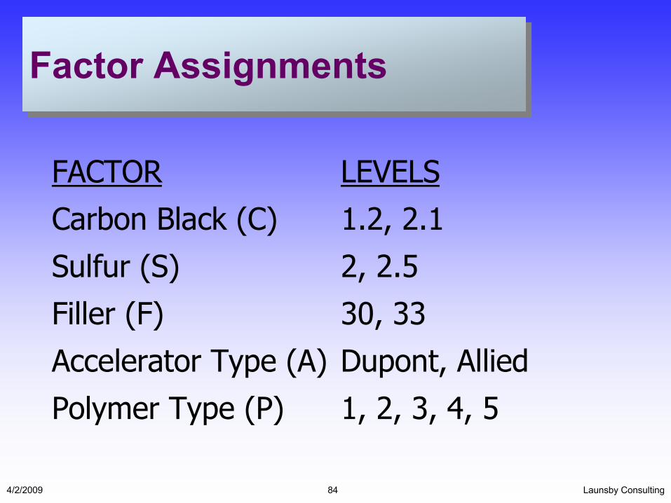
Factor AssignmentsFactor Assignments
FACTOR LEVELSCarbon Black (C) 1.2, 2.1Sulfur (S) 2, 2.5Filler (F) 30, 33Accelerator Type (A) Dupont, AlliedPolymer Type (P) 1, 2, 3, 4, 5
Launsby Consulting4/2/2009 85
Full FactorialApproachFull FactorialApproach• Advantages
• Disadvantages
• Advantages
• Disadvantages
Launsby Consulting4/2/2009 86
One-factor-atA TimeOne-factor-atA Time• Advantages
• Disadvantages
• Advantages
• Disadvantages
Launsby Consulting4/2/2009 87
Best Guess ApproachBest Guess Approach
• Advantages
• Disadvantages
• Advantages
• Disadvantages

Launsby Consulting4/2/2009 88
Experimentation InThe 00’sExperimentation InThe 00’s• Full Factorials, Taguchi O.A.’s• Fractional-Factorials• Plackett-Burman• Hadamard Matrices• Box-Behnken, Central Composite• D-optimal Designs
• Full Factorials, Taguchi O.A.’s• Fractional-Factorials• Plackett-Burman• Hadamard Matrices• Box-Behnken, Central Composite• D-optimal Designs

Launsby Consulting4/2/2009 89
Module #2Module #2
• Goals– Understand the Steps Required for Success– Set-up and Analyze a Simple Design– Learn When Analysis is Unsuccessful and
Grasp How to Recover– Apply Desirability Functions (using software).
• Goals– Understand the Steps Required for Success– Set-up and Analyze a Simple Design– Learn When Analysis is Unsuccessful and
Grasp How to Recover– Apply Desirability Functions (using software).
Launsby Consulting4/2/2009 90
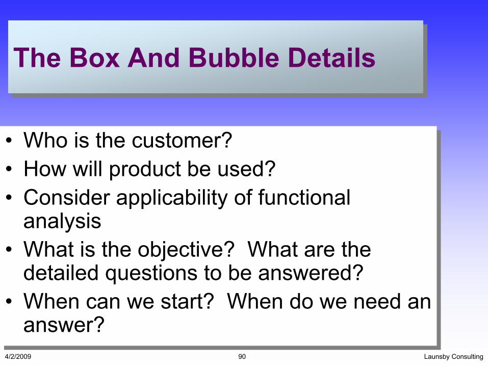
The Box And Bubble DetailsThe Box And Bubble Details
• Who is the customer?• How will product be used?• Consider applicability of functional
analysis• What is the objective? What are the
detailed questions to be answered?• When can we start? When do we need an
answer?
• Who is the customer?• How will product be used?• Consider applicability of functional
analysis• What is the objective? What are the
detailed questions to be answered?• When can we start? When do we need an
answer?

Launsby Consulting4/2/2009 91
The Box And Bubble Details (Cont)The Box And Bubble Details (Cont)• Responses
– Name, how measured?, MSA?, shape, critical values, weight
• Factors– Name, qualitative or quantitative? Range of
interest, levels, propensity for interactions• Costs
– Approximate cost per run, time per run
• Responses– Name, how measured?, MSA?, shape, critical
values, weight• Factors
– Name, qualitative or quantitative? Range of interest, levels, propensity for interactions
• Costs– Approximate cost per run, time per run
Launsby Consulting4/2/2009 92
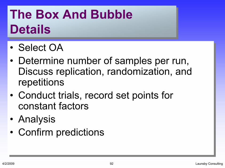
The Box And Bubble DetailsThe Box And Bubble Details• Select OA• Determine number of samples per run,
Discuss replication, randomization, and repetitions
• Conduct trials, record set points for constant factors
• Analysis• Confirm predictions
• Select OA• Determine number of samples per run,
Discuss replication, randomization, and repetitions
• Conduct trials, record set points for constant factors
• Analysis• Confirm predictions

Launsby Consulting4/2/2009 93
Four Types Of FactorsFour Types Of Factors
• Effect Location
• Effect Variation
• Effect Both
• No Effect
• Effect Location
• Effect Variation
• Effect Both
• No Effect
Launsby Consulting4/2/2009 94
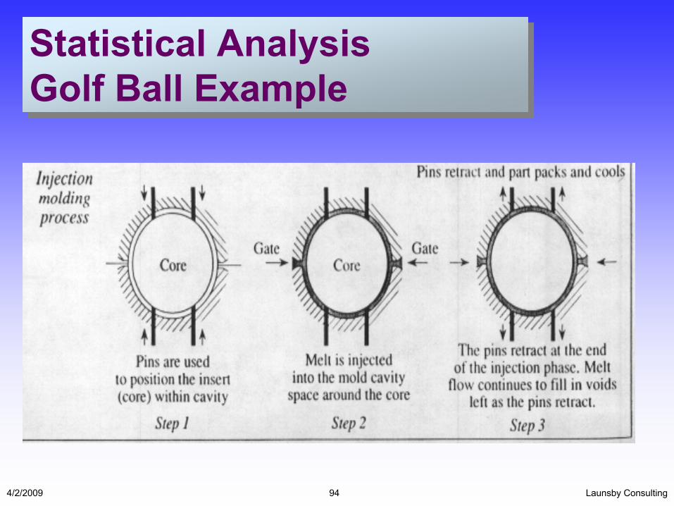
Statistical AnalysisGolf Ball ExampleStatistical AnalysisGolf Ball Example

Launsby Consulting4/2/2009 95
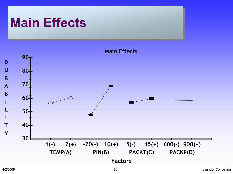
Introduction To Simple AnalysisIntroduction To Simple Analysis
Run TEMP PIN PACKT PACKP1 1 -20 5 6002 1 -20 15 9003 1 10 5 9004 1 10 15 6005 2 -20 5 9006 2 -20 15 6007 2 10 5 6008 2 10 15 900
DURA.4547646949496974
WT44.845.345.344.845.444.944.945.4
Launsby Consulting4/2/2009 96
Main EffectsMain Effects
30
40
50
60
70
80
90
1(-) 2(+)TEMP(A)
-20(-) 10(+)PIN(B)
5(-) 15(+)PACKT(C)
600(-) 900(+)PACKP(D)
Factors
Main Effects
DURABILITY

Launsby Consulting4/2/2009 97
Main EffectsMain Effects
44.8
44.9
45
45.1
45.2
45.3
45.4
1(-) 2(+)TEMP(A)
-20(-) 10(+)PIN(B)
5(-) 15(+)PACKT(C)
600(-) 900(+)PACKP(D)
Factors
Main Effects
WEIGHT

Launsby Consulting4/2/2009 98
Stats AnalysisWeightStats AnalysisWeight
DOE Wisdom Analysis of Variance
Dependent Variable: WEIGHTNumber Runs(N): 128Multiple R: 0.963484Squared Multiple R: 0.928301Adjusted Squared Mu 0.925969Standard Error of Esti 0.067707
Variable Coefficient Std Error 95% CI Tolerance T P(2 Tail)
Constant 45.1056 0.005985 ± 0.0118460 7537.012 0TEMP(A) 0.048281 0.005985 ± 0.011846 1 8.068 0PIN(B) -0.0025 0.005985 ± 0.011846 1 -0.418 0.677PACKT(C) 0.007656 0.005985 ± 0.011846 1 1.279 0.203PACKP(D) 0.23375 0.005985 ± 0.011846 1 39.059 0
Launsby Consulting4/2/2009 99
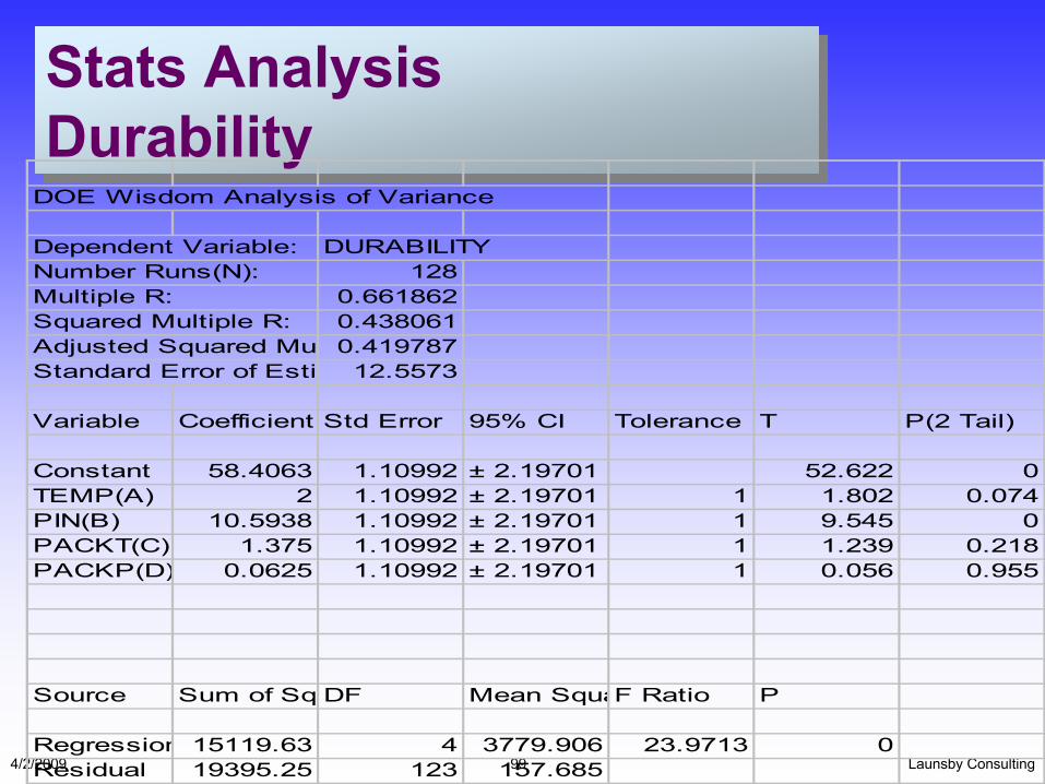
Stats AnalysisDurabilityStats AnalysisDurability
DOE Wisdom Analysis of Variance
Dependent Variable: DURABILITYNumber Runs(N): 128Multiple R: 0.661862Squared Multiple R: 0.438061Adjusted Squared Mu 0.419787Standard Error of Esti 12.5573
Variable Coefficient Std Error 95% CI Tolerance T P(2 Tail)
Constant 58.4063 1.10992 ± 2.19701 52.622 0TEMP(A) 2 1.10992 ± 2.19701 1 1.802 0.074PIN(B) 10.5938 1.10992 ± 2.19701 1 9.545 0PACKT(C) 1.375 1.10992 ± 2.19701 1 1.239 0.218PACKP(D) 0.0625 1.10992 ± 2.19701 1 0.056 0.955
Source Sum of Sq DF Mean SquaF Ratio P
Regression 15119.63 4 3779.906 23.9713 0Residual 19395.25 123 157.685

Launsby Consulting4/2/2009 100
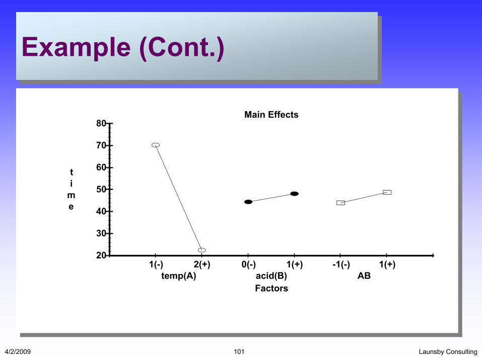
Example Example
Run temp acid time time time time time time time1 1 0 67 79 71 73 69 65 702 1 1 66 71 81 67 68 73 613 2 0 17 22 18 19 17 17 174 2 1 26 26.5 25.5 27 28 27 26.6
Launsby Consulting4/2/2009 101
Example (Cont.)Example (Cont.)
20
30
40
50
60
70
80
1(-) 2(+)temp(A)
0(-) 1(+)acid(B)
-1(-) 1(+)AB
Factors
Main Effects
ti
me
Launsby Consulting4/2/2009 102
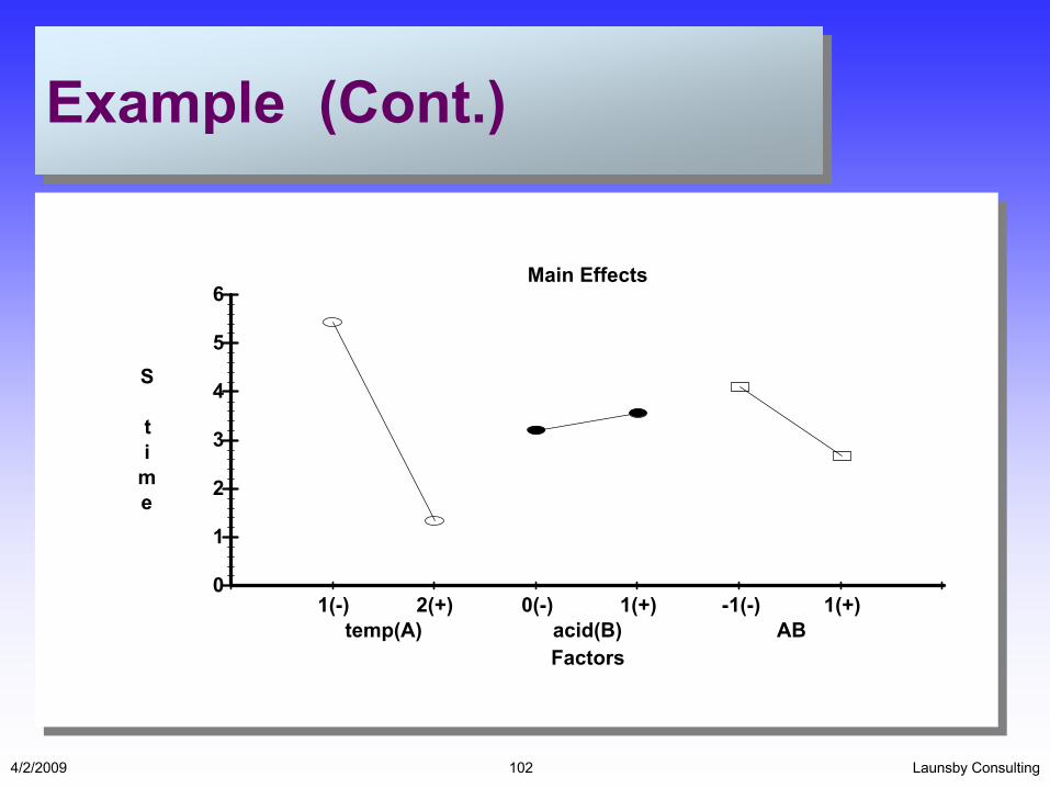
Example (Cont.)Example (Cont.)
0
1
2
3
4
5
6
1(-) 2(+)temp(A)
0(-) 1(+)acid(B)
-1(-) 1(+)AB
Factors
Main Effects
S ti
me
Launsby Consulting4/2/2009 103
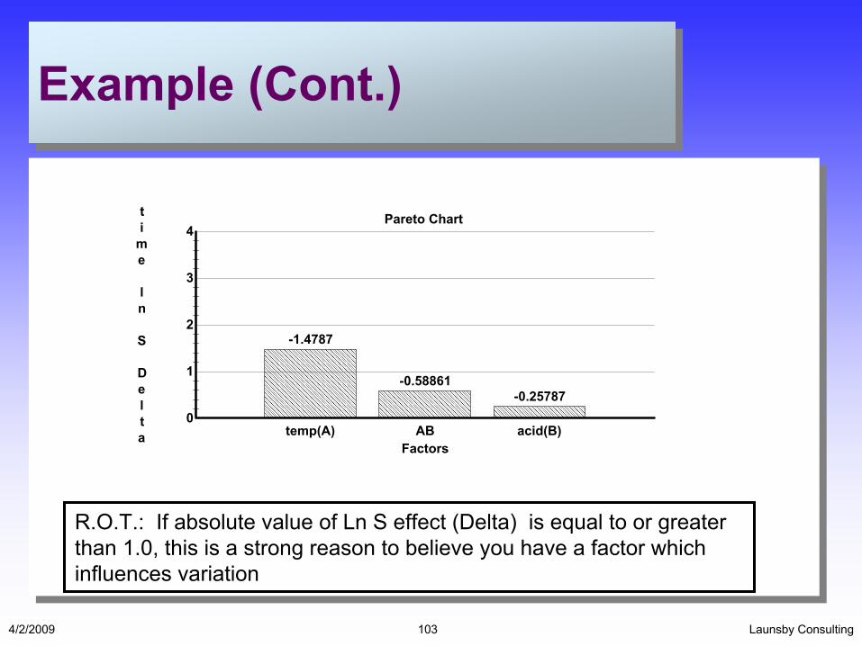
Example (Cont.)Example (Cont.)
R.O.T.: If absolute value of Ln S effect (Delta) is equal to or greater than 1.0, this is a strong reason to believe you have a factor which influences variation
0
1
2
3
4
temp(A)
-1.4787
AB
-0.58861
acid(B)
-0.25787
Factors
Pareto Chartti
me ln S Delta

Launsby Consulting4/2/2009 104
Example #3Example #3
QUESTION: How The Tabled Taguchi Designs Differ From Fractional-Factorials?
Launsby Consulting4/2/2009 105
Example # 4Example # 4
• Important terms– Interaction Columns– Aliasing– Resolution
• Important terms– Interaction Columns– Aliasing– Resolution
Launsby Consulting4/2/2009 106
Tabled Taguchi DesignsTabled Taguchi Designs
See pages 52 thru 58 (Experimental Design for Injection Molding for L4, L8, L9, L16,…..)
Launsby Consulting4/2/2009 107
D-optimal DesignsD-optimal Designs
• Advantages
• Disadvantages
• Advantages
• Disadvantages
Launsby Consulting4/2/2009 108
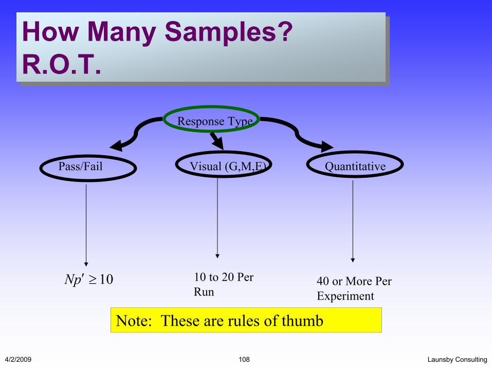
How Many Samples?R.O.T.How Many Samples?R.O.T.
Response Type
Pass/Fail Visual (G,M,E) Quantitative
40 or More Per Experiment
10 to 20 Per Run
10≥′pN
Note: These are rules of thumb

Launsby Consulting4/2/2009 109
How Many Samples?How Many Samples?
• Easy to provide if:– You have an estimate of the standard deviation
for response being studied– Know what is a practically significant difference
• Easy to provide if:– You have an estimate of the standard deviation
for response being studied– Know what is a practically significant difference

Launsby Consulting4/2/2009 110
Statistical SignificanceStatistical Significance
• People talk a great deal about statistical significance; yet spend almost no time regarding practical significance
• Reality– Any effect (as long as it is not zero) will be shown as
statistically significant if enough samples are used– You can mathematically justify any sample size by
tweaking inputs to formula

Launsby Consulting4/2/2009 111
Statistical/Practical SignificanceStatistical/Practical Significance
Variable Coefficient Std Error 95% CI Tolerance T P(2 Tail)
Constant 17.0505 0.201485 ± 0.464627 84.624 0 tech(A):A 1.06016 0.209227 ± 0.482480 5.067 0.001 tech(A):B -1.06016 0.209227 ± 0.482480 0.888 -5.067 0.001(B) 0.689843 0.209227 ± 0.482480 0.888 3.297 0.011(C) 0.796313 0.226216 ± 0.521657 0.908 3.52 0.008(D) -0.915697 0.249362 ± 0.575030 0.875 -3.672 0.006
All are statistically significant
If the difference is not greater than 4, it is not of practical importance
Not a big deal
Need both before you get very excited
14
15
16
17
18
19
20
A(-) B(+)(A)
1(-) 2(+)(B)
3(-) 5(+)(C)
2(-) 4(+)(D)
Factors
Main Effects
bump ht

Launsby Consulting4/2/2009 112
Sample Size For Mean Shift (one approach)Sample Size For Mean Shift (one approach)
===
=
σλ
λσ
n
n
2
162
2
Total number of samples in experiment
Minimum practical difference we wish to find as significant
Error standard deviation
Example: We decide to conduct an L8. We decide that 4 and estimate the error standard deviation as 4. The number of samples for the experiment is 32. We need to run the L8 4 times.
=λ
222
222
/)22(302
/)(
λσ
βα
λσβα
+≈
≥==
+=
nn
ttn.02
.02

Launsby Consulting4/2/2009 113
ConfirmationConfirmation
• Recommended # of Tests
• Graphical Approach
• Recommended # of Tests
• Graphical Approach

Launsby Consulting4/2/2009 114
Why You May Not ConfirmWhy You May Not Confirm• Data Entry• Did Not Conduct Per Plan• Measurement System Not Reliable• Large Variation in the Response• Wrong About Interactions• Model is Inadequate• Something Changed (Viscosity)• “Computer On/Brain Off”
• Data Entry• Did Not Conduct Per Plan• Measurement System Not Reliable• Large Variation in the Response• Wrong About Interactions• Model is Inadequate• Something Changed (Viscosity)• “Computer On/Brain Off”

Launsby Consulting4/2/2009 115
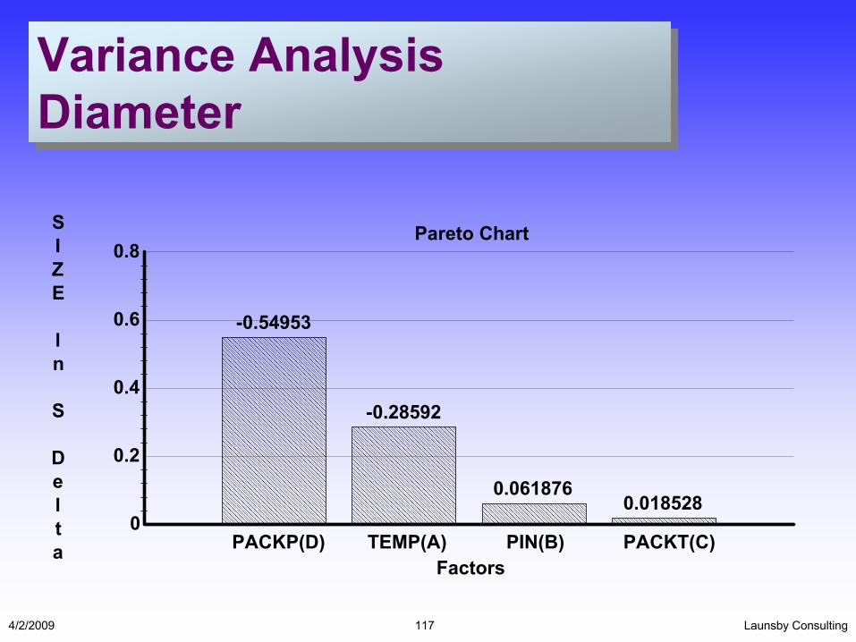
Golf ExampleAnalysis Of DiameterGolf ExampleAnalysis Of Diameter• Which Factors Appear to be Influencing the
Average?• Do Any Factors Appear to be Influencing
the Variation in the Diameter?• How Should We Set the Process to
Achieve a Target Response of 1.682?
• Which Factors Appear to be Influencing the Average?
• Do Any Factors Appear to be Influencing the Variation in the Diameter?
• How Should We Set the Process to Achieve a Target Response of 1.682?
Note: please use following graphs to answer above questions

Launsby Consulting4/2/2009 116
Main EffectsDiameterMain EffectsDiameter
1.68
1.682
1.684
1.686
1.688
1.69
1.692
1(-) 2(+)TEMP(A)
-20(-) 10(+)PIN(B)
5(-) 15(+)PACKT(C)
600(-) 900(+)PACKP(D)
Factors
Main Effects
SIZE
Launsby Consulting4/2/2009 117
Variance AnalysisDiameterVariance AnalysisDiameter
0
0.2
0.4
0.6
0.8
PACKP(D)
-0.54953
TEMP(A)
-0.28592
PIN(B)
0.061876
PACKT(C)
0.018528
Factors
Pareto ChartSIZE ln S Delta

Launsby Consulting4/2/2009 118
Stats AnalysisDiameterStats AnalysisDiameter
DOE Wisdom Analysis of Variance
Dependent Variable: SIZENumber Runs(N): 128Multiple R: 0.918717Squared Multiple R: 0.844041Adjusted Squared Mu 0.838969Standard Error of Esti 0.001534
Variable Coefficient Std Error 95% CI Tolerance T P(2 Tail)
Constant 1.68614 0.000136 ± 0.000268335 12438.2 0TEMP(A) 0.000874 0.000136 ± 0.000268 1 6.447 0PIN(B) -0.00023 0.000136 ± 0.000268 1 -1.709 0.09PACKT(C) 8.33E-05 0.000136 ± 0.000268 1 0.614 0.54PACKP(D) 0.003378 0.000136 ± 0.000268 1 24.916 0
Source Sum of Sq DF Mean SquaF Ratio P
Regression 0.001566 4 0.000391 166.417 0Residual 0.000289 123 2.35E-06
Launsby Consulting4/2/2009 119
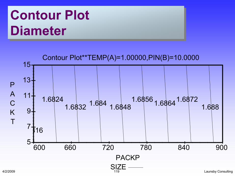
Contour PlotDiameterContour PlotDiameter
600 660 720 780 840 900PACKP
5
7
9
11
13
15
PACKT
Contour Plot**TEMP(A)=1.00000,PIN(B)=10.0000
SIZE
816
1.68241.6832 1.684 1.6848
1.68561.68641.68721.688

Launsby Consulting4/2/2009 120
Residual AnalysisResidual Analysis
• What is it?– A method for evaluating errors in model
predictions• What are the benefits?
– Check of model assumptions– Evaluation of model adequacy– Increased understanding of technology
• What patterns should emerge?
• What is it?– A method for evaluating errors in model
predictions• What are the benefits?
– Check of model assumptions– Evaluation of model adequacy– Increased understanding of technology
• What patterns should emerge?

Launsby Consulting4/2/2009 121
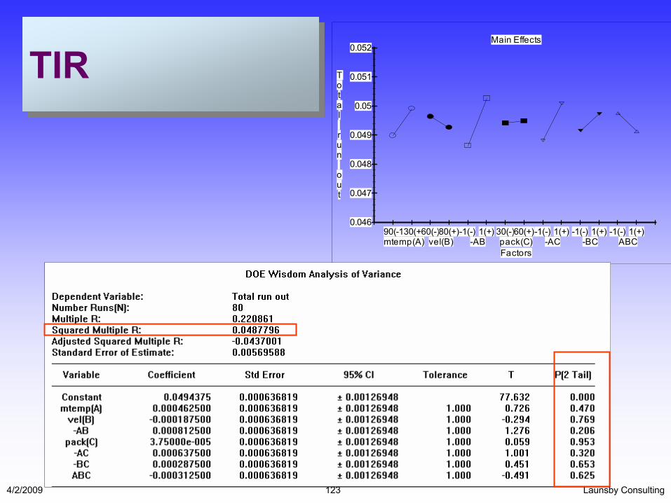
ExampleExample
• “Epsoon” (full-factorial, single cavity, 10 shots per run)
• “Epsoon” (full-factorial, single cavity, 10 shots per run)Factors LevelsMtemp 90, 130Injection Velocity 60, 80 %Pack Press 30, 60%
ResponsesDimension “E”Total run out

Launsby Consulting4/2/2009 122
Dim “E”Dim “E”
13.01
13.02
13.03
13.04
13.05
13.06
13.07
90(-)130(+)mtemp(A)
60(-)80(+)vel(B)
-1(-) 1(+)-AB
30(-)60(+)pack(C)
-1(-) 1(+)-AC
-1(-) 1(+)-BC
-1(-) 1(+)ABC
Factors
Main Effects
dimension E
Launsby Consulting4/2/2009 123
TIR TIR
0.046
0.047
0.048
0.049
0.05
0.051
0.052
90(-)130(+)mtemp(A)
60(-)80(+)vel(B)
-1(-) 1(+)-AB
30(-)60(+)pack(C)
-1(-) 1(+)-AC
-1(-) 1(+)-BC
-1(-) 1(+)ABC
Factors
Main Effects
Total run out

Launsby Consulting4/2/2009 124
EPSOON Dim “E” Student ResidualEPSOON Dim “E” Student Residual

Launsby Consulting4/2/2009 125
Dim “E” Student Residual PlotDim “E” Student Residual Plot
-4
-2
0
2
4
6
8
1234567891011121314151617181920212223242526272829303132333435363738394041424344454647484950515253545556575859606162636465666768697071727374757677787980R u n O r d e r
d
i
m
E
s
t
u
d
r
e
s
R e s i d u a l S c a t t e r P l o t

Launsby Consulting4/2/2009 126
TIR Student ResidualsTIR Student Residuals
0
2
4
6
8
10
-2.2
1
-2
0
-1.8
1
-1.6
2
-1.4
2
-1.2
9
-1
7
-0.8
4
-0.6
6
-0.4
2
-0.2
5
0
1
0.2
3
0.4
2
0.6
4
0.8
9
1
8
1.2
9
1.4
2
1.6
3
1.8
0
Total run out Studentized Residual
Count
Residual Histogram

Launsby Consulting4/2/2009 127
TIR Student ResidualsTIR Student Residuals
-3
-2
-1
0
1
2
3
1234567891011121314151617181920212223242526272829303132333435363738394041424344454647484950515253545556575859606162636465666768697071727374757677787980R u n O r d e r
r
u
n
o
u
t
s
t
u
d
r
e
s
l
R e s i d u a l S c a t t e r P l o t
Launsby Consulting4/2/2009 128
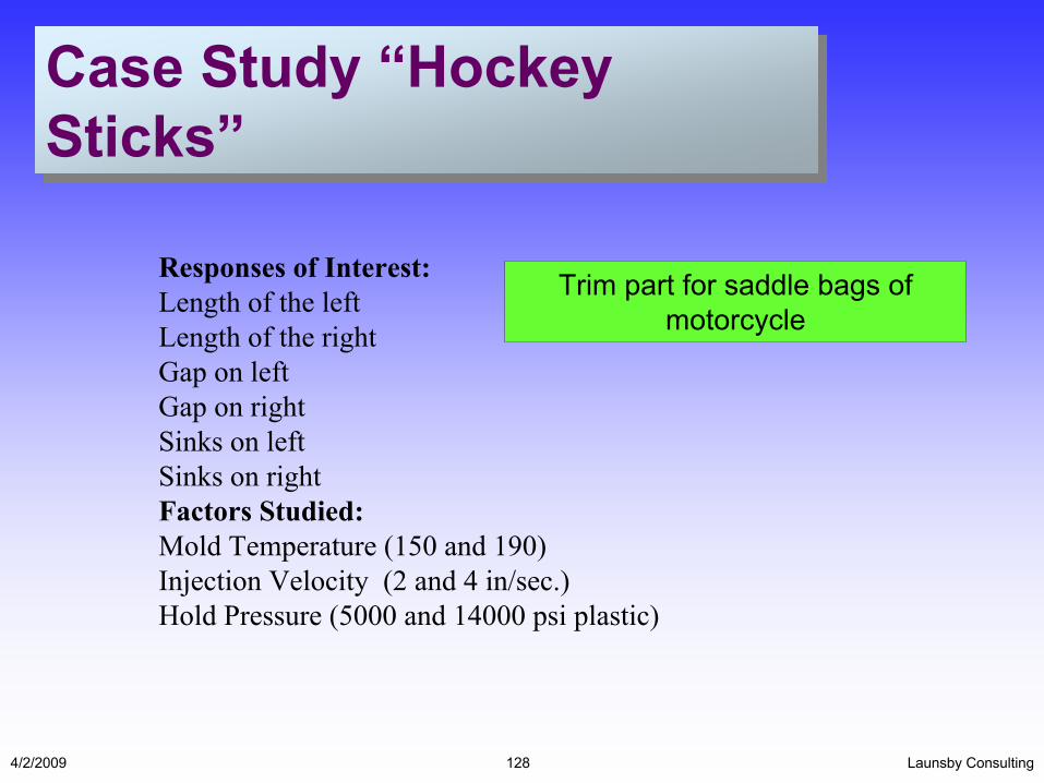
Case Study “Hockey Sticks”Case Study “Hockey Sticks”
Responses of Interest:Length of the leftLength of the rightGap on leftGap on rightSinks on leftSinks on rightFactors Studied:Mold Temperature (150 and 190)Injection Velocity (2 and 4 in/sec.)Hold Pressure (5000 and 14000 psi plastic)
Trim part for saddle bags of motorcycle

Launsby Consulting4/2/2009 129
Case Study (cont.)Case Study (cont.)
Two cavity tool for left and right part

Launsby Consulting4/2/2009 130
Case Study (cont.)Case Study (cont.)
SpeedRelative Visc.
0.5 18,720
1 10,070
1.5 7,225
2 5,715
3 4,270
4 3,540
5 2,950
0.5 1 1.5 2 3 4 5Rel. Visc.
0
5,000
10,000
15,000
20,000
speed
Decided to run DOE at 2 and 4 in/sec

Launsby Consulting4/2/2009 131
Case Study (cont.)Case Study (cont.)
Hold Time Part Weight
2 Less than .088
3 .088
4 .089
5 .089
6 .089
7 .089
A hold time of 6 seconds was selected. Appear to provide ample time for gate seal
Launsby Consulting4/2/2009 132
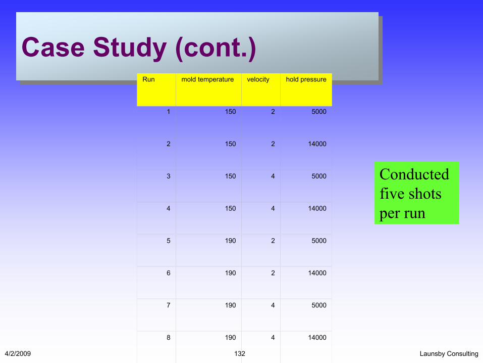
Case Study (cont.)Case Study (cont.)Run mold temperature velocity hold pressure
1 150 2 5000
2 150 2 14000
3 150 4 5000
4 150 4 14000
5 190 2 5000
6 190 2 14000
7 190 4 5000
8 190 4 14000
Conducted five shots per run

Launsby Consulting4/2/2009 133
Case Study (cont.)Case Study (cont.)
-0.8
-0.56
-0.32
-0.08
0.16
0.4
150(-) 190(+)mold temp(A)
2(-) 4(+)velocity(B)
5000(-) 14000(+)hold press(C)
Factors
Main Effects
length right
-0.4
-0.3
-0.2
-0.1
0
0.1
0.2
150(-) 190(+)mold temp(A)
2(-) 4(+)velocity(B)
5000(-) 14000(+)hold press(C)
Factors
Main Effects
length left

Launsby Consulting4/2/2009 134
Case Study (cont.)Case Study (cont.)
2.4
2.6
2.8
3
3.2
3.4
3.6
150(-) 190(+)mold temp(A)
2(-) 4(+)velocity(B)
5000(-) 14000(+)hold press(C)
Factors
Main Effects
gap right
2
2.2
2.4
2.6
2.8
3
3.2
150(-) 190(+)mold temp(A)
2(-) 4(+)velocity(B)
5000(-) 14000(+)hold press(C)
Factors
Main Effects
gap left

Launsby Consulting4/2/2009 135
Case Study (cont.)Case Study (cont.)
1.6
1.8
2
2.2
2.4
2.6
2.8
150(-) 190(+)mold temp(A)
2(-) 4(+)velocity(B)
5000(-) 14000(+)hold press(C)
Factors
Main Effects
sink right
1.8
1.9
2
2.1
2.2
2.3
2.4
150(-) 190(+)mold temp(A)
2(-) 4(+)velocity(B)
5000(-) 14000(+)hold press(C)
Factors
Main Effects
sink left
Student question: does it make sense that these two responses display dramatically different main effects plots for Hold Press?
What could account for this
difference?
Launsby Consulting4/2/2009 136
Case Study (cont.)Case Study (cont.)
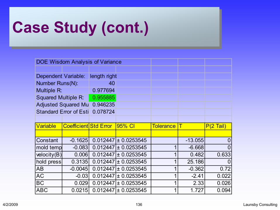
DOE Wisdom Analysis of Variance
Dependent Variable: length rightNumber Runs(N): 40Multiple R: 0.977694Squared Multiple R: 0.955885Adjusted Squared Mu 0.946235Standard Error of Esti 0.078724
Variable Coefficient Std Error 95% CI Tolerance T P(2 Tail)
Constant -0.1625 0.012447 ± 0.0253545 -13.055 0mold temp -0.083 0.012447 ± 0.0253545 1 -6.668 0velocity(B) 0.006 0.012447 ± 0.0253545 1 0.482 0.633hold press( 0.3135 0.012447 ± 0.0253545 1 25.186 0AB -0.0045 0.012447 ± 0.0253545 1 -0.362 0.72AC -0.03 0.012447 ± 0.0253545 1 -2.41 0.022BC 0.029 0.012447 ± 0.0253545 1 2.33 0.026ABC 0.0215 0.012447 ± 0.0253545 1 1.727 0.094
Launsby Consulting4/2/2009 137
Case Study (cont.)Case Study (cont.)
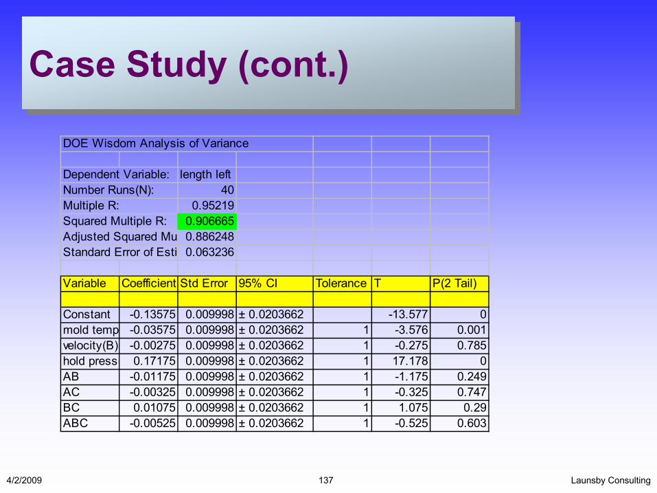
DOE Wisdom Analysis of Variance
Dependent Variable: length leftNumber Runs(N): 40Multiple R: 0.95219Squared Multiple R: 0.906665Adjusted Squared Mu 0.886248Standard Error of Esti 0.063236
Variable Coefficient Std Error 95% CI Tolerance T P(2 Tail)
Constant -0.13575 0.009998 ± 0.0203662 -13.577 0mold temp -0.03575 0.009998 ± 0.0203662 1 -3.576 0.001velocity(B) -0.00275 0.009998 ± 0.0203662 1 -0.275 0.785hold press( 0.17175 0.009998 ± 0.0203662 1 17.178 0AB -0.01175 0.009998 ± 0.0203662 1 -1.175 0.249AC -0.00325 0.009998 ± 0.0203662 1 -0.325 0.747BC 0.01075 0.009998 ± 0.0203662 1 1.075 0.29ABC -0.00525 0.009998 ± 0.0203662 1 -0.525 0.603

Launsby Consulting4/2/2009 138
Case Study (cont.)Case Study (cont.)
DOE Wisdom Analysis of Variance
Dependent Variable: gap rightNumber Runs(N): 40Multiple R: 0.990342Squared Multiple R: 0.980778Adjusted Squared Mu 0.976573Standard Error of Esti 0.085878
Variable Coefficient Std Error 95% CI Tolerance T P(2 Tail)
Constant 2.9575 0.013579 ± 0.0276584 217.808 0mold temp -0.2575 0.013579 ± 0.0276584 1 -18.964 0velocity(B) -0.0225 0.013579 ± 0.0276584 1 -1.657 0.107hold press( 0.4825 0.013579 ± 0.0276584 1 35.534 0AB -0.0175 0.013579 ± 0.0276584 1 -1.289 0.207AC 0.0175 0.013579 ± 0.0276584 1 1.289 0.207BC 0.0225 0.013579 ± 0.0276584 1 1.657 0.107ABC 0.0175 0.013579 ± 0.0276584 1 1.289 0.207
Launsby Consulting4/2/2009 139
Case Study (cont.)Case Study (cont.)
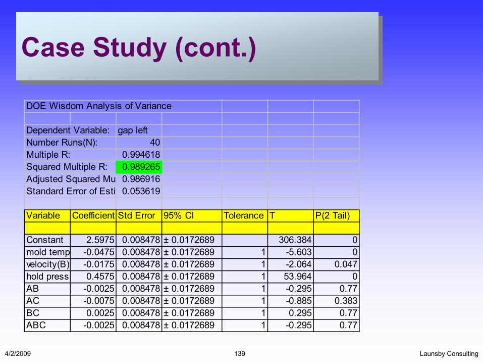
DOE Wisdom Analysis of Variance
Dependent Variable: gap leftNumber Runs(N): 40Multiple R: 0.994618Squared Multiple R: 0.989265Adjusted Squared Mu 0.986916Standard Error of Esti 0.053619
Variable Coefficient Std Error 95% CI Tolerance T P(2 Tail)
Constant 2.5975 0.008478 ± 0.0172689 306.384 0mold temp -0.0475 0.008478 ± 0.0172689 1 -5.603 0velocity(B) -0.0175 0.008478 ± 0.0172689 1 -2.064 0.047hold press( 0.4575 0.008478 ± 0.0172689 1 53.964 0AB -0.0025 0.008478 ± 0.0172689 1 -0.295 0.77AC -0.0075 0.008478 ± 0.0172689 1 -0.885 0.383BC 0.0025 0.008478 ± 0.0172689 1 0.295 0.77ABC -0.0025 0.008478 ± 0.0172689 1 -0.295 0.77

Launsby Consulting4/2/2009 140
Case Study (cont.)Case Study (cont.)
DOE Wisdom Analysis of Variance
Dependent Variable: sink rightNumber Runs(N): 40Multiple R: 0.974639Squared Multiple R: 0.949922Adjusted Squared Mu 0.938967Standard Error of Esti 0.158114
Variable Coefficient Std Error 95% CI Tolerance T P(2 Tail)
Constant 2.275 0.025 ± 0.0509233 91 0mold temp -0.225 0.025 ± 0.050923 1 -9 0velocity(B) 0.225 0.025 ± 0.050923 1 9 0hold press( 0.475 0.025 ± 0.050923 1 19 0AB 0.225 0.025 ± 0.050923 1 9 0AC -0.025 0.025 ± 0.050923 1 -1 0.325BC 0.025 0.025 ± 0.050923 1 1 0.325ABC 0.025 0.025 ± 0.050923 1 1 0.325

Launsby Consulting4/2/2009 141
Case Study (cont.)Case Study (cont.)
DOE Wisdom Analysis of Variance
Dependent Variable: sink leftNumber Runs(N): 40Multiple R: 0.725476Squared Multiple R: 0.526316Adjusted Squared Mu 0.422697Standard Error of Esti 0.33541
Variable Coefficient Std Error 95% CI Tolerance T P(2 Tail)
Constant 2.1 0.053033 ± 0.108025 39.598 0mold temp -0.15 0.053033 ± 0.108025 1 -2.828 0.008velocity(B) 0.05 0.053033 ± 0.108025 1 0.943 0.353hold press( 0 0.053033 ± 0.108025 1 0 1AB -0.2 0.053033 ± 0.108025 1 -3.771 0.001AC 0.15 0.053033 ± 0.108025 1 2.828 0.008BC -0.05 0.053033 ± 0.108025 1 -0.943 0.353ABC 0.1 0.053033 ± 0.108025 1 1.886 0.068

Launsby Consulting4/2/2009 142
Case Study (cont.)Case Study (cont.)
-6
-4
-2
0
2
4
6
1 2 3 4 5 6 7 8 9 10111213141516171819202122232425262728293031323334353637383940Run Order
left Studentized Resid
Residual Scatter Plot

Launsby Consulting4/2/2009 143
Case Study (cont.)Case Study (cont.)
D(composite)
mold temp
hold press
Response Surface**velocity(B)=2.00000
150
158
166
174
182
190
50006800
860010400
1220014000
0
0.2
0.4
0.6
0.8
1
Launsby Consulting4/2/2009 144
Case Study Best Set PointsCase Study Best Set Points
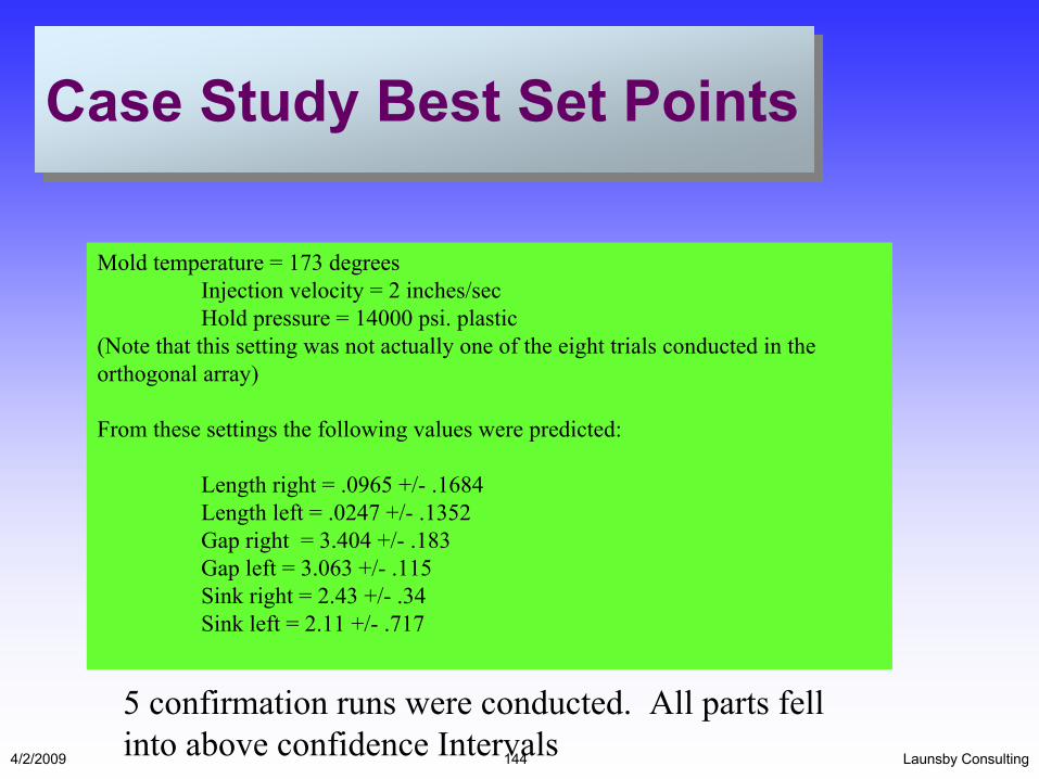
Mold temperature = 173 degreesInjection velocity = 2 inches/secHold pressure = 14000 psi. plastic
(Note that this setting was not actually one of the eight trials conducted in the orthogonal array)
From these settings the following values were predicted:
Length right = .0965 +/- .1684Length left = .0247 +/- .1352Gap right = 3.404 +/- .183Gap left = 3.063 +/- .115Sink right = 2.43 +/- .34Sink left = 2.11 +/- .717
5 confirmation runs were conducted. All parts fell into above confidence Intervals
Launsby Consulting4/2/2009 145
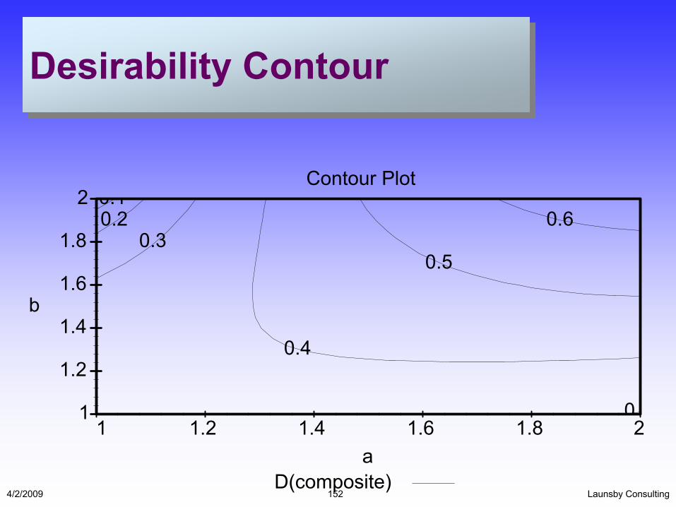
Desirability FunctionsDesirability Functions
• What are They?• Why are They Needed?• What are the Steps Required?
– For Each Response, Determine a Shape– For Each Response, Determine an Importance
Weight– Analyze Composite D
• What are They?• Why are They Needed?• What are the Steps Required?
– For Each Response, Determine a Shape– For Each Response, Determine an Importance
Weight– Analyze Composite D

Launsby Consulting4/2/2009 146
Composite D ExampleComposite D Example
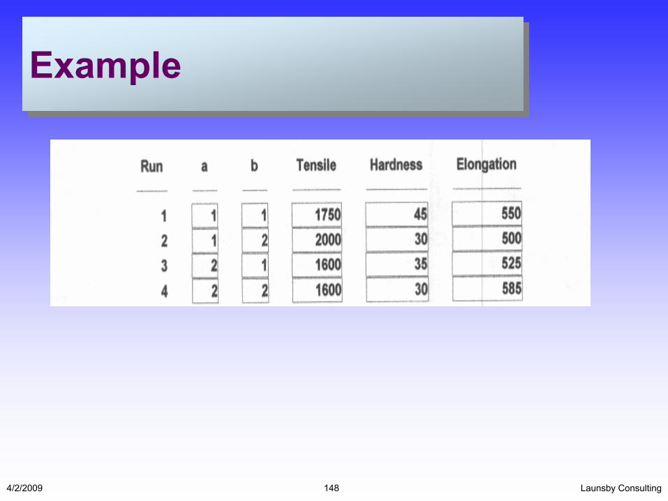
FACTOR LOW HIGH
A 1 2
B 1 2
Launsby Consulting4/2/2009 147
Composite D ExampleComposite D Example
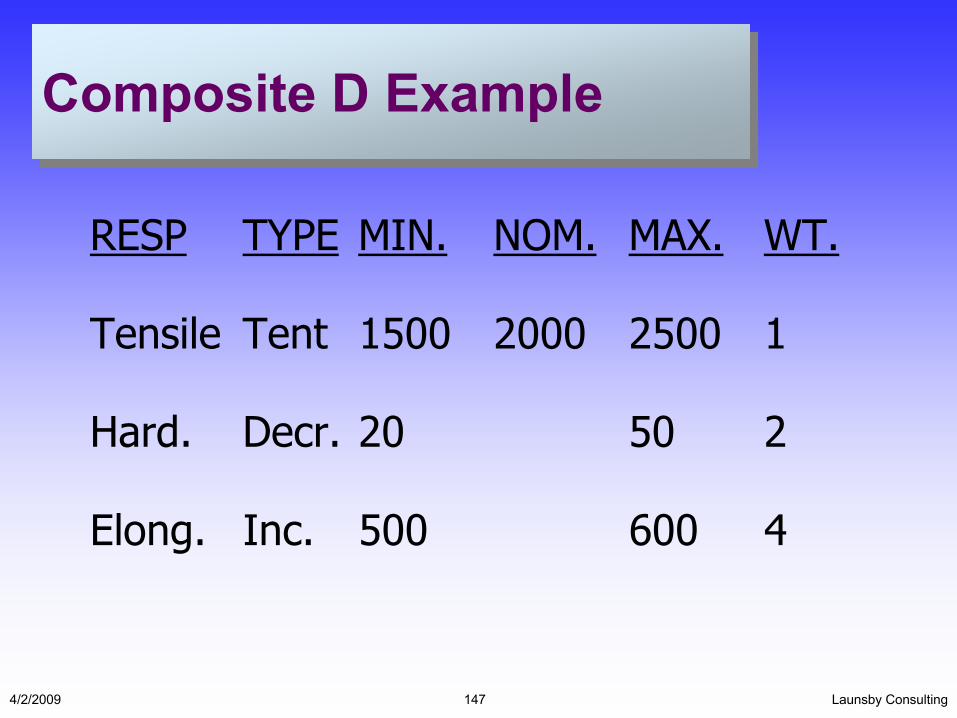
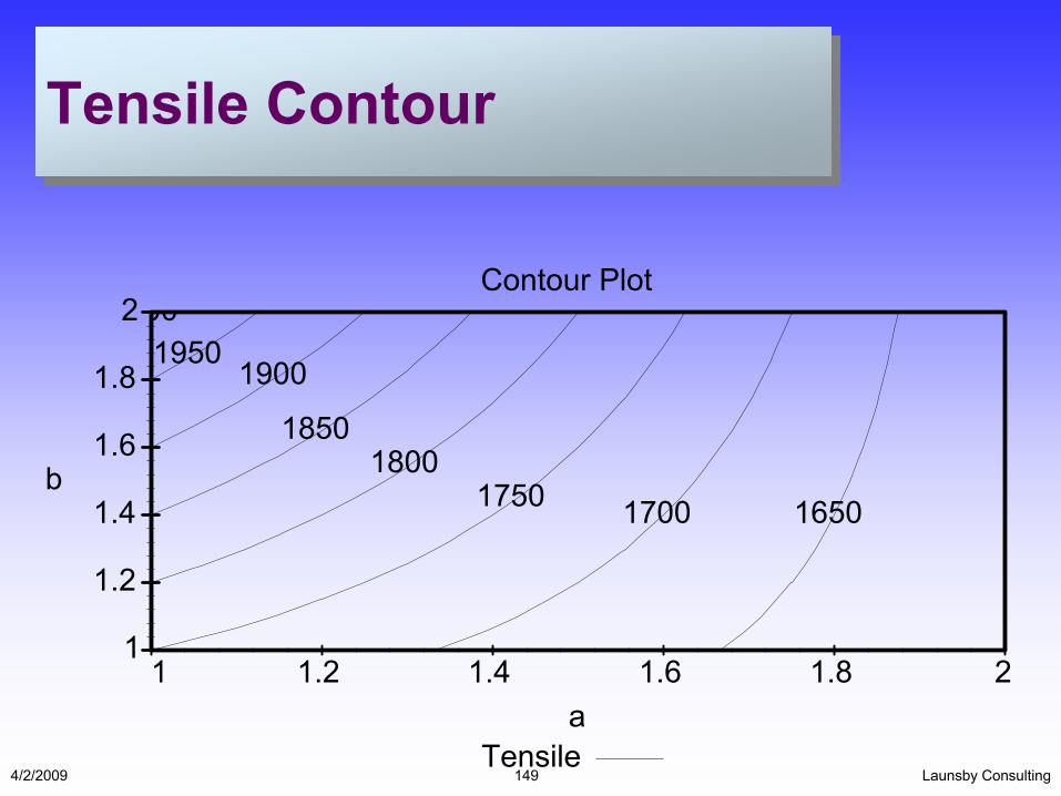
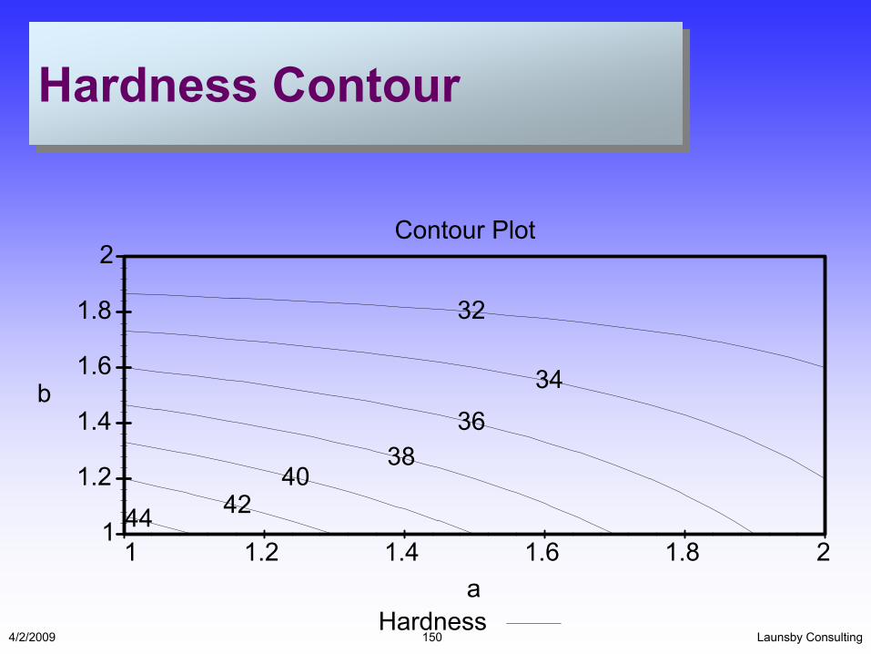
RESP TYPE MIN. NOM. MAX. WT.
Tensile Tent 1500 2000 2500 1
Hard. Decr. 20 50 2
Elong. Inc. 500 600 4
Launsby Consulting4/2/2009 148
ExampleExample
Launsby Consulting4/2/2009 149
Tensile ContourTensile Contour
1 1.2 1.4 1.6 1.8 2a
1
1.2
1.4
1.6
1.8
2
b
Contour Plot
Tensile
1750 17001800
1850
19001950
00
1650
Launsby Consulting4/2/2009 150
Hardness ContourHardness Contour
1 1.2 1.4 1.6 1.8 2a
1
1.2
1.4
1.6
1.8
2
b
Contour Plot
Hardness
44 4240
3836
34
32

Launsby Consulting4/2/2009 151
Elongation ContourElongation Contour
1 1.2 1.4 1.6 1.8 2a
1
1.2
1.4
1.6
1.8
2
b
Contour Plot
Elongation
540530
540550
560570
580
530
520510
Launsby Consulting4/2/2009 152
Desirability ContourDesirability Contour
1 1.2 1.4 1.6 1.8 2a
1
1.2
1.4
1.6
1.8
2
b
Contour Plot
D(composite)
0.30.20.1
0.4
0.5
0.6
0

Launsby Consulting4/2/2009 153
SummarySummary
• Understand the Technology of Molding
• Use the Four Plastic Variables as the Foundation for DOE
• Physics First
• 510 Rule
• Understand the Technology of Molding
• Use the Four Plastic Variables as the Foundation for DOE
• Physics First
• 510 Rule