Powder Technology, 71 (1992) 87-99 87

Experimental and theoretical porosity profiles in a two-dimensional gas-fluidized bed with a central jet

J. A. M. Kuipers, H. Tammes, W. Prins and W. P. M. van Swaaij Department of Chemical Engineering, Twente University of Technology, P.O. Box 217, 7500 AE Enschede, (Netherlands)

(Received October 18, 1990; in revised form November 26, 1991)

Abstract

A light transmission technique has been developed for measurement of the local porosity in two-dimensional gas-fluidized beds. The principles of liquid-solid fluidization and vibrofluidization were employed to perform the necessary calibration. Time-averaged porosity profiles have been measured in a thin two-dimensional gas-fluidized bed with a central rectangular jet. These profiles were predicted satisfactorily with a previously developed first principles hydrodynamic model, without the use of any fitted parameters. The hydrodynamic model is based on a two-fluid model approach in which both phases are considered to be continuous and fully interpenetrating.

Introduction

It is well-known that the porosity or bed voidage E is a key factor in characterizing the hydrodynamics and the heat and mass transfer properties of gas-fluidized beds. A number of different experimental techniques have been developed for measurement of the bed voidage distribution in gas-fluidized beds. Pressure drop measurements [l], capacitance probes [2, 31, as well as X-ray [4] and y-ray [5-111 absorption and light transmission [12-141 techniques have all been employed.

Gidaspow et al. have argued [lo] that disturbance of the internal flow behaviour of the bed may occur when probe techniques (for example: capacitance and light probes) are employed for these measurements. X-ray and -y-ray transmission techniques do not suffer from this disadvantage: usually both the emittor and detector are positioned outside the bed. Because 3/- rays penetrate through steel, y-ray attenuation tech- niques are often preferred, especially for high pressure fluidization studies.

Despite certain practical limitations, the above ex- perimental techniques have provided valuable infor- mation on density patterns in gas-fluidized beds and the effect of gas distributor design upon these density patterns. However, through recent advances in the field of computational fluid dynamics and computer tech- nology, theoretical prediction of the hydrodynamics of gas-fluidized beds (bubble formation, bed voidage pro- files, gas and solids motion) from first principles should become feasible in the near future. This possibility will

offer an attractive alternative approach to obtain density patterns and other hydrodynamic characteristics of gas- fluidized beds, especially in those cases where the use of experimental methods is severely restricted by tech- nical and/or financial constraints.

Present theoretical models of gas-fluidized beds are still lacking full experimental validation which implies that they cannot yet be considered as reliable design tools for complex fluidized systems. In order to validate these theoretical models experimentally, two-dimen- sional gas-fluidized beds play an important role because of the possibility of visual observation of the bed behaviour. Such a two-dimensional gas-fluidized bed has also been used in the present investigation. The first successful computational approach to calculate the instantaneous and time-averaged porosity distributions in a two-dimensional gas-fluidized bed with a central jet, from the basic hydrodynamic equations of change, was made by Gidaspow and Ettehadieh [15]. Their two- dimensional fluid bed construction represented roughly a cross-section of the Westinghouse gasifier [16, 171. The calculated porosity distributions agreed satisfac- torily with distributions obtained experimentally by -y- ray densitometry. Bouillard et al. [ll, 181 extended this theoretical and experimental work by studying fluidi- zation in a two-dimensional b.ed provided with an immersed rectangular obstacle which represented a horizontal heat exchanger tube. Satisfactory agreement was reported between the theoretical predictions and the experimental data. The principal differences be- tween theory and experiment were attributed to asym- metries present in the experiment and to the simplified

0032-5910/92/$5.00 0 1992 - Elsevier Sequoia. All rights reserved

88

solids rheology their hydrodynamic model.

The main objective study is to provide first

ciples hydrodynamic model of gas-fluidized beds [19] by comparing theoretically calculated time-averaged porosity profiles for a two-dimensional gas-fluidized bed with a central jet with the corresponding experimental data. Kuipers et al. [20] have already demonstrated that the hydrodynamic model can predict bubble sizes in a two-dimensional gas-fluidized bed satisfactorily, without the use of any fitted parameters.

Experimental

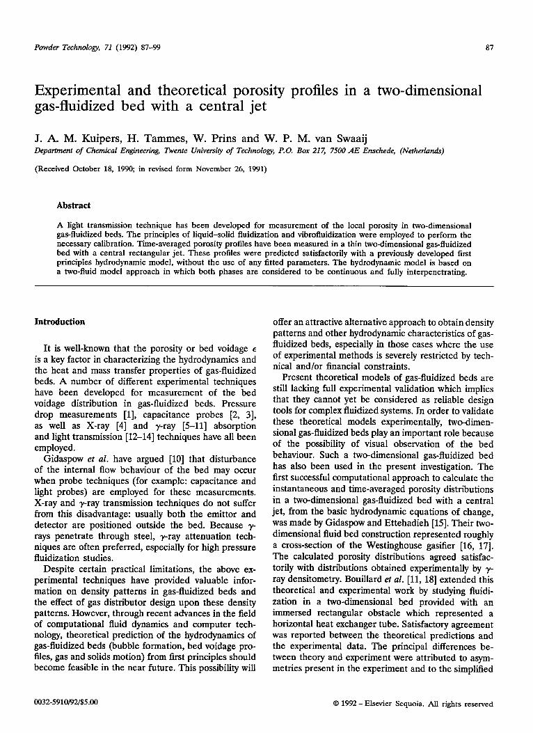
Equipment and experimental procedure The experiments were carried out in the thin two-

dimensional gas-fluidized bed described in our previous paper [20]. Figure 1 shows a schematic representation of the experimental set-up used for the porosity mea- surements. It consists of a fluidized bed section made of 0.015 m thick glass plates and a gas distributor section made of 0.015 m thick transparent Plexiglass plates. To approximate true two-dimensional behaviour [21] and to reduce any severe restriction of solids flow by the ‘wall effect’, the bed thickness (distance between the front and back plate) was chosen to be 0.015 m. A porous plate fitted with a central rectangular pipe (internal dimensions 15.0 mm X 15.0 mm) was used to introduce humidified air which served as the fluidizing medium. To eliminate three-dimensional entrance ef- fects near the orifice region it was decided to use a rectangular instead of a circular orifice pipe [lo]. Both the mass flow rate of the fluidizing air injected through

- flange

_ suppon rack for optical sensor

Y

t

x

the porous plate, and the mass flow rate of the additional air injected through the central pipe were controlled independently by calibrated thermal mass flow con- trollers.

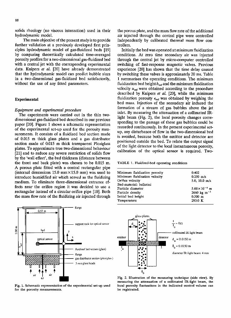
Initially the bed was operated at minimum fluidization conditions. At zero time secondary air was injected through the central jet by micro-computer controlled switching of fast-response magnetic valves. Previous experience [20] has shown that the time delay caused by switching these valves is approximately 20 ms. Table 1 summarises the operating conditions. The minimum fluidization bed height /z,,,~ and the minimum fluidization velocity u,r were obtained according to the procedure described by Kuipers et al. [20], while the minimum fluidization porosity E,.,,~ was obtained by weighing the bed mass. Injection of the secondary air induced the formation of a stream of gas bubbles above the jet inlet. By measuring the attenuation of a collimated IR- light beam (Fig. 2), the local porosity changes corre- sponding to the passage of these gas bubbles could be recorded continuously. In the present experimental set- up, any disturbance of flow in the two-dimensional bed is avoided, because both the emittor and detector are positioned outside the bed. To relate the output signal of the light detector to the local instantaneous porosity, calibration of the optical sensor is required. Two-

TABLE 1. Fluidized-bed operating conditions

Minimum fluidization porosity Minimum fluidization velocity Orifice velocity Bed-material: ballotini Particle diameter Particle density Initial bed height Temperature

0.402 0.250 m/s 5.0, 10.0 m/s

5.00X lo+ m 2660 kg mm3 0.500 m 293.0 K

- fluidized bed section (glass)

- flange - gas distributor section (plexiglass)

- 3 mm glass beads

I Fig. 1. Schematic representation of the experimental set-up used for the porosity measurements.

glass plates

f = f(E) 0

collimated IR-light beam

dw=0.0150m

6, = 0.0150 m

diameter [R-light beam: 4

Fig. 2. Illustration of the measuring technique (side view). By measuring the attenuation of a collimated IR-light beam, the local porosity fluctuations in the indicated control volume can be registrated.

a9

dimensional porosity profiles can be constructed from measurements at different locations.

Optical sensor A powerful lensed IR-LED (Dolan and Jenner, model

7051-06) was used to generate the collimated IR-light beam. The IR-LED was connected to an adjustable power supply (Delta Elektronica, model E015-2). An optical waveform analyzer (Photodyne, model 1500 XP) converts the optical signal into an electrical output signal. This instrument combines important features such as high sensitivity, fast response and good op- erational stability. A fibre optic cable (Dolan and Jenner, type B-836) guided the light from the detection point to the actual light detector.

Data acqukition and analysis An IBM compatible micro-computer was used to

facilitate data acquisition and data analysis. To increase the resolution for the low-porosity region (packed bed conditions) the electrical output of the optical waveform analyzer was fed to a logarithmic amplifier (Analog Devices, model 759N). The amplified output signal was converted into digital data via a 1Zbit AD-converter (Analog Devices, model RTI815-FA) connected into an expansion slot of the micro-computer. High frequency sampling was achieved by storing the data in a DMA buffer. A PASCAL computer program has been de- veloped for the postprocessing of the accumulated data.

Calibration A crucial aspect in the measurements is the nec-

essary calibration of the optical sensor. At present, optical theory does not provide a sound theoretical basis to relate quantitatively the recorded light trans- mission to the particle volume fraction in the control volume under consideration, which necessitates exper- imental calibration of the optical sensor. The principal difficulty to be overcome here is the realization of a homogeneous (i.e., with no gas bubbles present) gas- fluidized bed of solid particles of a specified particle volume fraction, while making the light transmission measurements. At the same time it should be possible to vary this particle volume fraction over a wide range to produce a calibration curve for the light transmission as a function of bed porosity. The difficulty can be understood by recalling the heterogeneous character of gas-solid fluidization. The present system of air- fluidized ballotini with an average particle diameter of 500 pm and a true density of 2 660 kg mw3, falls within the B-category according to Geldart’s classification [22]. Type B-fluidization has no regime of homogeneous bed expansion. As shown below, the calibration problem has been solved by employing liquid-solid fluidization and vibrofluidization.

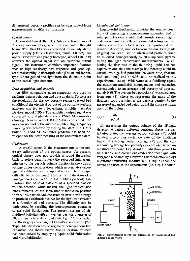
Liquid-solid fluidization Liquid-solid fluidization provides the unique possi-

bility of generating a homogeneous expanded bed of solid particles over a wide bed porosity range. Figure 3 shows schematically the experimental set-up used for calibration of the optical sensor by liquid-solid flui- dization. A second, smaller two-dimensional bed (made of glass) has been used in which solid particles could be fluidized homogeneously by 50% aqueous glycerol during the light transmission measurements. By ad- justing the flow rate of the fluidizing liquid, the bed expansion and thus the average bed porosity could be varied. Average bed porosities between E= ep (packed bed conditions) and E = 0.95 could be realized in this experimental set-up. With water as a fluidizing agent, the maximum attainable homogeneous bed expansion corresponded to an average bed porosity of approxi- mately 0.80. The average bed porosity (E) was calculated from eqn. (l), where m, represents the mass of the fluidized solid particles, ps the particle density, h, the measured expanded bed height andA the cross-sectional area of the column.

(e)=l- m, PshJ (1)

By measuring the output voltage of the IR-light detector at various different positions above the dis- tributor plate, the average output voltage (V) could be determined. For each flow rate of the fluidizing liquid, this average output voltage (V) and the cor- responding average bed porosity (E) were used to obtain a calibration point. Liquid-solid fluidization proved to be a simple and convenient calibration technique with very good repeatability. However, this technique employs a different fluidizing medium (i.e. a liquid) than the actual one used in the experiments (i.e. air). Undoubt-

t @“.I n glass ’

dw=0.0150m

power supply

- y.. -

Fig. 3. Experimental set-up for calibration by liquid-solid flui- dization (side view).

90

edly, the absorption and reflection characteristics of the IR-light in the air-solid system and the liquid-solid system are generally not identical. The difference in optical behaviour between gas-solid and liquid-solid systems has also been noted by Hartge et al. [23]. Calibration by applying liquid-solid fluidization is only possible when the effect of these differences can be eliminated. This has been investigated by comparison of the liquid-solid calibration method with another one, viz. calibration in a cell containing air and solid particles ‘fluidized’ homogeneously by vibration. This latter cal- ibration method, termed ‘vibrofluidization’, has also been applied by Yang et al. [14] for the calibration of their light probe.

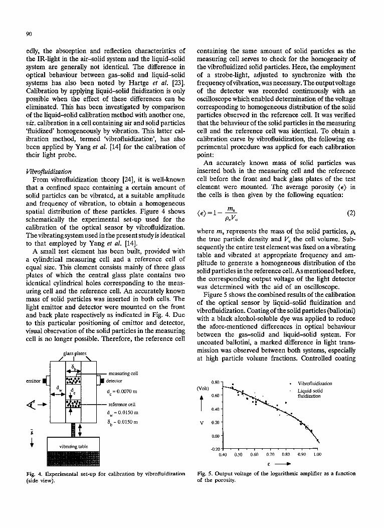
Vibrofuidization From vibrofluidization theory [24], it is well-known

that a confined space containing a certain amount of solid particles can be vibrated, at a suitable amplitude and frequency of vibration, to obtain a homogeneous spatial distribution of these particles. Figure 4 shows schematically the experimental set-up used for the calibration of the optical sensor by vibrofluidization. The vibrating system used in the present study is identical to that employed by Yang et al. [14].

A small test element has been built, provided with a cylindrical measuring cell and a reference cell of equal size. This element consists mainly of three glass plates of which the central glass plate contains two identical cylindrical holes corresponding to the meas- uring cell and the reference cell. An accurately known mass of solid particles was inserted in both cells. The light emittor and detector were mounted on the front and back plate respectively as indicated in Fig. 4. Due to this particular positioning of emittor and detector, visual observation of the solid particles in the measuring cell is no longer possible. Therefore, the reference cell

glass plates

emittor

<-

* I vibrating table

Fig. 4. Experimental set-up for calibration by vibrofluidization (side view).

containing the same amount of solid particles as the measuring cell serves to check for the homogeneity of the vibrofluidized solid particles. Here, the employment of a strobe-light, adjusted to synchronize with the frequency ofvibration, was necessary. The output voltage of the detector was recorded continuously with an oscilloscope which enabled determination of the voltage corresponding to homogeneous distribution of the solid particles observed in the reference cell. It was verified that the behaviour of the solid particles in the measuring cell and the reference cell was identical. To obtain a calibration curve by vibrofluidization, the following ex- perimental procedure was applied for each calibration point:

An accurately known mass of solid particles was inserted both in the measuring cell and the reference cell before the front and back glass plates of the test element were mounted. The average porosity (E) in the cells is then given by the following equation:

(e)=l- m, PSVC

where m, represents the mass of the solid particles, ps the true particle density and V, the cell volume. Sub- sequently the entire test element was fixed on a vibrating table and vibrated at appropriate frequency and am- plitude to generate a homogeneous distribution of the solid particles in the reference cell. As mentioned before, the corresponding output voltage of the light detector was determined with the aid of an oscilloscope.

Figure 5 shows the combined results of the calibration of the optical sensor by liquid-solid fluidization and vibrofluidization. Coating of the solid particles (ballotini) with a black alcohol-soluble dye was applied to reduce the afore-mentioned differences in optical behaviour between the gas-solid and liquid-solid system. For uncoated ballotini, a marked difference in light trans- mission was observed between both systems, especially at high particle volume fractions. Controlled coating

0.80 - . l Vibrofluidization (Volt) Liquid-solid

t

fluidization

0.40 -

0.00 -

-0.20 . 1 . I - I . I . b . I 0.40 0.50 0.60 0.70 0.80 0.90 1 .oo

Ed

Fig. 5. Output voltage of the logarithmic amplifier as a function of the porosity.

91

of the solid particles could be achieved, in a small 15- cm diameter gas-fluidized bed. The progress of this process was monitored by constant withdrawal of small samples of solid particles from the bed, and subsequent comparison of the light transmission in the gas-solid and liquid-solid system. When the difference in the light transmission 2rs. porosity curves between the gas-solid system (i.e. the vibro-fluidized bed) and the liquid-solid system (i.e. the (small) liquid-fluidized bed) had become negligible, the coating process was con- sidered to be complete. The requirement of negligible difference in light transmission over the entire porosity range (0.40 < ~<0.95) implies that the amount of dye did not depend on the porosity. In the experiments, the bed-material consisted of coated ballotini.

Both calibration techniques (i.e. liquid-solid fluidi- zation and vibrofluidization) can, in fact, be viewed as complementary. Liquid-solid fluidization provides the possibility of producing a calibration curve with a simple and convenient technique but employs a different flui- dizing agent than the one used in the experiments. The effect of the fluidizing agent on the calibration can subsequently be determined by comparison with that obtained by vibrofluidization.

Hydrodynamic model

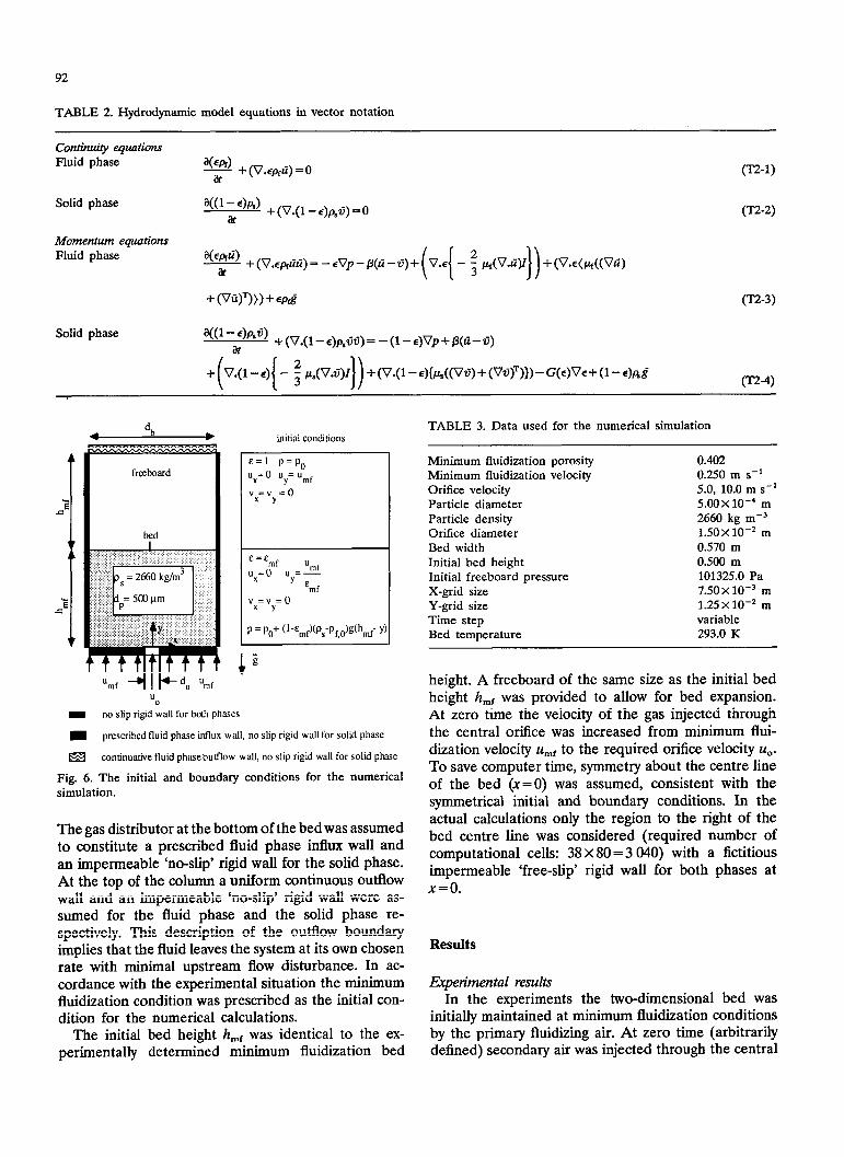
The previously developed theoretical model of gas- fluidized beds [19] is based on a two-fluid model ap- proach in which both phases are considered to be continuous and fully interpenetrating. In fact, the equa- tions used in the theoretical model can be seen as a generalization of the Navier-Stokes equations for two interacting continua. Previous work [20] has shown that the hydrodynamic model predicts experimentally ob- served bubble diameters in two-dimensional gas-flui- dized beds satisfactorily without the use of fitted pa- rameters. The model employs two sets of conservation equations, governing the balance of mass, momentum and thermal energy in each phase. Table 2 shows the mass and momentum conservation equations for both phases in vector form. In the present study, fluidization in an isothermal gas-fluidized bed will be considered: the solution of the thermal energy equations is not required here. Due to the mathematical complexity of the equations of change a numerical solution method, described elsewhere [25] has been adopted. The nu- merical technique has been embodied in an unsteady two-dimensional computer code written in VAX-PAS- CAL.

The computer model calculates the porosity, pressure, the fluid and solid phase temperatures if required, and the velocity fields of both phases in two-dimensional Cartesian or (axi-symmetrical) cylindrical coordinates.

These variables constitute the so called “primary” or basic variables. For closure of the set of balance equa- tions, specification of the constitutive relations is re- quired which implies specification of all other variables in terms of the basic variables. Incorporation of these constitutive equations introduces the necessary empir- ical information in the present theoretical model of gas-fluidized beds.

Constitutive equations - Fluid phase density pf and solid phase density pS.

The fluid phase density is related to the pressure and fluid phase temperature by the ideal gas law. For the solid phase microscopic incompressibility was assumed; accordingly a specified constant density was taken.

- Interphase momentum transfer coefficient /?. For porosities E < 0.80 the interphase momentum trans- fer coefficient has been obtained from the well-known vectorial Ergun equation whereas for porosities E> 0.80 the interphase momentum transfer coefficient has been derived from the correlation of Wen and Yu (Kuipers et al. [19, 201 and Kuipers [25]).

- Fluid phase shear viscosity PI and solid phase shear viscosity Pi. For the fluid phase shear viscosity pf the corresponding microscopic shear viscosity of the fluidizing medium (air at approximately atmospheric conditions (p = 101.3 kPa, T=293 K)) has been used (pf=2.0x lo-’ Pa s). Apparent bed viscosities, for spherical ballotini with a narrow particle size distribution, have been determined experimentally by Schtigerl et al. [26] and empirically by Grace [27]. Based on the results obtained by Schiigerl and Grace the solid phase shear viscosity pL, has been taken as 1.0 Pa s.

- Solid phase elastic modulus G(E). As discussed in the previous paper [19], the solid phase elastic modulus G(E) is important from both a physical and a numerical viewpoint and has been incorporated in the model according to the following generalized form:

G(E) = - G,{exp(c(e* - E))} (3)

where G, represents the normalizing units factor, c the compaction modulus and E* the compaction gas phase volume fraction. To prevent unacceptable bed com- paction G, has been taken as 1 Pa, with c= 100 and l *=o45 . .

Numerical simulation Figure 6 shows the initial and boundary conditions

used for the numerical simulation; the corresponding numerical data are presented in Table 3. Two-dimen- sional Cartesian coordinates were used in the com- putations. The left and right side walls were modelled as impermeable, ‘no-slip’ rigid walls for both phases.

92

TABLE 2. Hydrodynamic model equations in vector notation

Continuity equations Fluid phase

Solid phase

Momentum equations Fluid phase

a+,) T + (V.e&) = 0

a((1 - ~)h) at

+(V.(1-c)pbC)=O

U-2-1)

U-2-2)

Cl.23)

Solid phase a((1 - E)f%?J) +(V.(l-•)p,G)= -(l-c)vp+p(li-ti)

+(V.(l -c){k((Vti) +(Vti)=)})-G(e)Ve+(l -r)~g W-4)

freeboard

initial conditions

ux=o uy= ” ml vx=v =o

Y

E=E ml ”

ux= 0 “Y=f E

mf

vx=v =o Y

p = po+ (l-y,,f)(p,-pf ,,Mh,,,i Y:

no slip rigid wall for both phases

prescribed fluid phase intlux wall, no slip rigid wall for solid phase

Fig. 6. simulation.

continuative fluid phaseoutflow wall, no slip rigid wall for solid phase

The initial and boundary conditions for the numerical

The gas distributor at the bottom of the bed was assumed to constitute a prescribed fluid phase influx wall and an impermeable ‘no-slip’ rigid wall for the solid phase. At the top of the column a uniform continuous outflow wall and an impermeable ‘no-slip’ rigid wall were as- sumed for the fluid phase and the solid phase re- spectively. This description of the outflow boundary implies that the fluid leaves the system at its own chosen rate with minimal upstream flow disturbance. In ac- cordance with the experimental situation the minimum fluidization condition was prescribed as the initial con- dition for the numerical calculations.

The initial bed height h,f was identical to the ex- perimentally determined minimum fluidization bed

TABLE 3. Data used for the numerical simulation

Minimum fluidization porosity 0.402 Minimum fluidization velocity 0.250 m s-l Orifice velocity 5.0, 10.0 m s-l Particle diameter 5.00 X 10m4 m Particle density 2660 kg mm3 Orifice diameter 1.50X lo-* m Bed width 0.570 m Initial bed height 0.500 m Initial freeboard pressure 101325.0 Pa X-grid size 7.50 X lo-’ m Y-grid size 1.25 X lo-* m Time step variable Bed temperature 293.0 K

height. A freeboard of the same size as the initial bed height hmt was provided to allow for bed expansion. At zero time the velocity of the gas injected through the central orifice was increased from minimum flui- dization velocity u,.,,~ to the required orifice velocity u,. To save computer time, symmetry about the centre line of the bed (x=0) was assumed, consistent with the symmetrical initial and boundary conditions. In the actual calculations only the region to the right of the bed centre line was considered (required number of computational cells: 38 X 80 = 3 040) with a fictitious impermeable ‘free-slip’ rigid wail for both phases at x=0.

Results

Experimental results In the experiments the two-dimensional bed was

initially maintained at minimum fluidization conditions by the primary fluidizing air. At zero time (arbitrarily defined) secondary air was injected through the central

93

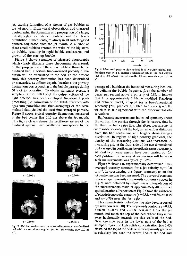
jet, causing formation of a stream of gas bubbles at the jet mouth. From visual observations and triggered photographs, the formation and propagation of a large, initially cylindrical start-up bubble could be clearly established. Subsequently, relatively small and elongated bubbles originated from the jet mouth. A number of these small bubbles entered the wake of the big start- up bubble, resulting in rapid bubble coalescence and growth of the start-up bubble.

Figure 7 shows a number of triggered photographs which clearly illustrate these phenomena. As a result of the propagation of these gas bubbles through the fluidized bed, a certain time-averaged porosity distri- bution will be established in the bed. In the present study this porosity distribution has been determined by measuring, at different spatial locations, the porosity fluctuations corresponding to the bubble passage during 60 s of jet operation. To obtain stationary results, a sampling rate of 500 Hz of the output voltage of the light detector has been employed. Subsequent post- processing (i.e. conversion of the 30 000 recorded volt- ages into porosities and time-averaging) of the accu- mulated data yielded the local time-averaged porosity. Figure 8 shows typical porosity fluctuations measured at the bed centre line 3.13 cm above the jet mouth. This figure clearly shows the oscillatory nature of the fluidized system. Each oscillation corresponds to the

t = 0.300 s t = 0.340 s

t = 0.360 s t = 0.400 s

Fig. 7. Bubble coalescence in a two-dimensional gas-fluidized bed with a central rectangular jet. Jet air velocity u,= 10.0 m S-l.

1.00

t

0.90

0.80

E 0.70

0.60

0.50

0.40

0.30 : * I 1 I . I . I 1 1

0.00 0.40 0.80 1.20 1.60 2.00

t d (S)

Fig. 8. Measured porosity fluctuations in a two-dimensional gas- fluidized bed with a central rectangular jet, at the bed centre line 3.13 cm above the jet mouth. Jet air velocity u,=lO.O m s-‘.

passage of a bubble at the indicated measuring location. By defining the bubble frequency fb as the number of peaks per second above a porosity of 0.85, it follows that f, is approximately 6 Hz. A modified Davidson and Schiiler model, adapted for a two-dimensional geometry [20], predicts a bubble frequency fb =5 Hz which is in fair agreement with the experimental ob- servations.

Exploratory measurements indicated symmetry about the vertical line passing through the jet centre, that is, the fluidized bed centre line. Therefore, measurements were made for only half the bed, viz. at various distances from the bed centre line and heights above the gas distributor. In regions of high porosity gradients, the density of the measuring locations was increased. A measuring grid at the front side of the two-dimensional bed was used in positioning the optical sensor accurately. At least two measurements have been carried out for each position: the average deviation in result between such measurements was typically l-2%.

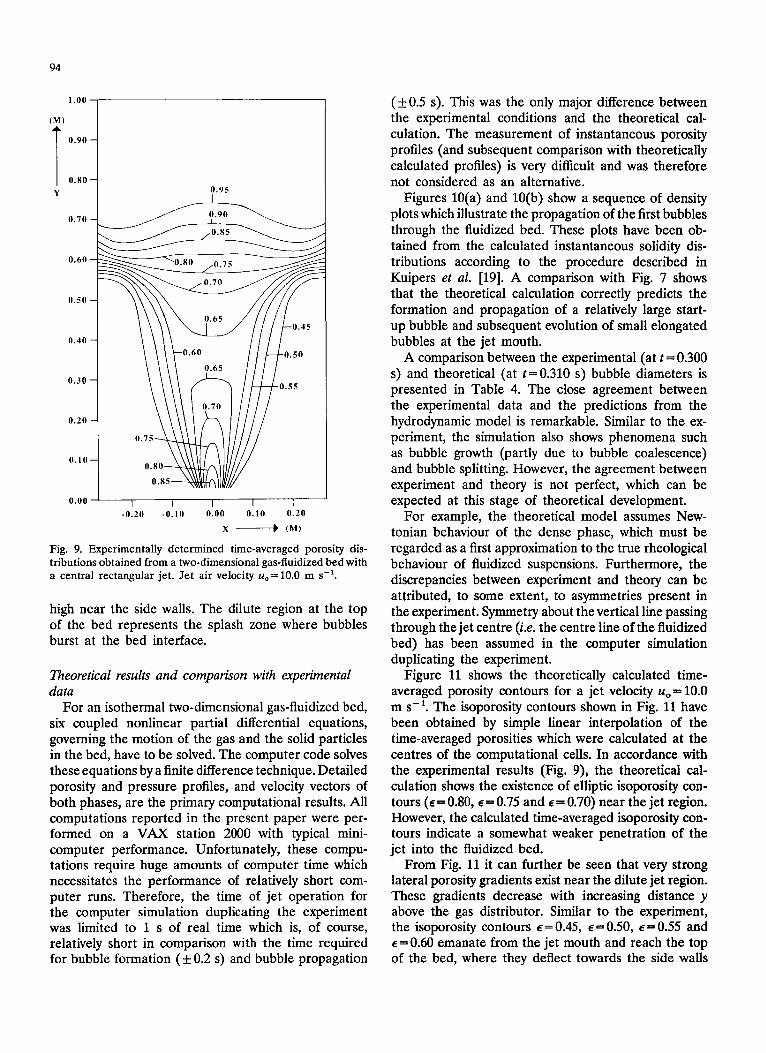
Figure 9 shows the experimentally determined time- averaged porosity contours for a jet velocity uO= 10.0 m s-l. In constructing this figure, symmetry about the jet centre line has been assumed. The curves of constant time-averaged porosity (isoporosity contours), shown in Fig. 9, were obtained by simple linear interpolation of the measurements made at approximately 400 distinct spatial locations. Inspection of Fig. 9 shows the existence of elliptic isoporosity contours (e = 0.85, E= 0.80, E= 0.75 and l =0.70) near the jet region.

This characteristic behaviour has also been reported by Gidaspow et al. [lo]. The isoporosity contours E = 0.45, l =0.50, g=0.55 and E= 0.60 originate from the jet mouth and reach the top of the bed, where they curve away horizontally towards the side walls of the bed. Near the side walls in the lower part of the bed a slumped region of high solids concentration (EF 0.40) exists. At the top of the bed the vertical porosity gradient is relatively low near the centre line of the bed and

94

1.00

(Ml

T

0.90

0.80

Y

0.70

0.60

0.50

0.40

0.30

0.20

0.10

0.00

\ \

b -

I-

I I I I I -0.20 -0.10 0.00 0.10 0.20

X + CM)

Fig. 9. Experimentally determined time-averaged porosity dis- tributions obtained from a two-dimensional gas-fluidized bed with a central rectangular jet. Jet air velocity u,= 10.0 m s-‘.

high near the side walls. The dilute region at the top of the bed represents the splash zone where bubbles burst at the bed interface.

Theoretical results and comparison with experimental data

For an isothermal two-dimensional gas-fluidized bed, six coupled nonlinear partial differential equations, governing the motion of the gas and the solid particles in the bed, have to be solved. The computer code solves these equations by a finite difference technique. Detailed porosity and pressure profiles, and velocity vectors of both phases, are the primary computational results. All computations reported in the present paper were per- formed on a VAX station 2000 with typical mini- computer performance. Unfortunately, these compu- tations require huge amounts of computer time which necessitates the performance of relatively short com- puter runs. Therefore, the time of jet operation for the computer simulation duplicating the experiment was limited to 1 s of real time which is, of course, relatively short in comparison with the time required for bubble formation (-I 0.2 s) and bubble propagation

(kO.5 s). This was the only major difference between the experimental conditions and the theoretical cal- culation. The measurement of instantaneous porosity profiles (and subsequent comparison with theoretically calculated profiles) is very difficult and was therefore not considered as an alternative.

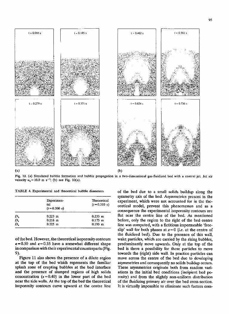
Figures 10(a) and 10(b) show a sequence of density plots which illustrate the propagation of the first bubbles through the fluidized bed. These plots have been ob- tained from the calculated instantaneous solidity dis- tributions according to the procedure described in Kuipers et al. [19]. A comparison with Fig. 7 shows that the theoretical calculation correctly predicts the formation and propagation of a relatively large start- up bubble and subsequent evolution of small elongated bubbles at the jet mouth.

A comparison between the experimental (at t =0.300 s) and theoretical (at t =0.310 s) bubble diameters is presented in Table 4. The close agreement between the experimental data and the predictions from the hydrodynamic model is remarkable. Similar to the ex- periment, the simulation also shows phenomena such as bubble growth (partly due to bubble coalescence) and bubble splitting. However, the agreement between experiment and theory is not perfect, which can be expected at this stage of theoretical development.

For example, the theoretical model assumes New- tonian behaviour of the dense phase, which must be regarded as a first approximation to the true rheological behaviour of fluidized suspensions. Furthermore, the discrepancies between experiment and theory can be attributed, to some extent, to asymmetries present in the experiment. Symmetry about thevertical line passing through the jet centre (i.e. the centre line of the fluidized bed) has been assumed in the computer simulation duplicating the experiment.

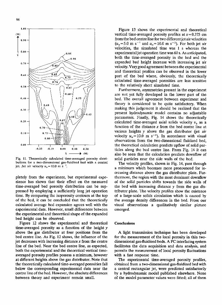
Figure 11 shows the theoretically calculated time- averaged porosity contours for a jet velocity ZQ,= 10.0 m s-l. The isoporosity contours shown in Fig. 11 have been obtained by simple linear interpolation of the time-averaged porosities which were calculated at the centres of the computational cells. In accordance with the experimental results (Fig. 9), the theoretical cal- culation shows the existence of elliptic isoporosity con- tours (E = 0.80, E = 0.75 and E= 0.70) near the jet region. However, the calculated time-averaged isoporosity con- tours indicate a somewhat weaker penetration of the jet into the fluidized bed.

From Fig. 11 it can further be seen that very strong lateral porosity gradients exist near the dilute jet region. These gradients decrease with increasing distance y above the gas distributor. Similar to the experiment, the isoporosity contours l =0.45, l =0.50, ~=0.55 and l =0.60 emanate from the jet mouth and reach the top of the bed, where they deflect towards the side walls

t = 0.093 s t= 0.185 s

(4

t = 0.462 s t= 0.561 s I------

t = 0.654 s t = 0.736 s

Fig. 10. (a) Simulated bubble formation and bubble propagation in a two-dimensional gas-fluidized bed with a central jet. Jet air velocity u,=lO.O m s-‘; (b) see Fig. 10(a).

TABLE 4. Experimental and theoretical bubble diameters

Experimen- tal (t=0.300 s)

Theoretical (t= 0.310 s)

Dh 0.223 m 0.233 m D” 0.218 m 0.173 m DC 0.225 m 0.193 m

of the bed. However, the theoretical isoporosity contours E = 0.50 and E= 0.55 have a somewhat different shape in comparison with their experimental counterparts (Fig.

9). Figure 11 also shows the presence of a dilute region

at the top of the bed which represents the familiar splash zone of erupting bubbles at the bed interface and the presence of slumped regions of high solids concentration (E= 0.40) in the lower part of the bed near the side walls. At the top of the bed the theoretical isoporosity contours curve upward at the centre line

of the bed due to a small solids buildup along the symmetry axis of the bed. Asymmetries present in the experiment, which were not accounted for in the the- oretical model, prevent this phenomenon and as a consequence the experimental isoporosity contours are flat near the centre line of the bed. As mentioned before, only the region to the right of the bed centre line was computed, with a fictitious impermeable ‘free- slip’ wall for both phases at x= 0 (i.e. at the centre of the fluidized bed). Due to the presence of this wall, wake. particles, which are carried by the rising bubbles, predominantly move upwards. Only at the top of the bed is there a possibility for these particles to move towards the (right) side wall. In practice particles can move across the centre of the bed due to developing asymmetries and consequently no solids buildup occurs. These asymmetries originate both from random vari- ations in the initial bed conditions (incipient bed po- rosity) and from the slightly non-uniform distribution of the fluidizing primary air over the bed cross-section. It is virtually impossible to eliminate such factors com-

96

1.00

CM)

T O.YO

0.x0

Y

0.70

0.60

0.50

0.40

0.30

0.20

0. IO

0.00

-0.20 -0.10 0.00 0.10 Q.20

X - CM)

Fig. 11. Theoretically calculated time-averaged porosity distri- butions for a two-dimensional gas-fluidized bed with a central jet. Jet air velocity u,=lO.O m s-l.

pletely from the experiment, but experimental expe- rience has shown that their effect on the measured time-averaged bed porosity distribution can be sup- pressed by employing a sufficiently long jet operation time. By comparing the isoporosity contours at the top of the bed, it can be concluded that the theoretically calculated average bed expansion agrees well with the experimental data. However, small differences between the experimental and theoretical shape of the expanded bed height can be observed.

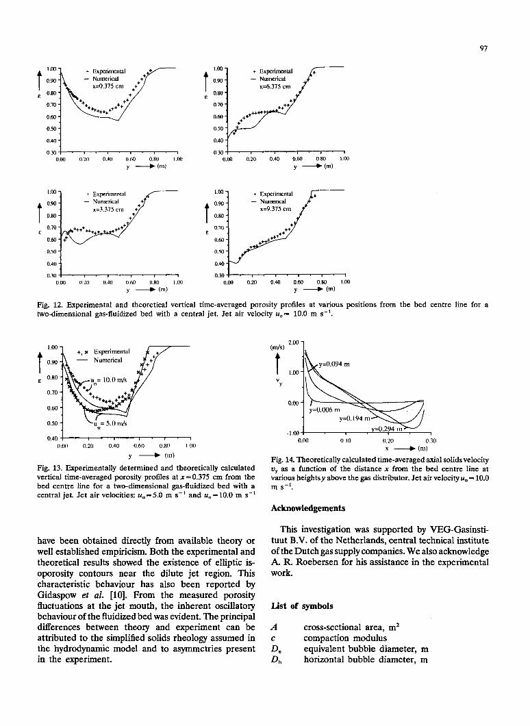
Figure 12 shows the experimental and theoretical time-averaged porosity as a function of the height y above the gas distributor at four positions from the bed centre line. As Fig. 12 shows, the influence of the jet decreases with increasing distance x from the centre line of the bed. Near the bed centre line, as expected, both the experimental and the theoretical vertical time- averaged porosity profiles possess a minimum, however at different heights above the gas distributor. Note that the theoretically calculated time-averaged porosities fall below the corresponding experimental data near the centre line of the bed. However, the absolute differences between theory and experiment remain small.

Figure 13 shows the experimental and theoretical vertical time-averaged porosity profiles at x = 0.375 cm from the bed centre line for two different jet air velocities (u0=5.0 m s-l and U, = 10.0 m s-l). For both jet air velocities, the simulated time was 1 s whereas the experimental jet operation time was 60 s. As anticipated, both the time-averaged porosity in the bed and the expanded bed height increase with increasing jet air velocity. Very good agreement between the experimental and theoretical profiles can be observed in the lower part of the bed where, obviously, the theoretically calculated time-averaged porosities are less sensitive to the relatively short simulated time.

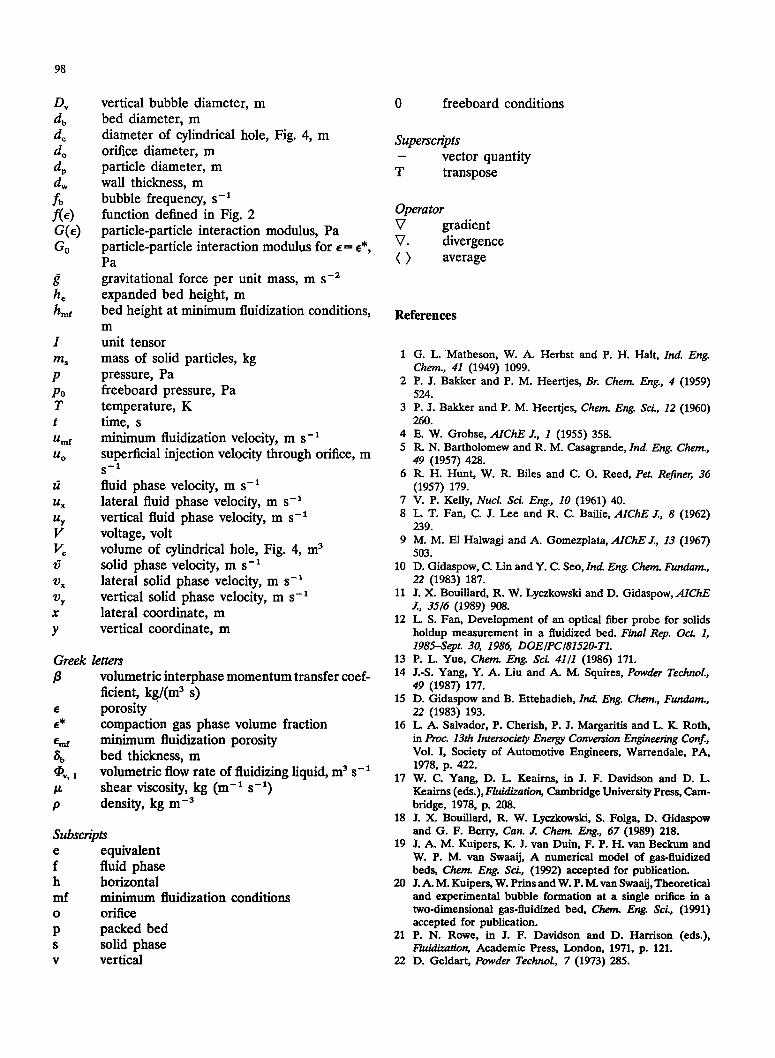
Furthermore, asymmetries present in the experiment are not yet fully developed in the lower part of the bed. The overall agreement between experiment and theory is considered to be quite satisfactory. When making this judgement it should be realized that the present hydrodynamic model contains no adjustable parameters. Finally, Fig. 14 shows the theoretically calculated time-averaged axial solids velocity o, as a function of the distance x from the bed centre line at various heights y above the gas distributor (jet air velocity uO= 10.0 m s-l). In accordance with visual observations from the two-dimensional fluidized bed, the theoretical calculation predicts upflow of solid par- ticles along the bed centre line. From Fig. 14 it can also be seen that the calculation predicts downflow of solid particles near the side walls of the bed.

The velocity profiles, shown in Fig. 14, pass through a minimum which becomes more pronounced for in- creasing distance above the gas distributor plate. Fur- thermore, the region with the most dominant downflow of the solid particles shifts towards the side walls of the bed with increasing distance y from the gas dis- tributor plate. The velocity profiles show the existence of a large-scale solids circulation which is caused by the average density differences in the bed. From our visual observations a qualitatively similar picture emerged.

Conclusions

A light transmission technique has been developed for the measurement of the local porosity in thin two- dimensional gas-fluidized beds. A PC interfacing system facilitates the data acquisition and data analysis, and permits the measurement of local porosity fluctuations with a fast response time.

The experimental time-averaged porosity profiles, obtained from a two-dimensional gas-fluidized bed with a central rectangular jet, were predicted satisfactorily by a hydrodynamic model published elsewhere. None of the model parameter values were fitted; all of them

97

- NumericaJ

0.30 I ’ n . I ’ I . I . 1 0.00 0.20 0.40 0.m 0.80 I .m

y d Cm)

- Numerical

0.40 -

0.30 1 1 . I u I 1 0.00 0.20 0.40 0.60 0.80 I.00

y d Cm)

- Numerical

0.30-t . 1 ’ 1 1 I ’ 1 ’ 1 0.00 0.20 0.40 0.60 0.80 1.00

y ---b Cm)

Fig. 12. Experimental and theoretical vertical time-averaged porosity profiles at various positions from the bed centre line for a two-dimensional gas-fluidized bed with a central jet. Jet air velocity u,= 10.0 m s-r.

1.00

1 0.90

E 0.80

0.70

+, x Experime~nal - Numerical

Fig. 13. Experimentally determined and theoretically calculated vertical time-averaged porosity protiles at x=0.375 cm from the bed centre line for a two-dimensional gas-fluidized bed with a central jet. Jet air velocities: u,=S.O m s-’ and u,= 10.0 m s-r

have been obtained directly from available theory or well established empiricism. Both the experimental and theoretical results showed the existence of elliptic is- oporosity contours near the dilute jet region. This characteristic behaviour has also been reported by Gidaspow et al. [lo]. From the measured porosity fluctuations at the jet mouth, the inherent oscillatory behaviour of the fluidized bed was evident. The principal differences between theory and experiment can be attributed to the simplified solids rheology assumed in the hydrodynamic model and to asymmetries present in the experiment.

I y=O.OY4 m 1.00 -

” Y :b 0.00 -

y=O.W6 nl y=o. 194 m /

-1.00 ! y=O.294 II~ 8

0.00 0.10 0.20 0.30 x - (Ill)

Fig. 14. Theoretically calculated time-averaged axial solidsvelocity q as a function of the distance x from the bed centre line at various heightsy above the gas distributor. Jet air velocity u, = 10.0 m s-l.

Acknowledgements

This investigation was supported by VEG-Gasinsti- tuut B.V. of the Netherlands, central technical institute of the Dutch gas supply companies. We also acknowledge A. R. Roebersen for his assistance in the experimental work.

List of !Symbols

A cross-sectional area, mz

L compaction modulus

6 equivalent bubble diameter, m horizontal bubble diameter, m

98

I? he hti

I

m, P PO T t U mf

UO

vertical bubble diameter, m bed diameter, m diameter of cylindrical hole, Fig. 4, m orifice diameter, m particle diameter, m wall thickness, m bubble frequency, s-’ function defined in Fig. 2 particle-particle interaction modulus, Pa particle-particle interaction modulus for E= E*, Pa gravitational force per unit mass, m s-’ expanded bed height, m bed height at minimum fluidization conditions, m unit tensor mass of solid particles, kg pressure, Pa freeboard pressure, Pa temperature, K time, s minimum fluidization velocity, m s-l superficial injection velocity through orifice, m S-l

fluid phase velocity, m s-l lateral fluid phase velocity, m s-l vertical fluid phase velocity, m s-l voltage, volt volume of cylindrical hole, Fig. 4, m3 solid phase velocity, m s-l lateral solid phase velocity, m s-l vertical solid phase velocity, m s-l lateral coordinate, m vertical coordinate, m

Greek letters P volumetric interphase momentum transfer coef-

ficient, kg/(m3 s) E porosity E* compaction gas phase volume fraction

l mf minimum fluidization porosity

s, bed thickness, m @ “9 I volumetric flow rate of fluidizing liquid, m3 s-l

h shear viscosity, kg (m-l s-l)

P density, kg mm3

Subscripts

H equivalent fluid phase

h horizontal mf minimum fluidization conditions 0 orifice

P packed bed S solid phase V vertical

0 freeboard conditions

Superscripts - vector quantity T transpose

Operator V gradient 8. divergence

0 average

References

1

2

3

4 5

6

7 8

9

10

11

12

13 14

15

16

17

18

19

20

21

22

G. L. Matheson, W. A. Herbst and P. H. Halt, Ind. Eng. Chem., 41 (1949) 1099. P. J. Bakker and P. M. Heertjes, Br. Chem. Eng., 4 (1959) 524. P. J. Bakker and P. M. Heertjes, C/rem. Eng. Sci., 12 (1960) 260. E. W. Grohse, AIChE J., 1 (1955) 358. R. N. Bartholomew and R. M. Casagrande, Znd. Eng. Gem., 49 (1957) 428. R. H. Hunt, W. R. Biles and C. 0. Reed, Pet. Refiner, 36 (1957) 179. V. P. Kelly, Nucl. Sci. Eng., 10 (1961) 40. L. T. Fan, C. J. Lee and R. C. Bailie, AIChE J., 8 (1962) 239. M. M. El Halwagi and A. Gomezplata, AIChE J., 13 (1967) 503. D. Gidaspow, C. Lin and Y. C. Seo, Ind. Eng. Chem. Fundam., 22 (1983) 187. J. X. Bouiiiard, R. W. Lyczkowski and D. Gidaspow, AZChE 1, 3516 (1989) 908. L S. Fan, Development of an optical fiber probe for solids holdup measurement in a fluidized bed. Final Rep. Oct. 1, 198S-Sept. 30, 1986, DOEIPC/8152O_Tl. P. L. Yue, Chem Eng. Sci. 41/l (1986) 171. J.-S. Yang, Y. A. Liu and A. M. Squires, Powder Technol., 49 (1987) 177. D. Gidaspow and B. Ettehadieh, Ina! Eng. Chem., Fundam., 22 (1983) 193. L. A. Salvador, P. Cherish, P. J. Margaritis and L. K. Roth, in Rec. 13th Intersociety Energy Conversion Engineering Co& Vol. I, Society of Automotive Engineers, Warrendale, PA, 1978, p. 422. W. C. Yang, D. L. Keaims, in J. F. Davidson and D. L Keaims (eds.), Fluidization, Cambridge University Press, Cam- bridge, 1978, p. 208. J. X. Bouillard, R. W. Lyczkowski, S. Folga, D. Gidaspow and G. F. Berry, Can Z Chem. Eng., 67 (1989) 218. J. A. M. Kuipers, K. J. van Duin, F. P. H. van Be&urn and W. P. M. van Swaaij, A numerical model of gas-fluidiied beds, Chem. Eng. Sci., (1992) accepted for publication. J. A. M. Kuipers, W. Prim and W. P. M. van Swaaij, Theoretical and experimental bubble formation at a single orifice in a two-dimensional gas-fluidized bed, Chem. Eng Sk, (1991) accepted for publication. P. N. Rowe, in J. F. Davidson and D. Harrison (eds.), Fluidiz&icn, Academic Press, London, 1971, p. 121. D. Geldart, Powder TechnoL, 7 (1973) 285.

99

23 E.-U. Hartge, Y. Li and J. Werther, in P. Basu and J. F. 25 J. A. M. Kuipers, A two-fluid micro balance model of fluidized Large (eds.), CirculatingFluidized Bed Technology II, Pergamon, beds, Ph.D. Dissertation, Twente University of Technology, Oxford, 1988, p. 153. The Netherlands, 1990.

24 R. Sprung, B. Thomas, Y. A. Liu and A. M. Squires, in K. 26 K. Schiigerl, M. Merz and F. Fetting, Chem. Eng. Sci., 15 Ostergaard and A. Sorensen (eds.), Fluidization, Engineering (1961) 1. Foundation, New York, NY, 1986, p. 409. 27 J. R. Grace, Can. J. Chem. Eng., 48 (1970) 30.