An Experimental Study on Levee Failure Caused by Seepage ...

Experimental and Numerical Study of Rainfall Induced Slope Failure
Ram Krishna REGMI*, Hajime NAKAGAWA, Kenji KAWAIKE, Yasuyuki BABA and
Hao ZHANG
* Department of Civil and Earth Resources Engineering, Kyoto University
Synopsis
The purpose of this study was to predict the failure surface of a slope due to
rainfall. Numerical and experimental study was performed to investigate the mechanism
of the slope failure. Slope stability analysis was carried out in three dimensions using
the pore water pressure and the moisture content calculated by three dimensional
seepage flow model. Only a conventional water-phase seepage flow model as well as the
water-air two-phase seepage flow model, coupled with two dimensional surface flow
and erosion/deposition model, were used for seepage analysis. In numerical analysis, the
influence of pore air on seepage and slope stability was found to be less significant.
Keywords: seepage analysis, variably saturated soil, slope stability, failure surface
1. Introduction
Slope failures in residual soils are common in
many tropical countries particularly during periods
of intense rainfall. The location of the groundwater
table in these slopes may be in deep below the
ground surface and the pore-water pressures in the
soil above the groundwater table are negative to
atmospheric conditions. This negative pore-water
pressure, referred to as matric suction when
referenced to the pore-air pressure that contributes
towards the stability of unsaturated soil slopes
(Fredlund and Rahardjo, 1993; Rahardjo et al.,
1995; Griffiths and Lu, 2005). Under the influence
of rainfall infiltration, water seepage can cause a
gradual loss of matric suction in an unsaturated soil
slope. As the hydraulic properties of the soil with
respect to matric suction are often highly nonlinear,
rapid changes in pore-water pressure have a
significant effect on the soil strength, and therefore
on the stability of the slope.
Rainfall-induced slope failures are generally
caused by increased pore pressures and seepage
forces during periods of intense rainfall (Terzaghi
1950; Sidle and Swanston 1982; Sitar et al. 1992;
Anderson and Sitar 1995; Wang and Sassa 2003).
The effective stress in the soil will be decreased due
to the increased pore pressure and thus reduces the
soil shear strength, eventually resulting in slope
failure (Brand 1981; Brenner et al. 1985). In
tropical areas, slope failures due to rainfall
infiltration are quite usual. These slopes remain
stable for a long time before the rainstorms (Brand
1984; Toll 2001). During the rainfall, a wetting
front goes deeper into the slope, resulting in a
gradual increase of the water content and a decrease
of the negative pore-water pressure. This negative
pore-water pressure is referred to as matric suction
when referenced to the pore air pressure that
contributes towards the stability of unsaturated soil
slopes. The loss of suction causes a decrease in
shear strength of the soil on the potential failure
surface and finally triggers the failure (Rahardjo et
al. 1995; Ng and Shi 1998).
京都大学防災研究所年報 第 54 号 B 平成 23 年 6 月
Annuals of Disas. Prev. Res. Inst., Kyoto Univ., No. 54 B, 2011
― 549 ―

During intense rainfall events the variations in
pore water pressures distributed within the soil are
highly variable depending on the hydraulic
conductivity, topography, degree of weathering,
and fracturing of the soil. Pore water pressure
increases may be directly related to rainfall
infiltration and percolation or may be the result of
the build-up of a perched or groundwater table
(Terlien, 1998). The response of the material
involved is largely dependent on its permeability. In
high-permeability soils the build-up and dissipation
of positive pore pressures during intense
precipitation events could be very rapid (Johnson
and Sitar, 1990). In these cases slope failures are
caused by high intensity rainfall and antecedent
rainfall has little influence on landslide occurrence
(Corominas, 2001). On the contrary, in
low-permeability soils slope failures are caused by
long duration-moderate intensity rainfall events; in
fact, the reduction in soil suction and the increase in
pore water pressures due to antecedent rainfall,
considered a necessary condition for landslide
occurrence (Sanderson et al., 1996; Wieczorek,
1987).
Various physically based models coupling the
infinite slope stability analysis with the
hydrological modeling were developed assuming
steady or quasi-steady water table and groundwater
flows parallel to hill slope (Montgomery and
Dietrich 1994; Wu and Sidle 1995; Borga et al.
1998). With approximation of Richards’ equation
(1931) valid for hydrological modeling in nearly
saturated soil, Iverson (2000) further developed a
flexible modeling framework of shallow landslide.
Baum et al. (2002) proposed an extension version
of Iverson’s model to consider variable rainfall
intensity into account for hill slope with finite depth.
Tsai and Yang (2006) modified Iverson’s model by
amending the boundary condition at the top of the
hill slope to consider more general infiltration
process instead of constant infiltration capacity.
The physically based model with the hydrological
modeling in nearly saturated soil (Iverson 2000;
Baum et al. 2002; Tsai and Ynag 2006) was
commonly used for the assessment of shallow
landslides triggered by rainfall due to its simplicity
(Crosta and Frattini 2003; Keim and Skaugset 2003;
Frattini et al. 2004; Lan et al. 2005; D’Odorico et al.
2005; Tsai 2007). Tsai et al. (2008) developed a
physically based model not only by using the
complete Richards’ equation with the effect of
slope angle, but also by adopting the extended
Mohr-Coulomb failure criterion (Fredlund et al.
1978) to describe the unsaturated shear strength.
Sassa (1972, 1974) carried out a series of flume
tests and concluded that the changes in rigidity of
sand and upper yield strain within a slope are
essential to the analysis of slope stability. Fukuzono
(1987) conducted experiment to examine the
conditions leading up to slope failure using nearly
actual-scale slope models providing heavy rainfall.
Crozier (1999) tested a rainfall-based
landslide-triggering model developed from previous
landslide episodes in Wellington City, NewZealand,
which referred to as the Antecedent Water Status
Model, to provide a potentially useful level of
prediction of landslide occurrence by providing a
24-hour forecast. Sharma (2006) carried out
experimental and numerical studies to investigate
effects of slope angle on the moisture movement on
unsaturated soil and further on the slope stability,
and also analyzed the difference in failure pattern
and moisture movement in single and two layers of
soil with different hydraulic conductivities.
Tsustumi and Fujita (2008) investigated several
landslide sites and used physical experiment and
numerical simulation with the combination of
rainwater infiltration for the analysis of slope
stability. Mukhlisin and Taha (2009) developed
numerical model to estimate the extent of rainwater
infiltration into an unsaturated slope, the formation
of a saturated zone, and the change in slope stability.
Then, the model was used to analyze the effects of
soil thickness on the occurrence of slope failure.
The above discussed numerical studies are
applicable only for two dimensional analyses;
however failure of slopes occurs in three
dimensions. There is not only water phase but also
air phase in soil slopes. Both the pore air and pore
water will have influence on the seepage flow, but
all the above mentioned studies have neglected the
air flow on seepage analysis. In looking at the
behaviour of unsaturated soils, some authors (e.g.
Dakshanamurthy et al, 1984) incorporate airflow
within the soil, and it is clear that this aspect can be
significant to the overall behaviour of the soil.
― 550 ―

Therefore, numerical study in three dimensions is
necessary for seepage analysis and slope stability
analysis with considering the effects of air phase in
the seepage.
In this study the analysis of slope failure due to
rainfall was investigated using pore water pressure
and moisture content calculated by only a
conventional water-phase seepage flow model as
well as the water-air two-phase seepage flow model.
Janbu’s simplified method was incorporated into
dynamic programming to locate the critical slip
surface of a general slope. Simulation results were
compared with the experimental results obtained so
as to evaluate the capability of the model.
2. Numerical Modeling
Numerical models can be valuable tools in the
prediction of seepage and the slope stability
analysis. In the present analysis single-phase
seepage flow model calculates the pore water
pressure and moisture content inside the body of the
considered model slope where as the two-phase
model calculates the pore water pressure, pore air
pressure, and moisture content. Necessary surface
water head for the seepage flow model was
evaluated using surface flow and erosion/deposition
model. Slope stability model uses the pore water
pressure and moisture content obtained by the
seepage flow model as well as surface water head
obtained by the surface flow and erosion/deposition
model as in put data to calculate the critical slip
surface and the corresponding factor of safety
simultaneously.
2.1 Seepage flow model
Following pressure based Richards’ equation
valid for variably saturated soil was used in
conventional 3D seepage flow model for calculating
the change in pore water pressure inside the model
slope (Awal et al., 2009).
+
∂
∂
∂
∂+
∂
∂
∂
∂
+
∂
∂
∂
∂=
∂
∂
+
1z
h
zK
zy
h
yK
y
x
h
xK
xt
h
sS
wSC
ww
ww
(1)
where, hw is the water pressure head; Kx, Ky and
Kz are the hydraulic conductivity in x, y and z
direction respectivel; C=∂θw/∂hw is the specific
moisture capacity, θw is the soil volumetric water
content; Sw is the saturation ratio; Ss is the specific
storage; t is the time; x and y are the horizontal
spatial coordinates; and z is the vertical spatial
coordinate taken as positive upwards.
In order to solve the equation (1) following
constitutive relationships proposed by van
Genuchten (1980) are used for establishing
relationship of moisture content and water pressure
head (θw-h), and unsaturated hydraulic conductivity
and moisture content(K-θw):
mwe hS
−+= ])(1[ ηα (2)
rs
rweS
θθ
θθ
−
−=
(3)
2/15.0])1(1[ mm
ees SSKK −−= (4)
where, Se is the effective saturation; α and η are
empirical parameters; θs and θr are saturated and
residual moisture content respectively; Ks is the
saturated hydraulic conductivity; and m=1-1/η.
For 3D water-air two-phase seepage flow
analysis, following equations are derived for the
simultaneous flow of water and air based on the 1D
flow equations (Touma, and Vauclin, 1986).
Water-phase equation
+∂
∂
∂
∂+
∂
∂
∂
∂
+∂
∂
∂
∂=
∂
∂−
∂
∂
1z
wh wzK
zy
whwyK
y
x
whwxK
xt
wh
t
ahC
(5)
Air-phase equation
( )
+∂
∂
∂
∂
+∂
∂
∂
∂+
∂
∂
∂
∂
=∂
∂+
∂
∂−−
owρaρ
z
ah az Kaρ
z
y
ahay Kaρ
yx
ahax Kaρ
x
t
wh Caρ
t
ah Caρ
oh
oaρwθn
(6)
where, ha is the air pressure head; ho is the
atmospheric pressure expressed in terms of water
column height; C= ∂θ/∂hc is the specific moisture
capacity; hc = ha –hw is capillary head; n is the
porosity of soil; ρa is density of air; ρoa is density of
― 551 ―

air at the atmospheric pressure; ρow is density of
water at the atmospheric pressure; Kwx, Kwy and Kwz
are the hydraulic conductivity in x, y and z
directions respectively; and Kax, Kay and Kaz are the
air conductivity in x, y and z directions respectively.
In order to solve the equations (5) and (6)
following constitutive relationships proposed by
van Genuchten (1980) are used:
m
ce hS−+= ])(1[
ηα (7)
rs
rweS
θθ
θθ
−
−= (8)
2/15.0])1(1[ mm
eewsw SSKK −−= (9)
mm
eeasa SSKK 2/15.0 )]1[()1( −−= (10)
where, Kws is the saturated hydraulic
conductivity; Kas=Kws (µw/µa) is the saturated air
conductivity; and µw and µa are dynamic viscosity
of water and air respectively. µw =1.002×10⁻²
NS/m2 and µa =1.83×10⁻⁵ NS/m
2 at 20°c.
Numbers of methods are available for the
numerical solution. In several 1D variably saturated
flow studies, finite difference schemes have been
widely used (e.g. Day and Luthin, 1956; Freeze,
1969; Kirkby, 1978; Dam and Feddes 2000;
Vasconcellos and Amorim, 2001). However, fewer
researchers have used finite differences to solve
variably saturated flow problems in higher
dimensions. In this study, the equations (1), (5) and
(6) are solved by line successive over relaxation
(LSOR) scheme used by Freeze (1971a, 1971b,
1978) by an implicit iterative finite difference
scheme.
2.2 Surface flow and erosion/deposition model
The mathematical model developed by
Takahashi and Nakagawa (1994) was used to
investigate the surface flow and erosion/deposition
on the surface of the model slope. The depth-wise
averaged two-dimensional momentum equations for
the x-wise (down valley) and y-wise (lateral)
directions are:
( ) ( )
( )T
bxbbxobxo
x
zhghgh
y
vM
x
uM
t
M
ρ
τθθ
ββ
−∂
+∂−
=∂
∂+
∂
∂+
∂
∂
cossin
(11)
and
( ) ( )
( )T
bybbyobyo
y
zhghgh
y
vN
x
uN
t
N
ρ
τθθ
ββ
−∂
+∂−
=∂
∂+
∂
∂+
∂
∂
cossin
(12)
The continuity of the total volume is
( ){ }
IR
scciy
N
x
M
t
hbb
−
+−+=∂
∂+
∂
∂+
∂
∂** 1
(13)
The continuity equation of the particle fraction
is
( ) ( ) ( )*ci
y
cN
x
cM
t
chb=
∂
∂+
∂
∂+
∂
∂ (14)
The equation for the change of bed surface
elevation is
bb it
z−=
∂
∂ (15)
where, M (=uh) and N (=vh) are the flow
discharge per unit width in x and y directions; u and
v are depth averaged velocities in x and y
directions; h is the water depth; g is the
gravitational acceleration; β is the momentum
correction factor; ρT is the mixture density; τbx and
τby are the bottom shear stresses in x and y
directions; R is the rainfall intensity; I is the
infiltration rate; sb is the degree of saturation in the
bed; ib is the rate of hydraulic erosion or deposition
from the flowing water; c is the sediment
concentration in the flow; c* is the maximum
sediment concentration in the bed; and zb is the
erosion or deposition thickness measured from the
original bed elevation.
Takahashi (1991) categorized the flow as: a)
stony debris flow (c≥0.4c*), b) immature debris
flow (0.4c*>c≥0.1c*) and c) turbulent flow
(c<0.1c*); based on sediment concentration in the
flow and proposed different flow resistance
equations for each types of flow.
For stony debris flow
23/1*
222
222
2
}1)/}{(/)1({8
8
1
−−+
+
=+
=
cccc
vuu
h
d
vuuh
d
mT
mbx
σρ
ρ
σλτ (16)
― 552 ―

23/1*
222
222
2
}1)/}{(/)1({8
8
1
−−+
+
=+
=
cccc
vuv
h
d
vuuh
d
mT
mby
σρ
ρ
σλτ (17)
For immature debris flow
22
2
49.0vuu
h
dmTbx +
=
ρτ (18)
22
2
49.0vuv
h
dmTby +
=
ρτ (19)
For turbulent flow
3/1
222
h
vuugnbx
+=
ρτ (20)
3/1
222
h
vuvgnby
+=
ρτ (21)
where, n is the Manning's roughness coefficient
and dm is the mean diameter of particles.
The erosion velocity for unsaturated bed given
by Takahashi (1991) is as follows.
( )m
T
T
beb
d
hcc
c
Kgh
i
−
−⋅
−
−−
=
∞1tan
tan
1tan
tan1
sin
2/1
2/3
θ
φ
θ
φ
ρ
ρσ
θ
(22)
where, ø is the internal friction angle of the bed,
Ke is the parameter of erosion velocity and c∞ is the
equilibrium solids concentration. c∞ is defined by
the following equations (Nakagawa et al., 2003).
For stony debris flow (tanθ>0.138)
)tan)(tan(
tan
θφρσ
θρ
−−=∞c (23)
For immature debris flow (0.138≥tanθ>0.03)
2
)tan)(tan(
tan7.6
−−=∞
θφρσ
θρc (24)
For turbulent flow (0.03≥tanθ)
−
−
−
+=∞
*
*0
*
*20 11
1/
tan)tan51(
τ
τα
τ
τα
ρσ
θθ
cc
c
(25)
Where, θ is water surface gradient, and
{ })1//(tan)/(1
)1//(tan)/(425.0220
−−
−−=
ρσθρσ
ρσθρσα (26)
θτ tan72.1* 1004.0 ×=c (27)
md
h
)1/(
tan*
−=
ρσ
θτ (28)
in which τ*c is the non-dimensional critical
shear stress and τ* is the non-dimensional shear
stress.
If the slope is steeper than about 9 degrees and
cs∞ by equation (29) calculates the value less than c∞
27.6 ∞∞= ccs
(29)
and for the slope on which cs∞ by equation (29)
count less than 0.01, cs∞ should be obtained by
using appropriate bed load equation.
The deposition velocity given by Takahashi
(1991) is as follows.
22
*
vuc
cci db +
−= ∞δ (30)
where, dδ is a constant.
The finite difference form of the equations (11)
to (14) can be obtained by the solution methods
developed by Nakagawa (1989) using Leap-Frog
scheme.
2.3 Slope stability model
The stability of a slope depends on its geometry,
― 553 ―

soil properties and the forces to which it is
subjected to internally and externally. The
numerous methods currently available for slope
stability analysis provide a procedure for assigning
a factor of safety to a given slip surface, but do not
consider the problem of identifying the critical
conditions. Limit equilibrium method of slices is
widely used for slope stability analysis due to its
simplicity and applicability. In the method of slices,
the soil mass above the slip surface is divided into a
number of vertical slices and the equilibrium of
each of these slices is considered. The actual
number of the slices depends on the slope geometry
and soil profile. The limiting equilibrium
consideration usually involves two steps; one for
the calculation of the factor of safety and the other
for locating the most critical slip surface which
yields the minimal factor of safety. Methods by
Bishop, Janbu, Spencer and Morgenstern and Price
are now well known.
In this study Janbu’s simplified method has
been incorporated into an effective minimization
procedure based on dynamic programming by
which the minimal factor of safety and the
corresponding critical non circular slip surface are
determined simultaneously. Fig. 1 shows the three
dimensional general slip surface and forces acting
on a typical column. Wij is the weight of column; Pij
is the vertical external force acting at the top of the
column; Tij and Nij are the shear force and total
normal force acting on the column base; Qij is the
resultant of all intercolumn forces acting on the
column sides; �x and �y are discretized widths of
the columns in x and y directions respectively; and
αxz and αyz are the inclination angles of the column
base to the horizontal direction in the xz and yz
planes respectively.
The factor of safety Fs for Janbu’s simplified
method is expressed by the following equation
(Awal et al., 2009).
( )( )
( )
( )∑∑
∑∑
= =
= =
+
+
+
+∆∆−
=m
i
n
j
xzijijij
m
i
n
j
xzij
sxzij
ijij
ijpe
s
PW
FJ
PW
yxuc
F
1 1
1 1
tan
cos
/tansin/1
tan
tan
α
α
φα
φ
φ
(31)
where, ce and ø are the Mohr-Coulomb
strength parameters. J=(1+tan2αxzij + tan2αyzij)1/2;
∑ ∑+= dxdydzcdxdydztzyxW swwij γγθ *),,,(
(the weight of a column);
∑= dxdytyxhP wij ),,(γ (the vertical external force
i.e., surface water weight, acting on the top of the
column); ),,,( tzyxhAverageu wwijp ∑= γ (the
pore water pressure at the base of the column) for
hw(x,y,z,t)>0; dx, dy and dz are the size of cell used
in seepage flow model, γw and γs are the unit weight
of water and solids respectively, c* is the volume
Fig. 1 Three dimensional general slip surface and forces acting on a typical column
(a) Sliding mass and vertically divided columns (b) Forces acting on a the column ij
X
Y
Z
O
Sliding direction
A column
Z
X
Y
Qij
Wij
Tij
Nij
αxzij
αyzij
∆x
∆y
Pij
― 554 ―
concentration of the solids fraction in the body of
slope model, θw(x,y,z,t) and hw(x,y,z,t) are the
moisture content and pressure head in each cell and
h(x,y,z,t) is the depth of surface water above the
cell.
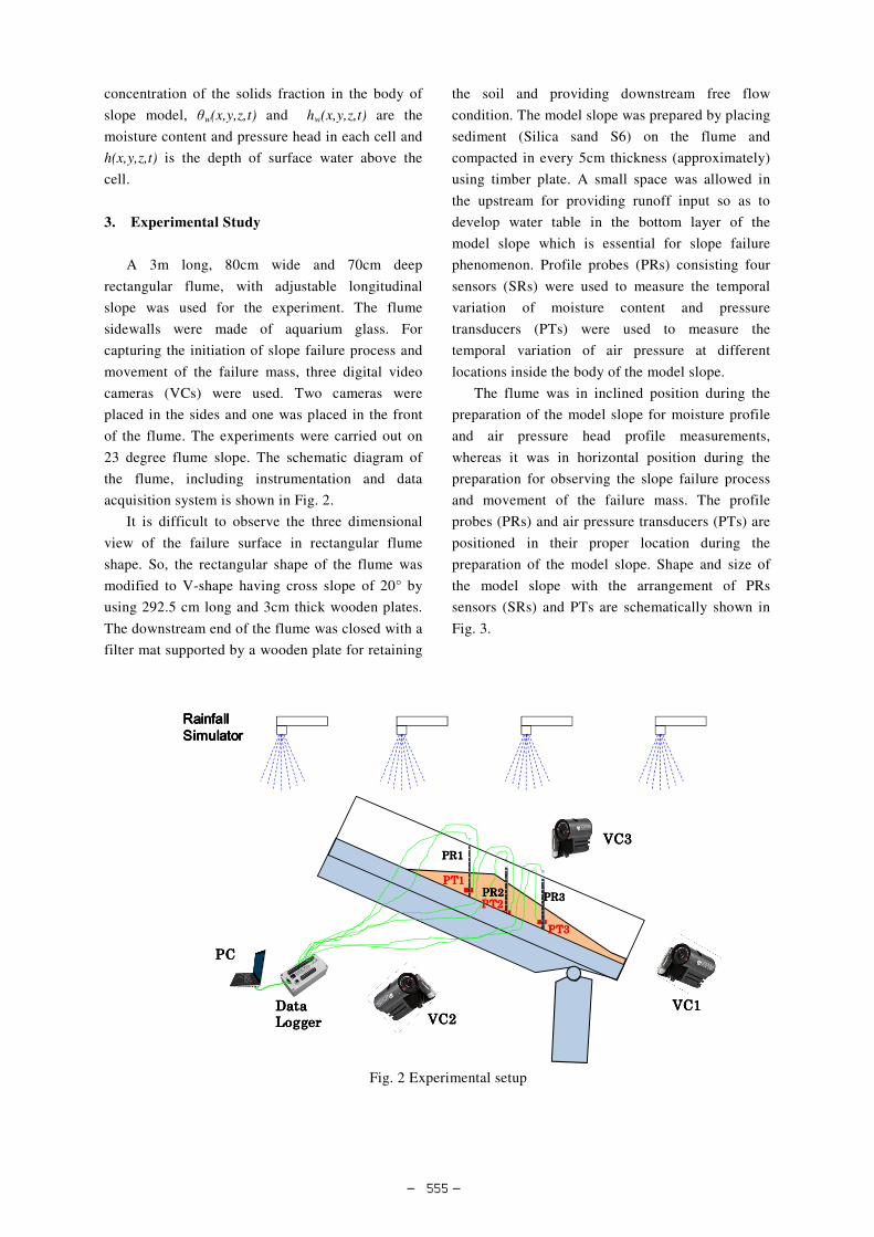
3. Experimental Study
A 3m long, 80cm wide and 70cm deep
rectangular flume, with adjustable longitudinal
slope was used for the experiment. The flume
sidewalls were made of aquarium glass. For
capturing the initiation of slope failure process and
movement of the failure mass, three digital video
cameras (VCs) were used. Two cameras were
placed in the sides and one was placed in the front
of the flume. The experiments were carried out on
23 degree flume slope. The schematic diagram of
the flume, including instrumentation and data
acquisition system is shown in Fig. 2.
It is difficult to observe the three dimensional
view of the failure surface in rectangular flume
shape. So, the rectangular shape of the flume was
modified to V-shape having cross slope of 20° by
using 292.5 cm long and 3cm thick wooden plates.
The downstream end of the flume was closed with a
filter mat supported by a wooden plate for retaining
the soil and providing downstream free flow
condition. The model slope was prepared by placing
sediment (Silica sand S6) on the flume and
compacted in every 5cm thickness (approximately)
using timber plate. A small space was allowed in
the upstream for providing runoff input so as to
develop water table in the bottom layer of the
model slope which is essential for slope failure
phenomenon. Profile probes (PRs) consisting four
sensors (SRs) were used to measure the temporal
variation of moisture content and pressure
transducers (PTs) were used to measure the
temporal variation of air pressure at different
locations inside the body of the model slope.
The flume was in inclined position during the
preparation of the model slope for moisture profile
and air pressure head profile measurements,
whereas it was in horizontal position during the
preparation for observing the slope failure process
and movement of the failure mass. The profile
probes (PRs) and air pressure transducers (PTs) are
positioned in their proper location during the
preparation of the model slope. Shape and size of
the model slope with the arrangement of PRs
sensors (SRs) and PTs are schematically shown in
Fig. 3.
RainfallRainfallRainfallRainfallSimulatorSimulatorSimulatorSimulator
VCVCVCVC1111
VCVCVCVC3333
VCVCVCVC2222
PRPRPRPR1111
PRPRPRPR2222 PRPRPRPR3333
PTPTPTPT1111
PTPTPTPT2222
PTPTPTPT3333
PCPCPCPC
DataDataDataData
LoggerLoggerLoggerLogger
Fig. 2 Experimental setup
― 555 ―

PRPRPRPR1111
PRPRPRPR2222
PRPRPRPR3333
3-D view of the soil mass
SideSideSideSide BBBB
SideSideSideSide AAAA
Soil mass view fromside A
230
330
20
All dimensions are in cm
PTPTPTPT1111SRSRSRSR1111
SRSRSRSR2222
X-section at PR1
SideSideSideSide BBBBSideSideSideSide AAAA
40404040 20202020
200
20202020
10101010
55 55.. .. 55 55
13131313.. .. 22 22
20202020.. .. 77 77
14141414.. .. 55 55
PTPTPTPT2222SRSRSRSR5555
SRSRSRSR6666
SRSRSRSR7777
SRSRSRSR8888
X-section at PR220202020 4040404020202020
10101010
55 55.. .. 77 77
1010101010101010
13131313.. .. 22 22
32323232.. .. 88 88
PTPTPTPT3333SRSRSRSR9999
SRSRSRSR10101010
X-section at PR32020202020202020 2020202020202020
10101010
13131313.. .. 22 22
77 77.. .. 77 77
32323232.. .. 88 88
Fig. 3 Shape and size of the model slope with the arrangement of SRs and PTs
Before Failure
After Failure
Failure Surface
Fig. 4 Typical sketches showing the alignment of threads/sand strips before and after the failure of slope in a
particular L-section
0
10
20
30
40
50
60
70
80
90
100
0.01 0.1 1
S6
Sediment type S6
Saturated moisture content, θs 0.42
Residual moisture content, θr 0.004
Van Genuchten parameter, α 5.719
Van Genuchten parameter, η 5.044
Specific gravity, Gs 2.63
Mean grain size, D50 (mm) 0.24
Angle of repose, ø 340
Porosity, n 0.4221
Compression index, CI 1.08 Particle diameter (mm)
Table 1 Some parameter values of the sediment
Perc
en
t fi
ner
Fig. 5 Grain size distribution of the sediment
― 556 ―

Red colored sediment strips and red colored
cotton threads were placed respectively at the side
wall faces and inside the body, normal to the flume
bed, so as to measure the failure surface after
sliding. Sediment strips were placed at the face of
the flume and threads were attached firmly in the
bottom wall before preparation of the dam body.
Fig. 4 presents the typical sketches showing
alignment of sand strips/threads before and after the
failure of slope in a particular L-section. Some
parameter values of the sediment used are listed in
Table 1. The grain size distribution of the sediment
is shown in Fig. 5.
4. Results and Discussions
Numerical simulation was carried out with time
step of 0.01 second and space steps of 2.5cm,
2.424cm and 2.5cm in x (longitudinal), y (lateral)
and z (vertical) directions respectively. Both x and
y directions were assumed horizontal. In surface
water flow and erosion/deposition model, the time
step of 0.005sec and space steps of 2.5cm and
2.424cm in x (parallel to longitudinal axis of flume)
and y (horizontal) directions respectively. Space
steps of 15cm and 10cm in x (parallel to
longitudinal axis of flume) and y (horizontal)
directions with time step of 10 second was used in
slope stability model.
Average rainfall over the flume during
experiment was 105.365mm/hr. Fig. 6 shows the
rainfall distribution over the flume. In simulation,
same rainfall distribution was used. Fig. 7 shows
the experimental and simulated air pressure head
profiles at the position of different PTs. Fig. 8
shows the experimental and simulated moisture
profiles at the position of different SRs.
Essentially air becomes trapped in the voids by
the infiltrating water from the surface, initially
causing compression of the air phase, leading to a
reduction in the rate of water infiltration. The air
pressure will increase until it reaches a sufficient
value for the air to escape by bubbling. Moisture
profiles obtained considering two-phase flow was
found a little bit delayed in comparison with that of
one-phase flow (Fig. 8).
131131131131....89898989 97979797....09090909 89.36 109.98 73.03 67676767....02020202 104.83 97.09
144144144144....01010101 81.63 74.75 121.16 108.26 92.79 133.61 65.30
152152152152....94949494 70.03 88.50 177.86 99.67 143.92 133.61 64.44
3333....0000mmmm
33 33 00 0033 33 00 00
33 33 00 00cm
cm
cm
cm
45454545
88 88 00 00cm
cm
cm
cm
45454545 45454545 45454545 45454545 45454545 45454545 45454545cmcmcmcm
Fig. 6 Distribution of rainfall intensity (in mm/hr) over the flume
0
5
10
15
20
25
0 1000 2000 3000
EXP-PT1
SIM-PT1
0
5
10
15
20
25
0 1000 2000 3000
EXP-PT2
SIM-PT2
0
5
10
15
20
25
0 1000 2000 3000
EXP-PT3
SIM-PT3
Fig. 7 Experimental and simulated air pressure head profiles
Flume boundary
Time (sec)
Pre
ssu
re h
ead
(cm
)
Time (sec)
Pre
ssu
re h
ead
(cm
)
Time (sec)
Pre
ssu
re h
ead
(cm
)
― 557 ―

0
10
20
30
40
50
60
70
80
90
100
0 500 1000 1500 2000 2500 3000
EXP-SR1
EXP-SR2
EXP-SR5
EXP-SR6
EXP-SR7
EXP-SR8
EXP-SR9
EXP-SR10
SIM(1PH)-SR1
SIM(1PH)-SR2
SIM(1PH)-SR5
SIM(1PH)-SR6
SIM(1PH)-SR7
SIM(1PH)-SR8
SIM(1PH)-SR9
SIM(1PH)-SR10
SIM(2PH)-SR1
SIM(2PH)-SR2
SIM(2PH)-SR5
SIM(2PH)-SR6
SIM(2PH)-SR7
SIM(2PH)-SR8
SIM(2PH)-SR9
SIM(2PH)-SR10
Fig. 8 Experimental and simulated moisture profiles
1
1.5
2
2.5
0.5 1 1.5 2 2.5 3 3.5
MODEL SURFACE
FLUME BED
EXP Failure Surface
SIM Failure Surface
1
1.5
2
2.5
0.5 1 1.5 2 2.5 3 3.5
MODEL SURFACE
FLUME BED
EXP Failure Surface
SIM Failure Surface
1
1.5
2
2.5
0.5 1 1.5 2 2.5 3 3.5
MODEL SURFACE
FLUME BED
EXP Failure Surface
SIM Failure Surface
1
1.5
2
2.5
0.5 1 1.5 2 2.5 3 3.5
MODEL SURFACE
FLUME BED
EXP Failure Surface
SIM Failure Surface
1
1.5
2
2.5
0.5 1 1.5 2 2.5 3 3.5
MODEL SURFACE
FLUME BED
EXP Failure Surface
SIM Failure Surface
Fig. 9 Experimental and simulated critical slip surfaces (Time= 2780 second)
Time (sec)
Satu
rati
on
(%
)
Ele
vati
on
(m
)
Distance (m)
Ele
vati
on
(m
)
Distance (m)
Ele
vati
on
(m
)
Distance (m)
Ele
vati
on
(m
)
Distance (m)
Ele
vati
on
(m
)
Distance (m)
Side A 20cm from Side A
40cm from Side A (At centre) 60cm from Side A
Side B (80cm from Side A)
― 558 ―

1 1.5 2 2.5 3
1.5
2
0.004
0.054
0.104
0.154
0.204
0.254
0.304
0.354
0.404
1 1.5 2 2.5 3
1.5
2
0.004
0.054
0.104
0.154
0.204
0.254
0.304
0.354
0.404
Ele
vati
on
(m
)
Distance (m)
Ele
vati
on
(m
)
Distance (m)
Ele
vati
on
(m
)
Distance (m)
Ele
vati
on
(m
)
Distance (m)
Fig. 10 Experimental and simulated moisture contents at 1100 second
b) X-section through PR1
a) L-section through centre line
Simulation (1-phase) Simulation (2-phase)
Simulation (2-phase)
Simulation (1-phase)
EXP-SR5
EXP-SR6
EXP-SR7
EXP-SR8
EXP-SR5
EXP-SR6
EXP-SR7
EXP-SR8
EXP-SR1
EXP-SR2
EXP-SR1
EXP-SR2
― 559 ―

In experiment the slope was failed at 2,780
second. Fig. 9 shows the comparison of
experimental and simulated critical slip surfaces at
2780 second. In simulation calculated factor of
safety was 0.737 in case of data obtained by
one-phase as well as 2-phase seepage analysis.
Simulated moisture content contour at 1,100
seconds is presented in Fig. 10. Experimental
moisture contents observed by various profile probe
sensors are also compared with simulated moisture
contents in Fig. 10.
Janbu’s simplified method only satisfies force
equilibrium for the entire sliding mass and assumes
resultant inter-slice forces horizontal where as it
does not satisfy moment equilibrium. Also the
assumption of horizontal resultant inter-slice forces
does not represent its line of action indeed. For the
same critical surface factor of safety obtained by
other methods that also satisfying moment
equilibrium will be higher.
5. Conclusions
In this study slope stability analysis was carried
out using the pore water pressure and the moisture
content calculated by three dimensional seepage
flow model. Only a conventional water-phase
seepage flow model as well as the water-air
two-phase seepage flow model, coupled with two
dimensional surface flow and erosion/deposition
model, were used for seepage analysis. In seepage
analysis, the influence of air on seepage was found
to be less significant. More experimental studies are
necessary to get experimental and simulated results
quite close. The performance of the model can
further be improved by incorporating more rigorous
method of slope stability analysis.
Acknowledgements
The financial support provided by Japan Society
for the Promotion of Science (JSPS) Grant-in-Aid
for Scientific Research (B) 22360197(Hajime
Nakagawa, Kyoto University) to this research is
gratefully acknowledged.
References
Anderson, S.A. and Sitar, N. (1995): Analysis of
rainfall-induced debris flow, Journal of
Geotechnical Engineering, ASCE, Vol.121, No.7,
pp.544-552.
Awal, R., Nakagawa, H., Kawaike, K., Baba, Y.
and Zhang, H. (2009): Three dimensional transient
seepage and slope stability analysis of landslide
dam, Annuals of Disaster Prevention Research
Institute, Kyoto University, No.52B, pp.689-696.
Baum, R.L., Savage, W.Z. and Godt, J.W. (2002):
TRIGRS - a Fortran program for transient rainfall
infiltration and grid-based regional slopestability
analysis, Virginia, US Geological Survey, Open
file report 02-424.
Borga, M., Fontana, G.D., De Ros, D. and Marchi L.
(1998): Shallow landslide hazard assessment
using a physically based model and digital
elevation data, Environmental Geology, Vol.35,
pp.81-88.
Brand, E.W. (1981): Some thoughts on rainfall
induced slope failures, Proceedings of 10th
International Conference on Soil Mechanics and
Foundation Engineering, pp.373-376.
Brand, E.W. (1984): Landslides in Southeast Asia:
a state of the art report, In Proceedings of the 4th
International Symposium on Landslides, Toronto,
Canada, Vol.1, pp.377- 384.
Brenner, R.P., Tam, H.K. and Brand, E.W. (1985):
Field stress path simulation of rain-induced slope
failure, Proceedings of 11th International
Conference on Soil Mechanics and Foundation
Engineering, Vol.2, pp.373-376.
Corominas, J. (2001): Landslides and Climate,
Keynote Lectures from the 8th International
Symposium on Landslides, Vol.4, pp.1-33.
Crosta, G.B. and Frattini, P. (2003): Distributed
modeling of shallow landslides triggered by
intense rainfall, Nat Haz Earth Syst Sci, Vol.3,
pp.81-93.
Crozier, M. J. (1999): Prediction of
rainfall-triggered landslides: a test of the
Antecedent Water Status Model, Earth Surface
Processes and Landforms, Vol.24, pp.825-833.
Dakshanamurthy, V., Fredlund, D.G. and Rahardjo,
H (1984): Coupled three dimensional
consolidation theory of unsaturated porous media,
Proceedings of the fifth international conference
on expansive soils, Adelaide, South Australia.
― 560 ―

Dam, J.C. van and Feddes, R.A. (2000): Numerical
simulation of infiltration, evaporation and shallow
groundwater levels with the Richards equation,
Journal of Hydrology, Vol.233, pp72-85.
Day, P. R. and Luthin, J. N. (1956): A numerical
solution of the differential equation of flow for a
vertical drainage problem, Proceedings, Soil
Science Society of America, Vol. 20, pp. 443-447.
D’Odorico, P., Fagherazzi, S. and Rigon, R. (2005):
Potential for landsliding: dependence on
hyetograph characteristics, J Geophys Res Earth
Surf 110(F1).
Frattini, P., Crosta, G.B., Fusi, N. and Negro, P.D.
(2004): Shallow landslides in pyroclastic soil: a
distributed modeling approach for hazard
assessment, Engineering Geology, Vol.73,
pp.277-295.
Fredlund, D.G., Morgenstern, N.R. and Widger,
R.A. (1978): The shear strength of unsaturated
soils, Canadian Geotechnical Journal, Vol.15,
pp.313-321.
Fredlund, D.G. and Rahardjo, H. (1993): Soil
mechanics for unsaturated soils, John Wiley and
Sons Inc., 517.
Freeze, R.A. (1969): The mechanism of natural
groundwater recharge and discharge 1.
One-dimensional, vertical, unsteady, unsaturated
flow above a recharging and discharging
groundwater flow system, Water Resources
Research, Vol.5, pp.153-171.
Freeze, R.A. (1971a): Three dimensional transient,
saturated unsaturated flow in a groundwater basin,
Water Resour. Res., Vol.7, pp.347-366.
Freeze, R.A. (1971b): Influence of the unsaturated
flow domain on seepage through earth dams,
Water Resour. Res., Vol.7, pp.929-941.
Freeze, R. A. (1978): Mathematical models of
hillslope hydrology, in Kirkby, M. J., ed.,
Hillslope Hydrology, John Wiley, pp. 177-225.
Fukuzono, T. (1987): Experimental study of slope
failure caused by heavy rainfall, Erosion and
Sedimentation in the Pacific Rim, Proceedings of
the Corvallis Symposium, August.
Griffiths, D.V. and Lu, N. (2005): Unsaturated
slope stability analysis with steady infiltration or
evaporation using elasto-plastic finite elements,
Int. J. Numer. Anal. Meth. Geomech., Vol.29,
pp.249-267.
Iverson, R. M. (2000): Landslide triggering by
rainfall infiltration, Water Resources Research,
Vol.36, pp.1987-1910.
Johnson, K. A. and Sitar, N. (1990): Hydrologic
conditions leading to debris-flow initiations,
Canadian Geotechnical Journal, Vol.27,
pp.789-801.
Keim, R.F. and Skaugset, A.E. (2003): Modelling
effects of forest canopies on slope stability,
Hydrol Process, Vol.17, Vol.1457-1467.
Kirkby, M.J. (1978): Hillslope Hydrology, John
Wiley & Sons, 389 pp.
Lan, H.X., Lee, C.F., Zhou, C.H. and Martin, C.D.
(2005): Dynamic characteristics analysis of
shallow landslides in response to rainfall event
using GIS, Environmental Geology, Vol.47,
pp.254-267.
Montgomery, D.R. and Dietrich, W.E. (1994): A
physically based model for the topographic
control on shallow landslide, Water Resources
Research, Vol.30, pp.83-92.
Mukhlisin, M. and Taha, M.R. (2009): Slope
Stability Analysis of a Weathered Granitic
Hillslope as Effects of Soil Thickness, European
Journal of Scientific Research, Vol.30, No.1,
pp.36-44.
Nakagawa, H., Takahashi, T., Satofuka, Y. and
Kawaike, K. (2003): Numerical simulation of
sediment disasters caused by heavy rainfall in
Camuri Grande basin, Venezuela 1999,
Proceedings of the Third Conference on
Debris-Flow Hazards Mitigation: Mechanics,
Prediction, and Assessment, Switzerland,
Rotterdam, pp.671-682.
Ng, C.W.W. and Shi, Q. (1998): A numerical
investigation of the stability of unsurated soil
slopes subjected to transient seepage, Computers
and Geotechnics, Vol.22, No.1, pp.1-28.
Rahardjo, H., Lim, T.T., Chang, M.F. and Fredlund,
D.G. (1995): Shear strength characteristics of a
residual soil, Canadian Geotechnical Journal,
Vol.32, pp.60-77.
Richards, L.A. (1931): Capillary conduction of
liquids in porous mediums, Physics, Vol.1,
pp.318-333.
Sanderson, F., Bakkehoi, S., Hestenes, E., and Lied,
K. (1996): The influence of meteorological factors
on the initiation of debris flows, rockfalls,
― 561 ―
rockslides and rockmass stability, in: Landslides.
Proceedings 7th International Symposium on
Landslides, edited by: Senneset, K., A.A.
Balkema.
Sassa, K. (1972): Analysis on slope stability: I,
Mainly on the basis of the indoor experiments
using the standard sand produced in Toyoura,
Japan, Journal of the Japan Society of Erosion
Control Engineering, Vol.25, No.2, pp.5-17 (in
Japanese with English abstract).
Sassa, K. (1974): Analysis on slope stability: II,
Mainly on the basis of the indoor experiments
using the standard sand produced in Toyoura,
Japan, Journal of the Japan Society of Erosion
Control Engineering, Vol.26, No.3, pp.8-19 (in
Japanese with English abstract).
Sharma, R.H. (2006): Study on integrated modeling
of rainfall induced sediment hazards, Doctoral
Thesis, Kyoto University.
Sidle, R.C. and Swanston, D.N. (1982): Analysis of
a small debris slide in coastal Alaska, Canadian
Geotechnical Journal, Vol.19, pp.167-174.
Sitar, N., Anderson, S.A. and Johnson, K.A. (1992):
Conditions leading to the initiation of
rainfall-induced debris flows, Proceedings of the
Journal of the Geotechnical Engineering Division
Specialty Conference on Stability and
Performance of Slopes and Embankments-II,
ASCE, New York, NY, pp.834-839.
Takahashi T. (1991): Debris flow, Monograph
Series of IAHR, Balkema, pp.1-165.
Takahashi, T. and Nakagawa, H. (1994):
Flood/debris flow hydrograph due to collapse of
natural dam by overtopping, Journal of
Hydroscience and Hydraulic Engineering, JSCE,
Vol.12, No.2, pp.41-49.
Terlien, M. T. J. (1998): The determination of
statistical and deterministic hydrological
landslide-triggering thresholds, Environmental
Geology, Vol.35, pp.2-3.
Terzaghi, K. (1950): Mechanism of landslides, In:
Paige, S. (Ed.), Application of Geology to
Engineering Practice (Berkey Volume),
Geological Society of America, New York,
pp.83-123.
Toll, D.G. (2001): Rainfall-induced landslides in
Singapore, Proc. Institution of Civil Engineers,
Geotechnical Engineering, Vol.149, No.4,
pp.211-16.
Touma, J. and Vauclin, M. (1986): Experimental
and numerical analysis of two-phase infiltration in
a partially saturated soil, Transport in Porous
Media, Vol.1, pp.27-55.
Tsai, T.L. and Yang, J.C. (2006): Modeling of
rainfall-triggered shallow landslide,
Environmental Geology, Vol.50, No.4,
pp.525-534.
Tsai, T.L. (2007): The influence of rainstorm
pattern on shallow landslide, Environmental
Geology.
Tsai, T.L., Chen, H.E. and Yang, J.C. (2008):
Numerical modeling of rainstorm-induced shallow
landslides in saturated and unsaturated soils,
Environmental Geology, Vol.55, pp.1269-1277.
Tsutsumi, D. and Fujita, M. (2008):Relative
importance of slope material properties and timing
of rain fall for the occurance of landslides,
International Journal of Erosion Control
Engineering, Vol.1, No.2.
van Genuchten, M. T. (1980): A closed-form
equation for predicting the hydraulic conductivity
of unsaturated soils, Soil Sci. Soc. Amer. J.,
Vol.48, pp.703-708.
Vasconcellos, C. A. B. de and Amorim,J. C. C.
(2001): Numerical simulation of unsaturated flow
in porous media using a mass conservative model,
em “Proceeding of COBEM. 2001, Fluid
Mechanics”, Vol.8, pp.139-148, Uberlândia, MG.
Wang, G. and Sassa, K. (2003): Pore-pressure
generation and movement of rainfall-induced
landslides; effects on grain size and fine-particle
content, Journal of Engineering Geology, Vol.69,
pp.109-125.
Wieczorek, G. F. (1987): Effect of rainfall intensity
and duration on debris flows in central Santa Cruz
Mountains, California, Geolog. Soc. Amer.,
Reviews in Engineering Geology, Vol.7.
Wu, W. and Slide, R.C. (1995): A distributed slope
stability model for steep forested basins, Water
Resources Research, Vol.31, pp.2097-2110.
― 562 ―

降雨による斜面崩壊に関する実験及び数値解析
Ram Krishna REGMI*・中川一・川池健司・馬場康之・張浩
*京都大学大学院工学研究科
要 旨
本研究は,降雨による斜面崩壊を予測することを目的としている。実験と数値解析により斜面崩壊のメカニズムにつ
いて検討を行った。間隙水圧と含水量を解く3次元浸透流解析によって斜面の安定解析を実施した。従来の水相のみの
浸透流だけでなく,水と空気の2相を解析する浸透流モデルを2次元の表層流および浸食/堆積モデルとカップリングし,
実験へ適用し検証を行った。数値解析により,浸透流と斜面安定において間隙内の空気の影響は小さく,2相で解析す
る必要性が低いことが示された。
キーワード:浸透流解析,飽和土,斜面安定,表層崩壊
― 563 ―