University of South CarolinaScholar Commons

Theses and Dissertations

2017

Experimental and Numerical Investigation ofPressure Drop in Silicon Carbide Fuel Rod forApplication in Pressurized Water ReactorsAhmed Musafi AbirUniversity of South Carolina

Follow this and additional works at: https://scholarcommons.sc.edu/etd

Part of the Mechanical Engineering Commons

This Open Access Thesis is brought to you by Scholar Commons. It has been accepted for inclusion in Theses and Dissertations by an authorizedadministrator of Scholar Commons. For more information, please contact dillarda@mailbox.sc.edu.

Recommended CitationAbir, A. M.(2017). Experimental and Numerical Investigation of Pressure Drop in Silicon Carbide Fuel Rod for Application in PressurizedWater Reactors. (Master's thesis). Retrieved from https://scholarcommons.sc.edu/etd/4127

EXPERIMENTAL AND NUMERICAL INVESTIGATION OF PRESSURE DROP IN SILICON

CARBIDE FUEL ROD FOR APPLICATION IN PRESSURIZED WATER REACTORS

by

Ahmed Musafi Abir

Bachelor of Science

Bangladesh University of Engineering and Technology, 2013

Submitted in Partial Fulfillment of the Requirements

For the Degree of Master of Science in

Mechanical Engineering

College of Engineering and Computing

University of South Carolina

2017

Accepted by:

Jamil A. Khan, Director of Thesis

Tanvir I. Farouk, Reader

Titan C. Paul, Reader

Cheryl L. Addy, Vice Provost and Dean of the Graduate School

ii

© Copyright by Ahmed Musafi Abir, 2017

All Rights Reserved.

iii

ACKNOWLEDGEMENTS

I would like to express my deep gratitude and thanks to my advisor Dr. Jamil Khan,

for his continuous guidance, support, invaluable suggestions and sharing his knowledge

throughout my Masters study. It has been a great privilege and honor for me to work with

him.

I would also like to thank Dr. Leo A. Carrilho from the Westinghouse Company for

his invaluable suggestions and assistance. I also thank Dr. Tanvir I. Farouk and Dr. Titan

C. Paul for officially agreeing to serve as a reader, and for their advice during my research.

Special thanks to graduate friends, Rajib Mahamud, Azzam Salman, Saad Oudah,

Noble Anumbe, Nabeel Abdulrazzaq, Amitav Tikadar, Abdulwahab Alhashem and Bill

Bradley for their suggestions and help.

Finally I would like to thank the Westinghouse Company for funding this research.

iv

ABSTRACT

Spacer grids are used in pressurized water reactors (PWRs) fuel assemblies which

enhances heat transfer from fuel rods. However, there remain regions of low turbulence in

between the spacer grids which contributes to lower heat transfer. To enhance turbulence

in these regions surface roughness is applied on the fuel rod walls. Meyer et al [1] used

empirical correlations to predict heat transfer and friction factor for artificially roughened

fuel rod bundles at high performance light water reactors (LWRs). At present, several types

of materials are being used for fuel rod cladding including zircaloy, uranium oxide, etc.

But researchers are actively searching for new material that can be a more practical

alternative. Silicon carbide (SiC) has been identified as a material of interest for application

as fuel rod cladding [2].

The current study deals with the experimental investigation to find out the friction

factor increase of a SiC fuel rod with 3D surface roughness. The SiC rod was tested at

USC’s Single Heater Element Loop Tester (SHELT) loop. The experiment was conducted

in turbulent flowing Deionized (DI) water at steady state conditions. Measurements of flow

rate and pressure drop were made. The experimental results were also validated by

Computational Fluid Dynamics (CFD) analysis in ANSYS Fluent. To simplify the CFD

analysis and to save computational resources the 3D roughness was approximated as a 2D

one. The friction factor results of the CFD investigation was found to lie within ±8% of the

experimental results. Simulations were also conducted with the energy equation turned on,

v

and a heat generation of 8 kW applied to the rod. A maximum heat transfer enhancement

of 18.4% was achieved at the highest flow rate investigated (i.e. Re=109204).

vi

TABLE OF CONTENTS

Acknowledgements ............................................................................................................ iii

Abstract .............................................................................................................................. iv

List of Tables ..................................................................................................................... ix

List of Figures ..................................................................................................................... x

List of Symbols ................................................................................................................ xiii

List of Abbreviations ........................................................................................................ xv

Introduction................................................................................................... 1

Background review ....................................................................................... 3

Experimental setup ....................................................................................... 6

3.1 Single Heater Element Loop Tester Loop .................................................... 6

3.2 Test Section ................................................................................................... 9

3.3 Silicon Carbide Fuel Rod ............................................................................ 14

3.4 Test Fluid .................................................................................................... 16

3.5 Pump ........................................................................................................... 16

3.6 Flow Meters ................................................................................................ 17

3.7 Heat Exchangers ......................................................................................... 17

3.8 Compressor ................................................................................................. 17

3.9 Valves ......................................................................................................... 18

vii

3.10 Gage Pressure Transmitter ........................................................................ 18

3.11 Differential Pressure Transmitter .............................................................. 18

3.12 Thermocouples .......................................................................................... 18

3.13 Processing System .................................................................................... 19

Test Plan And DATA REDUCTION ......................................................... 21

4.1 Pressure Drop Cold Test ............................................................................. 21

4.2 Test Plan...................................................................................................... 21

4.3 Control Test ................................................................................................ 22

4.4 Data Reduction............................................................................................ 22

4.5 Test Parameter Tolerance ........................................................................... 23

4.6 Uncertainty Analysis ................................................................................... 24

CFD Analysis ............................................................................................. 25

5.1 Flow Domain .............................................................................................. 25

5.2 Meshing....................................................................................................... 28

5.3 Numerical Methods ..................................................................................... 35

5.4 Data Reduction............................................................................................ 40

Results......................................................................................................... 42

6.1 Experimental Results .................................................................................. 42

6.2 Numerical Results ....................................................................................... 43

Conclusion and Future Research ................................................................ 57

7.1 Conclusion .................................................................................................. 57

viii

7.2 Future Research .......................................................................................... 58

References ......................................................................................................................... 59

ix

LIST OF TABLES

Table 5.1 Geometric Parameters ....................................................................................... 28

Table 5.2 Meshing Parameters .......................................................................................... 33

Table 6.1 Results for friction factor for smooth rods........................................................ 53

Table 6.2 Friction Factor results with the rough SiC rod ................................................. 54

Table 6.3 Friction Factor obtained from the CFD Analysis ............................................. 55

Table 6.4 Nusselt Number obtained from CFD analysis compared with Gnielinski

Correlation ........................................................................................................................ 55

Table 6.5 Comparison of friction factor obtained from experiment and CFD analysis for

the SiC Fuel rod ................................................................................................................ 55

Table 6.6 Nusselt Number calculations for the SiC rod ................................................... 56

Table 6.7 % increasein Nusselt Number ........................................................................... 56

x

LIST OF FIGURES

Figure 3.1 Schematic of the SHELT Loop ......................................................................... 7

Figure 3.2 The SHELT Loop at USC ................................................................................. 8

Figure 3.3 Test Section ..................................................................................................... 10

Figure 3.4 Single Simulated Fuel Rod (Dimensions in mm) ............................................ 11

Figure 3.5 Flow Housing (Dimensions in mm) ................................................................ 12

Figure 3.6 Cross Section of the Test Section .................................................................... 13

Figure 3.7 Roughness structure on the SiC Fuel Rod ....................................................... 15

Figure 3.8 (a) Basic Bench Contour Projector used for roughness measurement, (b)

Display of the basic Bench Contour Projector .................................................................. 15

Figure 3.9 Contour plot for the SiC fuel rod surface ........................................................ 16

Figure 3.10 Rosemount Gage and Differential Transmitters ............................................ 19

Figure 3.11 NI Data Acquisition System .......................................................................... 20

Figure 3.12 The LabVIEW Program Interface ................................................................. 20

Figure 5.1 Flow Domain used for CFD Analysis ............................................................. 26

Figure 5.2 3D CAD model of the SiC Fuel Rod ............................................................... 27

Figure 5.3 2D Flow Domain produced in ANSYS DesignModeler ................................. 27

Figure 5.4 Comparison of fully developed laminar and turbulent flow in channel [17] .. 29

Figure 5.5 Experimental Turbulent boundary layer profiles for various .......................... 29

Figure 5.6 Subdivision of Near Wall Region[18] ............................................................. 30

Figure 5.7 Near wall meshing approaches[18] ................................................................. 31

xi

Figure 5.8 Grid Independence study ................................................................................. 33

Figure 5.9 Meshing in rough region ................................................................................. 34

Figure 5.10 Mesh in the transition region between smooth and rough rod ...................... 34

Figure 5.11 Meshing in smooth Region ............................................................................ 34

Figure 5.12 Boundary Conditions ..................................................................................... 38

Figure 5.13 Finite Difference Schemes used for discretization of the various terms in the

governing equations .......................................................................................................... 38

Figure 5.14 Velocity vs. y (elevation) drawn along center of flow domain ..................... 39

Figure 5.15 Locations where pressure drops are measured .............................................. 39

Figure 5.16 Heat Transfer Calculations ............................................................................ 41

Figure 6.1 Comparison of Smooth Friction factor results from experiment with

correlation ......................................................................................................................... 46

Figure 6.2 Comparison of experimental results of friction factor for SiC rod with the

smooth rod. ....................................................................................................................... 46

Figure 6.3 Comparison of friction factor for smooth rod from CFD analysis and

Correlation ........................................................................................................................ 47

Figure 6.4 Comparison of friction factor obtained from Experiment and CFD analysis . 47

Figure 6.5 Comparison of Nusselt No. at the smooth section (y1=0.737 m) from CFD

analysis and Gnielinski Correlation. ................................................................................. 48

Figure 6.6 Pressure contours and streamlines around roughness ..................................... 48

Figure 6.7 Temperature contours and streamlines around roughness structures

(Re=102,436) .................................................................................................................... 49

Figure 6.8 Wall Temperature variation Twr along the rough wall .................................... 49

Figure 6.9 Comparison of Nusselt Number from CFD analysis for smooth .................... 50

Figure 6.10 Contours of Pressure (Pa) in smooth section ................................................. 50

Figure 6.11 Contours of Temperature (K) in smooth section ........................................... 51

Figure 6.12 Contours of Pressure (Pa) in rough section ................................................... 51

xii

Figure 6.13 Contours of Temperature (K) in rough section ............................................. 52

xiii

LIST OF SYMBOLS

𝑈𝑚 Mean Velocity.

𝑄 Flow Rate.

𝐴𝑐 Cross Sectional Area of test section.

𝑟𝑜 Outer Diameter of the test section.

𝑟𝑖 Diameter of the nuclear fuel rod

𝑅𝑒 Reynolds Number.

𝐷ℎ Hydraulic Diameter of the test section.

𝜗 Kinematic viscosity of DI water.

𝑓 Friction factor.

𝛥𝑝 Differential Pressure Drop.

𝛥𝑥 Length.

𝑅𝑒 Reynolds Number.

ρ Density of DI water.

𝑘𝑠 Sand grain roughness height.

𝐶𝑓 Skin friction coefficient.

𝑈𝜏 Wall friction velocity.

𝑦+ Non-dimensional wall distance

𝑇𝑏1 Bulk temperature at the entrance of rough section.

𝑇𝑏2 Bulk temperature at the outlet of the rough section.

xiv

ℎ Heat transfer coefficient.

𝑘𝑓 conductivity of DI water.

𝑁𝑢 Nusselt Number.

𝑃 Prandtl Number.

𝑞′′ Heat flux per unit area.

ℎ Heat transfer coefficient.

𝑇𝑤 Temperature at wall.

𝑁𝑢 Nusselt Number.

𝑞′′ Heat flux per unit area

xv

LIST OF ABBREVIATIONS

CFD ..................................................................................... Computational Fluid Dynamics

CVI ............................................................................................ Chemical Vapor Infiltration

DI .......................................................................................................................... Deionized

LOCA .......................................................................................... Loss of Coolant Accidents

PWR ............................................................................................ Pressurized Water Reactor

RANS ...............................................................................Reynolds Averaged Navier-Stoke

SiC.................................................................................................................Silicon Carbide

SST .................................................................................................... Shear Stress Transport

UO2 ........................................................................................................... Uranium Dioxide

Zr ........................................................................................................................... Zirconium

1

INTRODUCTION

Turbulence is used as a tool to enhance heat transfer from fuel rods in Pressurized

Water Reactors (PWR) fuel rod assemblies. For this purpose, spacer grids are used in the

fuel assemblies. Unfortunately, these only produce a localized turbulence thus the

turbulence along the fuel rod is low. Thus, to enhance the turbulence along the entire length

of the rods different types of surface roughness are used.

Investigators have reported significant improvements in heat transfer by employing

the artificial roughening technique, mainly on surface of circular channels [3]. Structured

artificial roughness acts as a boundary layer disturber in the near-wall turbulent flow

structure to promote higher momentum and heat transport along the surface.

Zirconium (Zr)-based alloys are used universally in water-cooled reactors as

cladding for nuclear fuel. Zirconium-based alloy cladding prevents release of fission

products into the coolant but introduces some limitations to the nuclear reactors design.

These limits are mainly due to Zirconium-based alloy embrittlement through chemical and

radiation damage, early pellet-cladding mechanical interaction, and restricted mechanical

performance and chemical stability at elevated temperature.

Unfortunately use of surface roughening of fuel rods for heat transfer enhancement

has its drawbacks. The surface roughness causes significant rise in the friction factor, which

means that higher pumping costs will be involved. Thus, researchers and scientists are

continuously struggling to come up with surface roughness that will be the most practical

2

and economic for use in PWR fuel rod assemblies. The purpose of the current investigation

is to experimentally quantify the friction factor for a proposed SiC fuel rod with artificial

roughness, and a consequent CFD analysis for validation of the results. And then CFD

model will be used to approximate heat transfer enhancement for the roughness design.

SiC clad fuel rods have been identified as a suitable replacement for the Zr alloys

for a number of their beneficial properties such as lower thermal neutron absorption [4],

corrosion resistance and resistance to hydrogen embrittlement [5], projected stable

response to beyond design basis accidents, such as station blackout accidents approaching

2000˚C [6], and stable response to design basis loss of coolant accidents (LOCA).

However the SiC is a ceramic and it exhibits relatively brittle behaviour compared to the

dilute Zr alloy. To enhance mechnaical properties of SiC it can be fabricated into composite

tubes. Tube samples formed into composites were tested using 4-point flexure and

instrumented impact at room temperature and it was found to enhance the strength and

strain properties of SiC [2]. Another undesirable property of the SiC when compared with

the Zr alloy is that it has a lower conductivity. Thus before the SiC rod is introduced into

reactor cores it should be subjected to careful evaluation.

3

BACKGROUND REVIEW

With the global rise in energy demand and its scarcity researchers around the globe

are trying hard to figure out ways to make energy efficient systems. The effect of surface

roughness on pressure drop has been an area of interest for eminent researches for a very

long time. An increase in roughness increases the friction factor. Nikuradse conducted the

classical series of experiments with pipes roughened by sand grains [7]. He studied the law

of resistance in the Reynolds number range of 104 to 106 for pipes with circular cross

section and different degrees of roughness defined by 𝑘

𝑟 (where k is average projection of

the roughness and r is the radius of pipe). In order to define the law of resistance he divided

the flow conditions into three ranges. In range I for small Reynold No. the resistance factor

is the same for rough and for smooth pipes. In this region the projection of the sand grain

roughness lie totally within the laminar layer. In range II an increase in the resistance factor

was observed for increasing Reynolds number. The thickness of the laminar layer is same

as that of the projections in this range. For the range III the resistance factor is independent

of the Reynolds number . Here all projections of the roughening extend through the laminar

layer. Therefore, he found that the flow resistance in the laminar region was not effected

by the roughness height. However in the transition and turbulent flow region an increase

in flow resistance occurs due to sand grains extending out of the laminar sublayer into the

turbulent region, and production of vortices.

4

Mark Steinke and Satish Kandilkar [8] suggested heat transfer enhancement

techniques in single phase flows which include: flow transition, breakup of boundary layer,

entrance region, vibration, electric fields, swirl flow and mixers. R.J. Firth and L. Meyer

[9] conducted heat transfer and friction factor performance studies in four different types

of artificially roughnened surfaces:

1. Square transverse ribbed

2. Helically ribbed

3. Trapezoidal transverse ribbed

4. Three dimensional surfaces

These surfaces were developed as part of the nuclear reactor programmes with the

objective of improving the rate of heat removal from fuel pins in gas cooled reactors. The

friction factor and the heat transfer studies were conducted under fully turbulent flows of

Reynolds numbers upto 106. The study concluded that the three dimensional surface has

the best overall thermal performance which showed a thermal preformance improvement

of 15% compared with the trapezoidal transverse ribbed surface. However the 3D surface

has the disadvantage that the surface is more sensitive to changes in the surface geometry.

For the transverse trapezoidal roughness there is no advantage. If a roughness is needed

with a low friction factor without a reduction in rib height then the best alternate is the

helically ribbed surface. The square transverse ribbed surface has an overall performance

that compares well with the other surfaces, and the helically ribbed surfaces has a thermal

performance which compares closely with the square ribbed surface.

Li et al [10] experimentally investigated by measuring the heat transfer in two-

dimensional roughness tubes with different roughness heights at various Reynolds

5

numbers. They concluded that there is a maximum Nusselt number ratio for fixed

roughness height with increasing Reynolds number. They concluded that when the

roughness height is more than five times of the viscous sublayer thickness, the flow friction

begins to increase sharply but heat transfer is slowly enhanced. They concluded that the

best heat transfer enhancement for a given pumping power is reached when roughness

height is three times of viscous sub layer thickness.

Ryu et al [11] conducted a computational investigation of turbulent flow in

channels with two-dimensional ribs and three-dimensional blocks. Reynolds-averaged

Navier-Stokes (RANS) equations, coupled with k-ω turbulence model with near-wall

treatment were solved by a finite-volume method. For the two-dimensional rib roughened

channels they conducted a study on four different types of ribs: square ribs, triangular ribs,

semicircular ribs, wavy wall. It was concluded from that study that the square ribs exert

the most resistance among the four shapes considered while wavy wall offers the least. An

extension of this work [12] presented the heat transfer characteristics of turbulent flow in

channels with two-dimensional ribs and three-dimensional blocks. They concluded that the

heat transfer enhancement corresponds to the maximum resistance coefficient for two-

dimensional ribs. The maximum heat transfer is achieved for the square rib, and it

decreases as the shape changes to triangular, to semicircular and to wavy wall.

Carrilho et al [13] conducted a heat transfer and flow resistance study, by both

experimentation and computatoion due to square transverse ribbed surface on a single fuel

rod. His experimental and computational results suggested a heat transfer enhancement of

50%. Umair et al [14] conducted a similar study due to three dimensional diamond shaped

blocks in turbulent flow. He recorded a maximum heat transfer enhancement of 83%.

6

EXPERIMENTAL SETUP

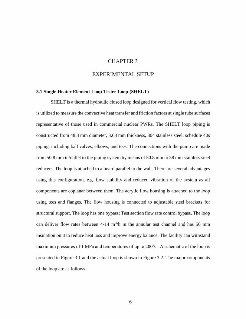
3.1 Single Heater Element Loop Tester Loop (SHELT)

SHELT is a thermal hydraulic closed loop designed for vertical flow testing, which

is utilized to measure the convective heat transfer and friction factors at single tube surfaces

representative of those used in commercial nuclear PWRs. The SHELT loop piping is

constructed from 48.3 mm diameter, 3.68 mm thickness, 304 stainless steel, schedule 40s

piping, including ball valves, elbows, and tees. The connections with the pump are made

from 50.8 mm in/outlet to the piping system by means of 50.8 mm to 38 mm stainless steel

reducers. The loop is attached to a board parallel to the wall. There are several advantages

using this configuration, e.g. flow stability and reduced vibration of the system as all

components are coplanar between them. The acrylic flow housing is attached to the loop

using tees and flanges. The flow housing is connected to adjustable steel brackets for

structural support. The loop has one bypass: Test section flow rate control bypass. The loop

can deliver flow rates between 4-14 m3/h in the annular test channel and has 50 mm

insulation on it to reduce heat loss and improve energy balance. The facility can withstand

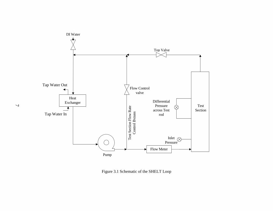
maximum pressures of 1 MPa and temperatures of up to 200˚C. A schematic of the loop is

presented in Figure 3.1 and the actual loop is shown in Figure 3.2. The major components

of the loop are as follows:

7

Figure 3.1 Schematic of the SHELT Loop

Heat

Exchanger

Tap Water In

Tap Water Out

DI Water

Tes

t S

ecti

on F

low

Rat

e

Contr

ol

Bypas

s

Flow Control

valve

Flow Meter

Top Valve

Differential

Pressure

across Test

rod

Inlet

Pressure

Pump

Test

Section

8

Figure 3.2 The SHELT Loop at USC

Heat

Exchanger Pump Flow meter Test Section

9

3.2 Test Section

The test section (Figure 3.3) consists of two (2) major components: the single

simulated fuel rod (Figure 3.4) and the flow housing (Figure 3.5). Specific requirements of

the test section include: 0.2 MPa maximum pressure; 50 C maximum temperature. The

test section performs the following functions: providing the inlet and outlet to the single

simulated fuel rod, providing pressure instrumentation to the heater rods and working fluid

(DI water). The cross section of the test section is shown in Figure 3.6.

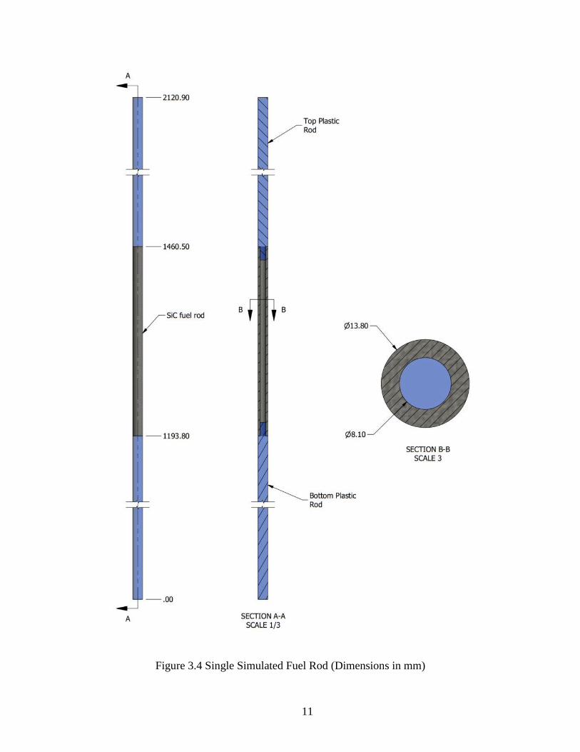
3.2.1 Single Simulated Fuel Rod

The single simulated fuel rod has three major parts: the top plastic rod, the middle

test rod section, and the bottom plastic rod. The single simulated fuel rod is designed such

that all the parts components are assembled in line and joined together to form a single rod.

The top plastic rod is 648 mm in length and has outer diameter of 13.8 mm. The

test rod (SiC fuel rod) is 266.7 mm in length and has an inner diameter of 8.1 mm and an

outer diameter of 13.8 mm. This test rod is attached to the top and bottom plastic rods by

press fittings. The bottom plastic rod of 1168.4 mm length and 13.8 mm outer diameter

serves the purpose of: supporting the middle test rod section and holding it to the desired

elevation from the inlet tee.

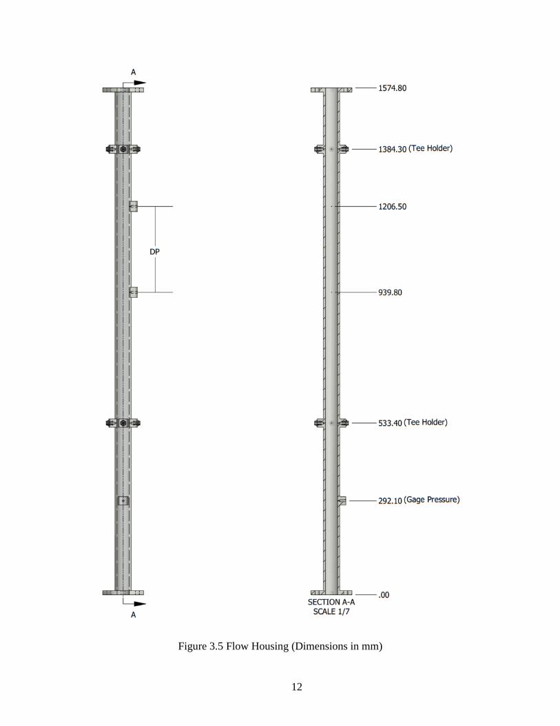
3.2.2 Flow Housing

The flow housing provides the appropriate cross section to accommodate the single

simulated fuel rod at its center. It has two (2) components: (1) the flow shroud tube and (2)

two sets of rod support for ensuring proper alignment.

10

Figure 3.3 Test Section

11

Figure 3.4 Single Simulated Fuel Rod (Dimensions in mm)

12

Figure 3.5 Flow Housing (Dimensions in mm)

13

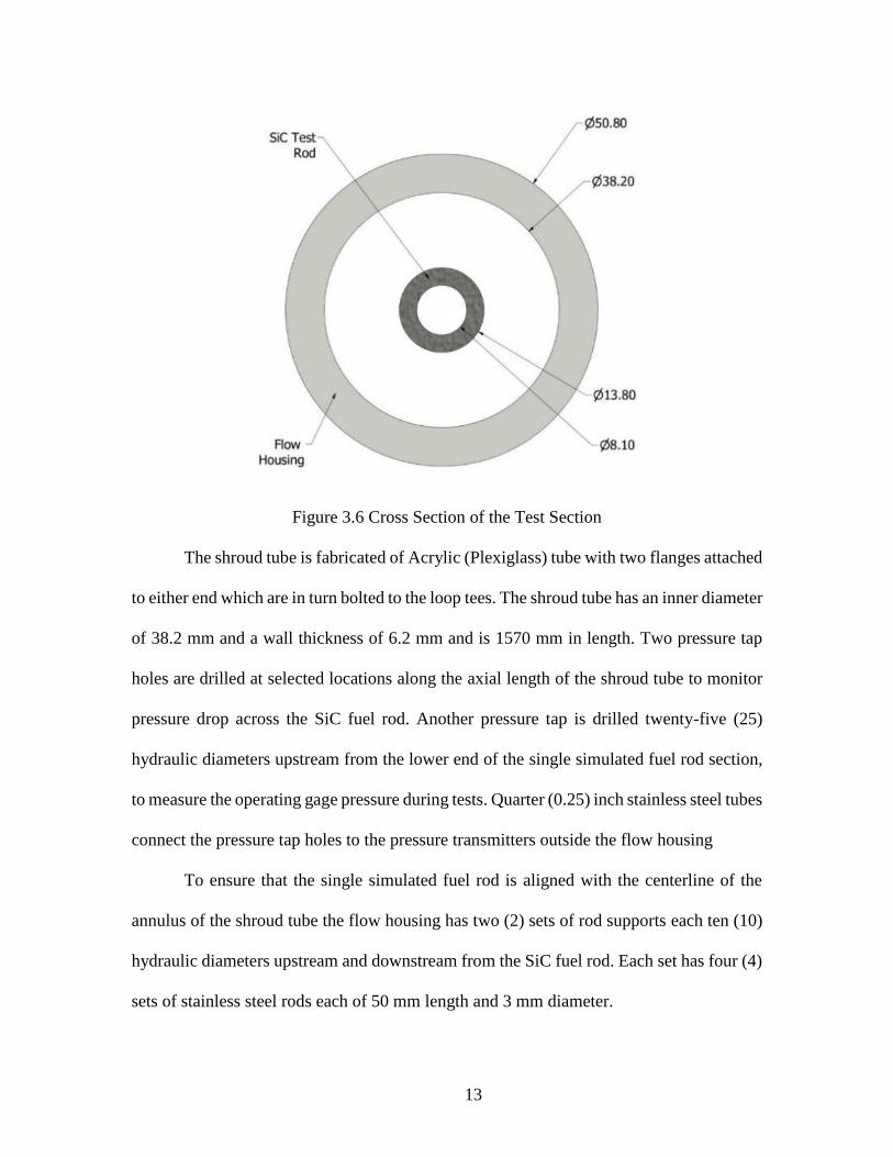
Figure 3.6 Cross Section of the Test Section

The shroud tube is fabricated of Acrylic (Plexiglass) tube with two flanges attached

to either end which are in turn bolted to the loop tees. The shroud tube has an inner diameter

of 38.2 mm and a wall thickness of 6.2 mm and is 1570 mm in length. Two pressure tap

holes are drilled at selected locations along the axial length of the shroud tube to monitor

pressure drop across the SiC fuel rod. Another pressure tap is drilled twenty-five (25)

hydraulic diameters upstream from the lower end of the single simulated fuel rod section,

to measure the operating gage pressure during tests. Quarter (0.25) inch stainless steel tubes

connect the pressure tap holes to the pressure transmitters outside the flow housing

To ensure that the single simulated fuel rod is aligned with the centerline of the

annulus of the shroud tube the flow housing has two (2) sets of rod supports each ten (10)

hydraulic diameters upstream and downstream from the SiC fuel rod. Each set has four (4)

sets of stainless steel rods each of 50 mm length and 3 mm diameter.

14

3.3 Silicon Carbide Fuel Rod

The SiC fuel rod used for the investigation was provided by Westinghouse. The

relatively thin wall tubes fabricated for this work are constructed of 2 layers; an inner thin

wall SiC monolith tube surrounded by SiCf/SiC CMC. The inner thin wall monolith tube

is used to obtain reasonable inner diameter dimensional tolerance for a nuclear fuel

cladding tube and a hermetic seal [2]. The outer SiCf/SiC CMC is used to provide strength

and some amount of durability to a fully ceramic tube. Tubes were designed to have

adequate mechanical properties for normal reactor operating conditions and a design basis

accident, and to withstand impact during handling of a SiCf/SiC CMC tube filled with

uranium dioxide (UO2) fuel pellets. The roughness on the fuel rod was produced by

braiding SiC fiber over the thin wall SiC monolith tubes, depositing a thin pyrolytic carbon

(C) layer onto the braided fiber, and chemical vapor infiltration (CVI) of SiC into and on

the braided fiber. Thus, the surface roughness design on the SiC fuel rod is irregular. The

SiC fuel rod is shown in Figure 3.7. The roughness produced on the SiC tube is irregular.

The roughness height was measured by the “Basic Bench Contour Projector” (shown in

Figure 3.8) at USC. The height of the roughness was measured every 2.667 mm along the

entire length (266.7 mm) of the SiC rod. A total of 100 readings were taken over the 266.7

mm length of the rod. Then the rod was rotated by an angle of 180 degrees and another set

of 100 height readings were measured in a comparable manner. The contour plots obtained

is shown in Figure 3.9. The average height of roughness of the rod is found to be 0.06155

mm and the root mean square of all the values is 0.07629 mm.

15

Figure 3.7 Roughness structure on the SiC Fuel Rod

(a)

(b)

Figure 3.8 (a) Basic Bench Contour Projector used for roughness measurement, (b)

Display of the basic Bench Contour Projector

16

Figure 3.9 Contour plot for the SiC fuel rod surface

3.4 Test Fluid

The test fluid is deionized (DI) water for the following requirements:

Chlorides: less than 0.2 ppm

Solids: less than 0.5 ppm

Oxygen: less than 0.1 ppm

pH: 6.5 to 7.5

Resistivity: 0.5 MΩ/cm (min.)

3.5 Pump

The pump is a 0.75 HP Grundfos model CRIE 10-1 unit, which is a vertical inline

multi-stage booster pump with all wetted parts constructed from 304 series stainless steel,

with a flow capacity of 15 m3/h against a 10 m head. The pump is fitted with cool-top air-

cooled shaft seal chamber and can handle water up to 180˚C.

0

0.05

0.1

0.15

0.2

0.25

0.3

0 50 100 150 200 250 300

Roughnes

s hei

ght,

mm

Length along the length of tube, mm

Contour Plot 1

Contour Plot 2

17

3.6 Flow Meters

The loop includes three flow meters, two to measure the total flow rate through the

test section at lower and higher flow ranges, and the third to measure the flow rate of the

cooling water through the heat exchanger. The system flow meters are Cameron model

NUFLOTM 10 and 38 mm stainless steel turbine meters for lower (0.068-0.68 m3/h) and

higher (3.41-40.88 m3/h) ranges, respectively, with magnetic pickups and silver soldered

shaft and bearings to accommodate temperatures and pressures up to 230˚C and 1.3 MPa,

respectively. The NUFLOTM meter is connected to the data acquisition system. It includes

an analyzer model MC-II Flow mounted directly on the flow meter for flow rate readings.

3.7 Heat Exchangers

After an hour or so of operation the water temperature in the loop rises due to

viscous heating, even when no heat is applied to the simulated fuel rod. When the heated

water exits the test section, it flows through the loop piping and then through the heat

exchanger for cooling to the desired inlet temperature. The heat exchanger is a single-pass

76 mm diameter unit with the shell and the tube sides constructed from 316 stainless steel

and heat transfer area of 1 m2.

3.8 Compressor

A column of air, pressurized by a 0.026 m3/0.9 MPa compressor, sets the system

pressure. The pressurizer is constructed from 304 stainless steel piping partially filled with

water above the loop.

18

3.9 Valves

The SHELT loop bypass and test section valves are 38 mm 316L stainless steel ball

valves that control the water flow rate in the loop. One is located at the exit of the flow rate

control bypass; one is located at the test section inlet temperature control bypass; and the

other at the exit of the test section. A 19-mm precision valve made of brass controls the

water flow rate at the exit of the heat exchanger.

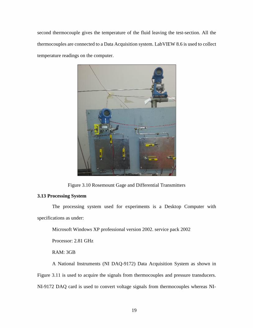
3.10 Gage Pressure Transmitter

The gage pressure in the Loop is monitored at the bottom of the test section by a

Rosemount 2051CG gage pressure transmitter (Figure 3.10). The 4-20 mA current output

from the transmitter is calibrated between 0-2.07 MPa pressures and it can withstand

temperatures of up to 150˚C. The transmitter has a LCD screen display and it is also

connected to the data acquisition system.

3.11 Differential Pressure Transmitter

A Rosemount 2051CD pressure transmitter measures the axial flow resistance

across the SiC fuel rod (Figure 3.10). The 4-20 mA current output from the pressure

transmitter is calibrated between pressures of 0-4.2 KPa. Just like the gage pressure

transmitter the differential pressure transmitter also has a LCD display and its outputs are

also connected to the data acquisition system.

3.12 Thermocouples

Two OMEGA thermocouples (K-types) are inserted in the pipe through press

fittings, the tips of the probe thermocouple are maintained in the middle of the pipe. First

thermocouple gives the temperature reading of DI water going into the test section and the

19

second thermocouple gives the temperature of the fluid leaving the test-section. All the

thermocouples are connected to a Data Acquisition system. LabVIEW 8.6 is used to collect

temperature readings on the computer.

Figure 3.10 Rosemount Gage and Differential Transmitters

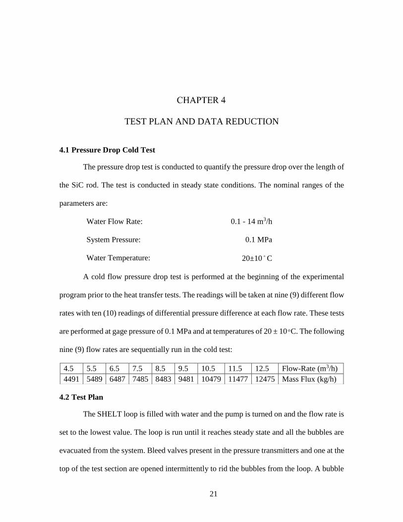
3.13 Processing System

The processing system used for experiments is a Desktop Computer with

specifications as under:

Microsoft Windows XP professional version 2002. service pack 2002

Processor: 2.81 GHz

RAM: 3GB

A National Instruments (NI DAQ-9172) Data Acquisition System as shown in

Figure 3.11 is used to acquire the signals from thermocouples and pressure transducers.

NI-9172 DAQ card is used to convert voltage signals from thermocouples whereas NI-

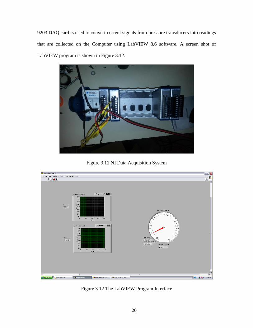
20

9203 DAQ card is used to convert current signals from pressure transducers into readings

that are collected on the Computer using LabVIEW 8.6 software. A screen shot of

LabVIEW program is shown in Figure 3.12.

Figure 3.11 NI Data Acquisition System

Figure 3.12 The LabVIEW Program Interface

21

TEST PLAN AND DATA REDUCTION

4.1 Pressure Drop Cold Test

The pressure drop test is conducted to quantify the pressure drop over the length of

the SiC rod. The test is conducted in steady state conditions. The nominal ranges of the

parameters are:

Water Flow Rate: 0.1 - 14 m3/h

System Pressure: 0.1 MPa

Water Temperature: 20±10˚C

A cold flow pressure drop test is performed at the beginning of the experimental

program prior to the heat transfer tests. The readings will be taken at nine (9) different flow

rates with ten (10) readings of differential pressure difference at each flow rate. These tests

are performed at gage pressure of 0.1 MPa and at temperatures of 20 ± 10 C. The following

nine (9) flow rates are sequentially run in the cold test:

4.2 Test Plan

The SHELT loop is filled with water and the pump is turned on and the flow rate is

set to the lowest value. The loop is run until it reaches steady state and all the bubbles are

evacuated from the system. Bleed valves present in the pressure transmitters and one at the

top of the test section are opened intermittently to rid the bubbles from the loop. A bubble

4.5 5.5 6.5 7.5 8.5 9.5 10.5 11.5 12.5 Flow-Rate (m3/h)

4491 5489 6487 7485 8483 9481 10479 11477 12475 Mass Flux (kg/h)

22

free system is confirmed by looking closely at the test section through the transparent

Plexiglas flow housing. Temperatures at the inlet and outlet of the test section are

monitored by two K-type thermocouples, which are connected to the LabVIEW computer

through the NI DAQ. The loop is considered to have reached steady state when the

temperature readings of the inlet and outlet do not vary by more than 0.5˚C over a period

of 20 minutes. Once steady state is achieved the reading of pressure drop are collected from

the differential pressure transmitters. The same procedure is repeated by increasing the

flow rate, and thus the readings for all nine flow rates are collected.

4.3 Control Test

Before testing the Silicon Carbide nuclear fuel rod a control test was carried out by

using a fuel rod of similar dimensions to that of the SiC rod. This was done for dual

purpose: first to compare the present results with those of previous experiments, thereby

ensuring that the experimental setup is working correctly, and secondly to establish a

reference for the results obtained with rough tubes. Similar strategies were employed by

previous investigators [15]. This test is repeated 3 times to ensure repeatability of results.

4.4 Data Reduction

The flow rate (Q) was measured from the flow meters. The mean velocity was

measured from the flow rate and the cross sectional area of the annulus of the test section

𝑈𝑚 =𝑄

𝐴𝑐 4.1

Where, 𝐴𝑐 = 𝜋(𝑟𝑜2 − 𝑟𝑖

2)

The Reynolds Number was calculated as follows:

23

𝑅𝑒 =𝑈𝑚𝐷ℎ

𝜗 4.2

Where, 𝐷ℎ = 2(𝑟𝑜 − 𝑟𝑖) and 𝜗 is the kinematic viscosity of the fluid.

The equation for friction factor is given as follows:

𝑓 = −2 (

𝛥𝑝𝛥𝑥)𝐷ℎ

𝜌𝑈𝑚2 4.3

Where, 𝛥𝑝

𝛥𝑥 is the pressure drop per unit length.

The friction factor obtained from the correlation [16] in equation 4.4 is compared

with the experimental friction factor obtained for the smooth rod.

𝑓 = 0.184𝑅𝑒−1/5 4.4

Dimensions of the simulated Smooth and Rough Rods

Type of Rod Diameter in m Length in m

Smooth Rod 0.013758 0.2667

Rough SiC Rod 0.0135636 0.2667

For calculation purposes the following values were used:

𝜌 = 995.03 kg/m3

𝜗 = 0.801*10-6 m2s-1

4.5 Test Parameter Tolerance

Actual test conditions must meet the requirements provided in Section 4.1 within

the following limits:

Water Flow Rate: ±0.07 m3/h

System Pressure: ±1.55 KPa

Water Temperature: ±0.24 ˚C

24

4.6 Uncertainty Analysis

The experimental uncertainty was calculated using the Kline McClintock formula.

This is given as:

𝑈𝑓 = √(𝜕𝑓

𝜕∆𝑝)2

𝑈∆𝑝2 + (

𝜕𝑓

𝜕𝑄)2

𝑈𝑄2 4.5

where 𝑈∆𝑝 is given as

𝑈∆𝑝 = √(𝑈𝑎𝑐𝑐𝑢𝑟𝑎𝑐𝑦)2+ (𝑈𝑟𝑎𝑛𝑑𝑜𝑚)2 4.6

where, 𝑈𝑎𝑐𝑐𝑢𝑟𝑎𝑐𝑦 is the uncertainty due to bias error of the instrumentation and 𝑈𝑟𝑎𝑛𝑑𝑜𝑚

is the uncertainty due to the randomness of the obtained readings. The uncertainty for the

investigation was found to be ±1.67%.

25

CFD ANALYSIS

In this chapter, details will be provided on the development of a the CFD model. A

2D CFD model of the flow was created in ANSYS Fluent. The Fluent solver is based on

the Finite Volume Method. The purpose of the CFD model is to: 1) Compare and validate

the experimental results of friction factor for the SiC roughness design, 2) To numerically

ascertain the heat transfer enhancement, 3) Get some insights into the flow mechanism that

is involved which increases the heat transfer and pressure drop.

5.1 Flow Domain

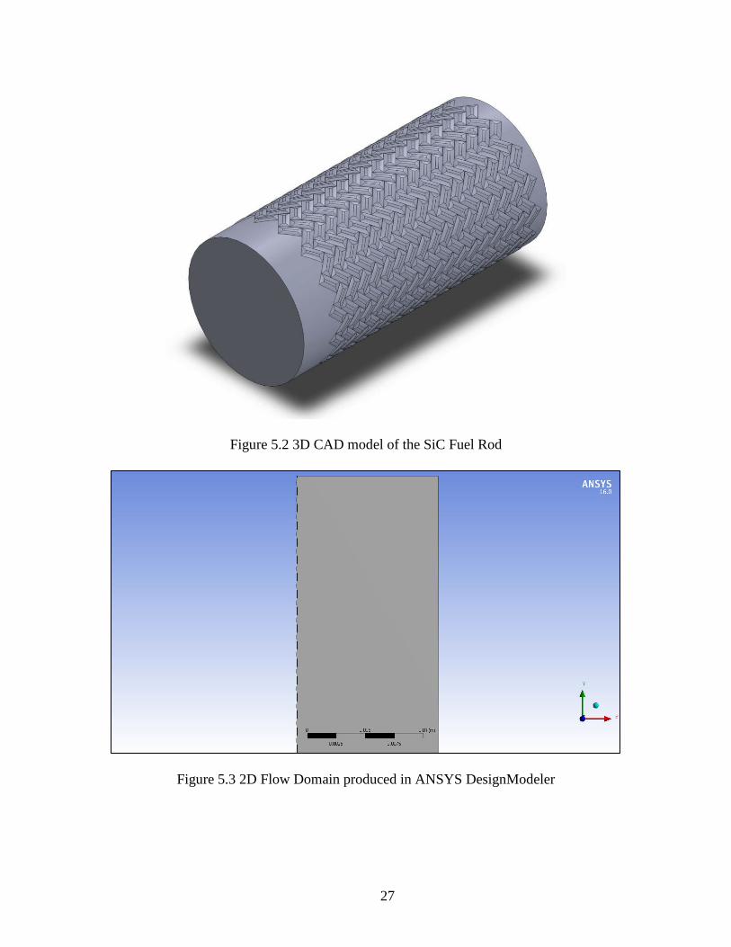
The flow domain created for the CFD analysis is shown in Figure 5.1. A 3D CAD

model (Figure 5.2) of the SiC Fuel rod was created in SolidWorks. This model was

imported into the ANSYS workbench DesignModeler. The model was then modified to

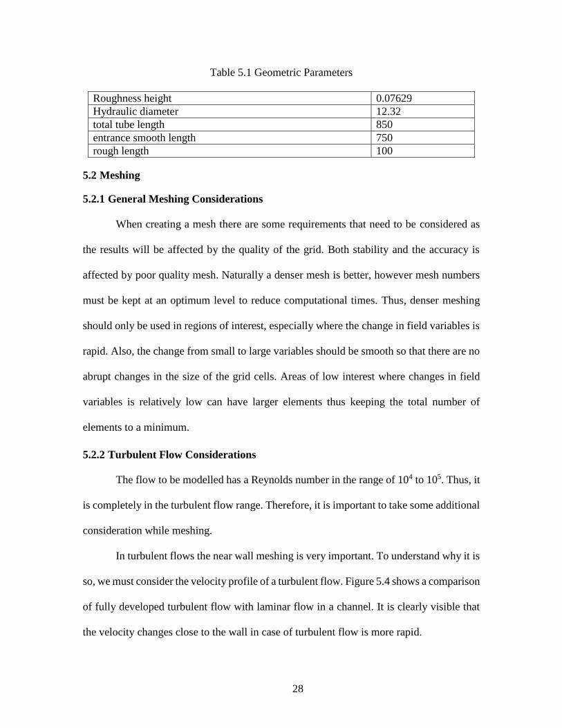
achieve the 2D flow domain as shown in Figure 5.2. The geometric design parameters for

the rod are given in Table 5.1. It is to be noted that the geometric model of the roughness

design created had some inherent errors. The actual SiC fuel rod was produced by vapor

deposition and braiding, thus it had irregular bumps and very fine thread like features on

its surface. These were difficult to measure thus they were ignored in the CAD design. So,

the CAD model created for the roughness design was less rough than the actual SiC fuel

rod. Thus, we expect the CFD results to give a lower approximation of the friction factor

when compared to the experimental results.

26

Figure 5.1 Flow Domain used for CFD Analysis

CFD Model Flow Domain

(Not Drawn to

Scale)

Start of Rough

wall

0.74 m

0.85 m

Detail C

27

Figure 5.2 3D CAD model of the SiC Fuel Rod

Figure 5.3 2D Flow Domain produced in ANSYS DesignModeler

28

Table 5.1 Geometric Parameters

Roughness height 0.07629

Hydraulic diameter 12.32

total tube length 850

entrance smooth length 750

rough length 100

5.2 Meshing

5.2.1 General Meshing Considerations

When creating a mesh there are some requirements that need to be considered as

the results will be affected by the quality of the grid. Both stability and the accuracy is

affected by poor quality mesh. Naturally a denser mesh is better, however mesh numbers

must be kept at an optimum level to reduce computational times. Thus, denser meshing

should only be used in regions of interest, especially where the change in field variables is

rapid. Also, the change from small to large variables should be smooth so that there are no

abrupt changes in the size of the grid cells. Areas of low interest where changes in field

variables is relatively low can have larger elements thus keeping the total number of

elements to a minimum.

5.2.2 Turbulent Flow Considerations

The flow to be modelled has a Reynolds number in the range of 104 to 105. Thus, it

is completely in the turbulent flow range. Therefore, it is important to take some additional

consideration while meshing.

In turbulent flows the near wall meshing is very important. To understand why it is

so, we must consider the velocity profile of a turbulent flow. Figure 5.4 shows a comparison

of fully developed turbulent flow with laminar flow in a channel. It is clearly visible that

the velocity changes close to the wall in case of turbulent flow is more rapid.

29

Figure 5.5 Experimental Turbulent boundary layer profiles for various

pressure gradients [17]

Figure 5.4 Comparison of fully developed laminar and turbulent flow in channel [17]

30

Figure 5.5 shows experimental Turbulent boundary layer profiles for various

pressure gradients. If we consider the graph for the strong favorable gradient it appears as

if there is velocity slip in the wall. But there is no velocity slip. The velocity profile actually

changes very rapidly to zero in a thickness that is very small (0 ≤ y/δ < 0.002). A better

understanding of the boundary layer can be obtained by referring to Figure 5.6.

Figure 5.6 Subdivision of Near Wall Region[18]

Here the near wall region has been divided into subdivisions by introducing two

new parameters (non-dimensional distance from the wall, y+; the wall friction velocity, uτ).

The viscous sublayer near the wall which extends from y+ values 0 to 5 is a region where

viscous shear dominates. In the outer layer the Turbulent shear has the dominating effect.

31

Figure 5.7 Near wall meshing approaches[18]

The meshing in the viscous sublayer is vital for getting accurate results in case of

turbulent flows. There are two approaches for the near wall meshing (Figure 5.7):

1. Wall Function Approach: This does not solve the governing equations in the near

wall region but uses functions. Thus, the near wall meshing need not be very fine.

2. Near-Wall Model Approach: In this approach, the near wall region is resolved

by solving the governing equations. Thus, the mesh in that region needs to be

very fine, and y+~1 needs to be achieved. This was the approach that was taken

for this CFD analysis.

5.2.3 Mesh Calculations

Calculations are needed to be performed to find the position of the first node (∆y)

from the wall. To do this, first the friction factor value is needed to be assumed. For the

smooth rod this was assumed by equation 4.4:

32

𝑓 = 0.184𝑅𝑒−1/5 4.4

For the rough rod the equation proposed by Haaland [19] for sand grain roughness

was used to assume the friction factor:

𝑓−1/2 = −1.8𝑙𝑜𝑔 (6.9

𝑅𝑒+ (

𝑘𝑠/𝐷ℎ

3.7)1.11

) 5.1

Where 𝐷ℎ is the Hydraulic Diameter and 𝑘𝑠 is the sand grain roughness height

(taken as 0.07629 mm). For both the smooth and the rough SiC rod the following

calculations are performed to obtain the position of the first node of the mesh from the wall

to satisfy the y+ requirements.

𝐶𝑓 = 0.25𝑓 5.2

𝜏𝑤 = 0.5𝐶𝑓𝜌𝑈𝑚2 5.3

𝑈𝜏 = (𝜏𝑤

𝜌)0.5 5.4

𝛥𝑦 =𝑦+𝜗

𝑈𝜏 5.5

Where for water at 30˚C,

ρ = 995.03 kg/m3, ϑ = 8.01e-7 m2s-1

Both triangular and quadrilateral elements were used in order to mesh the flow

domain. The near wall region of the wall was meshed by using the inflation option in the

ANSYS Workbench Meshing. The area in the free stream of the domain was meshed by

using triangular elements. At first a coarse mesh was used. This mesh was improved and

made finer until mesh independence was achieved. Mesh independence study was made

by comparing 4 mesh models with 1530233, 1932818, 3011863 and 3908981 elements.

33

Table 5.2 Meshing Parameters

near wall

first layer thickness 0.0023

number of inflation layers 32

growth rate 1.1

y+ covered 0.6 ~ 120

freestream region

maximum face size 0.1

minimum face size 0.0006

-875

-870

-865

-860

-855

-850

-845

-840

10 15 20 25 30 35 40P

ress

ure

Dro

p p

er U

nit

len

gth

(P

a/m

)

Number of Elements (x105)

Mesh Convergence

achieved

Figure 5.8 Grid Independence study

Mesh Model 1

Mesh Model 2 Mesh Model 3

Mesh Model 4

34

Figure 5.9 Meshing in rough region

Figure 5.10 Mesh in the transition region between smooth and rough rod

Figure 5.11 Meshing in smooth Region

Rough Rod Region

Transition region between

smooth and rough rod

Smooth Rod Region

35

As seen in Figure 5.8 the Pressure drop per unit length between the Model 1 and

Model 2 increased by 3%. For Mesh Model No. 2 and 3 the Pressure Drop per unit length

is almost the same. Therefore, the mesh independence is achieved at Mesh Model No. 2.

This is further confirmed since after mesh model no. 4 with 3908981 elements we see that

the Pressure Drop per unit length decreases. Figure 5.9 to Figure 5.11 shows the mesh

model used for one of the flow rates.

5.3 Numerical Methods

5.3.1 Governing Equations

This section will introduce the governing equations used to solve the fluid flow and

heat transfer inside the computational domain. The flow field solutions are obtained by

solving the time averaged continuity and momentum equations in 2D. The time averaged

energy equation is solved to obtain the heat transfer analysis.

The steady state continuity equation which expresses the conservation of mass for

an incompressible fluid is defined as:

𝜵 ∙ �� = 0 5.6

The Reynolds Averaged Navier Stokes (RANS) equation is as:

𝜌𝐷��

𝐷𝑡= 𝜌𝑔 − 𝛻�� + ∇ ∙ 𝜏𝑖𝑗 5.7

Where,

𝜏𝑖𝑗 = 𝜇 (𝜕𝑢𝑖

𝜕𝑥𝑗+

𝜕𝑢𝑗

𝜕𝑥𝑖) − 𝜌𝑢′𝑖𝑢′𝑗

The Energy Equation is expressed as:

𝜌𝐶𝑃

𝐷��

𝐷𝑡= −

𝜕

𝜕𝑥𝑗(𝑞𝑖) + ∅ 5.8

36

Where,

∅ =𝜇

2(𝜕𝑢��

𝜕𝑥𝑗+

𝜕𝑢𝑖′

𝜕𝑥𝑗+

𝜕𝑢��

𝜕𝑥𝑖+

𝜕𝑢𝑖′

𝜕𝑥𝑗)

2

𝑞𝑖 = −𝑘𝜕��

𝜕𝑥𝑖+ 𝜌𝐶𝑃𝑢𝑖

′𝑇′

It is to be noted that the time averaging of the Navier Stokes equations introduced

new unknowns into the flow equations through the 𝜏𝑖𝑗 term. Thus, new equations needs to

be solved to find the new unknowns.

The procedure of solving the new unknowns is known as turbulence modeling.

There are a number of turbulence models, and one of them is called the k-ω shear stress

transport (SST) model [20], [21], which is used in this analysis. This model uses the

advantages of both the k-ε and the k-ω models. The k-ω model is more accurate near the

wall layers, and has been successful with flows with moderate adverse pressure gradients.

However, the ω equation shows sensitivity to the values of ω in the freestream outside the

boundary layer [22]. The k-ε model is more accurate in the freestream region away from

the wall. The SST model divides the flow domain into two regions, and it uses blending

functions to switch between k-ε and k-ω models. The k-ω SST model is also a better choice

when compared with the wall functions since it solves the flow equations near the walls,

and thus reveals flow characteristics in the near wall region. One of the drawbacks of using

SST model is that it requires a very fine mesh in the laminar sublayer region extending up

to the buffer layer. This requirement significantly increases the computation effort. Hence,

this analysis uses a dense and structured mesh for near wall regions.

37

5.3.2 Solution Procedures

The Fluent solver is used to solve the governing equations by using a steady state

Pressure-based solver. The pressure based solver uses an algorithm where the mass

conservation of the velocity field is achieved by solving a pressure equation. The pressure

equation is derived from the continuity and momentum equations so that the velocity field

corrected by the pressure satisfies continuity. The governing equations are nonlinear and

coupled to one another. Thus, a solution is obtained by iteration of the complete set of

governing equations until convergence is obtained.

A step by step solution strategy was employed for the computational analysis. The

flow equations (continuity and RANS) do not have any temperature terms, thus they can

be solved to convergence at first. Then the heat equation is turned on and all the equations

are solved to convergence.

The Boundary Conditions (BC) were set as shown in Figure 5.12. The inlet BC was

set as velocity inlet, and a temperature of 303 K was set. A constant heat flux of 232509

W/m2 was set at the inner wall. A turbulent intensity of 5% and turbulent length scale of

Dh was set at the inlet to calculate the initial guess values of k and ω. The solution methods

were set up as shown in Figure 5.13.

To simulate the experimental results correctly a fully developed flow must be

established before flow hits the rough section. To ensure this numerically a line was plotted

vertically along the center of the flow domain. The velocity was plotted along this line as

shown in Figure 5.14. The velocity initially increases as y increases and then it remains

constant until the flow hits the rough section. Fully developed conditions are achieved at

the point shown in the Figure 5.14.

38

Figure 5.12 Boundary Conditions

Figure 5.13 Finite Difference Schemes used for discretization of the various terms in the

governing equations

Pressure Outlet

Velocity Inlet (I=5%, Dh)

Inner wall

No Slip BC

q′′=232509

W/m2

Smooth wall

No Slip BC

Constant T

39

Figure 5.14 Velocity vs. y (elevation) drawn along center of flow domain

Figure 5.15 Locations where pressure drops are measured

3.5

3.6

3.7

3.8

3.9

4

4.1

4.2

0 0.1 0.2 0.3 0.4 0.5 0.6 0.7 0.8

Vel

oci

ty i

n m

/s

y in m

RoughSmooth

fully developed

flow from here

∆pr

∆ps

40

5.4 Data Reduction

5.4.1 Friction Factor Calculations

The friction factor results from CFD for the smooth section was compared with the

correlation in equation 4.4.

The CFD results for the friction factor in the smooth and rough section is calculated

using the following formula:

𝑓 = −2 (

𝛥𝑝𝛥𝑥)𝐷ℎ

𝜌𝑈𝑚2 5.9

5.4.2 Heat Transfer enhancement calculations

For the computation of the heat transfer enhancement for the smooth section the

following calculations were performed:

𝑇𝑏1=

1

𝐷ℎ∫ 𝑇(𝑥) ⅆ𝑥

𝐷ℎ

0

5.10

ℎ =𝑞′′

(𝑇𝑤 − 𝑇𝑏1) 5.11

𝑁𝑢 =ℎ𝐷ℎ

𝑘𝑓 5.12

Where 𝑇𝑏1and 𝑇𝑤were measured at the locations shown in Figure 5.16.

The heat transfer enhancement for the smooth section were compared with the

Gnelinksi Correlation [23]:

𝑁𝑢 =

[ ((

𝑓8) (𝑅𝑒 − 1000)𝑃𝑟)

1 + 12.7 (𝑓8)

12𝑃𝑟

23 − 1]

5.13

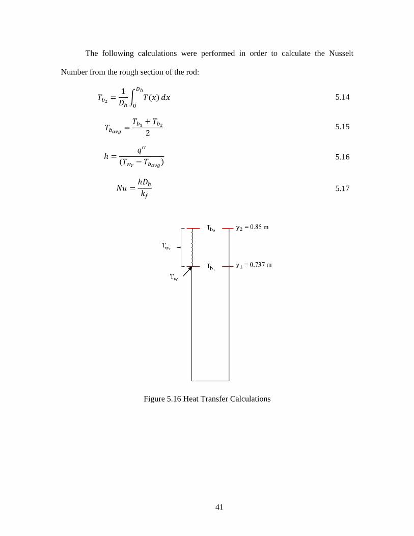
41

The following calculations were performed in order to calculate the Nusselt

Number from the rough section of the rod:

𝑇𝑏2=

1

𝐷ℎ∫ 𝑇(𝑥) ⅆ𝑥

𝐷ℎ

0

5.14

𝑇𝑏𝑎𝑣𝑔=

𝑇𝑏1+ 𝑇𝑏2

2 5.15

ℎ =𝑞′′

(𝑇𝑤𝑟− 𝑇𝑏𝑎𝑣𝑔

) 5.16

𝑁𝑢 =ℎ𝐷ℎ

𝑘𝑓 5.17

Figure 5.16 Heat Transfer Calculations

42

RESULTS

6.1 Experimental Results

6.1.1 Pressure Drop Results for Smooth Rod

The loop was first run with the smooth rod. The data for pressure drop were

collected over the nine different flow rates. In total four sets of results were collected to

ensure repeatability of the results as outlined in section 4.1. All data were collected at

temperatures and pressures of 30˚C and 0.05 MPa, respectively.

These data obtained from the experiment were then compared with the Correlation

in equation 4.4. In Figure 6.1 friction factor is plotted as a function of the Reynolds number,

and the experimental data for smooth rod from the three test runs are compared with that

from correlation. The maximum recorded deviation between the experimental results and

the correlation is ±2.36%. Taking into consideration the calculated uncertainty for the

obtained value of friction factor, we can safely conclude that the experimental values agree

well with the correlation. Looking at the graph we can also conclude that it passes the

repeatability criteria.

6.1.2 Pressure Drop Results for Rough Rod

The pressure drop results for the SiC rough rod are shown in Figure 6.2. The

obtained points for friction factor pass the repeatability tests and shows that friction factor

drops as Reynolds number increases, as was the case with the smooth rod. However, the

43

rate of fall of friction factor with increase in Reynolds Number is lower when compared

with that of the smooth rod. At the lowest investigated Reynolds No. of 40,000 a friction

factor increase of 7.6 % is observed and at the highest Reynolds No. of 110,000 the friction

factor increase was 15%, when compared with the smooth rod.

6.2 Numerical Results

6.2.1 Validation of the numerical model

Validation of the CFD model developed in ANSYS Fluent was done by comparing

the CFD results for friction factor of the smooth section with that obtained from correlation

in equation 4.4. Figure 6.3 plots the friction factor for the smooth section obtained from

the CFD model compared to that obtained from the Correlation. The CFD results for the

friction factor for smooth section shows a maximum deviation of ±4% from the correlation.

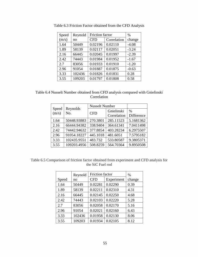
Figure 6.4 shows the results of friction factor for the SiC roughness design obtained

from the experiments and from the CFD model. It is clearly noticed that the CFD analysis

gives a lower estimation of the friction factor. This was expected for reasons explained in

section 5.1. The maximum deviation from the experimental results is 8%, which occurs at

the highest Reynolds Number.

Figure 6.5 shows the results for the Nusselt Number from CFD analysis and from

the Gnielinski Correlation. It is observed that the Nusselt number increases when the Re

No. increases which is due to the viscous sublayer becoming thinner. The viscous sublayer

can act as an obstruction to the heat transfer from the hot fuel rod walls. Results for Nusslelt

Number are also found to lie very close to those suggested by Gnielinksi Correlation. A

maximum deviation of 9.9% is recorded.

44

From these results we can safely conclude that the CFD model is validated and thus

can be used to compute the expected heat transfer enhancement that can be achieved by the

SiC roughness design.

6.2.2 Numerical Results of Heat Transfer enhancement for SiC roughness design

Figure 6.6 and Figure 6.7, shows the flow characteristics around the roughness

structures. Figure 6.6 shows the streamlines and the pressure contour plots for the case with

Reynolds number 102436. From the figure recirculation zones/boundary layer separation

is clearly identified. Adverse pressure gradients exist at points where recirculation is

identified. Adverse pressure gradient is a necessary condition for flow separation. Flow

separation occurs when the adverse pressure gradient along with the shear from the wall

creates enough opposing resistance to the flow, to overcome the forward momentum of the

fluid particles and cause them to flow in reverse direction. It is interesting to note that at a

small distance away from the roughness structures towards the freestream, the streamlines

become almost parallel and the roughness has no effect on the flow. The total resistance on

the roughened surface is made up of the pressure forces and the skin-friction forces. The

skin friction depends on the wall shear stress distribution. The pressure forces depend on

the size of the wake formed beyond the separation point. The wake is a low-pressure region

and a bigger wake formation results in a higher pressure drag.

Figure 6.7 shows the isotherms and the streamlines near a typical roughness

element. It is found that the temperature of the water near the recirculation region is the

highest and attains maximum near the point where separation begins. The temperature of

water near the reattachment point is lower. Thus, near reattachment points the heat transfer

from the wall to the water is the highest. Figure 6.8 shows the wall temperature variations

45

along the rough fuel rod wall. It is seen that in the smooth section the wall temperature

increases slowly but in the rough region the wall temperature is fluctuating rapidly. Thus

in order to find the actual overall heat transfer enhancement the average is to be found for

the entire roughened region of the SiC rod.

The results for Nusselt number are obtained from the CFD model for six values of

Reynolds number in the range 5x104 to 1.1x105. For each Reynolds Number investigated

the Nusselt Number is measured using the calculations as outlined in section 5.4.2.

Figure 6.9 shows the comparisons of Nusselt Number for the smooth and the rough

rods. It is observed that the Nusselt number for the rough rod is always greater than that

obtained for the smooth rod. A maximum heat transfer enhancement of 18.4% can be

achieved with the rough rod at the highest Reynolds Number investigated. The surface

roughness structures in the fuel rod promotes turbulence which enhances heat transfer by

breaking the thermal boundary layer and stimulating turbulent mixing. However, we can

expect that in actual practical application the roughness design will provide a heat transfer

enhancement greater than 18.4% for reasons explained in section 5.1.

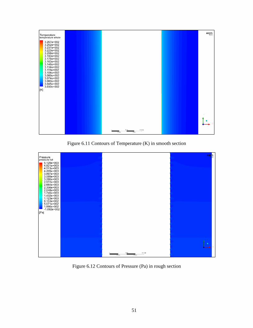
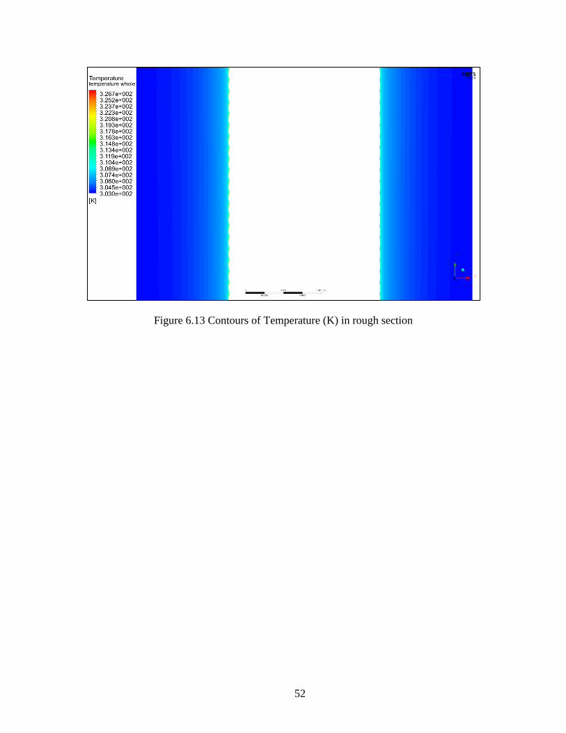
Figure 6.10 to Figure 6.13 shows the contour plots of Pressures and Temperatures

in the rough and smooth sections

46

Figure 6.2 Comparison of experimental results of friction factor for SiC rod with the

smooth rod.

0.017

0.018

0.019

0.02

0.021

0.022

0.023

40000 50000 60000 70000 80000 90000 100000 110000

Fri

ctio

n F

acto

r, f

Reynolds Number, Re

Set 1

Set 2

Set3

Correlation

0.017

0.018

0.019

0.02

0.021

0.022

0.023

0.024

40000 50000 60000 70000 80000 90000 100000 110000

Fri

ctio

n F

acto

r, f

Reynolds Number, Re

Set 1 Set 2 Set 3 Set 1 Set 2 Set 3Rough: Smooth:

Figure 6.1 Comparison of Smooth Friction factor results from experiment with

correlation

47

Figure 6.3 Comparison of friction factor for smooth rod from CFD analysis and

Correlation

Figure 6.4 Comparison of friction factor obtained from Experiment and CFD analysis

0.017

0.018

0.019

0.020

0.021

0.022

0.023

4 6 8 10

Fri

ctio

n F

acto

r, f

Reynolds Number, Re (x104)

CFD smooth section

Correlation

0.017

0.018

0.019

0.02

0.021

0.022

0.023

0.024

4 6 8 10

Fri

ctio

n f

acto

r, f

Reynolds Number, Re (x104)

CFD Experimental

48

Figure 6.5 Comparison of Nusselt No. at the smooth section (y1=0.737 m) from CFD

analysis and Gnielinski Correlation.

Figure 6.6 Pressure contours and streamlines around roughness

structures (Re=102,436)

250

300

350

400

450

500

550

600

45000 55000 65000 75000 85000 95000 105000 115000

Nu

ssel

t N

o., N

u

Reynolds No.

CFD Smooth

Boundary layer

Separation

49

Figure 6.7 Temperature contours and streamlines around roughness structures

(Re=102,436)

Figure 6.8 Wall Temperature variation Twr along the rough wall

314

316

318

320

322

324

326

328

0.7 0.72 0.74 0.76 0.78

Wal

l T

emp

erat

ure

in

K

Length in m

Smooth Rough

50

Figure 6.9 Comparison of Nusselt Number from CFD analysis for smooth

and rough rods

Figure 6.10 Contours of Pressure (Pa) in smooth section

0

100

200

300

400

500

600

700

45000 55000 65000 75000 85000 95000 105000 115000

Nu

ssel

t N

o., N

u

Reynolds No.

CFD Smooth

CFD Rough

51

Figure 6.11 Contours of Temperature (K) in smooth section

Figure 6.12 Contours of Pressure (Pa) in rough section

52

Figure 6.13 Contours of Temperature (K) in rough section

53

Table 6.1 Results for friction factor for smooth rods

Data

Set

Flow

Rate

(m3/hr)

Um

in m/s

Reynold's

No.

Pressure

drop

(mmHg)

Pressure

Drop

(Pascal)

friction

factor

friction

factor

(theoretical)

1

4.831 1.345 41054 1.586 211.49 0.02152 0.02199

5.923 1.650 50334 2.335 311.32 0.02108 0.02111

6.789 1.891 57694 2.998 399.66 0.02059 0.02054

7.798 2.172 66268 3.860 514.58 0.02010 0.01998

8.715 2.427 74061 4.736 631.43 0.01975 0.01954

9.725 2.708 82644 5.781 770.68 0.01935 0.01912

10.652 2.967 90522 6.762 901.54 0.01887 0.01877

11.981 3.337 101816 8.508 1134.23 0.01877 0.01833

12.713 3.541 108037 9.418 1255.61 0.01845 0.01812

2

4.831 1.346 41075 1.596 212.83 0.02164 0.02198

5.913 1.648 50275 2.327 310.24 0.02105 0.02111

6.778 1.889 57629 3.005 400.61 0.02069 0.02054

7.798 2.173 66302 3.869 515.86 0.02013 0.01998

8.726 2.431 74192 4.760 634.58 0.01977 0.01953

9.735 2.713 82771 5.740 765.24 0.01916 0.01911

10.652 2.968 90567 6.738 898.28 0.01878 0.01877

11.991 3.341 101952 8.363 1115.01 0.01840 0.01833

12.723 3.545 108176 9.330 1243.90 0.01823 0.01811

3

4.821 1.343 40970 1.607 214.28 0.02190 0.02200

5.954 1.658 50598 2.370 316.02 0.02117 0.02109

6.768 1.885 57515 2.992 398.90 0.02068 0.02055

7.757 2.160 65920 3.843 512.36 0.02022 0.02000

8.767 2.442 74503 4.782 637.53 0.01970 0.01952

9.735 2.711 82729 5.802 773.47 0.01938 0.01911

10.652 2.967 90522 6.828 910.31 0.01905 0.01877

11.960 3.331 101638 8.420 1122.54 0.01864 0.01834

12.774 3.558 108555 9.457 1260.80 0.01835 0.01810

54

Table 6.2 Friction Factor results with the rough SiC rod

Data

Set

Flow Rate

(m3/hr)

Um

(m/s)

Reynold's

No.

Presure Drop

(mmHg)

Pressure Drop

(Pa)

friction

factor

1

4.842 1.343 41301 1.692 225.57 0.02316

5.913 1.640 50437 2.495 332.59 0.02289

6.82 1.891 58174 3.347 446.20 0.02309

7.798 2.163 66516 4.267 568.81 0.02251

8.726 2.420 74431 5.274 703.11 0.02222

9.745 2.703 83123 6.433 857.62 0.02174

10.662 2.957 90945 7.661 1021.31 0.02162

12.002 3.329 102375 9.542 1272.12 0.02125

12.805 3.551 109225 10.759 1434.34 0.02105

2

4.852 1.346 41387 1.716 228.74 0.02338

5.903 1.637 50352 2.467 328.93 0.02272

6.799 1.886 57994 3.298 439.63 0.02289

7.798 2.163 66516 4.229 563.86 0.02232

8.705 2.414 74252 5.218 695.64 0.02209

9.756 2.706 83217 6.498 866.34 0.02191

10.662 2.957 90945 7.656 1020.68 0.02161

11.991 3.326 102281 9.556 1273.99 0.02133

12.795 3.548 109139 10.766 1435.26 0.02110

3

4.821 1.337 41122 1.696 226.13 0.02342

5.975 1.657 50966 2.580 343.95 0.02319

6.758 1.874 57645 3.246 432.80 0.02281

7.726 2.143 65902 4.193 559.06 0.02254

8.756 2.428 74687 5.369 715.78 0.02247

9.735 2.700 83038 6.522 869.52 0.02208

10.621 2.946 90595 7.660 1021.25 0.02179

11.96 3.317 102017 9.565 1275.22 0.02146

12.774 3.543 108960 10.835 1444.54 0.02131

55

Table 6.3 Friction Factor obtained from the CFD Analysis

Speed

(m/s)

Reynold

no

Friction factor %

change CFD Correlation

1.64 50449 0.02196 0.02110 -4.08

1.89 58139 0.02117 0.02051 -3.24

2.16 66445 0.02045 0.01997 -2.39

2.42 74443 0.01984 0.01952 -1.67

2.7 83056 0.01933 0.01910 -1.20

2.96 91054 0.01887 0.01875 -0.63

3.33 102436 0.01826 0.01831 0.28

3.55 109203 0.01797 0.01808 0.58

Table 6.4 Nusselt Number obtained from CFD analysis compared with Gnielinski

Correlation

Speed

(m/s)

Reynolds

No.

Nusselt Number

CFD Gnielinski

Correlation

%

Difference

1.64 50448.93883 270.3801 285.11523 5.1681362

2.16 66444.94382 338.9404 364.61341 7.0411498

2.42 74442.94632 377.8854 403.28234 6.2975507

2.96 91054.18227 445.1018 481.6051 7.5795182

3.33 102435.9551 483.732 533.80587 9.3805371

3.55 109203.4956 508.8259 564.70364 9.8950508

Table 6.5 Comparison of friction factor obtained from experiment and CFD analysis for

the SiC Fuel rod

Speed

Reynold

no

Friction factor %

change CFD Experiment

1.64 50449 0.02281 0.02290 0.39

1.89 58139 0.02211 0.02310 4.31

2.16 66445 0.02145 0.02250 4.68

2.42 74443 0.02103 0.02220 5.28

2.7 83056 0.02058 0.02170 5.16

2.96 91054 0.02021 0.02160 6.43

3.33 102436 0.01958 0.02130 8.06

3.55 109203 0.01934 0.02105 8.12

56

Table 6.6 Nusselt Number calculations for the SiC rod

Speed (m/s) Tb1 Tb2 Tbavg

T𝑤𝑟 h Nu rough

1.64 305.291 305.775 305.533 338.57667 7036.416 278.4998

2.16 304.733 305.091 304.912 329.96415 9281.001 367.7831

2.42 304.536 304.536 304.536 325.90759 10879.35 431.309

2.96 304.254 304.254 304.254 321.8536 13211.04 524.0686

3.33 304.121 304.356 304.2385 320.36791 14415.22 572.0122

3.55 304.052 304.275 304.1635 319.48336 15176.96 602.3264

Table 6.7 % increasein Nusselt Number

Reynolds

Number

CFD Analysis % increase in

Nusselt

Number Smooth Rough

50449 270.38 278.50 3.00

66445 338.94 367.78 8.51

74443 377.89 431.31 14.14

91054 445.10 524.07 17.74

102436 483.73 572.01 18.25

109203 508.83 602.33 18.38

57

CONCLUSION AND FUTURE RESEARCH

7.1 Conclusion

The objective of the research outlined in this thesis was to experimentally determine

the friction factor of a simulated Silicon Carbide (SiC) nuclear fuel rod, with three

dimensional surface roughnesses which was produced by vapor deposition and braiding of

SiC fibres. The experimental results were compared with correlations and with

experimental results from a smooth rod. The Single Heater Element Loop tester (SHELT)

at USC was used to conduct the experimental testing. The experimental results were

validated by checking with correlations, and then confirming repeatability of the results.

The experimental results indicates that the roughness design on the SiC fuel rod will

increase the flow resistance by 15% at the highest Reynolds number studied.

A Computational model was also established to study the friction factor and heat

transfer enhancements for the SiC nuclear fuel rod. The roughness design on the SiC rod

was modeled by using SolidWorks. The CFD model was established by using the ANSYS

Fluent solver, which used Finite Difference Methods in order to solve the governing

equations. The CFD model for the SiC fuel rod was validated by comparing with

experimental results. The friction factor results obtained from the CFD results vary from

the experimental results with a maximum deviation of 8%. This was considered to lie

58

within reasonable limits considering the inherent errors associated with the CAD design of

the SiC roughness design. The thermal results obtained from the CFD analysis suggested

that the roughness design will enhance heat transfer by at least 18.4% at the highest

Reynolds number.

7.2 Future Research

In order to validate the thermal CFD model a experimental investigation with heat

transfer should be conducted. This can be achieved by applying heat to the SiC fuel rod

using the Power Supply already available in the SHELT Loop. The rod can be heated by

either using of cartridge heater or by using resistive heating techniques as was done in

previous investigations [13], [14].

59

REFERENCES

[1] L. Meyer, A. Bastron, J. Hofmeister, and T. Schulenberg, “Enhancement of Heat

Transfer in Fuel Assemblies of High Performance Light Water Reactors,” J. Nucl.

Sci. Technol., vol. 44, no. 3, pp. 270–276, 2007.

[2] S. C. Johnson, H. Patts, and D. E. Schuler, “Mechanical Behavior of SiC f / SiC

CMC Tubes Relative to Nuclear Fuel Cladding,” Proc. ICAPP 2014, pp. 2287–

2295, 2014.

[3] T. S. Ravigururajan and A. E. Bergles, “Development and verification of general

correlations for pressure drop and heat transfer in single-phase turbulent flow in

enhanced tubes,” Exp. Therm. Fluid Sci., vol. 13, no. 1, pp. 55–70, 1996.

[4] H. L. Heinisch, L. R. Greenwood, W. J. Weber, and R. E. Williford, “Displacement

damage cross sections for neutron-irradiated silicon carbide,” J. Nucl. Mater., vol.

307–311, no. Part 2, pp. 895–899, 2002.

[5] D. Carpenter, G. Kohse, and M. Kazimi, “Modeling of silicon carbide duplex

cladding designs for high burnup light water reactor fuel,” in International congress

on advances in nuclear power plants, 2007.

[6] D. M. Carpenter, “An assessment of silicon carbide as a cladding material for light

water reactors,” Massachusetts Institute of Technology, 2014.

[7] J. Nikuradse, “Laws of flow in rough pipes,” in National Advisory Committee for

Aeronautics, 1950.

[8] M. E. Steinke and S. G. Kandlikar, “Review of single-phase heat transfer

60

enhancement techniques for application in microchannels, minichannels and

microdevices,” Int. J. Heat Technol., vol. 22, pp. 3–11, 2004.

[9] R. J. Firth and L. Meyer, “A comparison of the heat transfer and friction factor

performance of four different types of artificially roughened surface,” Int. J. Heat

Mass Transf., vol. 26, no. 2, pp. 175–183, 1983.

[10] X. W. Li, J. A. Meng, and Z. X. Li, “Roughness enhanced mechanism for turbulent

convective heat transfer,” Int. J. Heat Mass Transf., vol. 54, no. 9–10, pp. 1775–

1781, 2011.

[11] D. N. Ryu, D. H. Choi, and V. C. Patel, “Analysis of turbulent flow in channels

roughened by two-dimensional ribs and three-dimensional blocks. Part I:

Resistance,” Int. J. Heat Fluid Flow, vol. 28, pp. 1098–1111, 2007.

[12] D. N. Ryu, D. H. Choi, and V. C. Patel, “Analysis of turbulent flow in channels

roughened by two-dimensional ribs and three-dimensional blocks. Part II: Heat

Transfer,” Int. J. Heat Fluid Flow, vol. 28, pp. 1112–1124, 2007.

[13] L. Carrilho, “Experimental and Computational study of roughened surface for PWR

rod bundles,” University of South Carolina, 2012.

[14] U. Najeeb, “Heat Transfer Characteristics of Three-Dimensional Surface Roughness

in Nuclear Fuel Rod Bundles,” in International Mechanical Engineering Congress

& Exposition, 2013.

[15] D. F. Dippery and R. H. Sabersky, “Heat and Momentum Transfer in Smooth and

Rough Tubes at Various Prandtl Numbers,” Int. J. Heat Mass Transf., vol. 6, pp.

328–353, 1963.

[16] F. P. Incropera, D. P. DeWitt, T. L. Bergman, and A. S. Lavine, Fundamentals of

61

Heat and Mass Transfer, 6th Editio. 2006.

[17] F. M. White, Viscous fluid flow, 2nd Editio. 1991.

[18] A. 16.0, “FLUENT Manual,” .

[19] S. E. Haaland, “Simple and Explicitly Formulas for the Friction Factor in Turbulent

Pipe Flow,” J. Fluids Eng., vol. 105, pp. 89–90, 1983.

[20] F. R. Menter, “Zonal two equation k- ω turbulence models for aerodynamic flows,”

AIAA Pap., vol. 2906, 1993.

[21] F. R. Menter, M. L. Suc, and M. Library, “Two-equation eddy-viscosity turbulence

models for engineering applications,” AIAA J., vol. 32, pp. 1598–1605, 1994.

[22] F. R. Menter, “Influence of freestream values on k-w turbulence model predictions,”

AIAA J., vol. 30, pp. 1657–1659, 1992.

[23] V. Gnielinski, “New equations for heat and mass transfer in the turbulent flow in

pipes and channels,” Int. Chem. Eng., vol. 75, pp. 359–368, 1976.