EXPERIMENTAL AND NUMERICAL INVESTIGATION OF … · The prediction of freezing meat inside the cold...
12
http://www.iaeme.com/IJMET/index.asp 213 [email protected] International Journal of Mechanical Engineering and Technology (IJMET) Volume 7, Issue 3, May–June 2016, pp.213–224, Article ID: IJMET_07_03_020 Available online at http://www.iaeme.com/IJMET/issues.asp?JType=IJMET&VType=7&IType=3 Journal Impact Factor (2016): 9.2286 (Calculated by GISI) www.jifactor.com ISSN Print: 0976-6340 and ISSN Online: 0976-6359 © IAEME Publication EXPERIMENTAL AND NUMERICAL INVESTIGATION OF TEMPERATURE DISTRIBUTION FOR MEAT DURING FREEZING PROCESS Husam Mahdi Hadi Sig Combibloc Obeikan, Baghdad, Iraq Qasim S. Mahdi Department of Mechanical Engineering, College of Engineering, Al-Mustansiriyah University, Baghdad, Iraq Nessrian Ali Hussien Department of Chemical Industries, Institute of Technology, Bgahdad, Iraq ABSTRACT The prediction of freezing meat inside the cold storage is studied experimentally and numerically using CFX14.5. In the present work a prototype cold storage for meat has been designed and constructed with dimensions 1 m in length x 1 m in width x 1 m in height. Temperature distributions of regular shape of meats were determined for storage temperature -21°C inside the cold storage, where each part of meat is located in one of the three levels (bottom, medium and top) inside the cold store. The air velocity distribution has been measured by using metal vane anemometer in the directions of (x, -x, y, -y, z and -z) around the meat and the results have been used in the numerical simulations. In the numerical simulations the temperature distributions are based on transient, Navier-Stokes equations, turbulence is taken into account using a standard model for air flow and assumed as steady turbulent state, meats are presented as solid domain with variable thermophysical properties as function of temperature and mass and heat transfer due to evaporation are regulated due to including product casings. During the freezing the properties of meat change during the three stages each stage having specific properties. The minimum temperature of the product was located in the top level and very close to their surrounding storage air temperature both due to exposure to higher air velocity from the fans. The total error of compression between the experimental and numerical temperature distributions of meats is equal to 18.7%.
Transcript of EXPERIMENTAL AND NUMERICAL INVESTIGATION OF … · The prediction of freezing meat inside the cold...

http://www.iaeme.com/IJMET/index.asp 213 [email protected]
International Journal of Mechanical Engineering and Technology (IJMET)
Volume 7, Issue 3, May–June 2016, pp.213–224, Article ID: IJMET_07_03_020
Available online at
http://www.iaeme.com/IJMET/issues.asp?JType=IJMET&VType=7&IType=3
Journal Impact Factor (2016): 9.2286 (Calculated by GISI) www.jifactor.com
ISSN Print: 0976-6340 and ISSN Online: 0976-6359
© IAEME Publication
EXPERIMENTAL AND NUMERICAL
INVESTIGATION OF TEMPERATURE
DISTRIBUTION FOR MEAT DURING
FREEZING PROCESS
Husam Mahdi Hadi
Sig Combibloc Obeikan, Baghdad, Iraq
Qasim S. Mahdi
Department of Mechanical Engineering,
College of Engineering, Al-Mustansiriyah University, Baghdad, Iraq
Nessrian Ali Hussien
Department of Chemical Industries,
Institute of Technology, Bgahdad, Iraq
ABSTRACT
The prediction of freezing meat inside the cold storage is studied
experimentally and numerically using CFX14.5. In the present work a
prototype cold storage for meat has been designed and constructed with
dimensions 1 m in length x 1 m in width x 1 m in height. Temperature
distributions of regular shape of meats were determined for storage
temperature -21°C inside the cold storage, where each part of meat is located
in one of the three levels (bottom, medium and top) inside the cold store. The
air velocity distribution has been measured by using metal vane anemometer
in the directions of (x, -x, y, -y, z and -z) around the meat and the results have
been used in the numerical simulations. In the numerical simulations the
temperature distributions are based on transient, Navier-Stokes equations,
turbulence is taken into account using a standard model for air flow and
assumed as steady turbulent state, meats are presented as solid domain with
variable thermophysical properties as function of temperature and mass and
heat transfer due to evaporation are regulated due to including product
casings. During the freezing the properties of meat change during the three
stages each stage having specific properties. The minimum temperature of the
product was located in the top level and very close to their surrounding
storage air temperature both due to exposure to higher air velocity from the
fans. The total error of compression between the experimental and numerical
temperature distributions of meats is equal to 18.7%.
Husam Mahdi Hadi, Qasim S. Mahdi and Nessrian Ali Hussien
http://www.iaeme.com/IJMET/index.asp 214 [email protected]
Key words: Cold Store; CFD Model; Simulation; Air Flow; Temperature
Distribution; Meat; Thermo-Phyical Properties; Food Industry.
Cite this Article: Husam Mahdi Hadi, Qasim S. Mahdi and Nessrian Ali
Hussien, Experimental and Numerical Investigation of Temperature
Distribution For Meat During Freezing Process. International Journal of
Mechanical Engineering and Technology, 7(3), 2016, pp. 213–224.
http://www.iaeme.com/currentissue.asp?JType=IJMET&VType=7&IType=3
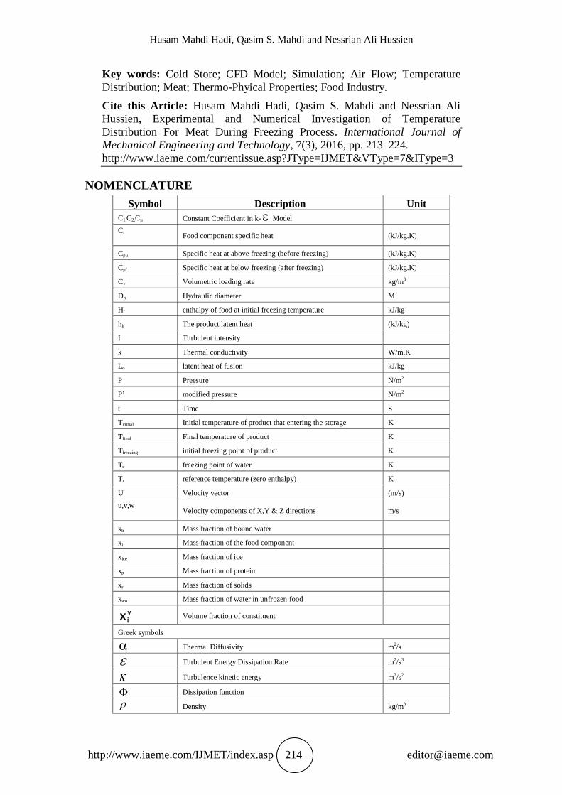
NOMENCLATURE
Symbol Description Unit
C1,C2,Cµ
Constant Coefficient in k- Model
Ci
Food component specific heat (kJ/kg.K)
Cpu Specific heat at above freezing (before freezing) (kJ/kg.K)
Cpf Specific heat at below freezing (after freezing) (kJ/kg.K)
Cv Volumetric loading rate kg/m3
Dh Hydraulic diameter M
Hf enthalpy of food at initial freezing temperature kJ/kg
hif The product latent heat (kJ/kg)
I Turbulent intensity
k Thermal conductivity W/m.K
Lo latent heat of fusion kJ/kg
P Preesure N/m2
P’
modified pressure N/m2
t Time S
Tinitial Initial temperature of product that entering the storage K
Tfinal Final temperature of product K
Tfreezing initial freezing point of product K
To freezing point of water K
Tr reference temperature (zero enthalpy) K
U Velocity vector (m/s)
u,v,w
Velocity components of X,Y & Z directions m/s
xb Mass fraction of bound water
xi Mass fraction of the food component
xice Mass fraction of ice
xp Mass fraction of protein
xs Mass fraction of solids
xwo Mass fraction of water in unfrozen food
νix
Volume fraction of constituent
Greek symbols
Thermal Diffusivity m2/s
Turbulent Energy Dissipation Rate m2/s3
Turbulence kinetic energy m2/s2
Dissipation function
Density kg/m3

Experimental and Numerical Investigation of Temperature Distribution For Meat During
Freezing Process
http://www.iaeme.com/IJMET/index.asp 215 [email protected]
Symbol Description Unit
i density of the food constituents kg/m3
Dynamic Viscosity N.s/m2
eff Effective viscosity (kg/m.s)
T
Turbulent viscosity (kg/m.s)
second viscosity (kg/ms)
k , Empirical Constant
1. INTRODUCTION
Food freezing, which is a process used to minimize physical, biochemical and
microbiological changes in food, is of great importance in the food industry. This
preservative effect is maintained by subsequent storage of the frozen food at a
sufficiently cold temperature. The freezing process for foods with high water content,
between 50% and 95%, is divided into three stages; the first is precooling stage. This
involves cooling down from the initial temperature of the product to the product
without effecting phase change, and is referred to as sensible heat. The second is
phase change stage; this stage covers the formation of ice in the products and extends
from the initial freezing point to a medium temperature about 5°C colder at the center
of the product. The third is tempering stage; this is a cooling-down period to the
ultimate temperature for storage and begins when the contribution of the latent heat is
negligible compared to that of the sensible heat. The frozen product has a non-
uniform temperature distribution: warmer in the center and coldest at the surfaces. Its
average temperature corresponds to the value reached when the temperature of the
product is allowed to equilibrate. In general, it is recommended that the product be
cooled in the freezer to an equilibrium temperature of -18°C or colder [1].
There are several studies on the experimental and numerical investigation of
temperature distribution in food industry:
Pierre Sylvain Mirade et al. 2002, [2], studied three dimensional CFD calculations
for designing large food chillers. The CFD code Fluent/UNS was used to simulate the
airflow patterns inside the chiller. This procedure was applied to a pork chiller
containing 290 carcasses. Two design cases differing in inlet air direction and flow
rate, and two functioning modes, batch and continuous were analyzed. Experimentally
the carcasses arranged in in six rows (47 in rows 1 and 6, and 49 in the other rows).
For the continuous chiller analysis the mean, center and surface temperature kinetics
calculated for a carcass weight of 80 kg, where the average velocity is 0.17 m/s,
Surface temperature is always about 15 °C lower than the mean temperature and
storage temperature -10°C. Numerical result were made to determine the air velocity
and air temperature inside a batch chiller the results show the average is 0.2m/sec and
0°C respectively. the results show that a further 8 hr are needed to reach a mean
temperature of 7°C at the core and the total chilling time of 13hr changing from first
ventilation level to the second reduces the chilling time by only 20 min, while
increasing the total weight loss from 1.3 to 1.7%. Jihan, 2010, [3] Studied the heat
transfer during cooling for irregular shaped meat and poultry products. Numerically a
three-dimensional finite element algorithm implemented in Java was used to solve the
model. Model validation was conducted using data collected in four different meat
processing facilities, under real time varying processing conditions. The model was
adapted to receive input parameters that are readily available and can easily be

Husam Mahdi Hadi, Qasim S. Mahdi and Nessrian Ali Hussien
http://www.iaeme.com/IJMET/index.asp 216 [email protected]
provided by meat processors such as air relative humidity, air temperature, air
velocity, type of casing, duration of water shower, and product weight and core
temperature prior to entering the chiller. Gong Jianying et al. 2010, [4] a three
dimensional mathematical model is established to study the flow field distribution and
radish temperature distribution inside a cold store. The result shows the flow field is
very non-uniform distribution is harmful to cold storage effect and the storage
product. Seyed Majid et al. 20012, [5] presented a numerical model to predict air
flow, heat and mass transfer in order to evaluate the cooling performance of a typical
full loaded cold storage using CFD code fluent 6.1. Apples are packed in the vented
containers of 30 kg weight. The results showed the temperature difference between
5.5°C and 9.5°C between the hottest and coolest product’s temperature during the
cooling time. Also, the results shows the errors of about 23.2% between the
experimental and numerical, and 9.1% were achieved for velocity magnitude
prediction in the cool storage and the product weight loss after 54 days of cooling in
the loaded cool storage, respectively. The objectives of the present paper are to
investigate experimentally and numerically temperature distribution of meats that
distributed in three levels inside the cold store during freezing process for air storage
temperature below -20°C.
2. MATHEMATICAL MODELING
2.1. Physical model and thermo-physical properties of meat:
The dimensions of the simulated meat are (18cm × 11cm × 3cm) distributed in three
levels inside the cold storage. Type of meat used in the present work are Indian cut
meat with the moisture content and its composition (see table (1)) are taken from
Babji, 1989 [6]. The thermo- physical properties (such as thermal conductivity,
specific heat, enthalpy and density) of meat are calculated from empirical relations
ASHRAE, 1998, [7]. The essential equations for thermo- physical properties of meat
as the following:
)8(
)7(
)6()(])(
26.155.1[)(
)5()()628.03.219.4)((
)4(
)3(/
1
)2(4.0
)1(1
3
ii
iii
ii
initialr
freezingbwo
srinitial
ssfreezinginitialf
iip
ii
pb
initial
f
bwoice
x
xx
kxk
meatfrozenforTT
TLxxxTTH
meatunfrozenforxxTTHH
xcc
x
xx
T
Txxx
Experimental and Numerical Investigation of Temperature Distribution For Meat During
Freezing Process
http://www.iaeme.com/IJMET/index.asp 217 [email protected]
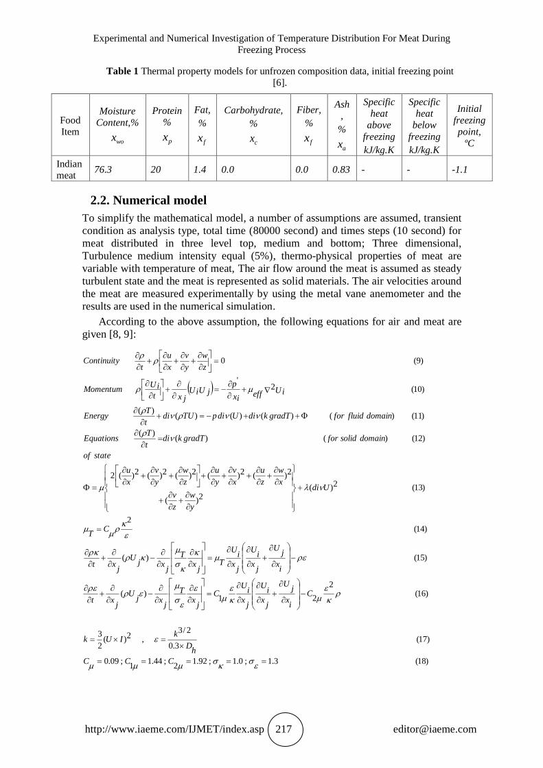
Table 1 Thermal property models for unfrozen composition data, initial freezing point
[6].
Food
Item
Moisture
Content,%
wox
Protein
%
px
Fat,
%
fx
Carbohydrate,
%
cx
Fiber,
%
fx
Ash
,
%
ax
Specific
heat
above
freezing
kJ/kg.K
Specific
heat
below
freezing
kJ/kg.K
Initial
freezing
point,
ºC
Indian
meat 76.3 20 1.4 0.0 0.0 0.83 - - -1.1
2.2. Numerical model
To simplify the mathematical model, a number of assumptions are assumed, transient
condition as analysis type, total time (80000 second) and times steps (10 second) for
meat distributed in three level top, medium and bottom; Three dimensional,
Turbulence medium intensity equal (5%), thermo-physical properties of meat are
variable with temperature of meat, The air flow around the meat is assumed as steady
turbulent state and the meat is represented as solid materials. The air velocities around
the meat are measured experimentally by using the metal vane anemometer and the
results are used in the numerical simulation.
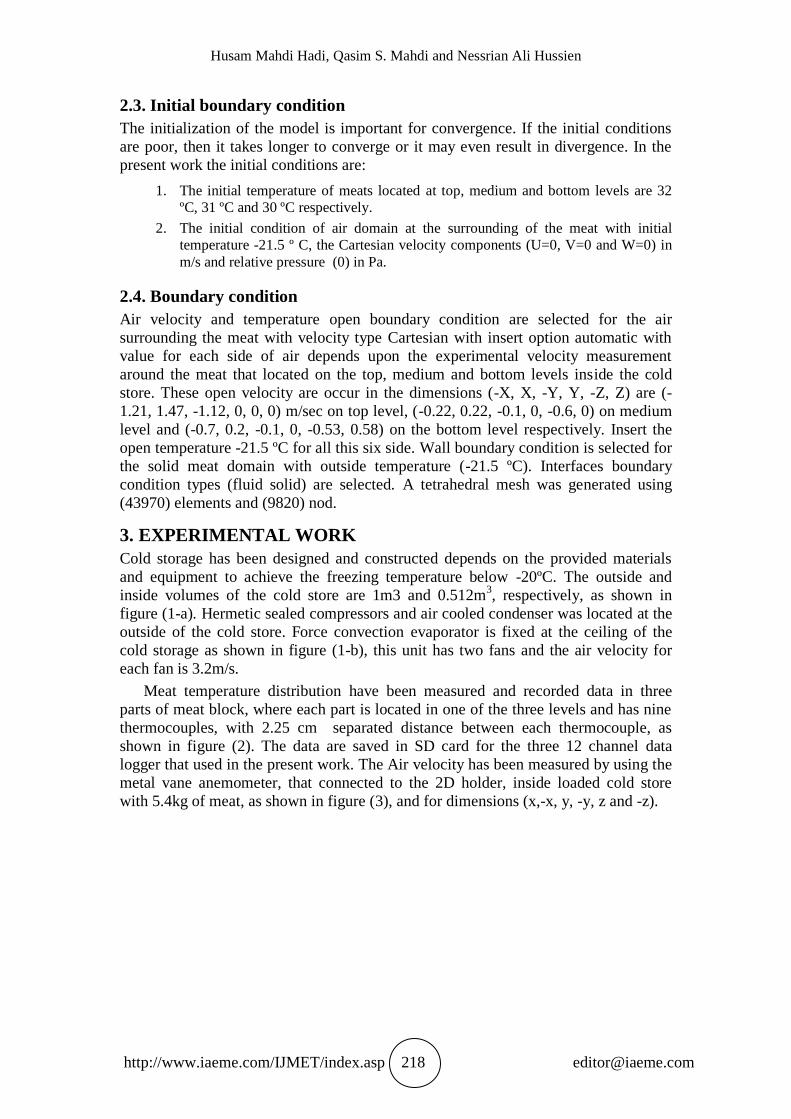
According to the above assumption, the following equations for air and meat are
given [8, 9]:
)18(3.1;0.1;92.12
;44.11
;09.0
)17(3.0
2/3,2)(
2
3
)16(2
21)(
)15()(
)14(2
)13(2)(2)(
2)(2)(2)(2)(2)(2
)12()()()(
)11()()()()()(
)10(2'
)9(0
CCC
hD
kIUk
C
ix
jU
jx
iU
jx
iU
C
jx
T
jxj
U
jxt
ix
jU
jx
iU
jx
iU
Tj
xT
jxj
U
jxt
CT
Udi
y
w
z
v
x
w
z
u
x
v
y
u
z
w
y
v
x
u
stateof
domainsolidforgradTkdit
TEquations
domainfluidforgradTkdiUdipTUdit
TEnergy
Uieffxi
pU jUi
x jt
UiMomentum
z
w
y
v
x
u
tContinuity
Husam Mahdi Hadi, Qasim S. Mahdi and Nessrian Ali Hussien
http://www.iaeme.com/IJMET/index.asp 218 [email protected]
2.3. Initial boundary condition
The initialization of the model is important for convergence. If the initial conditions
are poor, then it takes longer to converge or it may even result in divergence. In the
present work the initial conditions are:
1. The initial temperature of meats located at top, medium and bottom levels are 32
ºC, 31 ºC and 30 ºC respectively.
2. The initial condition of air domain at the surrounding of the meat with initial
temperature -21.5 º C, the Cartesian velocity components (U=0, V=0 and W=0) in
m/s and relative pressure (0) in Pa.
2.4. Boundary condition
Air velocity and temperature open boundary condition are selected for the air
surrounding the meat with velocity type Cartesian with insert option automatic with
value for each side of air depends upon the experimental velocity measurement
around the meat that located on the top, medium and bottom levels inside the cold
store. These open velocity are occur in the dimensions (-X, X, -Y, Y, -Z, Z) are (-
1.21, 1.47, -1.12, 0, 0, 0) m/sec on top level, (-0.22, 0.22, -0.1, 0, -0.6, 0) on medium
level and (-0.7, 0.2, -0.1, 0, -0.53, 0.58) on the bottom level respectively. Insert the
open temperature -21.5 ºC for all this six side. Wall boundary condition is selected for
the solid meat domain with outside temperature (-21.5 ºC). Interfaces boundary
condition types (fluid solid) are selected. A tetrahedral mesh was generated using
(43970) elements and (9820) nod.
3. EXPERIMENTAL WORK
Cold storage has been designed and constructed depends on the provided materials
and equipment to achieve the freezing temperature below -20ºC. The outside and
inside volumes of the cold store are 1m3 and 0.512m3, respectively, as shown in
figure (1-a). Hermetic sealed compressors and air cooled condenser was located at the
outside of the cold store. Force convection evaporator is fixed at the ceiling of the
cold storage as shown in figure (1-b), this unit has two fans and the air velocity for
each fan is 3.2m/s.
Meat temperature distribution have been measured and recorded data in three
parts of meat block, where each part is located in one of the three levels and has nine
thermocouples, with 2.25 cm separated distance between each thermocouple, as
shown in figure (2). The data are saved in SD card for the three 12 channel data
logger that used in the present work. The Air velocity has been measured by using the
metal vane anemometer, that connected to the 2D holder, inside loaded cold store
with 5.4kg of meat, as shown in figure (3), and for dimensions (x,-x, y, -y, z and -z).

Experimental and Numerical Investigation of Temperature Distribution For Meat During
Freezing Process
http://www.iaeme.com/IJMET/index.asp 219 [email protected]
(a) (b)
Figure 1 (a) The cold storage and (b) The evaporator and fans (inside unit).
Figure 2 Thermocouples distribution to measure meat temperature at three levels
Figure 3 Measurement of air velocity around the meat using metal vane anemometer.
4. RESULTS AND DISCUSSION
4.1. Experimental results
Temperature distribution inside meat has been measured along the z-direction, where
the distance between one of the thermocouple and another is 2.25 cm. The initial
temperatures of the meat at the top, medium and bottom levels were 32°C, 31°C and
30°C respectively. Since meat is frozen from the outside and then toward the center, it
is impossible to judge by the outward appearance or the feel of the meat whether the
whole of it is frozen. The surface of the meat, which is close to the freezing medium,
will very quickly be reduced to a temperature near that of the freezer. The temperature
inside the meat will, however, change more slowly. Since the freezing time of a
product is taken for the warmest point of the meat to reach a desired temperature, it is
Husam Mahdi Hadi, Qasim S. Mahdi and Nessrian Ali Hussien
http://www.iaeme.com/IJMET/index.asp 220 [email protected]
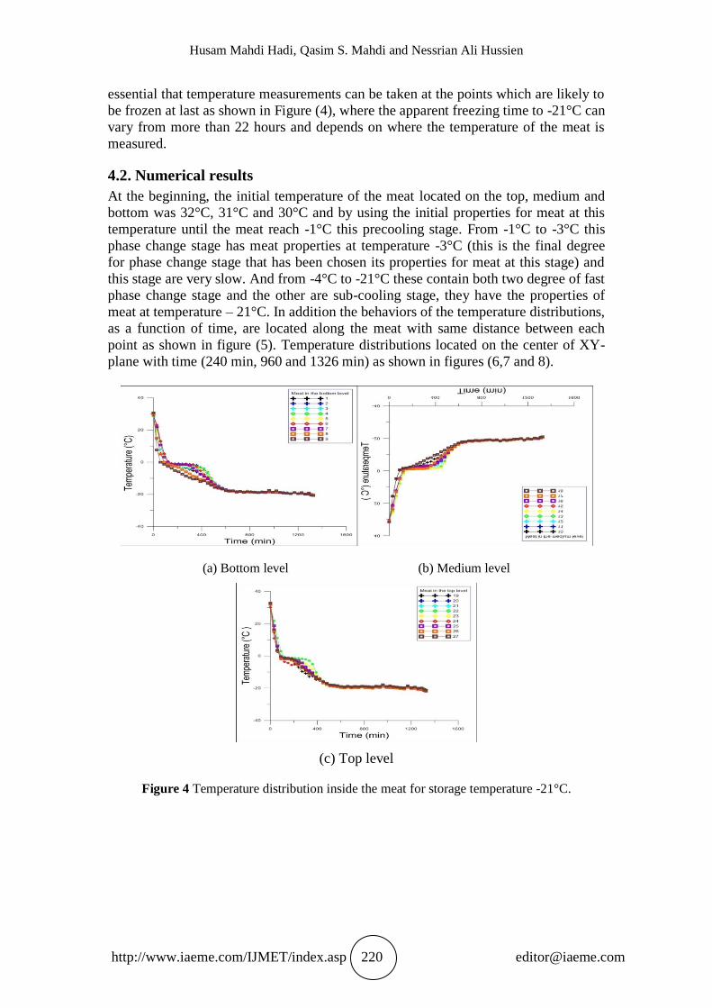
essential that temperature measurements can be taken at the points which are likely to
be frozen at last as shown in Figure (4), where the apparent freezing time to -21°C can
vary from more than 22 hours and depends on where the temperature of the meat is
measured.
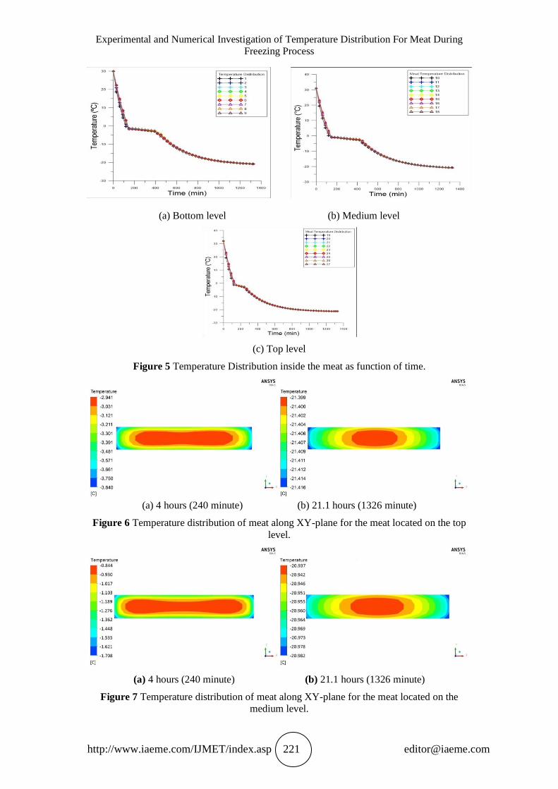
4.2. Numerical results
At the beginning, the initial temperature of the meat located on the top, medium and
bottom was 32°C, 31°C and 30°C and by using the initial properties for meat at this
temperature until the meat reach -1°C this precooling stage. From -1°C to -3°C this
phase change stage has meat properties at temperature -3°C (this is the final degree
for phase change stage that has been chosen its properties for meat at this stage) and
this stage are very slow. And from -4°C to -21°C these contain both two degree of fast
phase change stage and the other are sub-cooling stage, they have the properties of
meat at temperature – 21°C. In addition the behaviors of the temperature distributions,
as a function of time, are located along the meat with same distance between each
point as shown in figure (5). Temperature distributions located on the center of XY-
plane with time (240 min, 960 and 1326 min) as shown in figures (6,7 and 8).
(a) Bottom level (b) Medium level
(c) Top level
Figure 4 Temperature distribution inside the meat for storage temperature -21°C.
Experimental and Numerical Investigation of Temperature Distribution For Meat During
Freezing Process
http://www.iaeme.com/IJMET/index.asp 221 [email protected]
(a) Bottom level (b) Medium level
(c) Top level
Figure 5 Temperature Distribution inside the meat as function of time.
(a) 4 hours (240 minute) (b) 21.1 hours (1326 minute)
Figure 6 Temperature distribution of meat along XY-plane for the meat located on the top
level.
(a) 4 hours (240 minute) (b) 21.1 hours (1326 minute)
Figure 7 Temperature distribution of meat along XY-plane for the meat located on the
medium level.
Husam Mahdi Hadi, Qasim S. Mahdi and Nessrian Ali Hussien
http://www.iaeme.com/IJMET/index.asp 222 [email protected]
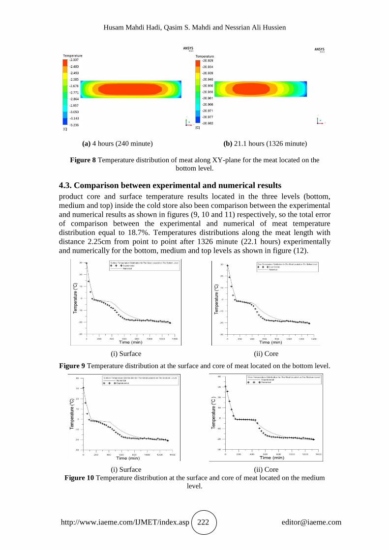
(a) 4 hours (240 minute) (b) 21.1 hours (1326 minute)
Figure 8 Temperature distribution of meat along XY-plane for the meat located on the
bottom level.
4.3. Comparison between experimental and numerical results
product core and surface temperature results located in the three levels (bottom,
medium and top) inside the cold store also been comparison between the experimental
and numerical results as shown in figures (9, 10 and 11) respectively, so the total error
of comparison between the experimental and numerical of meat temperature
distribution equal to 18.7%. Temperatures distributions along the meat length with
distance 2.25cm from point to point after 1326 minute (22.1 hours) experimentally
and numerically for the bottom, medium and top levels as shown in figure (12).
(i) Surface (ii) Core
Figure 9 Temperature distribution at the surface and core of meat located on the bottom level.
(i) Surface (ii) Core
Figure 10 Temperature distribution at the surface and core of meat located on the medium
level.

Experimental and Numerical Investigation of Temperature Distribution For Meat During
Freezing Process
http://www.iaeme.com/IJMET/index.asp 223 [email protected]
(i) Surface (ii) Core
Figure 11 Temperature distribution of the surface and core of meat located on the top level.
(i) Bottom level (ii) Medium level
(iii) Top level
Figure 12 Comparison between experimental and numerical for meat temperature distribution
with length after 1326 minute for meat located at three levels.

Husam Mahdi Hadi, Qasim S. Mahdi and Nessrian Ali Hussien
http://www.iaeme.com/IJMET/index.asp 224 [email protected]
5. CONCLUSIONS
From the present work results for the temperature distribution of meat inside the cold
store, different distinguish conclusions have been pointed out:
1. The product temperature is found strongly storage air temperature dependence. This
indicates that the distribution of temperature and other dependent parameters could
be different if the conditions of air flow are changed as an input in the model.
2. The minimum temperature of the product at the top level in a cold storage is due to
the higher air velocity exposure.
3. It is concluded that in the case where the storage temperature could not be brought
down to a desired storage temperature within the stipulated time, the locations of
higher product temperature will caused a maximum deterioration of the product.
4. Most of pervious research is used constant thermo physical properties; this is wrong
because during the freezing the properties of meat change during the three stages
each stage having specific properties.
REFERENCES
[1] Ibrahim Dincer, Refrigeration Systems and Applications, Second Edition, John
Wiley & Sons, 2010.
[2] Pierre-Sylvain Mirade, Alain Kondjoyan, Jean-Dominique Daudin, Three-
dimensional CFD calculations for designing large food chillers, Computers and
Electronics in Agriculture, 34(1–3), PP. 67–88, 2002.
[3] Jihan F. Cepeda Jimenez, Modeling Heat Transfer during Cooling of Ready to-
eat Meat and Poultry Products Using Three dimensional Finite Element Analysis
and Web-based Simulation, University of Nebraska-Lincoln, 2010.
[4] Gong Jianying, Pu Liang and Zhang Huajun, Numerical Study of Cold Store in
Cold Storage Supply Chain and Logistics, E-Product E-Service and E-
Entertainment (ICEEE), 2010.
[5] Seyed Majid Sajadiye, Hojat Ahmadi, Seyed Mostafa Hosseinalipour, Seyed
Saeid Mohtasebi, Mohammad Layeghi, Younes Mostofi and Amir Raja,
Evaluation of a Cooling Performance of a Typical Full Loaded Cool Storage
Using Mono-scale CFD Simulation, International Journal of Food Engineering,
6(1), PP.102–119, 2012.
[6] Babji and Abdullah, Determination of Meat Content in Processed Meats Using
Currently Available Methods, PERTANIKA 12(1), 1989.
[7] ASHREA Hand Book, 1998.
[8] ANSYS CFX Help (2012), Turbulence and Wall Function Theory, Two
Equation Turbulence Models, Release 14.5.
[9] Qasim S. Mahdi and Husam Mahdi Hadi, Experimental and Numerical
Investigation of Airflow and Temperature Distribution in A Prototype Cold
Storage. International Journal of Mechanical Engineering and Technology,
5(4), 2014, pp. 123–137.
[10] Gunwant D.Shelake, Harshal K. chavan, Prof. R. R. Deshmukh, Dr. S. D.
Deshmukh, Model For Prediction of Temperature Distribution in Workpiece For
Surface Grinding Using FEA. International Journal of Advanced Research in
Engineering and Technology, 3(2), 2012, pp. 207–213
[11] Jones W. P. and Launders B. E., The Predicition of Laminarization with a Two-
Equation Model of Turbulence, Int. J. Heat and Mass Transfer 15, PP. 301–314,
1972.