Experimental and numerical analysis of the influence of ...

*Corresponding Author Vol. 23 (No. 2) / 81

International Journal of Thermodynamics (IJoT) Vol. 23 (No. 2), pp. 81-91, 2020 ISSN 1301-9724 / e-ISSN 2146-1511 doi: 10.5541/ijot.653527 www.ijoticat.com Published online: June 01, 2020

Experimental and numerical analysis of the influence of the nozzle-to-plate

distance in a jet impingement process

F. V. Barbosa1, S. F. C. F. Teixeira2, J. C. F. Teixeira3

1F. V. Barbosa, MEtRICs I&D Centre, Department of Mechanical Engineering, School of Engineering, University of

Minho, Guimarães, Portugal*

2S. F. C. F. Teixeira, ALGORITMI I&D Centre, Department of Production and Systems, School of Engineering, University

of Minho, Guimarães, Portugal

3J. C. F. Teixeira, MEtRICs I&D Centre, Department of Mechanical Engineering, School of Engineering, University of

Minho, Guimarães, Portugal

E-mail: *[email protected]

Received 1 Dec 2019, Revised 24 Feb 2020, Accepted 27 Feb 2020

Abstract

Jet impingement is a complex heat transfer technique which involves several process variables, such as nozzle-to-

plate distance, jet diameter, Reynolds number, jet temperature, among others. To understand the effect of each

variable, it is important to study them separately. In industrial applications that use forced convection by air jet

impingement, such as reflow soldering, the correct analysis of the flow structure and accurate definition of the

variables values that affect the heat transfer over the target surface leads to an increase of the process performance

decreasing the manufacturing costs. To reduce costs and time, the introduction of numerical methods has been

fundamental. Using a Computational Fluid Dynamics software, the number of experiments is highly reduced,

being possible to focus on the phenomena that are highly relevant for the purpose of the study. In this work, the

nozzle-to-plate distance (H/D) variable is analyzed. This is considered one of the most important parameters since

it influences the entire structure of the jet flow as well as the heat transfer coefficient over the target surface. The

results present a comparison between different H/D under isothermal and non-isothermal conditions for a Reynolds

number of 2,000.

Keywords: Jet Impingement; Jet Flow; Nozzle-to-plate distance; PIV; SST k-ω turbulence model.

1. Introduction

The expansion of the electronic products market has led

to an increase in the complexity of Printed Circuit Boards

(PCB), which causes a more complex thermal response when

a PCB passes through a reflow oven [1]. Inside this

equipment occurs a process known as reflow soldering

process which is achieved by forced convection using the

multiple air jet impingement technology [2]. This process is

currently the primary process used for the attachment of

electronic components to the PCB and consists of the melting

of the solder paste through hot air jets, followed by a cooling

process through cold jets, allowing the connection between

the board and the components. However, during the

production of PCBs, it was observed that inhomogeneous

thermal distribution emerges during the reflow soldering

leading to soldering failures [3]. In practice, defective

products require additional repairs and reworking that can

cause a loss of productivity of roughly 30-50% of the total

manufacturing costs [4]. To enhance the convective heat

transfer, minimizing the defects that results from air jet

impingement, studies have been performed in order to

increase the heat transfer uniformity and to improve the

coverage of the impinging surface. However, the total

control of all the variables identified in jet impingement is

still one of the remarkable issues of thermal design of these

systems [5], such as reflow soldering.

Amongst the different process variables, nozzle-to-plate

distance (H) is considered one of the most important

geometrical parameters in jet impingement due to its strong

influence on the heat transfer performance. Several studies

report the effect of H/D distances over an impinging surface.

An experimental work performed by Garimella & Schroeder

[6] demonstrated that a decrease in the nozzle-to-plate

distance leads to an increase of the heat transfer coefficients,

being this effect increased by higher Reynolds numbers.

According to Angioletti et al. [7], by increasing the H/D, a

change of the vortex size at the impinging surface is observed

and the vortex breakdown occurs on the near side of r/D = 1.

Regarding the stagnation region, characterized by an overall

velocity near zero [8], Reodikar et al. [9] observed that the

Nusselt number distribution is more uniform for lower H/D

values, due to the uniform velocity profile in the potential

core region of the jet. Shariatmadar et al. [10] stated that

large nozzle-to-plate distances decrease the heat transfer

performance due to the mixing flow between the surrounding

air and the jet before the contact with the impinging surface.

Considering a target surface with roughness (micro pin fins),

the study performed by Brakmann et al. [11] showed that the

Nusselt number decreases with increasing the nozzle-to-

plate distance, being more pronounced in this target surface

than in flat plate. Furthermore, studies performed by Lee &

Lee [12] demonstrated that the local Nusselt number

increases by up to 65% at H/D = 2.

mailto:*[email protected]

82 / Vol. 23 (No. 2) Int. J. of Thermodynamics (IJoT)

Due to the advancements in numerical modelling and

considering all the advantages that its implementation brings

to the scientific research, a Computational Fluid Dynamic

(CFD) software is used to conduct the study of the influence

of the nozzle-to-plate distance on the heat transfer

performance. To validate the numerical model, experiments

were conducted using the Particle Image Velocimetry (PIV)

technique, which allows the characterization of the jet flow

through the measurement of the velocity field.

This work focuses on two cases: an isothermal and non-

isothermal jet impinging a flat plate. Experiments were

conducted and the data obtained for an isothermal jet are

used for the validation of the numerical simulation that

applies the SST k-ω turbulence model to predict the single

jet impingement flow. The second analysis consist of a

heating process where the jet temperature (120°C) is higher

than the target plate temperature (25°C). From data obtained

by the industry, the Reynolds number applied in the reflow

soldering process lies in the transition region. The research

conducted in jet impingement that lies in this flow region is

very scarce, since the majority of the research focus on fully

turbulent jets and some approach laminar flows. In that

sense, a turbulence model with a Reynolds number of 2,000

is implemented. The numerical results obtained in this case

were compared with experimental data, showing that the

CFD tool predicts with accuracy the jet flow.

Considering the importance of the analysis of the

influence of the nozzle-to-plate distance variable on heat

transfer performance of jet impingement systems, this work

aims to provide answers to the industry, scientifically

proved.

2. Numerical model of a jet impingement system 2.1 Physical domain and boundary conditions

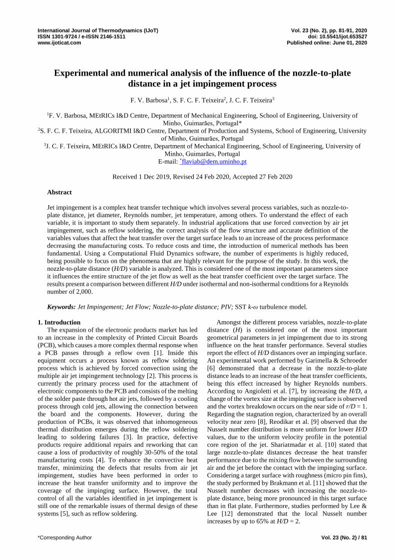
The numerical model, presented in Figure 1, consists of

a single jet impinging a cooper flat plate surface. The air

flows through a circular nozzle at a specific velocity, which

depends on the Reynolds number required in the study, and

at a constant temperature of about 120ºC. Since the Mach

number is below 0.3, the air jet flow is considered

incompressible. After the impingement, the air flow escapes

through the side walls. Considering this geometry and the

flow parameters, the Reynolds number obtained in this study

case is about 2,000. According to Viskanta [13], this flow

lies in the transition region, since at Re < 1,000 the flow field

exhibits a laminar flow behavior and at Re > 3,000 it presents

a fully turbulent behavior. This low Reynolds number value

represents a challenge in numerical simulations that applies

turbulence models to predict impinging jets.

In that sense, uniform velocity distribution was applied at

inlet while no-slip condition was implemented at both nozzle

and target plate. A constant temperature of 25ºC was

specified to the target surface and insulated wall was defined

at the nozzle plate. Pressure outlet boundary condition with

zero initial gauge pressure was applied to the open sides of

the domain.

Figure 1. Physical domain of the numerical model.

2.2 Governing Equations

The jet impingement system will be studied in two

dimensions. In that sense, the equations that define this

problem are the following:

𝜕𝑢

𝜕𝑥+𝜕𝑣

𝜕𝑦= 0 (1)

𝜕𝑢

𝜕𝑡+ 𝑢

𝜕𝑢

𝜕𝑥+ 𝑣

𝜕𝑢

𝜕𝑦= −

𝜕𝑝

𝜕𝑥+ 𝜇

𝜕2𝑢

𝜕𝑥2+ 𝜇

𝜕2𝑢

𝜕𝑦2 (2)

𝜕𝑣

𝜕𝑡+ 𝑢

𝜕𝑣

𝜕𝑥+ 𝑣

𝜕𝑣

𝜕𝑦= −

𝜕𝑝

𝜕𝑦+ 𝜇

𝜕2𝑣

𝜕𝑥2+ 𝜇

𝜕2𝑣

𝜕𝑦 (3)

𝜕𝑇

𝜕𝑡+ 𝑢

𝜕𝑇

𝜕𝑥+ 𝑣

𝜕𝑇

𝜕𝑦= 𝛼

𝜕2𝑇

𝜕𝑥2+ 𝛼

𝜕2𝑇

𝜕𝑦2 (4)

These governing equations are already simplified for an

incompressible flow. “Eq. (1)” represents the continuity

equation, “Eq. (2)” and “Eq. (3)” are the Navier-Stokes

equations in 2D, x-momentum and y-momentum respectively,

while “Eq. (4)” is the energy equation. The effect of gravity,

angular velocity vector and source term are neglected, since the

process in study is mainly influenced by convection.

Considering the equations presented above, it is possible to

identify the unknown and known variables. The unknowns are

the velocity in x-direction, u, the velocity in y-direction, v, the

pressure, p, and the temperature, T. The known variables are the

dynamic viscosity and thermal diffusivity of the fluid, µ and α

respectively.

2.3 Mathematical model and numerical method

According to several authors, it appears that the Shear Stress

Transport (SST) k-ω turbulence model proved to be both

accurate and computing time saving in engineering applications.

Zu et al. [14] compared different turbulence models with

experimental data and mentioned that the SST k-ω model

presents a better compromise between computational costs and

accuracy. Later, Ortega & Ortiz [15] verified a good agreement

between numerical and experimental data using this turbulence

model, being registered a maximum deviation of 8%. In

addition, Wen et al. [16] confirmed the good accuracy of the SST

k-ω model especially in the stagnation zones of the jets. A recent

study performed by Penumadu & Rao [17] revealed that the heat

transfer characteristics are well predicted by SST k-ω model,

mainly due to its ability to handle accurately regions with high

pressure gradients.

Due to the advantages pointed out by several studies

mentioned above, the SST k-ω model was selected for the

numerical simulation of the jet impingement. This model,

developed by Menter [18], applies the k-ω model in the near wall

region and switches to the k-ε model in the far field, combining

the advantages of both models. k-ω model performs much better

Int. J. of Thermodynamics (IJoT) Vol. 23 (No. 2) / 83

than k-ε model for boundary layer flows, however, it is

excessively sensitive to the freestream value of ω which

is not the case of the k-ε model. The combination between

the SST and the k-ω models improves the near wall

treatment since it gradually switches from a classical

low-Reynolds formulation on fine meshes to a log-wall

function formulation on coarser grids [19]. To describe

the flow near a wall, the SST k-ω model uses a low-

Reynolds number approach allowing the consideration of

the details in the viscous sublayer [20]. The equations of

the turbulence kinetic energy, k, and the specific

dissipation rate, ω, are presented in “Eq. (5)” and “Eq.

(6)”, respectively:

i k k k k

i j j

kk ku G Y S

t x x x

(5)

i

i j j

u G Y St x x x

(6)

where Г represents the effective diffusivity, G the

generation and Y the dissipation of the corresponding

variables. Dω is the cross-diffusion term while Sk and Sω

are the user-defined source terms [16].

To solve the pressure-velocity coupling, the SIMPLE

algorithm was applied. This algorithm uses a relationship

between velocity and pressure corrections to enforce

mass conservation and to obtain the pressure field [21].

Regarding the spatial discretization of momentum, a

second-order upwind was imposed while for the

dissipation rate and turbulent kinetic energy, a first order

upwind was applied. The computational models were

solved using a transient formulation based on a first-order

implicit method and the convergence criterion of 1E-3 for

continuity, momentum and turbulence equations and 1E-

6 for energy equation.

2.4 Mesh sensitivity

The mesh sensitivity analysis is extremely important

to determine the accuracy of the predictions as a function

of the mesh quality. To perform this analysis two

parameters were considered, the number of elements and

the bias factor. The bias factor is the ratio of the largest

to the smallest element, i.e. a higher bias factor implies a

greater refinement close to the walls. In that sense, a bias

factor of 4 and 8 was implemented in order to refine the

mesh near the target surface. However, a compromise

between the mesh refinement close to the walls and the

quality of the mesh must be ensured. Skewness, aspect

ratio and element quality factors were used as criteria for

element’s evaluation: Skewness determines how close to

the ideal a face or cell is (i.e. equilateral or equiangular),

a value close to zero defines equilaterality of the element;

aspect ratio is the ratio of the longest edge length to the

shortest edge length, being one for an equilateral cell;

element quality represents the ratio of the volume to the

sum of the square of the edge lengths for 2D elements or

square roots of the cub of the sum of the square of the

edge lengths for 3D elements, in which a value of 1

defines a perfect cube or square [22]. Nevertheless,

ensuring the recommended values is difficult since a

refinement implies smaller elements close to the walls

and higher elements in the remaining domain.

To analyze the meshes, the quality parameters of each

one, the computation time, as well as the y+ value, i.e. the

dimensionless distance of the first node to the wall [16], are

presented in Table 1. Looking at the computation time, it is

observed that the higher the number of elements, the greater

the simulation time as expected. In addition, it appears that

increasing the bias factor do not increases the complexity of

the mesh. In contrary, it seems to improve the convergence

of the results, thus the simulation time is 6 h higher for a

mesh with a lower bias factor. Regarding the mean wall y+,

it seems that its value is given by a combination between the

number of elements and the refinement close to the wall.

To determine the optimum grid size, the Nusselt number

variation over the target surface was analyzed and compared.

Since a larger Nusselt number represents a more effective

convection [23], this property allows to analyze the heat

transfer performance of the jet impingement. This property

represents the ratio between convection and conduction

across a fluid (Eq. 7).

Nu =ℎ ∙ 𝐷

𝑘𝑎𝑖𝑟 (7)

where h is the heat transfer coefficient, D the jet diameter

and kair the thermal conductivity of the air. The heat transfer

coefficient is obtained by “Eq. (8)” which represents the ratio

between the convective heat flux (�̇�) and the temperature

difference between the target surface (𝑇𝑤𝑎𝑙𝑙) and the air jet at

the inlet (𝑇𝑗𝑒𝑡) [26–28].

ℎ =�̇�

𝑇𝑤𝑎𝑙𝑙 − 𝑇𝑗𝑒𝑡 (8)

Table 1. Mesh Properties.

Mesh

1

(coars

e)

2

(mediu

m)

3

(fine)

4

(fine)

5

(fine)

Nº of

Element

s

10,0

80 36,800

124,50

0

124,50

0

336,00

0

Bias

factor 8 8 8 4 4

Skewnes

s 1.30×10-10

Aspect

Ratio 1.93 1.93 1.93 1.56 1.88

Element

Quality 0.82 0.82 0.82 0.90 0.83

Mean

wall y+ 5.16 2.66 1.31 2.2 1.03

Simulation Time

(t = 1s)

30

min 5h 11h 17h 3 days

As it can be observed in Figure 2, the Nusselt number

profile over the target surface is different in the five cases.

These results prove that the SST k-ω turbulence model is

sensitive to the quality of the mesh. Increasing the number of

elements, the stagnation point is clearly identified, in

contrast to the coarse and medium grids that are not able to

predict this point. Regarding the variation of the Nusselt

number over the plate, it is observed that a coarse grid

presents lower Nusselt number values close to the jet axis,

while the medium one has difficulties to predict the

stagnation point, showing higher Nusselt number values in

the vicinity of this point. Moreover, it is observed that the

mesh with 124,500 (bias = 8) presents similar values

compared with a mesh with 336,000 elements and a bias

factor of 4. The results demonstrate that, to ensure a good


accuracy of the simulation with less elements, a bias factor

must be applied. These observations are extremely important

since the higher the number of elements, the greater the

computation time and the memory required. In addition, the

data demonstrate that the improvement of the results using a

mesh with more elements does not justify the simulation time

required. Focusing on the Nusselt number obtained by the fine

grid at the stagnation point, it is observed that the maximum

value lies between the range 20 < Nu < 30. These values are in

accordance with numerical and experimental works found in

literature that apply a Re = 2,000 or close to this value

[27][28]. Considering the analysis presented above, it is

suggested that Mesh 3 presents the best conditions to conduct

the numerical simulations.

Figure 2. Nusselt number over the surface for different

meshes.

3. Experimental Apparatus

To perform a jet flow analysis, an experimental research

will be performed on a purpose-built test facility which has

been commissioned, using a Particle Image Velocimetry

(PIV) system. This method, depicted in Figure 3, allows the

measurement of the velocity field of the jets using a double-

pulse Nd:YAG laser and a CCD camera. The laser generates

a two-dimensional laser sheet which illuminates the

measurement region from the exit of the nozzles to the target

plate. The flow seeding is ensured by olive oil tracer particles

with a diameter between 1–3 μm introduced inside the

system using a smoke generator. This diameter complies

with the requirement of an accurate air flow tracking

presented by Melling [29]. The seeding particles follow the

instantaneous motion of the air and scatter the light that will

be captured by the CCD camera with a pixel resolution of

2560 × 2160 (5.5 Megapixel). The CCD camera captures

two consecutive images spaced by a short time interval in

order to visualize the displacement of the seeding particles

from one image to the next. This time between pulses was

defined through an analysis of the velocity field accuracy

using different times values. The data acquisition and

processing of the images are performed by the software

Dynamic Studio which divides the images into interrogation

areas and applies mathematical correlation to obtain velocity

vectors [30].

The experimental apparatus, whose scheme is presented

in Figure 4, consists of a ventilator (1) connected to a diffuser

(2) that directs the air to a stabilization chamber (3) in order

to reduce the turbulence. A flow regulator allows the control

of the air velocity that will flows through the orifice nozzle

(5). An acrylic pipe is attached to the stabilization chamber,

inside which a honeycomb structure (4) was placed to ensure

the uniformization of the flow. The PIV laser and camera

were positioned perpendicularly at a distance that allows to

capture the flow from the exit of the nozzles to the target

surface. The probe of the smoke generator is introduced

inside the stabilization chamber to ensure a correct

uniformization of the seeded flow throughout the pipe.

Figure 3. Schematic representation of a PIV system.

The target plate was placed above the nozzle plate on a

table that allows to control the spacing between the plate and

the nozzle. These experiments were conducted under

isothermal conditions (ambient temperature of about 20ºC)

and the nozzle-to-plate was varied from 2D to 7D. To ensure

a correct analysis of the PIV results 300 images were

analyzed for each case and the time-averaged velocity profile

was obtained. Since velocities around 7 m/s are expected, a

time between pulses around 100 µs was defined as a fixed

parameter of the laser. However, it was verified that

decreasing the nozzle-to-plate distance, higher turbulence

occurs between the target and nozzle plate, to minimize

measurements noise, the time between pulses was decreased

from 100 µs to 80 µs for 2 ≤ H/D ≤ 4.

The results obtained will be compared with the numerical

results performed with ANSYS FLUENT software. With

this analysis it is expected to validate the numerical results

and to prove that the SST k-ω model is suitable for the

prediction of a single jet impingement in a transition regime.

After this validation, the comparison between the flow

profile of an isothermal and non-isothermal jet will be

performed taking into consideration the influence of the

nozzle-to-plate distance. A Reynolds number of 2,000 at the

exit of the nozzle was ensured throughout the experiments.

The control of the air flow rate was performed using the fan

flow regulator.

Figure 4. Experimental Apparatus.


The resultant random error related to the PIV

measurements was obtained through a statistical analysis of

the data for 300 images, each case. This value was obtained

from the square root of the squared random error of velocity

components in x and y directions. Considering that these

error components are independent and follow a normal

distribution, for a confidence level of 95% [31], the

maximum random error obtained for the maximum velocity

recorded over the target surface was approximately 8%. The

uncertainty of the measurement is expected to decrease with

the increase of the sample size. According to [32], 2000

samples seems to be a good number to reduce the uncertainty

of the time-averaged velocities, u and v.

4. Results and Discussion

4.1 Flow Characterization

The flow characterization of an isothermal jet is

described in this section. The results obtained experimentally

and numerically were analyzed and compared for different

H/D.

Figure 5 shows the variation of the velocity profile of an

isothermal jet at different nozzle-to-plate distances. The

experimental results (right-hand side of each velocity

profile) are compared with those obtained numerically (left-

hand side). Even if smooth differences can be observed,

generally, both approaches present a good agreement.

The different regions of an impinging jet, according to

Martin [33], are identified and presented with detail in Figure

6: the initial free jet, the decaying jet, the stagnation region

and the wall jet. The first region is generated at the nozzle

exit where the maximum velocity is measured and

characterized by the interaction between the jet and the

surrounding air, inducing entrainment of mass, momentum

and energy [13]. The potential core, defined by Livingood &

Hrycak [34] as the distance from the nozzle exit to the

position where the jet velocity decays 95% of its maximum

velocity, is also clearly identified both numerically and

experimentally. From Figure 5, it seems that increasing H/D

leads to a decrease of the potential core length due to the

higher dissipation of the jet velocity, showing that low H/D

generated uniform velocity profile in this region. The end of

the core region is followed by the beginning of the decaying

region which is characterized by the linear variation of the

axial velocity and the jet width with the axial position [35].

As the flow gets closer to the wall, it loses axial velocity and

turns, generating a stagnation region in which the overall

velocity is near zero [8]. This point was clearly identified

experimentally at H/D equal to 2, 6 and 7, however, in the

other cases, the larger velocity vectors seems to cover-up this

point. Numerical data show a region close to the jet axis were

the velocity is near zero. The last region, the wall jet, is

identified once the air jet impacts on the target surface. After

the contact with the plate, the flow is divided into two

streams moving in opposite radial directions along the

surface, being observed a change of the flow direction from

axial (vertical axis y) to radial (longitudinal axis x) direction

[36]. The wall jet region is characterized by a maximum

radial velocity which moves away from the plate, since the

flow in this region is mainly radial with a growing boundary

layer [8]. Increasing the distance from the jet axis, the wall

jet entrains flow and increases in thickness, while the flow

velocity decreases. In the vicinity of the stagnation point, an

increase of the velocity is detected in all cases which can be

explained by a rapid acceleration of the flow due to larger

pressure gradients. Large heat transfer coefficients can be

obtained in this specific region, in the transition from the

laminar to turbulent boundary layer [37]. The separation of

the flow occurs where the boundary layer leaves the surface

of the plate and seems to occur closer to the impinging point

at low nozzle-to-plate distances.

Figure 5. Jet flow velocity profile. The right-hand side presents

the experimental data while the left-hand side depicts the results

obtained numerically.

As Figure 5 shows, the wall jet thickness increases with

decreasing the nozzle to plate distance due to higher local

pressure induced by strong interactions between the jet and

the surrounding air. Furthermore, results demonstrated that

the wall jet region increases in the radial direction with the

increase of H/D, which is in accordance with other confined

jet impingement studies at higher Reynolds numbers [7]

[37]. Focusing on the vortices generated on both sides of the

jet axis, it seems that the higher the nozzle-to-plate distance,

the lower the magnitude of the vortices generated, which is

essentially due to the larger space for the flow to develop.


Figure 6. Flow regions of an impinging jet.

Through the previous analysis, it seems that both

numerical and experimental results predict with accuracy the

flow structure of a single jet in the transition region.

Focusing on quantitative data, the time-averaged velocity

over the target surface at different H/D values was plotted

and presented in Figure 7.

Figure 7. Time-averaged velocity over the target surface at

different H/D and Re = 2,000.

Considering an air jet at ambient temperature (≈ 20ºC)

impinging a flat plate at the same temperature, the results

obtained experimentally (Figure 7) shows the evolution of

the nondimensional velocity, U/Uj, where U is the time-

averaged velocity obtained by PIV measurements and Uj the

maximum velocity recorded at the nozzle exit, over the target

surface. The maximum velocity is achieved for a nozzle-to-

plate value of 2, at a distance from the jet axis of

approximately x/D = 2. This is in accordance with the jet

flow structure presented in Figure 5, small confined spaces

induce a stronger interaction between the surrounding air and

the vortices generated by the jet impingement, leading to

higher velocities over the wall. Results also show that the

higher the nozzle-to-plate distance, the lower the velocity in

the vicinity of the stagnation point. The maximum value is

recorded in all cases at a distance from the jet axis (x/D)

between 2 and 4, increasing with the increase of H/D.

Moreover, as it was expected, the jet wall increases with

increasing H/D, leading to a smoother decrease of the

velocity throughout the target plate. For H/D = 2, an

interesting phenomenon is observed. After reaching the

maximum velocity, its value starts to decrease, achieving a

minimum velocity at approximately x/D = 4. From this point,

as opposed to the other cases, the velocity rose again

achieving a second maximum point at about x/D = 6. This

secondary point was identified in several studies, mentioned

in Zuckerman & Lior [35] and Viskanta [13], being

attributed to the transition of the boundary layer from

laminar to turbulent flow along the wall. A secondary

velocity peak was also identified in H/D = 3 at approximately

x/D = 8. However, with the increase of the nozzle-to-plate

distance, the interactions between the jet and the surrounding

air in the confined space decreases, and since the Reynolds

number is low, no secondary peak was identified at higher

H/D values. Viskanta [13] summarized the influence of the

nozzle-to-plate distances smaller than the jet potential core

length on the radial distribution of convective heat transfer

coefficient and pointed out three main factors: (a) the laminar

boundary layer behavior under strongly accelerated

surrounding flow in the vicinity of the stagnation point; (b)

the interaction of large-scale turbulence induced in the

mixing zone; but also (c) the transition of the boundary layer

from laminar to turbulent over the wall jet.

Regarding the stagnation point, it is detected with a

higher accuracy at H/D = 2, with a velocity value very close

to zero at the jet axis, as it is expected. However, this is not

observed in the other cases. This can be explained by the fact

that, to detect this point with accuracy, an interrogation area

with a higher resolution than the one used in this experiment

(32 × 32 pixels) must be used. To reduce the lag between the

expected value (U = 0) and the ones obtained experimentally,

the focus angle of the camera should be reduced to the zone

that we intend to analyze, in this case the stagnation region.

However, since in this experiment it is expected to

characterize all the flow, from the nozzle exit to the target

plate, the focus angle must be large. Another reason to

explain this lag is related to factors that can generate

systematic errors such as the concentration of particles as

well as the time between pulses. These are two fundamental

factors that can decrease the accuracy of the PIV

measurements. It was verified that even if the same Reynolds

number was maintained throughout the experiments, since

higher velocities were recorded over the wall region for

lower nozzle-to-plate distance, we had to decrease the time

between pulses to increase the accuracy of the results.

Meaning that, for 2 ≤ H/D ≤ 5 a lower time between pulses

was implemented compared with H/D of 6 and 7. This

adjustment of the time between pulse in function of the flow

velocity is crucial to ensure accurate results.

4.2 Numerical model validation

The experimental data was used for the validation of the

numerical model. In that sense the time-averaged velocity

over the target surface at different nozzle-to-plate spacings

for a Reynolds number of 2,000 obtained numerically were

compared with the experimental results. Observing in detail

Figure 5 which shows the velocity field of a single jet flow

(Re = 2,000) at a different nozzle-to-plate distance, it is clear

that the SST k-ω model do not predict with accuracy the

potential core in the case of H/D equal to 6 and 7. While the

experimental data demonstrated clearly a decrease of the

potential core length with the increase of the nozzle-to-plate

distance, this decrease is smoother in the case of the

numerical data. As mentioned previously, the increase of

H/D leads to a decrease of the potential core length due to

the higher dissipation of the jet velocity. However, this

dissipation of velocity for higher H/D values is not

accurately predicted numerically. This shows that the

numerical model must be improved to increase the accuracy

of the prediction in the stagnation region. Furthermore,

regarding the wall jet region, the decrease of the wall

thickness with increasing H/D values is easily observed

through the numerical results.

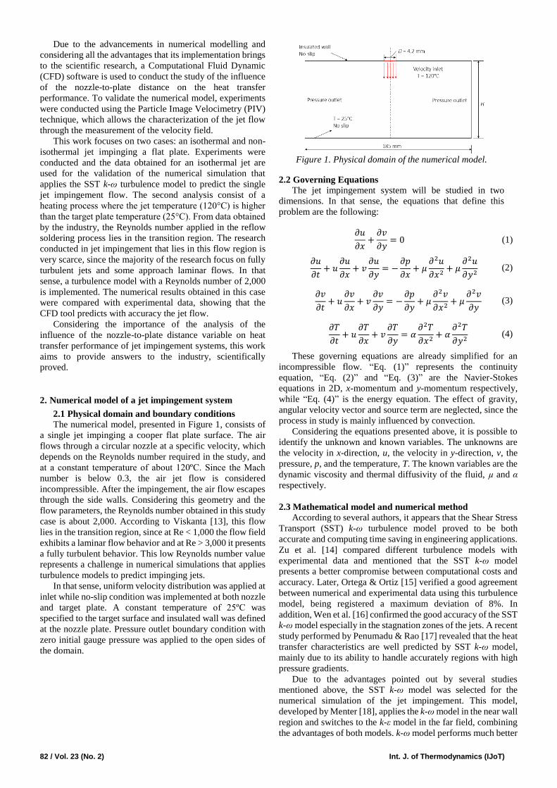
From the flow velocity over the target surface, the results

obtained numerically were plotted and presented in Figure 8.

The secondary velocity peak was identified in the case of

H/D = 2 between 6 ≤ x/D ≤ 8, even if this value is lower than

the one obtained experimentally U/Uj = 0.2 against U/Uj =

0.34. Regarding the stagnation point, it was not predicted

with accuracy in any case, a value of U/Uj = 0.1 was obtained

0

0.1

0.2

0.3

0.4

0.5

0.6

0.7

0 2 4 6 8 10

U/U

j

x/D

H/D = 2

H/D = 3

H/D = 4

H/D = 5

H/D = 6

H/D = 7


instead of 0. However, this point was also difficult to identify

experimentally.

Looking at the maximum velocity value, it was recorded

in the vicinity of the stagnation point, as it was expected,

however, in contrast to the experimental data, this peak was

detected at x/D = 1.2 for all the nozzle to plate distances.

Regarding the maximum velocity, its value seems to

decrease with increasing H/D, as expected, however this

decrease is more pronounced in the experimental results. For

H/D = 2, the nondimensional velocity U/Uj obtained both

experimentally and numerically is close to 0.7, while in the

other cases, it is predicted to be around 0.6 by the turbulence

model. In contrast, the experimental results show a decrease

from 0.7 at H/D = 2 to approximately 0.3 at H/D = 7. This

discrepancy between numerical and experimental results

show that the effects of the surrounding air on the jet flow

development are more pronounced experimentally. Even if

the measurement zone is enclosed by an acrylic box, it is

difficult to ensure constant temperature and humidity

conditions throughout the experiments.

Figure 8. SST k-ω velocity over the target surface at different H/D

and Re = 2,000.

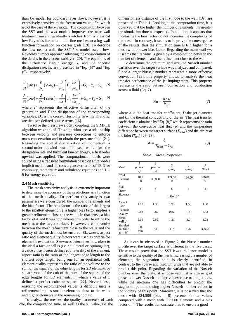
The variation of U/Uj throughout the jet axis in the case

of H/D equal to 2 and 7 was presented in Figure 9. The

profile predicted numerically is very close to that obtained

experimentally, with a maximum and constant velocity

recorded close to the jet axis (maximum y value). After

leaving the nozzle, the air jet started to entrain surrounding

air, decreasing the velocity which became steeper near the

target plate. This velocity decrease was more pronounced at

H/D = 7, due to the lower potential core length compared

with H/D = 2. The minimum velocity value was achieved at

the stagnation point, as expected. However, it is clear that the

velocity profile obtained numerically is more uniform

compared with the experimental ones. This deviation is

essentially due to external factors, discussed in section 4.1,

which are not considered by the numerical simulation.

Moreover, it is verified that higher velocities are recorded

over the jet axis at lower nozzle-to-plate spacing, which is in

agreement with the previous results. A lower H/D leads to an

increase of turbulence between the main jet and the wall jet.

Figure 9. Variation of the mean velocity through the jet axis.

The comparison between numerical end experimental

results show a good agreement between the two approaches,

essentially regarding qualitative data. The SST k-ω model

was able to predict with accuracy the jet flow structure;

however, it fails in the prediction of the potential core. The

maximum velocity was predicted in the vicinity of the

stagnation point and decreases with increasing H/D.

Focusing on the quantitative data, the maximum velocity was

accurately predicted in the case of H/D = 2 while for higher

H/D values it was over predicted. The secondary peak was

also identified numerically even if the value was under

predicted compared with the experimental data. In general,

we can conclude that the SST k-ω model presents good

qualitative predictions of the single jet impingement flow at

Reynolds number in the transition region. If quantitative

results are important for the analysis, this turbulence model

is more accurate for higher Reynolds numbers.

4.3 Non-isothermal jet

After the validation of the numerical model of a single jet

impingement using the SST k-ω model, a non-isothermal jet,

with the same geometrical variables implemented in the

isothermal jet, was analyzed numerically.

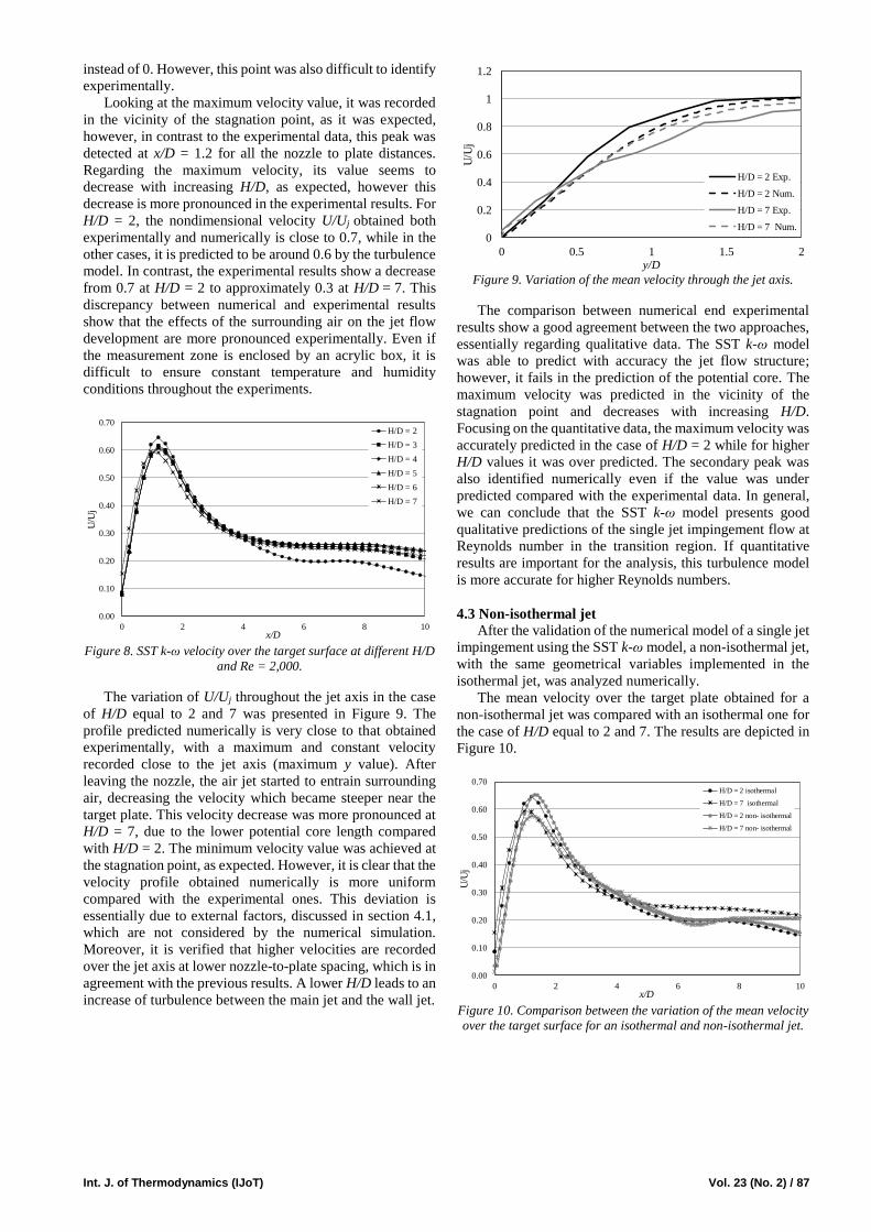
The mean velocity over the target plate obtained for a

non-isothermal jet was compared with an isothermal one for

the case of H/D equal to 2 and 7. The results are depicted in

Figure 10.

Figure 10. Comparison between the variation of the mean velocity

over the target surface for an isothermal and non-isothermal jet.

0.00

0.10

0.20

0.30

0.40

0.50

0.60

0.70

0 2 4 6 8 10

U/U

j

x/D

H/D = 2

H/D = 3

H/D = 4

H/D = 5

H/D = 6

H/D = 7

0

0.2

0.4

0.6

0.8

1

1.2

0 0.5 1 1.5 2

U/U

j

y/D

H/D = 2 Exp.

H/D = 2 Num.

H/D = 7 Exp.

H/D = 7 Num.

0.00

0.10

0.20

0.30

0.40

0.50

0.60

0.70

0 2 4 6 8 10

U/U

j

x/D

H/D = 2 isothermal

H/D = 7 isothermal

H/D = 2 non- isothermal

H/D = 7 non- isothermal


Comparing the velocity profiles for the case of an

isothermal and non-isothermal jet, it is interesting to observe

that the peak velocity is reached at the vicinity of the

stagnation point, as expected, but at a higher distance from

this point compared with the isothermal jet, x/D ≈ 1.4,

against x/D ≈ 1.2. These results show that increasing the

temperature difference between the jet and the target plate,

the development of the boundary layer throughout the target

plate is slightly different compared with isothermal jets. It

seems that the acceleration of the radial flow in the vicinity

of the stagnation point is higher in the isothermal case.

However, no relevant difference is observed in non-

dimensional velocity U/Uj value, being approximately 0.65

at H/D = 2 and close to 0.6 for H/D = 7. Focusing on the

secondary peak, it was predicted at a nozzle-to-plate distance

of 7 for the case of a non-isothermal jet, showing that the jet

temperature and velocity leads to a higher mixing between

the jet and the surrounding air.

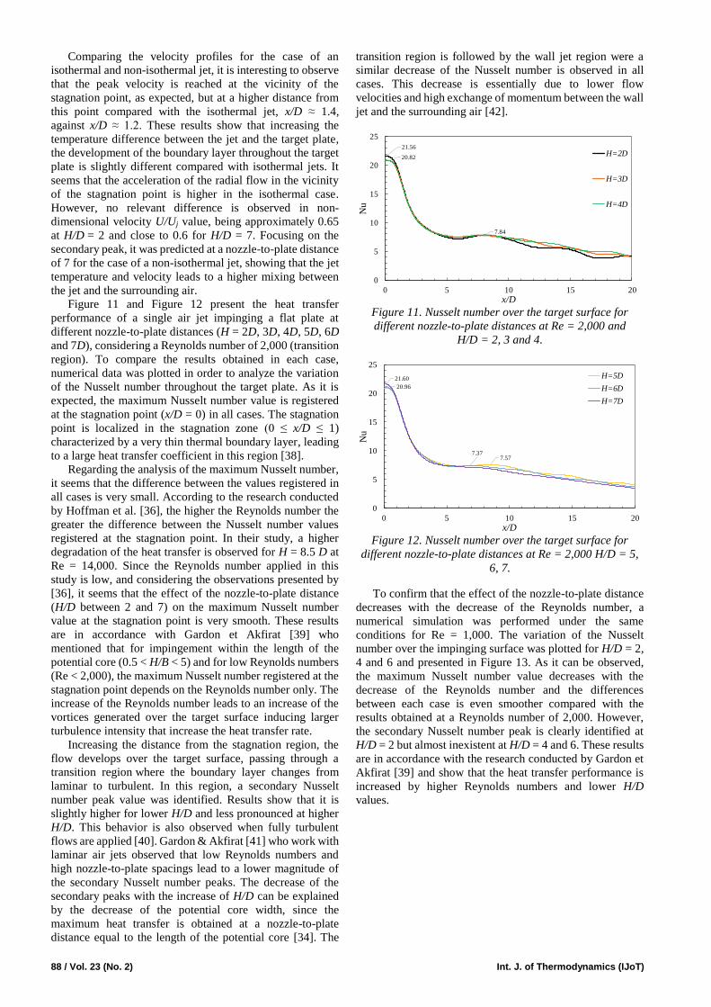
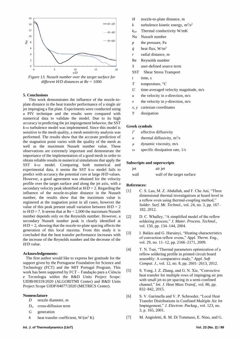
Figure 11 and Figure 12 present the heat transfer

performance of a single air jet impinging a flat plate at

different nozzle-to-plate distances (H = 2D, 3D, 4D, 5D, 6D

and 7D), considering a Reynolds number of 2,000 (transition

region). To compare the results obtained in each case,

numerical data was plotted in order to analyze the variation

of the Nusselt number throughout the target plate. As it is

expected, the maximum Nusselt number value is registered

at the stagnation point (x/D = 0) in all cases. The stagnation

point is localized in the stagnation zone (0 ≤ x/D ≤ 1)

characterized by a very thin thermal boundary layer, leading

to a large heat transfer coefficient in this region [38].

Regarding the analysis of the maximum Nusselt number,

it seems that the difference between the values registered in

all cases is very small. According to the research conducted

by Hoffman et al. [36], the higher the Reynolds number the

greater the difference between the Nusselt number values

registered at the stagnation point. In their study, a higher

degradation of the heat transfer is observed for H = 8.5 D at

Re = 14,000. Since the Reynolds number applied in this

study is low, and considering the observations presented by

[36], it seems that the effect of the nozzle-to-plate distance

(H/D between 2 and 7) on the maximum Nusselt number

value at the stagnation point is very smooth. These results

are in accordance with Gardon et Akfirat [39] who

mentioned that for impingement within the length of the

potential core (0.5 < H/B < 5) and for low Reynolds numbers

(Re < 2,000), the maximum Nusselt number registered at the

stagnation point depends on the Reynolds number only. The

increase of the Reynolds number leads to an increase of the

vortices generated over the target surface inducing larger

turbulence intensity that increase the heat transfer rate.

Increasing the distance from the stagnation region, the

flow develops over the target surface, passing through a

transition region where the boundary layer changes from

laminar to turbulent. In this region, a secondary Nusselt

number peak value was identified. Results show that it is

slightly higher for lower H/D and less pronounced at higher

H/D. This behavior is also observed when fully turbulent

flows are applied [40]. Gardon & Akfirat [41] who work with

laminar air jets observed that low Reynolds numbers and

high nozzle-to-plate spacings lead to a lower magnitude of

the secondary Nusselt number peaks. The decrease of the

secondary peaks with the increase of H/D can be explained

by the decrease of the potential core width, since the

maximum heat transfer is obtained at a nozzle-to-plate

distance equal to the length of the potential core [34]. The

transition region is followed by the wall jet region were a

similar decrease of the Nusselt number is observed in all

cases. This decrease is essentially due to lower flow

velocities and high exchange of momentum between the wall

jet and the surrounding air [42].

Figure 11. Nusselt number over the target surface for

different nozzle-to-plate distances at Re = 2,000 and

H/D = 2, 3 and 4.


different nozzle-to-plate distances at Re = 2,000 H/D = 5,

6, 7.

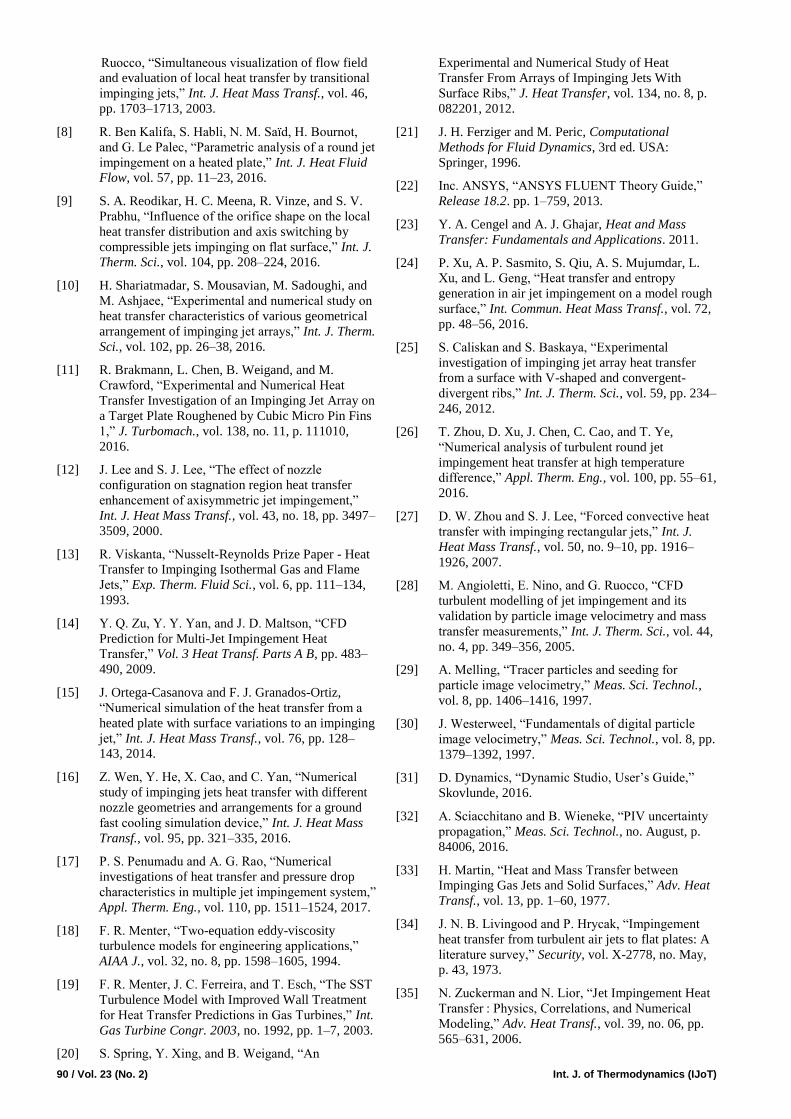
To confirm that the effect of the nozzle-to-plate distance

decreases with the decrease of the Reynolds number, a

numerical simulation was performed under the same

conditions for Re = 1,000. The variation of the Nusselt

number over the impinging surface was plotted for H/D = 2,

4 and 6 and presented in Figure 13. As it can be observed,

the maximum Nusselt number value decreases with the

decrease of the Reynolds number and the differences

between each case is even smoother compared with the

results obtained at a Reynolds number of 2,000. However,

the secondary Nusselt number peak is clearly identified at

H/D = 2 but almost inexistent at H/D = 4 and 6. These results

are in accordance with the research conducted by Gardon et

Akfirat [39] and show that the heat transfer performance is

increased by higher Reynolds numbers and lower H/D

values.

21.56

20.82

7.84

0

5

10

15

20

25

0 5 10 15 20

Nu

x/D

H=2D

H=3D

H=4D

20.96

7.577.37

21.60

0

5

10

15

20

25

0 5 10 15 20

Nu

x/D

H=5D

H=6D

H=7D



different H/D distances at Re = 1000.

5. Conclusions

This work demonstrates the influence of the nozzle-to-

plate distance in the heat transfer performance of a single air

jet impinging a flat plate. Experiments were conducted using

a PIV technique and the results were compared with

numerical data to validate the model. Due to its high

accuracy in predicting the jet impingement behavior, the SST

k-ω turbulence model was implemented. Since this model is

sensitive to the mesh quality, a mesh sensitivity analysis was

performed. The results show that the accurate prediction of

the stagnation point varies with the quality of the mesh as

well as the maximum Nusselt number value. These

observations are extremely important and demonstrate the

importance of the implementation of a good mesh in order to

obtain reliable results in numerical simulations that apply the

SST k-ω model. Comparing both numerical and

experimental data, it seems the SST k-ω model fails to

predict with accuracy the potential core at large H/D values.

However, a good agreement was obtained for the velocity

profile over the target surface and along the jet axis, with a

secondary velocity peak identified at H/D = 2. Regarding the

influence of the nozzle-to-plate distance in the Nusselt

number, the results show that the maximum value is

registered at the stagnation point in all cases, however the

value of this peak present small variation between H/D = 2

to H/D = 7. It seems that at Re < 2,000 the maximum Nusselt

number depends only on the Reynolds number. However, a

secondary Nusselt number peak is clearly identified at

H/D = 2, showing that the nozzle-to-plate spacing affects the

generation of this local maxima. From this study it is

concluded that the heat transfer performance increases with

the increase of the Reynolds number and the decrease of the

H/D value.

Acknowledgements:

The first author would like to express her gratitude for the

support given by the Portuguese Foundation for Science and

Technology (FCT) and the MIT Portugal Program. This

work has been supported by FCT – Fundação para a Ciência

e Tecnologia within the R&D Units Project Scope:

UIDB/00319/2020 (ALGORITMI Center) and R&D Units

Project Scope UIDP/04077/2020 (METRICS Center).

Nomenclature

D nozzle diameter, m

Dω cross-diffusion term

G generation

h heat transfer coefficient, W/(m2 K)

H nozzle-to-plate distance, m

k turbulence kinetic energy, m2/s2

kair Thermal conductivity W/mK

Nu Nusselt number

p the pressure, Pa

�̇� heat flux, W/m2

r radial distance, m

Re Reynolds number

S user-defined source term

SST Shear Stress Transport

t time, s

T temperature, °C

U time-averaged velocity magnitude, m/s

u the velocity in x-direction, m/s

v the velocity in y-direction, m/s

x, y cartesian coordinates

Y dissipation

Greek symbols

Г effective diffusivity

α thermal diffusivity, m2/s

µ dynamic viscosity, m/s

ω specific dissipation rate, 1/s

Subscripts and superscripts

jet air jet

wall wall of the target surface

References:

[1] C. S. Lau, M. Z. Abdullah, and F. Che Ani, “Three

dimensional thermal investigations at board level in

a reflow oven using thermal‐coupling method,”

Solder. Surf. Mt. Technol., vol. 24, no. 3, pp. 167–

182, 2012.

[2] D. C. Whalley, “A simplified model of the reflow

soldering process,” J. Mater. Process. Technol.,

vol. 150, pp. 134–144, 2004.

[3] I. Balázs and G. Harsányi, “Heating characteristics

of convection reflow ovens,” Appl. Therm. Eng.,

vol. 29, no. 11–12, pp. 2166–2171, 2009.

[4] T. N. Tsai, “Thermal parameters optimization of a

reflow soldering profile in printed circuit board

assembly: A comparative study,” Appl. Soft

Comput. J., vol. 12, no. 8, pp. 2601–2613, 2012.

[5] S. Yong, J. Z. Zhang, and G. N. Xie, “Convective

heat transfer for multiple rows of impinging air jets

with small jet-to-jet spacing in a semi-confined

channel,” Int. J. Heat Mass Transf., vol. 86, pp.

832–842, 2015.

[6] S. V. Garimella and V. P. Schroeder, “Local Heat

Transfer Distributions in Confined Multiple Air Jet

Impingement,” J. Electron. Packag., vol. 123, no.

3, p. 165, 2001.

[7] M. Angioletti, R. M. Di Tommaso, E. Nino, and G.

0

2

4

6

8

10

12

14

16

0 5 10 15 20

Nu

x/D

H=2D

H=4D

H=6D


Ruocco, “Simultaneous visualization of flow field

and evaluation of local heat transfer by transitional

impinging jets,” Int. J. Heat Mass Transf., vol. 46,

pp. 1703–1713, 2003.

[8] R. Ben Kalifa, S. Habli, N. M. Saïd, H. Bournot,

and G. Le Palec, “Parametric analysis of a round jet

impingement on a heated plate,” Int. J. Heat Fluid

Flow, vol. 57, pp. 11–23, 2016.

[9] S. A. Reodikar, H. C. Meena, R. Vinze, and S. V.

Prabhu, “Influence of the orifice shape on the local

heat transfer distribution and axis switching by

compressible jets impinging on flat surface,” Int. J.

Therm. Sci., vol. 104, pp. 208–224, 2016.

[10] H. Shariatmadar, S. Mousavian, M. Sadoughi, and

M. Ashjaee, “Experimental and numerical study on

heat transfer characteristics of various geometrical

arrangement of impinging jet arrays,” Int. J. Therm.

Sci., vol. 102, pp. 26–38, 2016.

[11] R. Brakmann, L. Chen, B. Weigand, and M.

Crawford, “Experimental and Numerical Heat

Transfer Investigation of an Impinging Jet Array on

a Target Plate Roughened by Cubic Micro Pin Fins

1,” J. Turbomach., vol. 138, no. 11, p. 111010,

2016.

[12] J. Lee and S. J. Lee, “The effect of nozzle

configuration on stagnation region heat transfer

enhancement of axisymmetric jet impingement,”

Int. J. Heat Mass Transf., vol. 43, no. 18, pp. 3497–

3509, 2000.

[13] R. Viskanta, “Nusselt-Reynolds Prize Paper - Heat

Transfer to Impinging Isothermal Gas and Flame

Jets,” Exp. Therm. Fluid Sci., vol. 6, pp. 111–134,

1993.

[14] Y. Q. Zu, Y. Y. Yan, and J. D. Maltson, “CFD

Prediction for Multi-Jet Impingement Heat

Transfer,” Vol. 3 Heat Transf. Parts A B, pp. 483–

490, 2009.

[15] J. Ortega-Casanova and F. J. Granados-Ortiz,

“Numerical simulation of the heat transfer from a

heated plate with surface variations to an impinging

jet,” Int. J. Heat Mass Transf., vol. 76, pp. 128–

143, 2014.

[16] Z. Wen, Y. He, X. Cao, and C. Yan, “Numerical

study of impinging jets heat transfer with different

nozzle geometries and arrangements for a ground

fast cooling simulation device,” Int. J. Heat Mass

Transf., vol. 95, pp. 321–335, 2016.

[17] P. S. Penumadu and A. G. Rao, “Numerical

investigations of heat transfer and pressure drop

characteristics in multiple jet impingement system,”

Appl. Therm. Eng., vol. 110, pp. 1511–1524, 2017.

[18] F. R. Menter, “Two-equation eddy-viscosity

turbulence models for engineering applications,”

AIAA J., vol. 32, no. 8, pp. 1598–1605, 1994.

[19] F. R. Menter, J. C. Ferreira, and T. Esch, “The SST

Turbulence Model with Improved Wall Treatment

for Heat Transfer Predictions in Gas Turbines,” Int.

Gas Turbine Congr. 2003, no. 1992, pp. 1–7, 2003.

[20] S. Spring, Y. Xing, and B. Weigand, “An

Experimental and Numerical Study of Heat

Transfer From Arrays of Impinging Jets With

Surface Ribs,” J. Heat Transfer, vol. 134, no. 8, p.

082201, 2012.

[21] J. H. Ferziger and M. Peric, Computational

Methods for Fluid Dynamics, 3rd ed. USA:

Springer, 1996.

[22] Inc. ANSYS, “ANSYS FLUENT Theory Guide,”

Release 18.2. pp. 1–759, 2013.

[23] Y. A. Cengel and A. J. Ghajar, Heat and Mass

Transfer: Fundamentals and Applications. 2011.

[24] P. Xu, A. P. Sasmito, S. Qiu, A. S. Mujumdar, L.

Xu, and L. Geng, “Heat transfer and entropy

generation in air jet impingement on a model rough

surface,” Int. Commun. Heat Mass Transf., vol. 72,

pp. 48–56, 2016.

[25] S. Caliskan and S. Baskaya, “Experimental

investigation of impinging jet array heat transfer

from a surface with V-shaped and convergent-

divergent ribs,” Int. J. Therm. Sci., vol. 59, pp. 234–

246, 2012.

[26] T. Zhou, D. Xu, J. Chen, C. Cao, and T. Ye,

“Numerical analysis of turbulent round jet

impingement heat transfer at high temperature

difference,” Appl. Therm. Eng., vol. 100, pp. 55–61,

2016.

[27] D. W. Zhou and S. J. Lee, “Forced convective heat

transfer with impinging rectangular jets,” Int. J.

Heat Mass Transf., vol. 50, no. 9–10, pp. 1916–

1926, 2007.

[28] M. Angioletti, E. Nino, and G. Ruocco, “CFD

turbulent modelling of jet impingement and its

validation by particle image velocimetry and mass

transfer measurements,” Int. J. Therm. Sci., vol. 44,

no. 4, pp. 349–356, 2005.

[29] A. Melling, “Tracer particles and seeding for

particle image velocimetry,” Meas. Sci. Technol.,

vol. 8, pp. 1406–1416, 1997.

[30] J. Westerweel, “Fundamentals of digital particle

image velocimetry,” Meas. Sci. Technol., vol. 8, pp.

1379–1392, 1997.

[31] D. Dynamics, “Dynamic Studio, User’s Guide,”

Skovlunde, 2016.

[32] A. Sciacchitano and B. Wieneke, “PIV uncertainty

propagation,” Meas. Sci. Technol., no. August, p.

84006, 2016.

[33] H. Martin, “Heat and Mass Transfer between

Impinging Gas Jets and Solid Surfaces,” Adv. Heat

Transf., vol. 13, pp. 1–60, 1977.

[34] J. N. B. Livingood and P. Hrycak, “Impingement

heat transfer from turbulent air jets to flat plates: A

literature survey,” Security, vol. X-2778, no. May,

p. 43, 1973.

[35] N. Zuckerman and N. Lior, “Jet Impingement Heat

Transfer : Physics, Correlations, and Numerical

Modeling,” Adv. Heat Transf., vol. 39, no. 06, pp.

565–631, 2006.


[36] H. M. Hofmann, M. Kind, and H. Martin,

“Measurements on steady state heat transfer and

flow structure and new correlations for heat and

mass transfer in submerged impinging jets,” Int. J.

Heat Mass Transf., vol. 50, no. 19–20, pp. 3957–

3965, 2007.

[37] Y. O. Æ. E. Baydar, “Flow structure and heat

transfer characteristics of an unconfined impinging

air jet at high jet Reynolds numbers,” pp. 1315–

1322, 2008.

[38] L. Xin, L. A. Gabour, and J. H. Lienhard V,

“Stagnation-Point Heat Transfer During

Impingement of Laminar Liquid Jets : Analysis

Including,” J. Heat Transfer, vol. 115, no.

February, pp. 99–106, 1993.

[39] R. Gardon and C. Akfirat, “Heat Transfer

Characteristics of Impinging Two-Dimensional Air

Jets,” J. Heat Transf. Asme, pp. 1–7, 1966.

[40] V. Katti and S. V Prabhu, “Experimental study and

theoretical analysis of local heat transfer

distribution between smooth flat surface and

impinging air jet from a circular straight pipe

nozzle,” vol. 51, pp. 4480–4495, 2008.

[41] R. Gardon and C. Akfirat, “The role of turbulence

in determining the heat-transfer characteristics of

impinging jets,” Int. J. Heat Mass Transf., vol. 8,

pp. 1261–1272, 1965.

[42] V. Katti and S. V Prabhu, “Experimental study and

theoretical analysis of local heat transfer

distribution between smooth flat surface and

impinging air jet from a circular straight pipe

nozzle,” Int. J. Heat Mass Transf., vol. 51, pp.

4480–4495, 2008.

Experimental and numerical analysis of the influence of ...

Documents

Transcript of Experimental and numerical analysis of the influence of ...