Experiment Guide: RC Filters and LabVIEW Description and Background In this lab you will (a) manipulate instruments manually to determine the input-output characteristics of an RC filter, and then (b) use an instrument control system called LabVIEW (made by National Instruments, Inc.) to measure and plot RC filter characteristics automatically. A. RC Filter Characteristics Figure 1 below shows an RC filter connected to a sinusoidal voltage source. This circuit is termed a two-port circuit (see Fig. 2) where the voltage source produces the input voltage Vin and the output voltage Vout appears across resistor R.

Figure 1. RC filter with series capacitor and output resistor R (HPF).

+

-

VoutV

in

+

-

RC

Figure 2. Two-port circuit.

vin

vout

Recall that we customarily represent an AC voltage as a periodic function of time such as V(t) = V0cos(ωt) where V0 is the amplitude of the voltage, t is time, and ω is the so-called angular frequency, whose units are radians per second. The angular frequency is related to the “ordinary” frequency, f, measured in Hertz, by ω = 2πf. For example, if the frequency, f, of the ordinary power line voltage in the U. S. is 60 Hz, then the associated angular frequency, ω, is 377 radians/s (2π×60). Transfer Function A two-port circuit is characterized by its so-called transfer function, whose magnitude is defined as |Vout/Vin|, where Vout and Vin are phasor (has both amplitude and phase) voltages (as indicated by the boldface type). The variation of the transfer function with frequency characterizes the frequency response of the circuit (a high-pass filter, low-pass filter or band-pass filter).

If you analyze the RC circuit of Fig. 1 using Kirchhoff’s voltage law, the phasor voltages Vout and Vin, the resistance R and the impedance of the capacitor ZC = 1/jωC, you can show that the magnitude of the transfer function is

2)ωRC(1ωRC+

=in

out

VV (1)

An approximate log-log plot of transfer function magnitude vs. angular frequency is shown in Figure 3:

in

out

VV

( )radωRCB1=ω

in

out

VV

( )radωRCB1=ω

1

2/1

in

out

VV

in

out

VV

( )radω ( )radωRCB1=ω

RCB1=ω

in

out

VV

in

out

VV

( )radω ( )radωRCB1=ω

RCB1=ω

1

2/1

Fig. 3. Log-log plot of transfer function magnitude vs. angular frequency for the HPF. The filter characteristic is shown in Figure 3 as a high-pass filter which passes frequencies higher than τω /1/1 == RCB , which is the critical frequency used to indicate the pass band. For this high-pass filter (HPF) the pass band is Bωω > . The critical frequency is defined as the frequency at which the output voltage amplitude drops to 2/1 of the input voltage amplitude (also called 3 dB point in decibel scales. Please refer to Chapter 6 for more information on Decibels and Bode plots). In order to plot the whole frequency response, one has to plot over a frequency range that covers Bω (e.g. BB ωωω 101.0 << ). If we reverse the positions of R and C in the filter circuit (Figure 4), we obtain the transfer function and filter characteristic shown below:

Fig. 4. Circuit with a series resistor R and the capacitor C as the output element (LPF).

+

-

VoutV

in

+

-

RC

2)ωRC(11

+=

in

out

VV (2)

in

out

VV

( )radωRCB1=ω

1

in

out

VV

( )radωRCB1=ω

12/1

in

out

VV

in

out

VV

( )radω ( )radωRCB1=ω

RCB1=ω

1

in

out

VV

in

out

VV

( )radω ( )radωRCB1=ω

RCB1=ω

12/1

Fig. 5. Log-log plot of transfer function magnitude vs. angular frequency for the LPF. The filter characteristic is shown in Figure 5 as a low pass filter which passes frequencies lower than τω /1/1 == RCB . For this low-pass filter (LPF) the pass band is Bωω <<0 .

Figure 6. below shows a series resonant circuit, with voltage read across the resistor. This acts as a bandpass filter.

The circuit’s resonant frequency, ω0, is the frequency where the impedance is entirely due to the resistance. At resonance, the reactance of the capacitor cancels out the reactance of the inductor so they must be equal in magnitude. The quality factor, Q, of a series RLC filter is defined as the ratio of the inductive reactance to the resistance, at the resonant frequency:

R

L C

Fig. 6. Series RLC Bandpass Filter, with AC source.

RLf

RLQ 00 2πω

==

Fig. 7. Plots of Transfer Function magnitude, for different values of Qs, the quality factor of a series RLC circuit. Note that this plot is not on a log-log scale (which Bode plots feature).

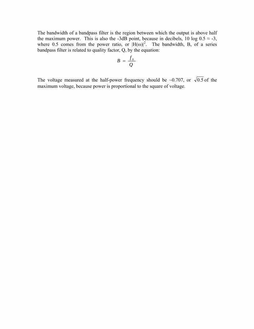
The bandwidth of a bandpass filter is the region between which the output is above half the maximum power. This is also the -3dB point, because in decibels, 10 log 0.5 ≈ -3, where 0.5 comes from the power ratio, or |H(ω)|2. The bandwidth, B, of a series bandpass filter is related to quality factor, Q, by the equation: The voltage measured at the half-power frequency should be ~0.707, or 5.0 of the maximum voltage, because power is proportional to the square of voltage.

QfB 0=

Procedures P1. Connect a 10kΩ resistor and a (non-polarized) 0.1 µF capacitor in series with a signal generator as shown in Fig 1, making sure that your oscilloscope ground and the signal generator ground are connected together. Set the signal generator to output a 0.5V-Vpp sine wave. Measure and plot the amplitude of the voltage across the resistor versus frequency on log-log graph paper. You can download log-log graph paper from the EE 40 web site. First figure out the frequency range and the step of the sample points you are going to use. Should you make the step constant over the range? (hint: take more points when the curve turns, take less points when it is constant.) P2. Reverse the order of the two components as shown in Fig 4 and repeat. Plot the amplitude vs. frequency in a log-log scale. P3. Observe the effects of filtering on square and triangular waves. Change the frequency of the signal and observe the shape change of the signal, then explain the change.

References (on Reserve for EE 40 in Engineering Library) P. Horowitz and W. Hill, The Art of Electronics, 2nd ed. (Cambridge U. Press, 1989), pp. 35-8. R. White and R. Doering, Electrical Engineering Uncovered, 2nd ed. (Prentice Hall, 2001). See p. 27 ff. for explanation of decibels, and pp. 285-7 on transfer functions and Bode plots.

Description and BackgroundGraphical circuit stimulation software, such as LabVIEW, is popular among engineers working in industry and researchers in universities because it reduces the tedium and cost of circuit and system testing. So far in this lab, you’ve used an analog function generator and oscilloscope to get the graph that shows the ratio of the voltages versus the frequency. Plotting the graph by hand is time-consuming and it may give inaccurate results. With LabVIEW, however, you can obtain accurate tabular and graphical results automatically after you program the system. Note that your EECS 40 text (A. R. Hambley, “Electrical Engineering: Principles and Applications”, 3rd Ed.) discusses LabVIEW on pages 425-437, and contains a LabVIEW CD-ROM in the envelope inside the back cover of the book. LabVIEW is a graphical programming language that shares some aspects with traditional non-graphical programming languages (C, BASIC, Pascal, etc.) and some aspects of hardware definition languages (VHDL, Verilog). It combines the generality and power of traditional programming data structures such as loops, if-then branches, and arithmetic operators with the ability of hardware definition languages to perform multiple tasks simultaneously.

Programming in a graphical environment consists of placing functional blocks that perform specific tasks on a worksheet and wiring them together to send data from one block to another. These blocks can do anything from simple tasks (add the data on the two input wires together and place the answer on the output wire) to complex tasks (take two arrays of data as input and display the contents on a log-log graph as x,y pairs). These functional blocks can also translate data in the graphical program into a form that external equipment can use. With the appropriate software drivers, any button or knob that can be pressed manually can be controlled automatically by one of these function blocks. Finally, certain special blocks can control the flow of a program by specifying that a few tasks should be performed in a certain order, or that a task should be repeated a certain number of times. All of these types of blocks are used in this lab. In addition to placing blocks on the worksheet, blocks must be wired together. This is complicated by the fact that not all wires in LabVIEW carry the same kinds of data! Some wires will carry a single number. Other wires will carry a whole list of numbers. Other wires carry multiple kinds of data, where the amount and type of data are determined by the blocks to which they’re connected. Unfortunately, most blocks require that the data coming in be formatted correctly, otherwise they will not perform their job. Two of the biggest challenges people face when first starting to learn LabVIEW are deciding which type of wire to use where, and converting from one type to another. In this lab, you are provided with a pre-made LabVIEW graphical program, so you will not have to learn these aspects of LabVIEW programming today. For an example of blocks wired together on a worksheet and a front panel of an instrument simulated in LabVIEW, see Figs. 9.22 and 9.23 in your text.

Equipment

Personal computer running Windows XP with LabVIEW 7.1 installed; printer; 10kΩ resistor; 0.1µF non-polarized capacitor; HP 54645D oscilloscope; HP 33120A function generator; HP 34401A multimeter; the file “RC Circuit v2.vi” on the EECS 40 web site; External Interface Command Set Manual for HP 34401A multimeter and HP 33120A function generator. Procedures P4. First, communication between the computer and the function generator and multimeter must be confirmed. To do this, first we must ensure everything is powered up and functioning. Log onto the computer. Turn on the function generator and multimeter, being sure to note the address of each one as it starts up. If these are different from one another, everything is good and so continue with the instructions here. If they are the same, you must change one of them (Menu on/off->I/O Menu->HPIB ADDR->^## ADDR).

On the computer, open "Measurement & Automation" (Start->Programs->National Instruments->Measurement & Automation). Expand the "GPIB0 (PCI-GPIB)" tab (My System->Devices and Interfaces->GPIB0 (PCI-GPIB)). Scan for Instruments by right-clicking on the tab and selecting the appropriate option. For each instrument, use the "Communicate with Instrument" option to manually send commands (see instrument manuals) over the GPIB bus (GPIB stands for General Purpose Interface Bus, and it was developed originally at Hewlett-Packard), then click “Query”, the information of the instrument, including the address, will be listed in the window. P5. Hook up a 10kΩ resistor and a (non-polarized) 0.1µF capacitor in series with the signal generator as shown in Fig 1. Attach the probes from the multimeter across the resistor. Double click the LabVIEW program (RCCircuit.vi) that has been downloaded from EE 40. Return to the Front Panel window and ensure that the addresses listed for the Multimeter matches the addresses found in Procedure P4 (Address: 22). Perform a frequency sweep with 3 steps per decade by filling in the appropriate text boxes. Type in the same start and stop frequencies as you did manually and then press the play button. You can monitor the progress of the frequency sweep by watching it on the strip chart on the program Front Panel. Print the Front Panel window by clicking “print window” in “File” menu. P6. Reverse the components as shown in Fig 4 and repeat P5. RLC Circuit P7. Construct the RLC filter with R = 10k, C = 1uF and L = 10mH and connect the multimeter across the resistor. Using prelab values, note down the resonant frequency, the quality factor, Q, and the width of the passband? P8. Use LabView to plot the frequency response, sampling at 5 steps / decade. Find the half-power frequencies by stretching the graph. What are the 2 half-power frequencies, and what is the width of the passband? Compare this width to the one in your prelab. Are your findings consistent with the equation relating quality factor, bandwidth and resonant frequency? Explain. Modified Spring 2005