Experiment 1 Determining the half-life of Ba−137
289
Experiment 1 Determining the half-life of Ba−137 Objective: 1. Studying how activity of a radioactive source changes with time. 2. Determining the half-life of Ba−137m Theory: If there are radioactive nuclei of a certain kind in a sample, the decay probability is the same for each nucleus. However, the instant at which an individual nucleus decays cannot be predicted. If no further radioactive nuclei are supplied, the number N of a particular kind of nuclei decreases during the subsequent time interval dt by = − Where is a constant is called the decay constant. The decay law for the number N therefore is: N(t) = − (1) Where : number of radioactive nuclei at the time t = 0. From this equation we can see that the number of nuclei will decrease to have its original value when: N(t) o = − = 1 2 i.e. when = ln 2 . We call this time the half life of the radioactive sample (see fig 1). 1/2 = ln 2 (2)
Transcript of Experiment 1 Determining the half-life of Ba−137

Experiment 1
Determining the half-life of Ba−137 Objective:
1. Studying how activity of a radioactive source changes with time.
2. Determining the half-life of Ba−137m
Theory:
If there are radioactive nuclei of a certain kind in a sample, the decay probability is the same for each nucleus. However, the instant at which an individual nucleus decays cannot be predicted. If no further radioactive nuclei are supplied, the number N of a particular kind of nuclei decreases during the subsequent time interval dt by
𝑑𝑁 = −𝜆 𝑁 𝑑𝑡
Where is a constant is called the decay constant. The decay law for the number N
therefore is:
N(t) = 𝑁𝑜𝑒−𝜆 𝑡 (1)
Where 𝑁𝑜: number of radioactive nuclei at the time t = 0. From this equation we
can see that the number of nuclei will decrease to have its original value when:
N(t)
𝑁o= 𝑒−𝜆 𝑡 =
1
2
i.e. when 𝑡 =ln 2
. We call this time the half life of the radioactive sample (see fig
1).
𝑡1/2 =ln 2
(2)

2
For the activity of the sample, i. e., the number of decays per unit time (the rate of decay):
𝐴(𝑡) = − 𝑑𝑁
𝑑𝑡= 𝑁(𝑡)
From this it follows that:
𝐴(𝑡) = 𝐴𝑜𝑒−𝜆 𝑡 (3)
Where 𝐴𝑜 = 𝑁𝑜. i. e., the activity A(t) is also halved each time a half-life has passed.
In this experiment, the decay curve of the metastable state Ba−137m of the isotope Ba−137 is recorded and the half-life is determined. Ba−137 is a decay product of the long-lived parent substance Cs−137, whose half-life is approx. 30
years. Cs−137 decays into Ba−137 whereby radiation is emitted. In 95 % of the decays, this is a transition into the metastable state Ba−137m (see Fig. 2), which
passes into the ground state of Ba−137 via decay with a half-life of only 2.551 min. The parent substance is stored in a Cs/Ba−137m isotope generator. The
metastable isotopes Ba−137m produced in the decay of Cs−137 are eluted from the isotope generator with an acidified sodium chloride solution at the beginning of the experiment. Then the activity of the elute is recorded.
Note that we will not be measuring the absolute activity of the eluted
sample but instead a certain fraction of it that we will call the count rate (𝐼), but

3
since this count rate is proportional to the absolute activity (𝐼 = 𝜀𝐴), equation (3) holds for the count rate and we can use it to find the half life of Ba-137. Ie:
𝐼(𝑡) = 𝐼𝑜𝑒−𝜆 𝑡 (4) And
ln 𝐼 = −𝜆𝑡 + ln 𝐼𝑜 (5)
Apparatus:
Geiger tube.
Counter.
Cs/Ba−137m isotope generator
Stand with rod and universal clamps.
Glass test tube and glass beaker.

4
Procedure:
1. Attach the universal clamps to the stand rod and clamp the end-window Geiger tube in the lower universal clamp so that it is directed upwards and remove the protective cap of the Geiger tube.
2. Clamp a test tube in the upper universal clamp so that its distance from the entrance window is approx. 0.5 cm.
3. Connect the Geiger tube to the counter and turn on the counter. 4. Measure the background activity (or in our case, the count rate) for 30
second 𝐼𝐵𝐺 two times and find the average.
5. Follow the instructions of your lab instructor to elute the sample.
6. Immediately start counting (start the counter, then start your timer as you freeze the screen for your first reading) and record the count every 30 seconds until 10 minutes have passed, using the screen freezing feature in the device.
7. The count that you read from the counter is the accumulative count rate 𝐼𝑎𝑐 . For any n reading of 𝐼𝑎𝑐 , the actual count rate recorded during the 30 seconds will be 𝐼30(𝑛) = 𝐼𝑎𝑐(𝑛) − 𝐼𝑎𝑐(𝑛−1) .
8. Subtract the 𝐼𝐵𝐺 from 𝐼30 and Find the count rate per one second 𝐼 for each reading.
9. Draw a graph of ln (𝐼) on y-axis vs t (time) on x-axis, and find the half-life from it using eq(5) and eq(2).
10. Find percentage error using 𝑡(1/2)𝑇ℎ𝑒𝑜= 2.551 min.
Safety precautions: 1. Wear gloves and lab coat when eluting the Ba- 137 and be careful not to spell any of the
elute on yourself or anyone else or on any surface. If a spell happens on a person take of the lab coat or wash the spell on clothes with water and soap. If a spell happens on a surface clean it with a tissue and discard. Don’t worry, the the Ba sample will lose almost all activity within 30 minutes.
2. After finishing with the eluted sample, discard in sink and flush with plenty of water. 3. Never touch any source using bare hands. Always use forceps to handle sources. 4. Do not eat or drink during the lab. 5. Practice ALARA by being as far away from the sources as possible and returning the
source to your instructor as soon as you are finished with it and also by using appropriate shielding.

5
Data sheet
Experiment 5: Determining the half-life of Ba−137
IB.G. = (............. + ……...... )/2 = ………… (particles per 30 seconds)
t (min) 𝐼𝑎𝑐
(accumulative) 𝐼30
(/30 s) 𝐼 =
𝐼30−𝐼𝐵𝐺
30
(……..) ln 𝐼
0
0.5
1 1.5
2 2.5
3 3.5
4
4.5 5
5.5 6
6.5
7 7.5
8 8.5
9 9.5
10
10.5

6
Calculations and results:
Half life from ln 𝐼 𝑣𝑠 t graph:
- Slope =
- Decay constant = 𝜆 =
- 𝑡1
2
=
- % 𝑒𝑟𝑟𝑜𝑟 =
Post lab questions:
1. If you keep repeating the experiment using the same source during close
intervals of time, Will get the same average count readings? Will you get
closer to the ideal half-life value of the Ba−137m?
2. Is it safe to dispose of the remaining elute in the lab sink drain? Explain why
or why not

Spectrum Techniques
Lab Manual Student Version
Revised, March 2014

Spectrum Techniques Student Lab Manual
2
Table of Contents Student Usage of this Lab Manual ................................................. 3 What is Radiation? ......................................................................... 4 Introduction to Geiger-Müller Counters .......................................... 8 Good Graphing Techniques ......................................................... 10
Experiments
1. Plotting a Geiger Plateau .............................................. 12 2. Statistics of Counting ................................................... 20 3. Background ................................................................... 26 4. Resolving Time ............................................................. 30 5. Geiger Tube Efficiency .................................................. 37 6. Shelf Ratios ................................................................... 43 7. Backscattering............................................................... 48 8. Inverse Square Law ...................................................... 57 9. Range of Alpha Particles ............................................... 62 10. Absorption of Beta Particles .......................................... 69 11. Beta Decay Energy ....................................................... 74 12. Absorption of Gamma Rays .......................................... 80 13. Half-Life of Ba-137m ..................................................... 88
Appendices
A. SI Units ......................................................................... 99 B. Common Radioactive Sources .................................... 101 C. Statistics ...................................................................... 102 D. Radiation Passing Through Matter .............................. 109 E. Suggested References ................................................ 113 F. NRC Regulations ........................................................ 116

Spectrum Techniques Student Lab Manual
3
Student Usage of Lab Manual This manual is written to help students learn as much as possible about radiation
and some of the concepts key to nuclear and particle physics. This manual in particular
is written to guide you through a laboratory experiment set-up. The lab manual has the
following layout:
Detailed background material on radiation, the Geiger-Müller counter and its
operation, and radiation interaction with matter.
Thirteen laboratory experiments with instructions, data sheets, and analysis
instruction.
A piece of standalone equipment from Spectrum Techniques may not be entirely
equipped for the laboratory environment. Additional resources and recommendations
are made in the teacher’s notes of the experimental write-ups for schools that wish to
run the specific experiments. Also, schools operate on different class schedules,
varying from 42-minute periods to 3-hour lab sessions. Thus, the labs are written with
flexibility to combine them in different manners (our suggestions are listed below).
The lab manual is not intended to be a “recipe” book but a guide on how to obtain
the data and analyze it to answer certain questions. What this means is that explicit
directions as to every single button to push are not given, but the student will have
guidance where this can be inferred.
NOTE: All directions in this laboratory manual assume the use of a PC computer
with Microsoft Excel® used for the experiments. Any manual operation has the
appropriate directions given in the product manual. All operations listed in the directions
below may be carried out on the screen of the Spectrum Techniques equipment. Also,
all instructions use the ST-360 model Geiger-Müller counter, but the other models, ST-
160 and ST-260, have similar functions available.

Spectrum Techniques Student Lab Manual
4
What is Radiation?
This section will give you some of the basic information from a quick guide of the
history of radiation to some basic information to ease your mind about working with
radioactive sources. More information is contained in the introduction parts of the
laboratory experiments in this manual.
Historical Background
Radiation was discovered in the late 1800s. Wilhelm Röntgen observed
undeveloped photographic plates became exposed while he worked with high voltage
arcs in gas tubes, similar to a fluorescent light. Unable to identify the energy, he called
them “X” rays. The following year, 1896, Henri Becquerel observed that while working
with uranium salts and photographic plates, the uranium seemed to emit a penetrating
radiation similar to Röntgen’s X-rays. Madam Curie called this phenomenon
“radioactivity”. Further investigations by her and others showed that this property of
emitting radiation is specific to a given element or isotope of an element. It was also
found that atoms producing these radiations are unstable and emit radiation at
characteristic rates to form new atoms.
Atoms are the smallest unit of matter that retains the properties of an element
(such as hydrogen, carbon, or lead). The central core of the atom, called the nucleus, is
made up of protons (positive charge) and neutrons (no charge). The third part of the
atom is the electron (negative charge), which orbits the nucleus. In general, each atom
has an equal amount of protons and electrons so that the atom is electrically neutral.
The atom is made of mostly empty space. The atom’s size is on the order of an
angstrom (1 Å), which is equivalent to 1x10⁻¹⁰ m while the nucleus has a diameter of a
few fermis, or femtometers, which is equivalent to 1x10-15 m. This means that the
nucleus only occupies approximately 1/10,000 of the atom’s size. Yet, the nucleus
controls the atom’s behavior with respect to radiation. (The electrons control the
chemical behavior of the atom.)

Spectrum Techniques Student Lab Manual
5
Radioactivity
Radioactivity is a property of certain atoms to spontaneously emit particles or
electromagnetic wave energy. The nuclei of some atoms are unstable, and eventually
adjust to a more stable form by emission of radiation. These unstable atoms are called
radioactive atoms or isotopes. Radiation is energy emitted from radioactive atoms,
either as electromagnetic (EM) waves or as particles. When radioactive (or unstable)
atoms adjust, it is called radioactive decay or disintegration. A material containing a
large number of radioactive atoms is called either a radioactive material or a radioactive
source. Radioactivity, or the activity of a radioactive source, is measured in units
equivalent to the number of disintegrations per second (dps) or disintegrations per
minute (dpm). One unit of measure commonly used to denote the activity of a
radioactive source is the Curie (Ci) where one Curie equals thirty seven billion
disintegrations per second.
1 Ci = 3.7x10¹⁰ dps = 2.2x10¹² dpm
The SI unit for activity is called the Becquerel (Bq) and one Becquerel is equal to one
disintegration per second.
1 Bq = 1 dps = 60 dpm
Origins of Radiation
Radioactive materials that we find as naturally occurring were created by:
1. Formation of the universe, producing some very long lived radioactive elements,
such as uranium and thorium.
2. The decay of some of these long-lived materials into other radioactive materials like
radium and radon.
3. Fission products and their progeny (decay products), such as xenon, krypton, and
iodine.
Man-made radioactive materials are most commonly made as fission products or
from the decays of previously radioactive materials. Another method to manufacture

Spectrum Techniques Student Lab Manual
6
radioactive materials is activation of non-radioactive materials when they are
bombarded with neutrons, protons, other high-energy particles, or high-energy
electromagnetic waves.
Exposure to Radiation
Everyone on the face of the Earth receives background radiation from natural
and man-made sources. The major natural sources include radon gas, cosmic
radiation, terrestrial sources, and internal sources. The major man-made sources are
medical/dental sources, consumer products, and other (nuclear bomb and disaster
sources).
Radon gas is produced from the decay of uranium in the soil. The gas migrates
up through the soil, attaches to dust particles, and is breathed into our lungs. The
average yearly dose in the United States is about 200 mrem/yr. Cosmic rays are
received from outer space and our sun. The amount of radiation depends on where you
live; lower elevations receive less (~25 mrem/yr) while higher elevations receive more
(~50 mrem/yr). The average yearly dose in the United States is about 28 mrem/yr.
Terrestrial sources are sources that have been present from the formation of the Earth,
like radium, uranium, and thorium. These sources are in the ground, rock, and building
materials all around us. The average yearly dose from these sources in the United
States is about 28 mrem/yr. The last naturally occurring background radiation source is
due to the various chemicals in our own bodies. Potassium (40K) is the major
contributor and the average yearly dose in the United States is about 40 mrem/yr.
Background radiation can also be received from man-made sources. The most
common is the radiation from medical and dental x-rays. There is also radiation used to
treat cancer patients. The average yearly dose in the United States is about 54
mrem/yr. There are small amounts of radiation in consumer products, such as smoke
detectors, some luminous dial watches, and ceramic dishes (with an orange glaze). The
average yearly dose in the United States is about 10 mrem/yr. The other man-made
sources are fallout from nuclear bomb testing and usage, and from accidents such as
Chernobyl. That average yearly dose in the United States is about 3 mrem/yr.

Spectrum Techniques Student Lab Manual
7
Adding up the naturally occurring and man-made sources, we receive on
average about 360 mrem/yr of radioactivity exposure. What significance does this
number have since millirems have not been discussed yet? Without overloading you
with too much information, the government states the safety level for radiation exposure
5,000 mrem/yr. (This is the Department of Energy’s Annual Limit.) This is three times
below the level of exposure for biological damage to occur. So just living another year
(celebrating your birthday), you receive about 7% of the government regulated radiation
exposure. If you have any more questions, please ask your teacher.

Spectrum Techniques Student Lab Manual
8
The Geiger-Müller Counter Geiger-Müller (GM) counters were invented by H. Geiger and E.W. Müller in
1928, and are used to detect radioactive particles ( and ) and rays ( and x). A GM
tube usually consists of an airtight metal cylinder closed at both ends and filled with a
gas that is easily ionized (usually neon, argon, and halogen). One end consists of a
“window” which is a thin material, mica, allowing the entrance of alpha particles. (These
particles can be shielded easily.) A wire, which runs lengthwise down the center of the
tube, is positively charged with a relatively high voltage and acts as an anode. The tube
acts as the cathode. The anode and cathode are connected to an electric circuit that
maintains the high voltage between them.
When radiation enters the GM tube, it will ionize some of the atoms of the gas*.
Due to the large electric field created between the anode and cathode, the resulting
positive ions and negative electrons accelerate toward the cathode and anode,
respectively. Electrons move or drift through the gas at a speed of about 104 m/s, which
is about 104 times faster than the positive ions move. The electrons are collected a few
microseconds after they are created, while the positive ions would take a few
milliseconds to travel to the cathode. As the electrons travel toward the anode they
ionize other atoms, which produces a cascade of electrons called gas multiplication or a
(Townsend) avalanche. The multiplication factor is typically 106 to 108. The resulting
discharge current causes the voltage between the anode and cathode to drop. The
counter (electric circuit) detects this voltage drop and recognizes it as a signal of a
particle’s presence. There are additional discharges triggered by UV photons liberated
in the ionization process that start avalanches away from the original ionization site.
These discharges are called Geiger-Müller discharges. These do not effect the
performance as they are short-lived.
Now, once you start an avalanche of electrons how do you stop or quench it?
The positive ions may still have enough energy to start a new cascade. One (early)
method was external quenching, which was done electronically by quickly ramping
down the voltage in the GM tube after a particle was detected. This means any more

Spectrum Techniques Student Lab Manual
9
electrons or positive ions created will not be accelerated towards the anode or cathode,
respectively. The electrons and ions would recombine and no more signals would be
produced.
The modern method is called internal quenching. A small concentration of a
polyatomic gas (organic or halogen) is added to the gas in the GM tube. The quenching
gas is selected to have a lower ionization potential (~10 eV) than the fill gas (26.4 eV).
When the positive ions collide with the quenching gas’s molecules, they are slowed or
absorbed by giving its energy to the quenching molecule. They break down the gas
molecules in the process (dissociation) instead of ionizing the molecule. Any quenching
molecule that may be accelerated to the cathode dissociates upon impact producing no
signal. If organic molecules are used, GM tubes must be replaced as they permanently
break down over time (after about one billion counts). However, the GM tubes included
in Spectrum Techniques® set-ups use a halogen molecule, which naturally recombines
after breaking apart.
For any more specific details, we will refer the reader to literature such as G.F.
Knoll’s Radiation Detection and Measurement (John Wiley & Sons) or to Appendix E of
this lab manual.
* A -ray interacts with the wall of the GM tube (by Compton scattering or photoelectric effect) to produce an electron that passes to the interior of the tube. This electron ionizes the gas in the GM tube.
Spectrum Techniques Student Lab Manual
10
Physics Lab
Good Graphing Techniques Very often, the data you take in the physics lab will require graphing. The following are a few general instructions that you will find useful in creating good, readable, and usable graphs. Further information on data analysis are given within the laboratory write-ups and in the appendices. 1. Each graph MUST have a TITLE.
2. Make the graph fairly large – use a full sheet of graph paper for each graph. By
using this method, your accuracy will be better, but never more accurate that the
data originally taken.
3. Draw the coordinate axes using a STRAIGHT EDGE. Each coordinate is to be
labeled including units of the measurement.
4. The NUMERICAL VALUE on each coordinate MUST INCREASE in the direction
away from the origin.
Choose a value scale for each coordinate that is easy to work with. The range of the
values should be appropriate for the range of your data.
It is NOT necessary to write the numerical value at each division on the coordinate.
It is sufficient to number only a few of the divisions. DO NOT CLUTTER THE
GRAPH.
5. Circle each data point that you plot to indicate the uncertainty in the data
measurement.

Spectrum Techniques Student Lab Manual
11
6. CONNECT THE DATA POINTS WITH A BEST-FIT SMOOTH CURVE unless an
abrupt change in the slope is JUSTIFIABLY indicated by the data.
DO NOT PLAY CONNECT-THE-DOTS with your data! All data has some
uncertainty. Do NOT over-emphasize that uncertainty by connecting each point.
7. Determine the slope of your curve:
(a) Draw a slope triangle – use a dashed line.
(b) Your slope triangle should NOT intersect any data points, just the best-fit curve.
(c) Show your slope calculations right on the graph, e.g.,
answerxx
yy
x
yslope
12
12
BE CERTAIN TO INCLUDE THE UNITS IN YOUR SLOPE CALCULATIONS.
8. You may use pencil to draw the graph if you wish.
9. Remember: NEATNESS COUNTS.

Spectrum Techniques Student Lab Manual
12
Lab #1: Plotting a GM Plateau
Objective:
In this experiment, you will determine the plateau and optimal operating voltage
of a Geiger-Müller counter.
Pre-lab Questions:
1. What will your graph look like (what does the plateau look like)?
2. Read the introduction section on GM tube operation. How does electric potential
effect a GM tube’s operation?
Introduction:
All Geiger-Müller (GM) counters do not operate in the exact same way because
of differences in their construction. Consequently, each GM counter has a different high
voltage that must be applied to obtain optimal performance from the instrument.
If a radioactive sample is positioned beneath a tube and the voltage of the GM
tube is ramped up (slowly increased by small intervals) from zero, the tube does not
start counting right away. The tube must reach the starting voltage where the electron
“avalanche” can begin to produce a signal. As the voltage is increased beyond that
point, the counting rate increases quickly before it stabilizes. Where the stabilization
begins is a region commonly referred to as the knee, or threshold value. Past the knee,
increases in the voltage only produce small increases in the count rate. This region is
the plateau we are seeking. Determining the optimal operating voltage starts with
identifying the plateau first. The end of the plateau is found when increasing the voltage
produces a second large rise in count rate. This last region is called the discharge
region.
To help preserve the life of the tube, the operating voltage should be selected
near the middle but towards the lower half of the plateau (closer to the knee). If the GM
tube operates too closely to the discharge region, and there is a change in the

Spectrum Techniques Student Lab Manual
13
performance of the tube. Then you could possibly operate the tube in a “continuous
discharge” mode, which can damage the tube.
Geiger Plataeu
0
2000
4000
6000
8000
10000
12000
14000
700
750
800
850
900
950
1000
1050
1100
1150
High Voltage (Volts)
Co
un
ts
Figure 1: A classical plateau graph for a Geiger-Müller counter.
By the end of this experiment, you will make a graph similar to the one in Figure 1,
which shows a typical plateau shape.
Equipment
Set-up for ST-360 Counter with GM Tube and stand (Counter box, power
supply – transformer, GM Tube, shelf stand, USB cable, and a source holder
for the stand) as shown in Figure 2.
Radioactive Source (e.g., Cs-137, Sr-90, or Co-60) – One of the orange, blue,
or green sources shown above in Figure 2.

Spectrum Techniques Student Lab Manual
14
Figure 2: ST360 setup with sources and absorber kit.
Procedure:
1. Plug in the transformer/power supply into any normal electricity outlet and into
the back of the ST-360 box. Next, remove the red or black end cap from the GM
tube VERY CAREFULLY. (Do NOT touch the thin window!) Place the GM
tube into the top of the shelf stand with the window down and BNC connector up.
Next, attach the BNC cable to the GM tube and the GM input on the ST-360.
Finally, attach the USB cable to the ST-360 and a USB port on your PC (if you
are using one).
2. Turn the power switch on the back of the ST-360 to the ON position, and double
click the STX software icon to start the program. You should then see the blue
control panel appear on your screen.
3. Go to the Setup menu and select the HV Setting option. In the High Voltage
(HV) window, start with 700 Volts. In the Step Voltage window, enter 20. Under

Spectrum Techniques Student Lab Manual
15
Enable Step Voltage, select On (the default selection is off). Finally, select
Okay.
4. Go under the Preset option and select Time. Enter 30 for the number of
seconds and choose OK. Then also under the Preset option choose Number of
Runs. In the window, enter 26 for the number of runs to make.
5. You should see a screen with a large window for the number of Counts and
Data for all the runs on the left half of the screen. On the right half, you should
see a window for the Preset Time, Elapsed Time, Runs Remaining, and High
Voltage. If not, go to the view option and select Scaler Counts. See Figure 1,
below.
Figure 1, STX setup for GM experiment
6. Make sure no other previous data by choosing the Erase All Data button (with
the red “X” or press F3). Then select the green diamond to start taking data.
7. When all the runs are taken, choose the File menu and Save As. Then you may
save the data file anywhere on the hard drive or onto a floppy disk. The output
file is a text file that is tab delimited, which means that it will load into most

Spectrum Techniques Student Lab Manual
16
spreadsheet programs. See the Data Analysis section for instructions in doing
the data analysis in Microsoft Excel®. Another option is that you may record the
data into your own data sheet and graph the data on the included graph paper.
8. You can repeat the data collection again with different values for step voltage
and duration of time for counting. However, the GM tubes you are using are not
allowed to have more than 1200 V applied to them. Consider this when choosing
new values.
Data Analysis
1. Open Microsoft Excel®. From the File Menu, choose Open. Find the directory
where you saved your data file. (The default location is on the C drive in the
SpecTech directory.) You will have to change the file types to All Files (*.*) to
find your data file that ends with .tsv. Then select your file to open it.
2. The Text Import Wizard will appear to step you through opening this file. You
may use any of the options available, but you need only to press Next, Next, and
Finish to open the file with all the data.
3. To see all the words and eliminate the ### symbols, you should expand the width
of the A and E columns. Place the cursor up to where the letters for the columns
are located. When the cursor is on the line between two columns, it turns into a
line with arrows pointing both ways. Directly over the lines between the A and B
columns and E and F columns, double-click and the columns should
automatically open to the maximum width needed.
4. To make a graph of this data, you may plot it with Excel® or on a sheet of graph
paper. If you choose Excel, the graphing steps are provided.
5. Go the Insert Menu and choose Chart for the Chart Wizard, or select it from the
top toolbar (it looks like a bar graph with different color bars).
6. Under Chart Types, select XY (Scatter) and choose Next. (This default
selection for a scatter plot is what we want to use.)
7. For the Data range, you want the settings to be on “=[your file
name]!$B$13:$C$32”, putting the name you chose for the data file in where [your
file name] is located (do not insert the square brackets or quotation marks). Also,

Spectrum Techniques Student Lab Manual
17
you want to change the Series In option from Rows to Columns. To check to
see if everything has worked, you should have a preview graph with only one set
of points on it. Or you can go to the Series Tab and for X Values should be
“=[your file name]!$B$13:$B$32” and for Y Values should be “=[your file
name]!$C$13:$C$32”. If this is correct, then choose Next again.
8. Next, you are given windows to insert a graph title and labels for the x and y-
axes. Recall that we are plotting Counts on the y-axis and Voltage on the x-
axis. When you have completed that, choose the Legend tab and unmark the
Show Legend Option (remove the check mark by clicking on the box). A legend
is not needed here unless you plotting more than one set of runs together.
9. Next, you are asked to choose whether to keep the graph as a separate
worksheet or to shrink it and insert it onto your current worksheet. This choice is
up to your instructor or you depending on how you want to choose your data
presentation for any lab report.
10. If you insert the chart onto the spreadsheet, adjust its size to print properly. Or
adjust the settings in the Print Preview Option (to the right of print on the top
toolbar).
Conclusions:
Now that you have plotted the GM tube’s plateau, what remains is to determine
an operating voltage. You should choose a value near the middle of the plateau or
slightly left of what you determine to be the center. Again, this will be somewhat difficult
due to the fact that you may not be able to see where the discharge region begins.
Post-Lab Questions:
1. The best operating voltage for the tube = Volts.
2. Will this value be the same for all the different tubes in the lab?
3. Will this value be the same for this tube ten years from now?
4. One way to check to see if your operating voltage is on the plateau is to find the
slope of the plateau with your voltage included. If the slope for a GM plateau is less

Spectrum Techniques Student Lab Manual
18
than 10% per 100 volt, then you have a “good” plateau. Determine where your
plateau begins and ends, and confirm it is a good plateau. The equation for slope is
100
/100%
12
112
VV
RRRslope ,
where R1 and R2 are the activities for the beginning and end points, respectively. V1
and V2 and the voltages for the beginning and end points, respectively. (This equation
measures the % change of the activities and divides it by 100 V.)

Spectrum Techniques Student Lab Manual
19
Data Table for Geiger Plateau Lab
Tube #
Voltage Counts Voltage Counts
Name: Lab Session: Date: Partner:
Don’t forget to hand in this data sheet with a graph of the data.

Spectrum Techniques Student Lab Manual
20
Lab #2: Statistics of Counting
Objective:
In this experiment, the student will investigate the statistics related to
measurements with a Geiger counter. Specifically, the Poisson and Gaussian
distributions will be compared.
Pre-lab Questions:
1. List the formulas for finding the means and standard deviations for the
Poisson and Gaussian distribution.
2. A student in a previous class of the author’s once made the comment, “Why
do we have to learn about errors? You should just buy good and accurate
equipment.” How would you answer this student?
Introduction:
Statistics is an important feature especially when exploring nuclear and particle
physics. In those fields, we are dealing with very large numbers of atoms
simultaneously. We cannot possibly deal with each one individually, so we turn to
statistics for help. Its techniques help us obtain predictions on behavior based on what
most of the particles do and how many follow this pattern. These two categories fit a
general description of mean (or average) and standard deviation.
A measurement counts the number of successes resulting from a given number
of trials. Each trial is assumed to be a binary process in that there are two possible
outcomes: trial is a success or trial is not a success. For our work, the probability of a
decay or non-decay is a constant in every moment of time. Every atom in the source
has the same probability of decay, which is very small (you can measure it in the Half-
life experiment).
The Poisson and Gaussian statistical distributions are the ones that will be used
in this experiment and in future ones. A detailed introduction to those distributions can
be found in Appendix C of this manual.

Spectrum Techniques Student Lab Manual
21
Equipment
Figure 1: Setup for ST360 with sources and absorber kit
Set-up for ST-360 Counter with GM Tube and stand (Counter box, power
supply – transformer, GM Tube, shelf stand, USB cable, and a source holder
for the stand) – Shown in Figure 1.
Radioactive Source (Cs-137 is recommended – the blue source in Figure 1)
Procedure:
1. Setup the equipment as you did in the Experiment #1, and open the computer
interface. You should then see the blue control panel appear on your screen.
2. Go to the Preset menu to preset the Time to 5 and Runs to 150.
3. Take a background radiation measurement. (This run lasts twelve and half minutes
to match the later measurements.)
4. When you are done, save your data onto disk (preferred for 150 data points).

Spectrum Techniques Student Lab Manual
22
5. Repeat with a Cesium-137 source, but reset the Time to 1 and the Number of Runs
to 750 (again will be twelve and a half minutes.)
Data Analysis
1. Open Microsoft Excel®. Import or enter all of your collected data.
2. First, enter all of the titles for numbers you will calculate. In cell G10, enter Mean.
In cell G13, enter Minimum. In cell G16, enter Maximum. In cell G19, enter
Standard Deviation. In cell G22, enter Square Root of Mean. In cell H10, enter
N. In cell I10, enter Frequency. In cell J10, enter Poisson Dist. Finally, in cell
K10, enter Gaussian Dist.
3. In cell G11, enter =AVERAGE(C12:C161) – this calculates the average, or mean.
4. In cell G14, enter =MIN(C12:C161) – this finds the smallest value of the data.
5. In cell G17, enter =MAX(C12:C161) – this finds the largest value of the data.
6. In cell G20, enter =STDEV(C12:C161) – this finds the standard deviation of the data.
7. In cell G22, enter =SQRT(G11) – this takes a square root of the value of the
designated cell, here G11.
8. Starting in cell H11, list the minimum number of counts recorded (same as
Minimum), which could be zero. Increase the count by one all the way down until
you reach the maximum number of counts.
9. In column I, highlight the empty cells that correspond to N values from column H.
Then from the Insert menu, choose function. A window will appear, you will want
to choose the FREQUENCY option that can be found under Statistical (functions
listed in alphabetical order). Once you choose Frequency, another window will
appear. In the window for Data Array, enter C12:C161 (cells for the data). In the
window for Bin Array, enter the cells for the N values in column H. (You can
highlight them by choosing the box at the end of the window.) STOP HERE!! If you
hit OK here, the function will not work. You must simultaneously choose, the
Control key, the Shift key, and OK button (on the screen). Then the frequency for
all of your N values will be computed. If you did not do it correctly, only the first
frequency value will be displayed.

Spectrum Techniques Student Lab Manual
23
10. In cell J11, enter the formula =$G$11^H11/FACT(H11)*EXP(-$G$11)*150 for the
Poisson Distribution. (You must multiply the standard formula by 150, because
the standard formula is normalized to 11.)
11. In cell K11, enter the formula =(1/($G$20*SQRT(2*PI())))*EXP(-((H11-
$G$11)^2)/(2*$G$20^2))*150 for the Gaussian Distribution. Note that in Excel
the number is represented by PI(). Again, you must multiply by 150 to let the
function know how many entries there are. (NOTE: The formula this is derived from
can be found in Appendix C.)
12. Next, make a graph of all three distributions: Raw Frequency, Poisson
Distribution, and Gaussian Distribution. Start with the Chart Wizard either by
choosing Chart 8 from the Insert Menu or pressing its icon on the top toolbar. (See
Lab #1 if you need more detailed instructions.)
13. For your graph, select the N values in the H column and the Frequency values in the
I column. Now add two more series, one for the Poisson Distribution and one for
the Gaussian Distribution.
14. Print the graph to hand in to your instructor.
15. Repeat this whole data analysis procedure for your counts with Cs-137.
Conclusions:
What you have plotted is the frequency plot for your data. In addition, you have
plotted on top of them the predictions of a Poisson and Gaussian Distribution. (Note:
for the Cs-137 data, the Poisson distribution will read #NUM, because the number is too
high for Excel to deal with, even in scientific notation.) How well do the statistical
distributions predict the data? How close are the standard deviations? Is one better
than the other? Do the conditions of when to use the Gaussian or Poisson
Distributions apply correctly for our data?
1 Normalization is a common higher math procedure. One common technique is to make the highest value 1 and scale all the data below it.
Spectrum Techniques Student Lab Manual
24
Post-Lab Questions:
1. Which distribution matches the data with the background counts? How well does
the Gaussian distribution describe the Cs-137 data?
2. Why can’t you get a value for the Poisson distribution with the data from the
Cesium-137 source?
3. How close are the standard deviation values when calculated with the Poisson and
Gaussian Distributions? Is one right (or more correct)? Is one easier to calculate?

Spectrum Techniques Student Lab Manual
25
Data Sheet for Statistics Lab Tube #: Tube #:
Source: Source:
Run Duration: Run Duration:
(Time) (Time)
Run # Counts Run # Counts
Data Set Mean Gaussian Poisson
Background
Cs-137
Name: Lab Session: Date: Partner:
Don’t forget to hand in this data sheet with a graph of the data.

Spectrum Techniques Student Lab Manual
26
Lab #3: Background
Objective:
The student will investigate background radiation, learn how to measure it, and
compensate for it.
Pre-lab Questions:
1. Name the four natural sources and three man-made sources of background
radiation.
2. Approximately how much background radiation is received by an average
American citizen every year? Is this very high (dangerous)?
Introduction:
In an introductory section of this manual called, What is Radiation, there is a
section that deals with the radiation that is around us everyday of our lives. Normally
we don’t even think about it. However, every living organism contains a radioactive
isotope of carbon, Carbon-14. Whenever you watch TV or look at any object, you must
receive the light waves, which are electromagnetic radiation. Cell phones also transmit
via are electromagnetic radiation. It is all around us and we can’t escape from it. But
we are lucky; because the power and dosage in everyday life is so small there are no
immediate biological effects.
The GM tube is just like a human; it is being bombarded by radiation constantly.
That extra radiation shows up in our GM tube as a count, but it is impossible to
determine the origin of the count as from the radioactive source being investigated or
background. This causes an erroneous sample count. The error can be very high,
especially when the counts are low. Therefore, the background count must be
determined and the sample’s counts must be corrected for it. It is not a difficult process
and is rather straightforward. You find the number of counts with a source present and
without a source present. You subtract the counts obtained without the source from
those obtained with a source, and that should give you the true number of counts from
the source itself.

Spectrum Techniques Student Lab Manual
27
Equipment:
Set-up for ST-360 Counter with GM Tube and stand (Counter box, power
supply – transformer, GM Tube, shelf stand, USB cable, and a source holder
for the stand) – shown in Figure 1.
Figure 1: Setup for ST360 with sources and absorber kit.
Radioactive Source (e.g., Cs-137, Sr-90, or Co-60 – one of the blue, green, or
orange sources shown in Figure 1, respectively)
Procedure:
1. Setup the Geiger Counter as you have in the past two experiments. Set the
Voltage of the GM Tube to its optimal operating voltage (found in the Plateau
Lab). This voltage should be around 900 Volts.
2. Under the Preset Menu, choose Runs. Set the number of runs at 3 and the time
for 5 minutes (or 300 seconds).
3. After the third run has finished, record your data by saving the data to the hard
drive, a floppy disk, or using a data table.

Spectrum Techniques Student Lab Manual
28
4. Insert a radioactive source into one of the (upper) shelves. Complete at least
another 3 runs of 5 minutes each with the radioactive source.
5. Record your data on some scrap paper or a data table, because you will combine
it with the rest of the data later.
Data Analysis:
1. Open Microsoft Excel® and import your data.
2. Beginning in cell A4, fill in the appropriate data for the three runs you performed with
the radioactive source inserted. You do not have to fill in the Time/Date information,
but the run number, high voltage, counts, and elapsed time should all be filled
with data.
3. Go to cell A19, insert the title Average Counts. In cell A20, put the title Average
Background. In cell A21, put the title Average True Counts.
4. In cell B19, enter an equation to calculate the average of the counts with the source
present. In cell B20, enter an equation to calculate the average number of
background counts. In cell B21, enter the equation =B19-B20 to calculate the
number of counts from the source accounting for background radiation.
Conclusions:
As you should see from your data, the background radiation is not high
compared to a radioactive source. You should now know how to deal with background
radiation to obtain a more accurate reading of counts from a radioactive source.
Post-Lab Questions:
1. Is there anyway to eliminate background radiation?
2. What is your prediction for the number of background radiation counts that
your body would receive a day? (Hint: convert from cps or cpm into cpd,
counts per day.) How many counts per year?
3. Are all the background measurements exactly the same number of counts?
Is there a systematic cause for this?

Spectrum Techniques Student Lab Manual
29
Data Sheet for Background Lab
Tube #: Tube #:
Run Duration: Run Duration:
(Time) (Time)
Run # Counts Run # Counts
Background Count
Run # Corrected Counts Run # Corrected Counts
Name: Lab Session: Date: Partner:
Don’t forget to hand in this data sheet with any lab report.

Spectrum Techniques Student Lab Manual
30
Lab #4: Resolving Time
Objective:
The student will determine the resolving time of a GM counter.
Pre-lab Questions:
1. When radiation travels through the window of the GM tube, what happens so that
the tube sends a signal that it has detected a particle?
2. Can the GM counter distinguish between one or more particles when they are
present in the tube at the same time?
Introduction:
When a particle decays and produces radiation, those particles or rays can
produce an ion pair through ionization in the Geiger tube1. The electrons travel to the
anode more quickly than the positive ions travel to the cathode. During the time it takes
the positive ions to reach the cathode, the tube is insensitive to any radiation. During
this time, if a second ionizing ray strikes the tube it will not be detected because the
tube cannot tell there is another electron avalanche present. The Geiger counter only
sees one “big” electron avalanche, until it has been reset after detection. Basically, the
counter cannot produce pulses for more than one particle, because the counter is
“occupied” with the particle that arrives earliest. This phenomenon is sometimes called
coincidence.
As a result of coincidence, the observed counts are always lower than the true
counts. An approximate correction for coincidence is made by adding approximately
0.01% per 100 cpm (counts per minute) to the observed count rate, if it is assumed that
the resolving time2 is about 5 s. True resolving times span a range from a few
microseconds for small tubes to 1000 microseconds for very large detectors. The loss
1 Make sure you read the appendix on the operation of a Geiger-Müller counter. Some aspects on how the Geiger counter works are assumed knowledge for the student. 2 Resolving Time is more commonly referred to as Dead Time by scientists, because in essence the detector is “dead” and cannot detect any other radiation in this time window.

Spectrum Techniques Student Lab Manual
31
of counts is important, especially when there are high count rates involved and the
losses accumulate into large numbers.
In this experiment, you will perform a more accurate analysis of dead time via a
method that uses paired sources. The count rates, or activities, of two sources are
measured individually (r1 and r2) and then together (r3). The paired samples form a disc
cut into two lengthwise. A small quantity of radioactive material is placed on each half
making each a “half-source” of approximately equal strength. A blank disk is used to
duplicate the set-up geometry while using only one half-source. (NOTE: You must keep
the experimental set-up the same or there is a chance that results may change. This is
a common experimental requirement for all sciences.)
Theory:
If we anticipate a counting rate, R, from a radioactive source, then the presence
of coincidence will mean that the rate we actually measure, r, will be less than the
expected value (r < R). If this GM tube has a dead time of T, then the equation for the
true count rate is
R = r + rRT. (1)
This allows us to find an equation to correct our counting rate for dead time
rT
rR
1. (2)
You will have r from your data, and you will be asked to find R. What about T? We look
at our two-source method of data taking, where we measure the activity from two half-
sources, r1 and r2. Then, we measure their combined activity, r3, so we can use this set-
up to our advantage. We expect that the
r1 + r2 = r3 + b (3)
where b is the background counting rate. If each of these counting rates are corrected
for dead time, then Equation (3) becomes
Tr
r
1
1
1 + Tr
r
2
2
1 = Tr
r
3
3
1 + b (4)

Spectrum Techniques Student Lab Manual
32
We do not correct b, because any correction would only be a fraction of a count. Since
the background count rate is negligible, Equation (4) can be changed into the form of a
quadratic equation
r1r2r3T2 – 2r1r2T + r1 + r2 – r3 = 0. (5)
T is on the order of microseconds, so T2 will also be negligible. This allows a very
simple algebraic equation to be solved for T:
21
321
2 rr
rrrT
. (6)
Now, we can solve for R in Equation (2).
Equipment:
Set-up for ST-360 Counter with GM Tube and stand (Counter box, power
supply – transformer, GM Tube, shelf stand, USB cable, and a source holder
for the stand) – shown in Figure 1.
Figure 1: Setup for ST360 with sources and absorber kit.

Spectrum Techniques Student Lab Manual
33
Radioactive Half-Source Kit (3 Half Discs – One Blank and Two of Tl-204) –
shown in Figure 2
Figure 2:Radioactive Half-Source Kit used for Resolving Time determination
Procedure:
1. Setup the Geiger counter as you have in the previous experiments. Set the Voltage
of the GM tube to its optimal operating voltage, which should be around 900 Volts.
2. From the Preset menu, set Runs to zero and set the Time to 60 (You want to
measure counts per minute (cpm), so 60 seconds allows you to convert the number
of counts to cpm).
3. First do a run without a radioactive source. This will determine your background
level. Use two blank disks in the sample tray if they are available.
4. Next, place one of the half-sources on the sample tray with the blank disc. (The
orientation does not matter here but it must be the same throughout the experiment.)
Insert this into one of the upper shelves to take data. Record the number of counts
as r1.

Spectrum Techniques Student Lab Manual
34
5. Replace the blank disc with the second half-source and start a second run. Click on
the green diamond to take data. Record this number of counts as r3.
6. Replace the first half-source with the blank disc and start a third run. Record this
number of counts as r2.
7. Save your data either onto disk or into a data table.
Data Analysis:
1. Open Microsoft Excel® and import your data into it.
2. In cell G9, enter the word Corrected. In cell G10, enter the word Counts.
3. In cells G13-G15, enter the formula to correct for the background. On the data sheet
attached to this lab, the Corrected Counts column is for the final corrected counts,
which means that the correct for resolving time is also done.
4. In cell E2, enter “Resolving Time =”.
5. In cell F2, enter the equation =(G13+G15-G14)/(2*G13*G15).
6. In cell H9, enter the word New and in cell H10 enter Counts.
7. In cells H13-H15, enter the formula =G13/(1-(G13*$F$2)) to correct for resolving
time.
8. In cell I9, enter the words % Counts and in cell I10 enter Added.
9. In cells I13-I15, enter an Excel formula to find the percent of change, which is
100%
measured
measuredcorrected, where the corrected counts are from Column H
and the measured counts are from column H. This value for the percent of the
measurement that was missing due to resolving time will be large, from 20-60% due
to the very active source Tl-204 and the high count rates we are using.
10. Save your worksheet or print it out per your teacher’s instructions.

Spectrum Techniques Student Lab Manual
35
Post-Lab Questions:
1. What is your GM tube’s resolving (or dead) time? Does it fall within the accepted 1
s to 100 s range?
2. Is the percent of correction the same for all your values? Should it be? Why or why
not?

Spectrum Techniques Student Lab Manual
36
Data Sheet for Resolving Time Lab
Tube #: Run Duration:
Source: (Time)
Counts Corr. Counts % Missing
r1:
r2:
r3:
T: Tube #: Run Duration:
Source: (Time)
Counts Corr. Counts % Missing
r1:
r2:
r3:
T:
Name: Lab Session: Date: Partner:

Spectrum Techniques Student Lab Manual
37
Lab #5: Geiger Tube Efficiency
Objective:
The student will determine the efficiency of a Geiger-Muller counter for various
types of radiation.
Pre-lab Questions:
1. How can you determine the activity of a radioactive source? Find the activity of the
three sources you will use in this experiment.
2. Do you expect efficiency to be good or bad for each of your sources? (Consider
real-world effects)
Introduction:
From earlier experiments, you should have learned that a GM tube does not
count all the particles that are emitted from a source, i.e., dead time. In addition, some
of the particles do not strike the tube at all, because they are emitted uniformly in all
directions from the source. In this experiment, you will calculate the efficiency of a GM
tube counting system for different isotopes by comparing the measured count rate to the
disintegration rate (activity) of the source.
To find the disintegration rate, change from microCuries (Ci) to disintegrations
per minute (dpm). The disintegrations per minute unit is equivalent to the counts per
minute from the GM tube, because each disintegration represents a particle emitted.
The conversion factor is:
dpmCiordpmCi 612 1022.211022.21 . (1)
Multiply this by the activity of the source and you have the expected counts per minute
of the source. We will use this procedure to find the efficiency of the GM tube, by using
a fairly simple formula. You want to find the percent of the counts you observe versus
the counts you expect, so you can express this as
CK
rEfficiency
100% . (2)

Spectrum Techniques Student Lab Manual
38
In this formula, r is the measured activity in cpm, C is the expected activity of the source
in Ci, and K is the conversion factor from Equation 1.
Equipment:
Set-up for ST-360 Counter with GM Tube and stand (Counter box, power
supply – transformer, GM Tube, shelf stand, USB cable, and a source holder
for the stand) – shown in Figure 1.
Figure 1 – Setup for ST360 with sources and absorber kit
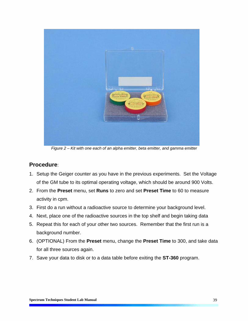
Radioactive Source (one each of an alpha, beta, and gamma sources – we
recommend Po-210, Sr-90, Co-60 respectively.) – shown in Figure 2.
Spectrum Techniques Student Lab Manual
39
Figure 2 – Kit with one each of an alpha emitter, beta emitter, and gamma emitter
Procedure:
1. Setup the Geiger counter as you have in the previous experiments. Set the Voltage
of the GM tube to its optimal operating voltage, which should be around 900 Volts.
2. From the Preset menu, set Runs to zero and set Preset Time to 60 to measure
activity in cpm.
3. First do a run without a radioactive source to determine your background level.
4. Next, place one of the radioactive sources in the top shelf and begin taking data
5. Repeat this for each of your other two sources. Remember that the first run is a
background number.
6. (OPTIONAL) From the Preset menu, change the Preset Time to 300, and take data
for all three sources again.
7. Save your data to disk or to a data table before exiting the ST-360 program.

Spectrum Techniques Student Lab Manual
40
Data Analysis:
1. Open Microsoft Excel® and import your data into it.
2. In cell E2 enter constant, K = and in cell F2 enter 2.20E6 (or 0.00000220). In cell E3
enter (conversion from Ci to dpm). (To create the , you need to change to the
Symbol font and then simply type the letter m. Don’t forget to switch back to your
original font when you are done.)
3. In cell E5 enter Dead Time = and in cell F6 enter the dead time for your GM tube
found in Lab #4: Resolving Time.
4. In cell G10, enter Activity (Ci). Then cells G13-G17, enter the activities of the
sources used. (Remember to not enter one for the background counts row.)
5. In cell H9 enter Res. Corr. and in cell H10 enter Counts. In cell C13, enter the
formula to correct for resolving time. Copy this formula to cells C14 and C15. Then,
in cell H16, enter the formula again and copy to cells H17 and H18. This should
change the five minute counts to counts per minute, and corrects them for resolving
time.
6. In cell I9 enter Bkgd Corr. and in cell I10 enter Counts. In cell I13, enter the
formula =H13-$C$12. Copy this formula to the other cells. (You may have to adjust
the formula if you took a five minute background count, but don’t forget to convert it
to cpm by dividing by 5.)
7. In cell J10, enter % efficiency. In cell J13, enter the formula for efficiency and copy
it to all the relevant cells.
8. Copy your results to your data table or print out a hard copy if you need to hand one
in attached to a lab report
Conclusions:
Are your results reasonable? How do you know? You should have numbers
above zero but below 10 if you performed the experiment correctly. Answer the post-
lab questions to help you form a conclusion from your results.

Spectrum Techniques Student Lab Manual
41
Post-Lab Questions:
1. Is the efficiency you calculated for each isotope valid only for that isotope?
Explain your answer.
2. If a different shelf is used, will the efficiency change? Explain your answer.
3. The radius of the GM tube’s window is 3.5 cm. The source is 3 cm from the
GM tube. Compare the surface area of a sphere 3 cm from the source to the
area of the GM tube’s window. (Hint: find the ratio) How is this related to this
experiment? Can this tell you if your results are reasonable?
4. (Correlates if five minute and one minute runs were taken.) Are the
efficiencies different? How different? Why?

Spectrum Techniques Student Lab Manual
42
Data Sheet for GM Tube Efficiency Lab
Tube #: Run Duration:
Dead Time: (Time)
Source Counts Corr. Counts Expect. Counts Efficiency
Tube #: Run Duration:
Dead Time: (Time)
Source Counts Corr. Counts Expect. Counts Efficiency
Name: Lab Session: Date: Partner:

Spectrum Techniques Student Lab Manual
43
Lab #6: Shelf Ratios
Objective:
The student will investigate the relationship between the distance and intensity of
radiation. The student will also measure the shelf ratios of the sample holder.
Pre-lab Questions:
1. Does radiation gain intensity or lose intensity as a source gets farther from a
detector?
2. How is radiation emitted from a radioactive source? (Hint: Think of the sun)
Introduction:
Although radiation is emitted from a source in all directions, only a small part
actually enters the tube to be counted. This fraction is a function of the distance, h,
from the point source of radiation to the GM tube. See Figure 1 for a picture of a
“sphere” which represents the radiation emitted radially from the radioactive source. It
can also be observed the small fraction of the “sphere” that will enter the window of
Geiger counter, which is represented by the triangle of sides d and height h. If the
source is moved further away from the tube, the amount of radiation entering the tube
should decrease. This is due to the fact that the triangle’s height will increase, and the
triangle will represent less and less of the “sphere” of radiation.

Spectrum Techniques Student Lab Manual
44
Figure 1: Influence of the source-to-window
distance on the observed count rate.
As a beta source is moved away from the detector, activity will decrease more
rapidly than predicted by the inverse square law because beta particles are also
attenuated or absorbed by air. The problem presented by this extra absorption is
placing the source close enough to get a good fraction of the radiation in the window of
the GM tube, but also not placing the source too far away where absorption becomes a
important factor to consider.
It is sometimes convenient to take advantage of this change in activity with
distance by moving less active samples toward the counter and samples which are too
active away from the tube in order to obtain suitable counting rates. This is the reason
that tube stands are made with multiple shelves.

Spectrum Techniques Student Lab Manual
45
Equipment:
Set-up for ST-360 Counter with GM Tube and stand (Counter box, power
supply – transformer, GM Tube, shelf stand, USB cable, and a source holder
for the stand) – shown in Figure 1.
Figure 1 – Setup for ST360 with sources and absorber kit
Radioactive Source (beta sources – we recommend Tl-204 or Sr-90) – green
source in Figure 1.
Procedure:
1. Setup the Geiger counter as you have in the previous experiments. Set the Voltage
of the GM tube to its optimal operating voltage, which should be around 900 Volts.
2. From the Preset menu, set Runs to zero and set Preset Time to 30.
3. First do a run without a radioactive source to determine your background level.
4. Next, place the radioactive source in the top shelf and begin taking data. In this
position, the source is 2 cm from the GM tube’s actual detector components.

Spectrum Techniques Student Lab Manual
46
5. Move the source down one shelf each time and take another run. You should see
the data accumulating in the Data window. After all ten shelves have been used,
save the data onto disk or record in a data table. Remember that the first run is a
background number.
Data Analysis:
1. Open Microsoft Excel® and import your data into it.
2. In Cell E2 enter Dead Time = and in cell F2 enter the dead time for your GM tube
(found in Lab #4).
3. In cell G9 enter Res. Corr. and in cell G10 enter Counts. In cell G13, enter the
formula to correct for resolving, or dead, time and copy this to the rest of the cells
corresponding to counts in column C.
4. In cell H9 enter Bkgd Corr. and in cell H10 enter Counts. In cell H13, enter the
formula to correct for the background, and copy this to the rest of the cells
corresponding to counts in column G.
5. In cell I9 enter Shelf and in cell I10 enter Ratio. In cell I13, enter the formula to
compute the shelf ratio, and copy this to the rest of the cells corresponding to counts
in column H. The shelf ratio is calculated by dividing the number of counts on any
shelf by the number of counts from the second shelf. This should give you a shelf
ratio of 1.00 for the second shelf, which is our reference point.
Conclusions:
You should see a decrease in your values as you move away from the source. If
you do not, this may be caused by statistical fluctuations in your counts. Why?
Post-Lab Questions:
1. Does the shelf ratio depend on the identity of the sample used?
2. If the experiment is repeated with a gamma or alpha source, what differences
would you expect?
3. Why is the second shelf the reference shelf?

Spectrum Techniques Student Lab Manual
47
Data Sheet for Shelf Ratios Lab
Tube #: Run Duration:
Dead Time:
(Time)
Shelf # Counts Corr. Counts Shelf Ratio
1
2 1.00
3
4
5
6
7
8
9
10
Name: Lab Session: Date: Partner:
Spectrum Techniques Student Lab Manual
48
Lab #7: Backscattering
Objective:
The student will investigate the relationship between absorber material (atomic
number) and backscattering in Part One. In Part Two, the student will investigate the
relationship between absorber thickness and backscattering
Pre-lab Questions:
1. Calculate what percentage of the entire “sphere” surrounding the source does the
GM window occupy.
2. Backscattering does have dependencies on atomic number and on thickness. Does
either one dominant the amount of backscattering versus the other? What kind of
dependence do you predict for each (direct, inverse, inverse square for example –
be descriptive)?
Introduction:
Radiation is emitted from a source in all directions. The radiation emitted within
the angle subtended by the window of the GM tube is the only radiation counted. Most
radiation is emitted away from the tube but it strikes matter. When it does so, the
direction of its path may be deflected. This deflection is known as scattering. Most
particles undergo multiple scattering passing through matter. Beta particles especially
may be scattered through large angles. Radiation scattered through approximately
1800 is said to be backscattered. For Geiger counters, backscatter is the fraction of
radiation emitted away from the GM tube that strikes the material supporting the
sample. It is deflected toward the tube window and is counted.
A beta particle entering matter undergoes a series of collisions with mostly nuclei
and sometimes orbital electrons. A collision between particles does not occur in the
same manner we picture them in the macroscopic world. There are very little contact
collisions, but instead the term, collision, refers to any interaction, coulombic or
otherwise. (A coulombic interaction is an electrical attraction or repulsion that changes
the path of the particle’s motion.) A collision may be elastic or inelastic, but in either

Spectrum Techniques Student Lab Manual
49
case the result is not only a change in direction but usually a decrease in the energy of
the beta particle as well (inelastic).
In the first part of the experiment, we will investigate the effect of the size of the
nucleus on backscattering since this would seem most likely effect the number of
backscattered beta particles. This can be determined by using absorbers as backing
materials. Even though the metal pieces you will use are called absorbers, in this
experiment, they will also be used to deflect radiation upward into the GM tube. To
eliminate any other effects, the absorbers will be the same thickness but different
atomic number (and thus different sized nuclei). In the second part of the experiment,
you will use absorbers of the same material (atomic number) and different thickness.
This is a common experimental technique, fixing one variable and varying another to
investigate each one individually
Normally when we think of thickness, we think of linear thickness that can be
measured in a linear unit such as inches or centimeters. However, in nuclear and
particle physics, thickness refers to areal thickness. This is the thickness of the
absorbers in mg/cm2. The absorptive power of a material is dependent on its density
and thickness, so the product of these two quantities is given as the total absorber
thickness, or areal thickness. We determine areal thickness with the equation:
Density (mg/cm3) X thickness (cm) = Absorber thickness (mg/cm2). (1)
You will determine the dependence that absorber thickness has on backscattering.
Equipment:
Set-up for ST-360 Counter with GM Tube and stand (Counter box, power
supply – transformer, GM Tube, shelf stand, USB cable, and a source holder
for the stand)
Spectrum Techniques Student Lab Manual
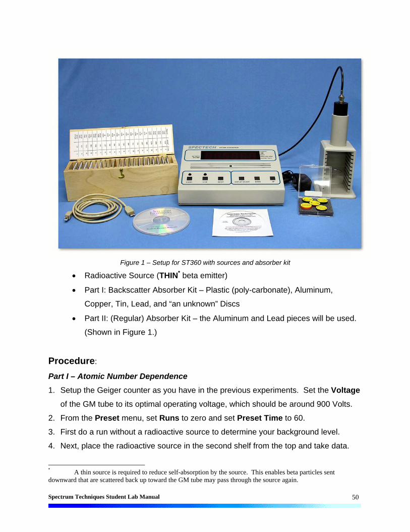
50
Figure 1 – Setup for ST360 with sources and absorber kit
Radioactive Source (THIN* beta emitter)
Part I: Backscatter Absorber Kit – Plastic (poly-carbonate), Aluminum,
Copper, Tin, Lead, and “an unknown” Discs
Part II: (Regular) Absorber Kit – the Aluminum and Lead pieces will be used.
(Shown in Figure 1.)
Procedure:
Part I – Atomic Number Dependence
1. Setup the Geiger counter as you have in the previous experiments. Set the Voltage
of the GM tube to its optimal operating voltage, which should be around 900 Volts.
2. From the Preset menu, set Runs to zero and set Preset Time to 60.
3. First do a run without a radioactive source to determine your background level.
4. Next, place the radioactive source in the second shelf from the top and take data.
* A thin source is required to reduce self-absorption by the source. This enables beta particles sent downward that are scattered back up toward the GM tube may pass through the source again.
Spectrum Techniques Student Lab Manual
51
5. Place an absorber piece, or disk, in the source holder and place the source directly
on top of it.
6. Repeat this for all of the various absorbers (different materials) including the
unknown.
7. Record the data to a file on disk or into a data table.
Part II – Thickness Dependence
1. Setup the Geiger counter as you have in the previous experiments. Set the Voltage
of the GM tube to its optimal operating voltage, which should be around 900 Volts.
2. From the Preset menu, set Runs to zero and set Preset Time to 60.
3. First do a run without a radioactive source to determine your background level. (Do
not repeat if this is part is being performed in the same lab period as Part I.)
4. Next, place the radioactive source in the second shelf from the top and begin taking
data.
5. Place the source directly on top of one of the absorbers. Take data by clicking on
the green diamond.
6. Place the source on a different absorber and insert into the second shelf. Click on
the green diamond to begin taking data.
7. Repeat for at least three other absorber thicknesses.
8. Record the data to a file on disk or into a data table.
Data Analysis:
Part I – Atomic Number Dependence
1. Open Microsoft Excel® and import your data into it.
2. In cell E2, enter Dead Time = and in cell F2 enter the dead time determined for your
GM tube.
3. In cell G9 enter Dead Corr. and in cell G10 enter Counts. In cell G13, enter a
formula to correct for dead time. Copy this down for the cells that have counts in
column C.
4. In cell H9 enter Corrected and in cell H10 enter Counts. In cell H13, enter a
formula to correct for background counts. Copy this down for the cells that have

Spectrum Techniques Student Lab Manual
52
counts in column G. Is background significant? Can you back up your answer
numerically?
5. In cell I9 enter Atomic and in cell I10 enter Number. In cell I13 and below, enter the
atomic numbers for the absorbers you used to get obtain the corresponding counts.
(Plastic is poly-carbonate** – Z = 6, Aluminum – Z = 13, Copper – Z = 29, Tin – Z =
50, and Lead – Z = 82)
6. To double-check the general result of our data that we will graph below, we will
calculate the percentage of counts that were due to backscattering and compare that
to the Z values. To calculate the percent of counts from backscattering, use the
following formula 100%
o
o
r
rrback , where r is the corrected count rate (cpm)
and ro is the count rate without any absorber present. To do this in Excel, in cell J9
enter Percent and cell J10 Backscatt. In cell J13, enter the formula
=((H13-$H$13)/$H$13)*100. This should give 0 for cell J13 but not for the rest.
7. Next, make a graph of Corrected Counts vs. Atomic Number. Start with the Chart
Wizard either by choosing Chart from the Insert Menu or pressing its icon on the top
toolbar.
9. Select the Atomic Number values in the I column and Corrected Counts values in
the H column.
10. Fill in the Chart Title, Value (X) Axis, and Value (Y) Axis windows with appropriate
names and units (if applicable) for those items.
11. Choose whether you want to view your graph as a separate worksheet as your data,
or you wish to see a smaller version of the graph with the data.
12. Adjust the size of the graph for your preference (or the instructor’s). You may also
wish to adjust the scales on one or more of the axes. Again, this is a preference
issue.
13. Right click on one of the data points and from the menu that appears, choose Add
Trendline. Make sure that the Linear option is chosen (should be darkened). Then
click on the Options tab and check the boxes for Display equation on chart and
* * Plastic is effectively carbon because that is the dominating element in this material.

Spectrum Techniques Student Lab Manual
53
Display R-squared value on chart. This will make the equation of the best fit line
appear as well as a number that represents the percent of linearity of the data.
Part II – Thickness Dependence
1. Open Microsoft Excel® and import
2. In cell E2, enter Dead Time = and in cell F2 enter the dead time determined for your
GM tube.
8. In cell G9 enter Dead Corr. and in cell G10 enter Counts. In cell G13, enter a
formula to correct for dead time. Copy this down for the cells that have counts in
column C.
9. In cell H9 enter Corrected and in cell H10 enter Counts. In cell H13, enter a
formula to correct for background counts. Copy this down for the cells that have
counts in column G.
3. In cell I9 enter Thickness and in cell I10 enter (in). In cell I13 and below, enter the
thickness of the absorbers (0.32, 0.063, or 0.125 inches) for the aluminum and
lead***.
4. Calculate the percentage of counts that were due to backscattering. In cell J9 enter
Percent and cell J10 Backscatt. In cell J13, enter the same formula as for Part I for
percent of backscattering. This should give 0 for cell J13 but not for the rest.
5. Next, make a graph of Corrected Counts vs. Thickness. Start with the Chart Wizard
either by choosing Chart from the Insert Menu or pressing its icon on the top toolbar.
6. Select the Thickness values in the I column and Corrected Counts values in the H
column.
7. Fill in the Chart Title, Value (X) Axis, and Value (Y) Axis windows with appropriate
names and units (if applicable) for those items.
8. Choose whether you want to view your graph as a separate worksheet as your data,
or you wish to see a smaller version of the graph with the data.
* ** Lead has an absorber that is 0.064 inches thick instead of the listed 0.063 inches. Make sure you enter it correctly.

Spectrum Techniques Student Lab Manual
54
9. Adjust the size of the graph for your preference (or the instructor’s). You may also
wish to adjust the scales on one or more of the axes. Again, this is a preference
issue.
10. Right click on one of the data points and from the menu that appears choose Add
Trendline. Make sure that the Linear option is chosen (should be darkened). Then
click on the Options tab and check the boxes for Display equation on chart and
Display R-squared value on chart. This will make the equation of the best-fit line
appear as well as a number that represents the percent of linearity of the data.
Conclusions:
What is your conclusion about the dependence of backscattering on atomic
number? How about on thickness?
Post-Lab Questions:
1. Justify your answers to the questions about the dependences of
backscattering.
2. Do your % backscattering calculations confirm your results?
3. What element (or material) is the unknown absorber?
4. What would be the predicted count rate for a uranium disk of the same size
as those used in Part I? How about if it was ¼ in. thick (qualitative answer,
higher or lower)? Show your work and explain any reasoning.

Spectrum Techniques Student Lab Manual
55
Data Sheet for Backscattering Lab
Tube #: Run Duration:
Dead Time: (Time)
Part I
Element (Z) Counts Corr. Counts % Backscat.
Name: Lab Session: Date: Partner:
Name: Lab Session: Date: Partner:
Don’t forget to hand in a graph of the data with this table.

Spectrum Techniques Student Lab Manual
56
Data Sheet for Backscattering Lab
Tube #: Run Duration:
Dead Time: (Time)
Part II
Thickness Counts Corr. Counts % Backscat.
Don’t forget to hand in a graph of the data with this table.
Spectrum Techniques Student Lab Manual
57
Lab #8: Inverse Square Law
Objective:
The student will verify the inverse square relationship between the distance and
intensity of radiation.
Pre-lab Questions:
1. Write a general mathematical expression for an inverse square law.
2. What are other examples of inverse square laws?
Introduction:
As a source is moved away from the detector, the intensity, or amount of
detected radiation, decreases. You may have observed this effect in a previous
experiment, Shelf Ratios Lab. If not, you have observed a similar effect in your life.
The farther you move away from a friend, the harder it is to hear them. Or the farther
you move away from a light source, the harder it is to see. Basically, nature provides
many examples (including light, sound, and radiation) that follow an inverse square law.
What an inverse square law says is that as you double the distance between
source and detector, intensity goes down by a factor of four. If you triple the distance,
intensity would decrease by a factor of nine. If you quadruple the distance, the intensity
would decrease by a factor of 16, and so on and so on. As a result, if you move to a
distance d away from the window of the GM counter, then the intensity of radiation
decreases by a factor 1/d2.
Equipment:
Set-up for ST-360 Counter with GM Tube and stand (Counter box, power
supply – transformer, GM Tube, shelf stand, USB cable, and a source holder
for the stand) – shown in Figure 1.

Spectrum Techniques Student Lab Manual
58
Figure 1 – Setup for ST360 with sources and absorber kit
Radioactive Source (beta sources – we recommend Tl-204 or Sr-90) – one of
the green sources shown in Figure 1.
Procedure:
1. Setup the Geiger counter as you have in the previous experiments. Set the Voltage
of the GM tube to its optimal operating voltage, which should be around 900 Volts.
2. From the Preset menu, set Runs to zero and set Preset Time to 30.
3. First do a run without a radioactive source to determine your background level.
4. Next, place the radioactive source in the top shelf and begin taking data. In this
position, the source is 2 cm from the GM tube’s actual detector components.
5. Move the source down one shelf each time and take another run. You should see
the data accumulating in the Data window. After all ten shelves have been used,
save the data onto disk or record in a data table. Remember that the first run is a
background number.
Data Analysis:

Spectrum Techniques Student Lab Manual
59
1. Open Microsoft Excel® and import your data into it.
2. In cell E2, enter Dead Time = and in cell F2 enter the dead time determined for your
GM tube.
3. Go cell G9 and insert the word True. Go to cell G10 and insert the word Counts. In
cell H10, insert Distance (cm). In cell I10, insert Distance (m). In cell J10, insert
1/d^21.
4. In cells G13 down to G14, insert a formula to correct for dead time and background.
(may need additional column).
5. In cell H13, insert the distances in centimeters. They should begin with 2 and
increase by one until 11 is reached.
6. In cell I13, insert the formula to convert the distance from centimeters to meters.
Copy this formula in each cell from I14 down to I22.
7. In cell J13, insert the formula =1/(I13*I13) or =1/(I13^2). Either form gets you the
inverse square of the distance. Copy this formula in the cells down from J14 to J22.
8. Next, make a graph of Counts vs. 1/d2. Start with the Chart Wizard either by
choosing Chart from the Insert Menu or pressing its icon on the top toolbar.
9. Choose the True Counts values in the H column and the 1/d2 values in the J column.
10. Fill in the Chart Title, Value (X) Axis, and Value (Y) Axis windows with appropriate
names and units (if applicable) for those items. Recall that Counts are a unitless
quantity.
11. Position your cursor directly over one of the data points on your graph. Then click
the right button on the mouse and watch a small menu appear. Choose the Add
Trendline option. You may click OK here or if you want more information choose
the Options Tab. There you may click in the boxes for Display Equation on Chart
(for the equation of the line in slope-intercept form to appear on the graph) or on
Display R-squared Value on Chart (this gives a decimal representation of the
percentage completely linear the data is).
Conclusions:
Use your graph to determine if the data does indeed obey inverse square law.
1 The carrot, ^, is the computer programming way of indicating exponent or power.

Spectrum Techniques Student Lab Manual
60
Post-Lab Questions:
1. Does your data follow Excel®’s best fit line? If not, why?
2. Does this verify the inverse square law? Explain?

Spectrum Techniques Student Lab Manual
61
Data Sheet for Inverse Square Law Lab
Tube #: Run Duration:
Dead Time: (Time)
Counts Corr. Counts Distance 1/d^2
Counts Corr. Counts Distance 1/d^2
Name: Lab Session: Date: Partner:
Don’t forget to hand in a graph of the data with this table.
Spectrum Techniques Student Lab Manual
62
Lab #9: Range of Alpha Particles
Objective:
The student will determine the range of an alpha particle in air, and consequently
the alpha particle’s energy.
Pre-lab Questions:
1. What is an alpha particle? How and why are they emitted?
2. What everyday material can block alpha particles?
3. Do you predict the range to be long or short? Why?
Introduction:
We know that particles that enter matter lose their energy1 via collisions with
atoms in the matter. So, a natural question would be, how far will the particle travel in
the matter before it loses all of its energy? This quantity is called the range of a
particle, and depends on the type of material, particle type, and its energy. Normally,
we assume that the energy loss is continuous (particle loses some energy for each
amount of distance it travels); the range will be a certain distance for the same particles
with identical initial energies passing through the same type of material. In this
experiment, you will look at alpha particles passing through air.
The alpha particle () is a helium ion (+2), which is composed of two protons (p)
and two neutrons (n). Ramsay and Soddy observed that helium is constantly being
produced from radium and that radioactive minerals invariably contain helium.
Rutherford and Royds later showed that alpha particles form neutral helium atoms when
they lose their kinetic energy. In the process, each alpha particle gains two electrons
from the surrounding material.
Alpha particles emitted from a particular species of nucleus are mono-energetic;
alphas from the same species have the same energy. The energy of most alphas falls
1 When dealing with particles, we ignore potential energies from bonding mainly because the size is so small. The term energy refers solely to the kinetic energy of the particle.

Spectrum Techniques Student Lab Manual
63
in the range between 3 and 8 MeV. By comparison, chemical reactions have energies
of 5 to 30 eV per molecule.
The velocity of an alpha particle upon emission from the nucleus depends upon
the radioelement of its origin. The alpha particle has great ionizing power, but very little
penetrating power. (If it enters the GM tube, then it will ionize the gas and be detected
unless it is the dead time.) Its energy is approximated by its range in air in the equation:
5.1 RE , (1)
where R is the range in air of the alpha particle in centimeters and E is the energy of the
alpha particle in MeV.
Equipment:
Set-up for ST-360 Counter with GM Tube and stand (Counter box, power
supply – transformer, GM Tube, shelf stand, USB cable, and a source holder
for the stand) – shown in Figure 1.
Figure 1 – Setup for ST360 with sources and absorber kit

Spectrum Techniques Student Lab Manual
64
Radioactive Source (alpha emitter – Po-210 is best for this experiment – the
red source shown in Figure 1)
Procedure:
1. Setup the Geiger counter as you have in the previous experiments. Set the Voltage
of the GM tube to it optimal operating voltage, which should be approximately 900
Volts.
2. From the Preset menu, set Runs to three and set Preset Time to 60. (You will take
three data sets from each shelf due to the low count rate on some shelves.)
3. First do a run without a radioactive source to determine your background level.
4. Next, place the radioactive source in the top shelf from the top and begin taking
data.
5. Move the source down one shelf and take data again.
6. Repeat this until you repeatedly get counts approximately equal to your background.
(This means you will take data until the source reaches the sixth or seventh shelf
approximately.)
7. Save your data either to disk or into a data table.
Data Analysis:
1. Open Microsoft Excel® and import your data into it.
2. In cell E2, enter Dead Time = and in cell F2 enter the dead time determined for your
GM tube.
3. In cell G9 enter Corrected and in cell G10 enter Counts. In cells G15, enter a
formula for dead time and background correction (average background runs first -
Cells C12-C14), and copy that formula down to cell G32.
4. Now, average the three runs you preformed on each of the shelves. In cell H9 enter
Average and in cell H10 enter Counts.
5. Next, add the distances to the chart. In cell J10, enter Distance (cm). Starting in
cell J13, enter 2. Then in cell J14, enter the formula =J13+1 and copy this down for
all the distances you took data.
Spectrum Techniques Student Lab Manual
65
6. Use that number as R in Equation (1) to find the energy of your alpha particles.
Compare this value of E to the expected value, 5.34 MeV, by finding the percent
error. Record these values either in the spreadsheet or on your data sheet.
100%
ltheoretica
ltheoreticameasurederror (2)
OPTIONAL:
7. A graph is very tricky here because of lack of measurements below 2 cm. In
addition, you would like measurements in increments less than 1 cm. Look at your
data. Where is there a sudden fall-off in the counts per minute (going from
thousands to tens)? Where does the data dip below the x-axis? Use extrapolation
to guess where these two situations occur (i.e., 2.7 cm because it fell in-between 2
cm and 3 cm but seems closer to 3 cm). Average these two numbers and that gives
the mean range of your alpha particles.
8. Make a graph of Corrected Counts per Minute vs. Distance. Start with the Chart
Wizard either by choosing Chart from the Insert Menu or pressing its icon on the
top toolbar.
9. Use the Average Counts in column I and Distance in column J columns of data.
10. Fill in the Chart Title, Value (X) Axis, and Value (Y) Axis windows with appropriate
names and units (if applicable) for those items.
11. Choose whether you want to view your graph as a separate worksheet as your data,
or you wish to see a smaller version of the graph with the data. Click Finish when
you have chosen one or the other.
Conclusions:
What you should see in a graph of your data (if you made one) is that as the data
approaches the range, it does not drop immediately to the background level directly at
the range value. Instead, the curve slopes down over a certain interval of distances.
This is because our original assumption of energy loss being continuous is not quite
accurate. Not every identical particle will have identical energy loss. That is because
every particle suffers a different number of collisions when passing through matter and
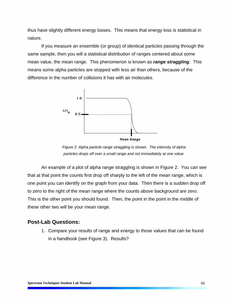
Spectrum Techniques Student Lab Manual
66
thus have slightly different energy losses. This means that energy loss is statistical in
nature.
If you measure an ensemble (or group) of identical particles passing through the
same sample, then you will a statistical distribution of ranges centered about some
mean value, the mean range. This phenomenon is known as range straggling. This
means some alpha particles are stopped with less air than others, because of the
difference in the number of collisions it has with air molecules.
Figure 2: Alpha particle range straggling is shown. The intensity of alpha
particles drops off over a small range and not immediately at one value.
An example of a plot of alpha range straggling is shown in Figure 2. You can see
that at that point the counts first drop off sharply to the left of the mean range, which is
one point you can identify on the graph from your data. Then there is a sudden drop off
to zero to the right of the mean range where the counts above background are zero.
This is the other point you should found. Then, the point in the point in the middle of
these other two will be your mean range.
Post-Lab Questions:
1. Compare your results of range and energy to those values that can be found
in a handbook (see Figure 3). Results?

Spectrum Techniques Student Lab Manual
67
Figure 3: Plot of Alpha particle range versus energy in MeV.
2. How far away should a person stand to not receive any alpha particles that
are emitted from a nucleus at 8 MeV?
3. How reliable is your data? In other words, is the percent error high? (Explain
why you think it is high) If it is high, is that OK? Why?
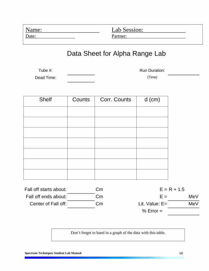
Spectrum Techniques Student Lab Manual
68
Data Sheet for Alpha Range Lab
Tube #: Run Duration:
Dead Time: (Time)
Shelf Counts Corr. Counts d (cm)
Fall off starts about: Cm E = R + 1.5
Fall off ends about: Cm E = MeV
Center of Fall off: Cm Lit. Value: E= MeV
% Error =
Name: Lab Session: Date: Partner:
Don’t forget to hand in a graph of the data with this table.

Spectrum Techniques Student Lab Manual
69
Lab #10: Absorption of Beta Particles
Objective:
The student will investigate the attenuation of radiation via the absorption of beta
particles.
Pre-lab Questions:
1. How does activity of a source vary with distance?
2. How do you predict activity will vary with increasing absorber thickness, when an
absorber is placed between the source and window of the GM tube?
Introduction:
Beta particles are electrons that are emitted from an atom when a neutron
decays by the weak force. The neutron (n) becomes a proton (p), an electron (e-), and
an anti-neutrino ( )1. When an electron originates in the nucleus, it is called a beta
particle.
epn (1)
Unlike alpha particles that are emitted from the nucleus with the same energy (~5
MeV), beta particles are emitted with a range of energies between 0 MeV and the
maximum energy for a given radioactive isotope. The velocity of a beta particle is
dependent on its energy, and velocities range from zero to about 2.9 x 10⁸ m/s, nearly
the speed of light. So the beta particles do not all have the same kinetic energy and
thus they do not all have the same range. When the range varies over different values,
this is called range straggling. It represents the different energy losses all of the beta
particles have given their different initial values. Figure 1 shows a typical absorption
curve for beta particles, which illustrates the range straggling.
1 The purpose of the anti-neutrino’s creation is to carry off extra energy and momentum for the conservation of those quantities.
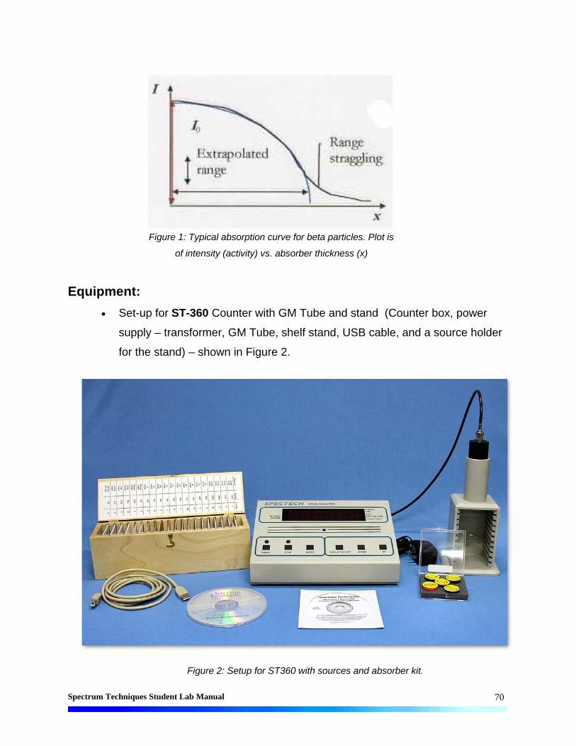
Spectrum Techniques Student Lab Manual
70
Figure 1: Typical absorption curve for beta particles. Plot is
of intensity (activity) vs. absorber thickness (x)
Equipment:
Set-up for ST-360 Counter with GM Tube and stand (Counter box, power
supply – transformer, GM Tube, shelf stand, USB cable, and a source holder
for the stand) – shown in Figure 2.
Figure 2: Setup for ST360 with sources and absorber kit.

Spectrum Techniques Student Lab Manual
71
Radioactive Source (beta emitter – any green source shown in Figure 2)
Procedure:
1. Setup the Geiger counter as you have in previous experiments. Set the Voltage of
the GM tube to its optimal operating voltage, which should be around 900 Volts.
2. From the Preset menu, set Runs to zero and set Preset Time to 60.
3. First do a run without a radioactive source to determine your background level.
4. Next, place the radioactive source in the second shelf from the top and begin taking
data.
5. Place an absorber piece in the top shelf and take another run of data.
6. Repeat this a minimum of 5 more times with absorbers of increasing thickness.
Data Analysis:
1. Open Microsoft Excel® and import your data into it.
2. In cell F6, enter Dead Time = and in cell G6 enter the dead time determined for your
GM tube.
3. In cell G9, enter Thickness and in cell G10 enter mg/cm2. Then starting in cell
G13, enter the thickness for the absorbers used. For cell G13, it should be zero (no
absorber used). In column F, under Notes, it may be convenient to enter the letters
associated with the absorbers you used.
4. In cell H9 enter Dead Corr. and in cell H10 enter Counts. Then starting in cell H13,
enter a formula to correct for the dead time of the GM counter. Copy this formula
down the column for all the data you collected.
5. In cell I9 enter Corrected and in cell I10 enter Counts. Then starting in cell I13,
enter a formula to correct for the background of the GM counter. Copy this formula
down for all the data you have.
6. In cell J9 enter Natural Log and in cell J10, enter of Counts. Then in cell J13, enter
the formula =LN(I13) and copy this formula down for all the data you have.
7. Next, make a graph of Corrected Counts vs. Thickness. Start with the Chart
Wizard either by choosing Chart from the Insert Menu or pressing its icon on the
top toolbar.

Spectrum Techniques Student Lab Manual
72
8. Select the Thickness values in the G column and the Corrected Counts values in
the I column.
9. Fill in the Chart Title, Value (X) Axis, and Value (Y) Axis windows with appropriate
names and units (if applicable) for those items.
10. Add a trendline to the graph. The x-intercept represents the extrapolated range.
Conclusions:
You should be able to characterize the relationship between beta particle activity
and absorber thickness.
Post-Lab Questions:
1. Is your data linear? If not, what type of behavior does it exhibit?
2. What is the slope for your data? How did you obtain it?
3. What is the range of the beta particles, so that all of them stop?
4. Bremmsstrahlung (German for braking radiation) is the name given to x-rays
produced by beta particles reacting with matter. Was any Bremmsstrahlung
produced during the experiment? Can it minimized?

Spectrum Techniques Student Lab Manual
73
Data Sheet for Beta Absorption Lab
Tube #: Run Duration:
Dead Time: (Time)
Counts Corr. Counts Thickness ln (Counts)
Name: Lab Session: Date: Partner:
Don’t forget to hand in a graph of the data with this table.

Spectrum Techniques Student Lab Manual
74
Lab #11: Beta Decay Energy
Objective:
The student will determine the maximum energy of decay of a beta particle.
Pre-lab Questions:
1. What is the decay mechanism for beta decay? Why are there three decay
products?
2. What are the units of thickness for an absorber?
3. Why shouldn’t a beta source be placed below the third shelf? Or above the second
shelf?
Introduction:
When beta particles are emitted from a nucleus, they are emitted over a wide
range of energies. Recall that this is different from alpha particles, which are emitted
monoenergetically. The maximum energy of the emitted beta particles is a
characteristic signature for different radioisotopes.
In this experiment, you will find the range of beta particles by measuring their
attenuation1 with absorbers and extrapolating the absorption curve. The range R will
then be substituted into the formula
212.084.1 RE (1)
where R is in g/cm2. (Note that the units for R are not the same as the absorber
thicknesses. You must convert at the end.) See Figure 1 for an example of an energy
curve for beta particles.
1 Attenuation is a term used for the exponential decrease of a quantity.

Spectrum Techniques Student Lab Manual
75
Figure 1: Typical plot of beta particle energy curve.
The spectrum is not linear and “tails” off at high energy, which means that there
are very few beta particles (This effect is seen with the phenomenon of range
straggling, which was observed in the absorption curve in the previous experiment.)
The reason is that most of the beta particles cannot penetrate the absorber and most of
the counts are background counts. Thus, one must assume linearity and extrapolate
the line to the x-axis. There are two options to finding this x-intercept. The first is to find
an equation for the best-fit line of the data in slope-intercept form, y = mx + b. Then set
y = 0 and solve for the x value, since the x-intercept is the point on the line where the y
– coordinate is zero. The second method is to take a copy of the plot and use a rule to
continue the linear part of the data through the x-axis and finding that point.
Equipment:
Set-up for ST-360 Counter with GM Tube and stand (Counter box, power
supply – transformer, GM Tube, shelf stand, USB cable, and a source holder
for the stand) – shown in Figure 2.
Radioactive Source (beta sources – Sr-90 or Tl-204 are recommended) –
green source shown in Figure 2.

Spectrum Techniques Student Lab Manual
76
Figure 2: Setup for ST360 with sources and absorber kit.
Procedure:
1. Set up the Geiger counter as you have in the previous experiments. Set the
Voltage of the GM tube to its optimal operating voltage, which should be around 900
Volts.
2. From the Preset menu, set Runs to three and set Preset Time to 60.
3. First do a run without any absorber and with a radioactive source. Place the source
in the second shelf and click the green diamond to begin taking data. No
background reading is taken because 204Tl and 90Sr are relatively strong beta
sources (high count rates) and the background will be negligible (20-40 cpm).
4. Next, place the first absorber in the top shelf, directly above the source, and begin
taking data.
5. Change your absorber each time for as many absorbers as the instructor gives to
you. You should see the data accumulating in the Data window. After all the
absorbers have been used, save the data onto disk or record in a data table.

Spectrum Techniques Student Lab Manual
77
Data Analysis:
1. Open Microsoft Excel® and import your data into it.
2. In cell E2 enter Dead Time = and then in cell F2 enter the value for your GM tube’s
resolving time.
3. In cell G9 enter Corrected and in cell G10 enter Counts. Next, in cell G13, enter a
formula to correct for your data for resolving time. Copy this formula down for all the
cells that should contain data.
4. In cell H9 enter Thickness and in cell H10 enter (mg/cm2). Then, in column H
beginning with cell 12, enter the thickness values you used taking data.
5. In cell I9 enter Log of and in cell I10 enter Activity. Next, in cell I13, enter the
formula =LOG(G13) to calculate the logarithm (base 10) of your data. Copy this
formula down for all the cells that should contain data. Taking the logarithm of the
data substitutes for plotting your data on semi-log paper.
6. Next, make a graph of Log of Activity vs. Thickness. Start with the Chart Wizard
either by choosing Chart from the Insert Menu or pressing its icon on the top toolbar.
7. Select the thickness values in the H column and the Log of Activity values in the I
column.
8. Fill in the Chart Title, Value (X) Axis, and Value (Y) Axis windows with appropriate
names and units (if applicable) for those items.
9. Add a trendline to your graph.
10. In cell A34, copy the equation shown for the best-fit line in your graph. Then, set y =
0 and solve for x. This breaks down to dividing the negative of the y-intercept by the
value for the slope (should be negative). Take the value for x and divide it by 1000,
because your answer was in mg/cm2. But to use the equation given earlier for
maximum energy, you need x in units of g/cm2. This is your value of the range R of
a beta particle emitted from your source.
11. Then plug your value for R into 212.084.1 RE and get a value for E. Place this
value in cell B36. In cell A36, enter E =.
12. In cell A38 enter True Value for E =. Then in cell B38, enter the literature value for
your source. (Sr-90 has E = 0.546 MeV and Tl-204 has E = 0.7634 MeV.)

Spectrum Techniques Student Lab Manual
78
13. In cell A40 enter Percent Error =. In cell B40, enter the formula =((ABS(B36-
B38))/B38)*100. This formula represents the formula
100%
true
measuredtrueerror . (2)
Conclusions:
You should have found the value for the maximum energy of a beta particle from
your source and the percent error of this result when compared to the literature value.
However, this percent error is not a good way to determine experimental error. As
discussed in a previous lab, the best way to determine error is to use the standard
deviation. So, calculate for your value of E – you will have to use propagation of
errors. (OPTIONAL)
Post-Lab Questions:
1. Does your data follow Excel’s® best fit line? If not, why?
2. Why does the data fluctuate so much at high absorber values, especially
those above 1400 mg/cm2? How can this be handled in the data analysis
stage?
3. Is your result for E accurate? Is it still a good result even if it is not exactly the
same as the literature value?

Spectrum Techniques Student Lab Manual
79
Data Sheet for Beta Energy Lab
Tube #: Run Duration:
Dead Time: (Time)
Counts Corr. Counts Thickness ln (Counts)
Equation for line: y=
For y=0, x= mg/cm^2
Conversion x= g/cm^2 (This is the range)
Use E = 1.84*R+0.212
E= MeV
Name: Lab Session: Date: Partner:
Don’t forget to hand in a graph of the data with this table.

Spectrum Techniques Student Lab Manual
80
Lab #12: Absorption of Gamma Rays
Objective:
The student will investigate the attenuation of radiation via the absorption of
gamma rays.
Pre-lab Questions:
1. How do gamma rays interact with matter (hint: there are three)?
2. Where are gamma rays on the electromagnetic spectrum? What are the
characteristics (high, low, short, or long) of their wavelength, frequency, and
energy?
3. How do you calculate mass thickness (g/cm2) from other quantities of a material?
Introduction:
Gamma radiation unlike alpha and beta radiation, consists of electromagnetic
waves. Gamma rays are emitted as photons, or little “packages” of energy called
quanta, which travel at the speed of light (c = 3.0 x 10⁸ m/s1). What differentiates
gamma rays, x-rays, visible light, and radio waves is their position in the
electromagnetic spectrum (see Figure 1). What actually happens is that some of these
“zones” actually overlap, especially between x-rays and gamma rays. While this is not
shown in explicitly in Figure 1, you can see that the x-rays and gamma rays do reside
next to one another on the spectrum.
1 A unit conversion shows that 3.0 x 10⁸ m/s = 30 cm/ns. That means in one nanosecond light travels 30 cm or in one second light travels 30 billion centimeters.

Spectrum Techniques Student Lab Manual
81
Figure 1: The electromagnetic spectrum
One significant difference between x-rays and gamma rays is their origin. X-rays
are produced in the electron shells, while gamma rays are produced in the nucleus. X-
rays are created when electrons undergo a deceleration or jump to lower energy levels.
Gamma rays are created by energy transitions in the nucleus. In this experiment, we
are mostly concerned with gamma rays, because any x-rays present will be shielded by
air and matter acting as absorbers.
When a beam of gamma rays impinges on a sheet of absorbing material, some
of the radiation will be absorbed or scattered2. As the thickness of the absorber is
increased, the fraction of the radiation passing through will decrease. When exactly half
the radiation passes through the absorber (and the other half is absorbed or scattered),
the thickness of the absorber is called the half thickness, X1/2.
2 Gamma rays interact with matter in three ways: (1) photoelectric effect (ionization), (2) Compton effect, and (3) pair production (e+e-). Your instructor can explain more.

Spectrum Techniques Student Lab Manual
82
This thickness, X1/2, is not normally how we perceive thickness. We normally
consider it to be a distance possibly in cm. Here, thickness is short for mass
thickness. Why? Because the thickness of different materials represents different
amounts of matter (atoms). But a mass thickness is used to represent how much
matter is being passed through (regardless of whether it is air, aluminum, or lead). To
calculate mass thickness you simply multiply the density of the material (g/cm3) times its
length, or normal thickness, (cm) to get the mass thickness (g/cm2). The absorbers you
will use for this experiment have their thickness listed as mass thickness because that
quantity can be used to compare the plastic to lead absorbers.
Since the intensity of radiation is reduced by 50% by passing through one X1/2, it
will be reduced by another 50%, or only to 25% of the original intensity, in passing
through a second X1/2 of absorber. A linear relationship is obtained if the data are
plotted using semi log paper or if the logarithm of the activity is plotted as a function of
the absorber thickness.
The attenuation (or absorption and scattering) of gamma rays is exponential in
nature, which is shown by the equation:
XoeII (1)
where I is the intensity of the beam after passing through X amount of absorbing
material, Io is the original intensity, is the mass attenuation coefficient, and X is the
mass thickness. Since the intensity of the gamma rays is cut in half after passing
through X1/2, we can rewrite Equation 1 as
2/1
2
1 Xoo eII . (2)
The Io terms cancel giving
2/1
2
1 Xe , (3)
which can again be rewritten by taking the natural logarithm of both sides
2/12
1ln X
. (4)
Using the rules of exponents, we know that ln(1/2) = -ln(2), so that gives
2/1)2ln( X . (5)

Spectrum Techniques Student Lab Manual
83
One final rearrangement gives us a value of the mass attenuation coefficient
2/12/1
693.0)2ln(
XX . (6)
During your data analysis, you will find a value for X1/2, and thus one for .
Equipment:
Set-up for ST-360 Counter with GM Tube and stand (Counter box, power
supply – transformer, GM Tube, shelf stand, USB cable, and a source holder
for the stand) – shown in Figure 2.
Figure 2: Setup for ST360 with sources and absorber kit.
Radioactive Source (gamma ray emitter – any of the sources pictured in
Figure 3).

Spectrum Techniques Student Lab Manual
84
Figure 3: Kit of eight different gamma sources.
Procedure:
1. Setup the Geiger counter as you have in the previous experiments. Set the Voltage
of the GM tube to its optimal operating voltage, which should be around 900 Volts.
2. From the Preset menu, set Runs to zero and set Preset Time to 60.
3. First do a run without a radioactive source to determine your background level.
4. Next, place the radioactive source in the second shelf from the top and begin taking
data.
5. Place an absorber piece in the top shelf and take another run of data.
6. Repeat this a minimum of 5 more times with absorbers of increasing thickness.
Data Analysis:
1. Open Microsoft Excel® and import your data into it.
2. In cell E2, enter Dead Time = and in cell F2 enter the dead time determined for your
GM tube.
3. In cell G9, enter Thickness and in cell G10 enter mg/cm2. Then starting in cell
G13, enter the thickness for the absorbers used. For cell G13, it should be zero (no
absorber used). In column F, under Notes, it may be convenient to enter the letters
associated with the absorbers you used.

Spectrum Techniques Student Lab Manual
85
4. In cell H9 enter Dead Corr. and in cell H10 enter Counts. Then starting in cell H13,
enter a formula to correct for the dead time of the GM counter. Copy this formula
down the column for all the data you collected.
5. In cell I9 enter Corrected and in cell I10 enter Counts. Then starting in cell I13,
enter a formula to correct for the background of the GM counter. Copy this formula
down for all the data you have.
6. Next, make a graph of Corrected Counts per Minute vs. Thickness. Start with the
Chart Wizard either by choosing Chart from the Insert Menu or pressing its icon on
the top toolbar.
7. Select the Thickness values in the G column and the Corrected Counts values in
the I column.
8. Fill in the Chart Title, Value (X) Axis, and Value (Y) Axis windows with appropriate
names and units (if applicable) for those items.
9. Choose whether you want to view your graph as a separate worksheet as your data,
or you wish to see a smaller version of the graph with the data.
10. Right click on the y-axis of the graph and choose the Format Axis option. Then
choose the Scale Tab, and check the Logarithmic Scale option towards the
bottom.
11. Add a trendline to your data to obtain the equation of the best fit line through your
data.
Conclusions:
From your best-fit line equation, find the values for X1/2 and . Make sure your
answers are in the appropriate units (involving grams and centimeters).
Post-Lab Questions:
1. Is your data linear? If not, why?
2. Looking at your data and equating intensity and counts per minute, does your
result for X1/2 a correct approximation? (Does your result match the data?)
3. Can we be completely shielded from gamma rays? If not, then why bother?

Spectrum Techniques Student Lab Manual
86
4. Comparing your range for alpha particles, the absorption of beta particles,
and now the results for gamma rays, why are they different?

Spectrum Techniques Student Lab Manual
87
Data Sheet for Gamma Absorption Lab
Tube #: Run Duration:
Dead Time: (Time)
Counts Corr. Counts Thickness ln (Counts)
Equation for line: y=
mg/cm^2
OR g/cm^2
Calculate x_1/2 = ln(2)/
x_1/2 = g/cm^2
Name: Lab Session: Date: Partner:
Don’t forget to hand in a graph of the data with this table.

Spectrum Techniques Student Lab Manual
88
Lab #13: Half-Life of Ba-137m
Objective:
The student will measure the half-life of metastable Barium-137.
Pre-lab Questions:
1. Explain how you will obtain Ba-137m from the isotope generator.
2. Draw the decay diagram for the process you describe in #1.
3. If a Sr-90 source has a count rate of 7020 cpm today, when will it have a count rate
of 1404 cpm? The half-life of Sr-90 is 28.6 yrs. When will Po-210 reach 1404 cpm
from 7020 cpm (half-life for Po-210 is 138 days)?
4. If a Tl-204 source has 1.34 x 10²¹ atoms today. When will it have 1.675 x 10¹⁸
atoms? The half-life for Tl-204 is 3.78 years.
Introduction:
The decay of radioactive atoms occurs at a constant rate. There is no way to
slow it down by maybe refrigeration or to accelerate the process with heat. The rate of
decay is also a constant, fixed rate regardless of the amount of radioactive atoms
present. That is because there are only two choices for each atom, decay or don’t
decay. Thus, the amount of radioactive atoms we have on hand at any time is
undergoing a consistent, continuous change.
The change in the number of radioactive atoms is a very orderly process. If we
know the number of atoms present and their decay constant (probability of decay per
unit time), then we can calculate how many atoms will remain at any future time. This
can be written as the equation
tNNtN )( , (1)
where N(t) is the number of atoms that will be present at time t, N is the number of
atoms present currently, is the decay constant, and t is the elapsed time. If the
number of radioactive atoms remaining is plotted against time, curves like those in
Figure 1 can be obtained. The decay constant can be obtained from the slope of these
curves (discussed more below).
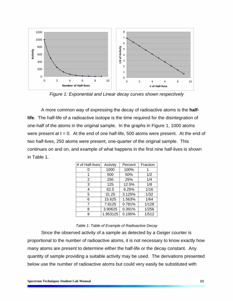
Spectrum Techniques Student Lab Manual
89
Figure 1: Exponential and Linear decay curves shown respectively
A more common way of expressing the decay of radioactive atoms is the half-
life. The half-life of a radioactive isotope is the time required for the disintegration of
one-half of the atoms in the original sample. In the graphs in Figure 1, 1000 atoms
were present at t = 0. At the end of one half-life, 500 atoms were present. At the end of
two half-lives, 250 atoms were present, one-quarter of the original sample. This
continues on and on, and example of what happens in the first nine half-lives is shown
in Table 1.
# of Half-lives Activity Percent Fraction 0 1000 100% 1 1 500 50% 1/2 2 250 25% 1/4 3 125 12.5% 1/8 4 62.5 6.25% 1/16 5 31.25 3.125% 1/32 6 15.625 1.563% 1/64 7 7.8125 0.781% 1/128 8 3.90625 0.391% 1/256 9 1.953125 0.195% 1/512
Table 1: Table of Example of Radioactive Decay
Since the observed activity of a sample as detected by a Geiger counter is
proportional to the number of radioactive atoms, it is not necessary to know exactly how
many atoms are present to determine either the half-life or the decay constant. Any
quantity of sample providing a suitable activity may be used. The derivations presented
below use the number of radioactive atoms but could very easily be substituted with
0
200
400
600
800
1000
1200
0 2 4 6 8 10
Number of Half-lives
Act
ivit
y
0
1
2
3
4
5
6
7
8
0 2 4 6 8 10
# of Half-lives
LN
of
Act
ivit
y
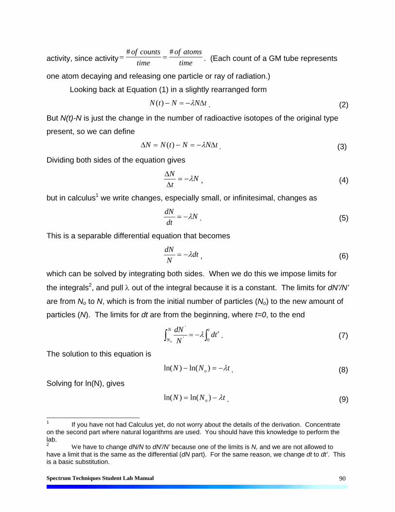
Spectrum Techniques Student Lab Manual
90
activity, since activitytime
atomsof
time
countsof ## . (Each count of a GM tube represents
one atom decaying and releasing one particle or ray of radiation.)
Looking back at Equation (1) in a slightly rearranged form
tNNtN )( . (2)
But N(t)-N is just the change in the number of radioactive isotopes of the original type
present, so we can define
tNNtNN )( . (3)
Dividing both sides of the equation gives
Nt
N
, (4)
but in calculus1 we write changes, especially small, or infinitesimal, changes as
Ndt
dN . (5)
This is a separable differential equation that becomes
dtN
dN , (6)
which can be solved by integrating both sides. When we do this we impose limits for
the integrals2, and pull out of the integral because it is a constant. The limits for dN’/N’
are from No to N, which is from the initial number of particles (No) to the new amount of
particles (N). The limits for dt are from the beginning, where t=0, to the end
tN
Ntd
N
dNo 0'
'
. (7)
The solution to this equation is
tNN o )ln()ln( . (8)
Solving for ln(N), gives
tNN o )ln()ln( . (9)
1 If you have not had Calculus yet, do not worry about the details of the derivation. Concentrate on the second part where natural logarithms are used. You should have this knowledge to perform the lab. 2 We have to change dN/N to dN'/N' because one of the limits is N, and we are not allowed to have a limit that is the same as the differential (dN part). For the same reason, we change dt to dt’. This is a basic substitution.

Spectrum Techniques Student Lab Manual
91
Thus, if we plot the natural log of the number of atoms (or activity) versus time, we will
get a straight line with slope = - and y-intercept = ln(No). This would allow us to find
the decay constant. Why?
We will need the decay constant in the next step, which is to find the half-life of
the radioactive isotope we are studying. Starting from Equation (8) and applying a
simple logarithmic identity, we get
tN
N
o
ln . (10)
If we are considering the half-life, then N is one-half of No (reduced ratio) and t is t1/2.
This changes our equation to be
2/12
1ln t
. (11)
Applying the reverse of our previous logarithmic identity, we get
2/1)2ln()1ln( t . (12)
The ln(1) = 0, so now we have
2/1)2ln( t . (13)
Finally, we can solve for the half-time
)2ln(
2/1 t . (14)
Equipment:
Set-up for ST-360 Counter with GM Tube and stand (Counter box, power
supply – transformer, GM Tube, shelf stand, USB cable, and a source holder
for the stand) – shown in Figure 2.

Spectrum Techniques Student Lab Manual
92
Figure 2: Setup for ST360 with sources and absorber kit.
Radioactive Source (Cs/Ba-137m Isotope Generator – shown in Figure 3)
Figure 3: Isotope Generator to make Ba-137m from Cs-137

Spectrum Techniques Student Lab Manual
93
Procedure:
1. Setup the Geiger counter as you have in the previous experiments. Set the Voltage
of the GM tube to its optimal operating voltage, which should be around 900 Volts.
2. From the Preset menu, set Runs to zero and set Preset Time to 30.
3. First do a run without a radioactive source to determine your background level.
4. Next, from the Preset menu, set the Runs to 31. (This will take 30 more runs so the
total number of runs is 31.)
5. From the isotope generator, obtain 10-12 drops of Ba-137m. Place the radioactive
source in the second shelf from the top and begin taking data.
6. Record the data to a file on disk or into a data table.
7. You may wish to do a second trial if time allows.
Data Analysis:
1. Open Microsoft Excel® and import your data into it.
2. In cell E2, enter Dead Time = and in cell F2 enter the dead time determined for your
GM tube.
3. In cell G9 enter Dead Corr. and in cell G10 enter Counts. In cell G13, enter a
formula to correct for resolving time and copy it down for the cells that have counts
in column C.
4. In cell H9 enter Corrected and in cell H10 enter Counts. In cell H13, enter a
formula to correct for background radiation and copy this down for the cells that have
counts in column G.
5. In cell I9 enter Natural Log and in cell I10 enter of Activity. In cell I13 and below,
enter a formula for the natural log (ln) of the corrected counts, and copy this down
for the cells that have counts in column H.
6. In cell J10 enter Time (s). In cell J13, enter 30. In cell J14, enter the formula
=J13+30, and copy this down for the cells that have entries in column I.
7. Next, make a graph of Natural Log (Ln) of Activity vs. Time. Start with the Chart
Wizard either by choosing Chart from the Insert Menu or pressing its icon on the top
toolbar.
8. Select Time values in the J column and the Ln of Activity values in the I column.

Spectrum Techniques Student Lab Manual
94
9. Fill in the Chart Title, Value (X) Axis, and Value (Y) Axis windows with appropriate
names and units (if applicable) for those items.
10. Adjust the size of the graph for your preference (or the instructor’s). You may also
wish to adjust the scales on one or more of the axes. Again, this is a preference
issue.
11. Right click on one of the data points and from the menu that appears, choose Add
Trendline. Make sure that the Linear option is chosen (should be darkened). Then
click on the Options tab and check the boxes for Display equation on chart and
Display R-squared value on chart. This will make the equation of the best-fit line
appear as well as a number that represents the percent of linearity of the data.
12. Make another graph, except this time use the Corrected Counts vs. Time. From this
graph, you will be able to see the true exponential nature of the decay and also be
able to estimate approximate half-lives.
13. Now, you will perform a linear regression over three different sets of numbers. A
linear regression finds the slope and y-intercept for the best-fit line through the data
chosen.
14. In the Tools menu, choose Data Analysis (ask your teacher if this option does not
appear). Then a small window will appear. Scroll down and choose the
Regression option. Now, a larger will appear. You will have to choose X-Values,
Y-Values, and an Output Range.
15. For the first linear regression, choose the first 15 data points under Natural Log of
Activity (column I) for the Y-Values by clicking on the box at the end of the input
window, outlining these numbers in column I, and then pressing the Enter key. (You
can either count 15 data points, or a small yellow box will appear and you enclose
numbers in the column until it reads 15R x 1C which means 15 rows in one column.)
Now, for the X-Values, choose the first 15 Time values in column J. Make sure the
Output Range is chosen. Then, either enter $M$1 in the input window or click on
the box and choose the M1 square. Click on OK and the results will appear on the
spreadsheet.
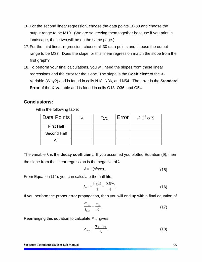
Spectrum Techniques Student Lab Manual
95
16. For the second linear regression, choose the data points 16-30 and choose the
output range to be M19. (We are squeezing them together because if you print in
landscape, these two will be on the same page.)
17. For the third linear regression, choose all 30 data points and choose the output
range to be M37. Does the slope for this linear regression match the slope from the
first graph?
18. To perform your final calculations, you will need the slopes from these linear
regressions and the error for the slope. The slope is the Coefficient of the X-
Variable (Why?) and is found in cells N18, N36, and N54. The error is the Standard
Error of the X-Variable and is found in cells O18, O36, and O54.
Conclusions:
Fill in the following table:
Data Points t1/2 Error # of ’s
First Half
Second Half
All
The variable is the decay coefficient. If you assumed you plotted Equation (9), then
the slope from the linear regression is the negative of
)(slope . (15)
From Equation (14), you can calculate the half-life:
693.0)2ln(
2/1 t . (16)
If you perform the proper error propagation, then you will end up with a final equation of
2/1
2/1
tt
. (17)
Rearranging this equation to calculate 2/1t gives
2/12/1
tt
. (18)

Spectrum Techniques Student Lab Manual
96
Now, to find the number of ’s that your result is away from the true value of t1/2 = 153 s,
we use the following equation
2/1
'#t
truemeasuredsof
. (19)
What you measure is the distance from your result to the true value and then see how
many standard deviations that is. The rule of thumb is that the result should be no
more than 2 ’s away from the true value to be statistically good.
Post-Lab Questions:
1. Write your result with the error, i.e. 153 s ± 1 s. Is this result (statistically)
good? (Recall that any value judgments must be justified.)
2. Which of the three results is better? Why?
3. How can the situation in #2 be resolved so that a linear regression over all the
data gives a more valid result? (How can you combine the halves of the
data?)

Spectrum Techniques Student Lab Manual
97
Data Sheet for Half-Life Lab
Tube #: Run Duration:
Dead Time: (Time)
Counts Corr. Counts ln(Counts) Time
(Background Count)
30
60
90
120
150
180
210
240
270
300
330
360
390
420
450
Name: Lab Session: Date: Partner:

Spectrum Techniques Student Lab Manual
98
Data Sheet for Half-Life Lab (Cont’d) Counts Corr. Counts ln(Counts) Time
480
510
540
570
600
630
660
690
720
Data t1/2 Error # of 's
First Half
Second Half
Whole
Don’t forget to hand in a graph of the data with this table.

Spectrum Techniques Student Lab Manual
99
Appendix A – SI Units The standard units of measure used in physics are the MKS (Meter, Kilogram, Second) version of the International System (SI) of Units. They are commonly referred to as the metric units. The latest version of the standards can be found in the following three resources: “Preferred Metric Units for General Use by the Federal Government,” (Federal
Standard 376B), January 27, 1993, General Services Administration. “Guide for the Use of International System of Units (SI),” (NIST Special Publication
811) (obtainable at the NIST website - http://www.nist.gov) “The International System of Units (SI),” (NIST Special Publication 330) (obtainable
at the NIST website – http://www.nist.gov)
Below, you will find the proper SI units – base and derived – that we will use. Also, there is a table showing the latest prefixes for SI Units.
Physical Quantity Name of Unit Symbol
Base Units
Length meter m Mass kilogram kg Time second t
Electric current ampere A Derived Units
Force newton N Energy joule J
electric potential volt V
electric resistance ohm electric capacitance farad F
activity (radioactive source) becquerel Bq
Table 1: Proper SI units that may be used in the lab manual.

Spectrum Techniques Student Lab Manual
100
Mulitplication Factor Prefix Name Prefix Symbol 1 000 000 000 000 000 000 000 000 = 1024 yotta Y 1 000 000 000 000 000 000 000 = 1021 zetta Z 1 000 000 000 000 000 000 = 1018 exa E 1 000 000 000 000 000 = 1015 peta P 1 000 000 000 000 = 1012 tera T 1 000 000 000 = 109 giga G 1 000 000 = 106 mega M 1 000 = 103 kilo k 100 = 102 hecto h 10 = 101 deca da 0.1 = 10-1 deci d 0.01 = 10-2 centi c 0.001 = 10-3 milli m 0.000 001 = 10-6 micro 0.000 000 001 = 10-9 nano n 0.000 000 000 001 = 10-12 pico p
0.000 000 000 000 001 = 10-15 femto f 0.000 000 000 000 000 001 = 10-18 atto a
0.000 000 000 000 000 000 001 = 10-21 zepto z 0.000 000 000 000 000 000 000 001 = 10-24 yocto y

Spectrum Techniques Student Lab Manual
101
Appendix B – Common Radioactive Sources Below is a list of commonly used radioactive sources. All of these sources are available from Spectrum Techniques, Inc. The standard radioisotopes sold by Spectrum Techniques, Inc. are exempt from NRC licensing and require no special handling, storage or disposal.
Isotope Generator
The Cs-137/Ba-137m Isotope Generator provides a convenient means of producing a short half-life isotope for demonstrating radioactive decay experiments. This improved design is based on the original Union Carbide patent and can produce up to 1000 samples of the Ba-137 isotope with a half-life of 2.6 minutes using a simple eluting solution of 0.9% NaCl. The kit is supplied complete with the Cs-137/Ba-137m generator, 250 ml of eluting solution, a syringe for the elution, planchets and a storage case.

Spectrum Techniques Student Lab Manual
102
Appendix C – Statistics
Statistics play a very important part of physics, especially nuclear physics,
because we are dealing with atoms that number on the order of Avogadro’s number. It
is impossible to deal with every single atom individually, so we rely on statistics to give
us a prediction of behavior.
Statistics uses two main quantities in predicting behavior, the mean and the
standard deviation. The mean is the average, what most of the particles are doing.
The standard deviation tells us how many particles are also doing almost the same
thing as the mean. The previous experience that students usually have with mean and
standard deviation is from mathematics class (unless a statistics class has been taken).
From this experience, they know that mean can formulated by
N
i
i
N
xx
0, (1)
where x is the mean of a set of measurements ix (i = 1, 2, 3, …, N), and N is the
number of measurements taken.
Most students can recall how to calculate the standard deviation
1
0
2
N
xxN
ii
. (2)
What this equation does is measure the variance without regard to direction above or
below the mean (that is why you square and then square root – it is equivalent to
absolute value which just measures distance). These equations hold for most
everything the students have dealt with up to this point in school. The reason is that
most measurements follow a Gaussian distribution (symmetric about a mean).
Counting in nuclear physics is not symmetric about a mean. There is usually
some count rate that is pretty small because probability of decay is pretty small. Then
you also get high count rates. (Look back at the data from the statistics experiments
you performed this year.) When the data collects to a small number with a bit of a tail,
this is no longer a Gaussian distribution. The standard three statistical distributions will

Spectrum Techniques Student Lab Manual
103
be discussed below to assist the student learning more in detail about the statistics of
counting in nuclear physics. There are many more statistical distributions used for
various reasons but they will not be discussed here. (An example is the Landau
distribution used in describing the energy loss of a charged particle in matter, which is
different because it has an infinitely long tail to it.)
The first distribution is the Binomial distribution. This distribution is used when
you have two possible outcomes, the probability of getting one of those outcomes (and
thus the other) is a constant number independent of the number of trials, and the
selection of either outcome does not affect that outcome again in later trials. A good
example of this is flipping a coin.
To look at an example, we have an experiment where there are only two
outcomes A and B. In a binomial distribution, we deal with p, the probability that you will
get one of the outcomes (A), and q, the probability that the other outcome occurs (B).
Sometimes, instead of q, statistics books use 1-p, which is how q is calculated. Then,
the binomial distribution gives the probability, P(n), that n out of N objects are A is given
by
nNnnNn ppnnN
Nqp
nnN
NnP
1
!!
!
!!
!)( . (3)
Now for this distribution the mean, m, is given by
pNm (4)
and the standard deviation is calculated with any of the following
)1( pNpNpqmq . (5)
In order to study radioactive decays, we need a more useful distribution. We
need one for a very large number of counts and one that can handle a very small
probability of success (large N and small p). It just happens that the Poisson
distribution is the special case of the binomial distribution given those two conditions.
The Poisson distribution gives the probability, P(n), that n out of N objects are A as
mn
en
mnP
!)( , (6)
where m is the mean of the distribution (m = Np). The nicest feature of the Poisson
distribution is the ease to calculate standard deviation. The formula is

Spectrum Techniques Student Lab Manual
104
m . (7)
But for individual measurements, we take the standard deviation to be the square root
of the number of counts, here N,
N . (8)
So if you have a count rate of 10,000 cpm, then the standard deviation is ±100 cpm.
You may have noticed that for large values of m, the Poisson distribution
becomes hard to use. So we use a special case of the Poisson distribution for m>20
(the accepted rule of thumb), or a different special case of the Binomial distribution that
has large counts, low probability, and a large mean. This new distribution is called the
Normal or Gaussian distribution. This is the distribution that most students are familiar
with, its common name is the bell curve. Another added feature of this distribution is
that it can handle continuous variables (like most of those in our experiments), unlike
the Poisson and Binomial distributions, which can only handle discrete variables*. The
Gaussian distribution is given by
2
2
2exp
2
1)(
mx
nP . (9)
This equation gives us the mean and standard deviation equations that we are
accustomed to in Equations (1) and (2).
More details about statistical distributions must be researched in other books.
There is a huge amount of resources out there, statistical books and methods in
experimental physics books abound. There are some of the latter books listed below if
you wish to do more research. These should be available at most university libraries, or
through interlibrary loan services.
1. P.R. Bevington, D.K. Robinson, Data Reduction and Error Analysis for the Physical
Sciences, (McGraw-Hill, 1992).
2. G. Knoll, Radiation Detection and Measurement, (John Wiley & Sons, 1989)**.
3. N. Tsoulfanidis, Measurement and Detection of Radiation, (McGraw-Hill, 1995).
* The number of counts is a discrete, there is no such thing as a fraction of a count (there is nothing between 1 and 2). Length is a continuous variable, between 1 and 2 is 1.5. Between 1 and 1.5 is 1.25 and so on. * * There is a newer edition this one. This edition is the one the author owns.

Spectrum Techniques Student Lab Manual
105
4. W.R. Leo, Techniques for Nuclear and Particle Physics Experiments, (Springer-
Verlag, 1994)
Linear Regression
When Excel® or a graphing calculator performs a linear regression, it makes two
calculations to determine the slope and y-intercept of the best-fit line for the data. How
does it do it? Linear regressions are carried out using the method of least squares. This
method finds the line that minimizing the distance all the data points are away from the
best-fit line. This may sound complicated but it is really not if you know a little algebra
and one concept from calculus. Recall, that in math to find distance we use absolute
value, which is equivalent to the square root of the square*. (The squaring and
subsequent square rooting of a quantity is a common mathematical trick to substitute
taking an absolute value.) Let us start with an experiment, where you measure
variables x and y over N trials. The expected result is
y = mx + b
but remember that we take N measurements. So we get
y1 = mx1 + b
y2 = mx2 + b
….
yN = mxN + b.
These equations are not in general consistent; if we take different pairs of
equations, and solve them for m and b, we obtain different values for m and b. The
reason for the various values of m and b, of course, is that there are experimental errors
in the yi. Since the two sides of the equation, yi = mxi + b, are not exactly equal, but
differ by an amount let’s call d. To calculate d, we use
di = mxi + b – yi,
where di is the deviation corresponding to the ith equation and the pair of observations
(xi, yi). Since the values for di are the results of the experimental errors, we can assume
* The terms for absolute value and square root of a square are equivalent. That is
2xx .

Spectrum Techniques Student Lab Manual
106
that they are distributed according to the Gaussian (or normal) distribution. This allows
us to use the method of maximum likelihood to find the most probable values of m and
b.
This method finds the most probable values of m and b by minimizing the sum of
the squares of the deviations. That is, we minimize the quantity, d2, which has the form
i
iii ybmxd 22
.
The principle of least squares is finding the values of m and b that minimize d2. To
minimize the two variables, we take the partial derivative (due to the fact that m and b
are in the equation) of the function with respect to each of the variables (m and b) in
turn and set each derivative equal to zero. Rearranging the equations, we get 1
bNxmy ii and iiii xbxmyx 2,
where N is the number of points that are being used in the fitting process. Further
rearrangement, gives the following results for m and b:
22ii
iiyi
xxN
yxyxNm and
22
2
ii
iiiii
xxN
xyxxyb .
These values for m and b, are the slope and y-intercept, respectively, for the best-fit line
for the data. This is the calculation that a computer or calculator makes to output the
equation of the best-fit line.
Propagation of Errors
Often in laboratory experiments, the results will not be measured directly.
Rather, the results will be calculated from several measured physical quantities. Each
of these measured quantities consists of a mean (average) value and an error. What is
the resulting error in the final result of such an experiment? It is difficult to say how the
error of the measured quantities will translate (or propagate) to the error of the final
result.
The difficulty arises because we do not which sign, plus or minus, really exists for
the error. Recall that when reporting error, we show both signs, ±, to indicate that we
1 The summations, , are still over the index i but it has been dropped for convenience.

Spectrum Techniques Student Lab Manual
107
do not truly know where the true values lie. As an example, assume that we measure
two quantities, A ± A and B±B. (A and B represent the error on A and B,
respectively.) Then, we combine A and B into Z by Z = A + B. The extreme values of
the error are easy to predict, they are given by
BABABBAA or BABABBAA .
The problem is that most likely there is a mixture, some error from A cancels some of
the error or vice-versa. Then the situation becomes more complicated. However, this
problem has arisen before, the distance between two points on the Cartesian plane.
There we treat the distances independently (actually, perpendicular), but combine them
by the Pythagorean theorem. Simple enough solution, but what if the result, Z, depends
on both A and B (Z is a function of A and B). Then the problem uses the same method
but involves partial derivatives. (Note: The author considers this too complex of a
concept to explain here and refers any interested readers to their instruction or
multivariable calculus textbooks.) Due to the complexity of the work with partial
derivatives, the results of the error for various operations are given in the table below.
Operation Relation between Z, A, and B
Z = A + B 222 BAZ
Z = A – B 222 BAZ
Z = AB 222
B
B
A
A
Z
Z
Z = A/B 222
B
B
A
A
Z
Z
Z = nA *
A
An
Z
Z
Z = ln (A)
A
AZ
Z = eA
AZ
Z
* n is a constant (any real number)

Spectrum Techniques Student Lab Manual
108
Any further discussion of data analysis and error analysis techniques should be referred
to Taylor, John R. An Introduction to Error Analysis: The Study of Uncertainties in
Physical Measurements. University Science Books, 1982.

Spectrum Techniques Student Lab Manual
109
Appendix D - Radiation Passing Through Matter Our three forms of radiation must interact with matter while passing through it or
we would never be able to detect them. However, how they interact with matter is
completely different. Therefore, I will break this appendix up into three sections to study
alpha particles, beta particles, and gamma rays individually.
Alpha Particles
Alpha particles are helium nuclei, two protons and two neutrons, so it is
considered a heavy particle (compared to other particles in the universe). As an alpha
particle passes through matter, it passes close to many atoms. The positive charge
from the alpha particle attracts an electron from the valence shell of an atom it passes.
Sometimes the attraction is strong enough to free the electron from the atom, this
process is known as ionization. During this process, the alpha particle ends up giving
up some energy to the freed electron. This is the only true interaction that the alpha has
besides depositing its energy in some atoms through inelastic collisions. Either way,
the alpha particle loses some energy each time it interacts, which is denoted by
physicists as dE/dx. To calculate dE/dx, one uses the Bethe-Bloch formula which is
Z
C22
2ln
A
Z2 2
2max
22
2
222
I
WvmzcmrN
dx
dE eeea (1)
where 2 0 15352 2 2N r m c M eV cm ga e e . / and
re: classical electron radius = 2.817 x 10⁻¹³ cm me: electron mass = 9.11 x 10⁻³¹ kg
Na: Avogrado’s number = 6.022 x 10²³ / mol I: mean ionization energy
Z: atomic number of absorbing material A: atomic mass of absorbing material
: density of absorbing material z: charge of incident particle in units of e
= v/c of the incident particle = 1
1 2
: density correction C: shell correction
Wmax: maximum energy transfer in a single collision 22 cme .

Spectrum Techniques Student Lab Manual
110
Note that the equation for dE/dx is negative to indicate that it is an energy loss. There
are two correction terms, one for density effects and one for shell effects. While there
are many other possible corrections that could be made, they are negligible ( 1%).
The density effect arises due to the fact that atoms in the matter are polarized
by the electric field of the alpha particle passing through it. Thus, the electrons on the
far side of the atom will be shielded from interactions with the particle. However, the
denser the material, the closer the atoms are together and more shielding that occurs.
Since this term takes away possible interactions, is subtracted from the original formula.
The shell effect gives a small correction to the Bethe-Bloch formula, but still
must be taken into account. This effect only occurs when the velocity of the incident
particle is equal to or less than the orbital speed of the electrons. This situation
invalidates the assumption that the electrons are stationary with respect to the incident
particle.
While an alpha particle will lose energy in a collision, it is not much to make it
stray from its path. Therefore, an alpha particle passing through matter traverses it in a
relatively straight path while giving up energy in mainly ionization interactions.
Beta Particles
Beta particles are electrons that are emitted by the nucleus. They also undergo
the ionization energy loss as predicted by the Bethe-Bloch formula (Equation 1).
However, electrons are much less massive than alpha particles, m m 7342 , so there
is additional interaction due to the fact that the beta particle is greatly scattered through
matter. A beta particle passing close to a nucleus can have an electromagnetic
interaction that will slow the beta down and cause it to change directions; in essence it
will be braking. This “braking radiation” is described by its German name,
bremmstrahlung. Whenever the beta particle undergoes bremmstrahlung, it loses
energy but when an electron changes energy, it must absorb or emit electrons. Thus,
bremmstrahlung is the production of x-ray photons due to the interactions of electrons
(beta particles) with nuclei in matter.

Spectrum Techniques Student Lab Manual
111
Again, an alpha particle will pass almost straight through matter. The opposite is
true for a beta particle. It undergoes multiple scatterings that cause it path to be very
much of a “zigzag” pattern with no way to predict its path.
Gamma Rays
Gamma rays are photons that have an energy, frequency, and wavelength
sufficient enough to be classified as a gamma ray in the electromagnetic spectrum.
Photons interact three different ways in matter: (1) Photoelectric effect, (2) Compton
scattering, and (3) Pair production.
The photoelectric effect is when a photon is absorbed by an electron with the
subsequent ejection of the electron from the atom. The maximum energy of the ejected
electron is given by
KE Emax (2)
where E is the energy of the incident photon and is the work function (energy
necessary to free the electron).
Compton scattering is the scattering of photons on electrons. Originally, this
was only for free electrons but if the photon energy is sufficient to overcome the binding
energy, then we can consider the electron as free. In this collision, the photon is
incident on the electron with an energy h, where h is Planck’s constant and n is the
frequency of the photon. The photon undergoes an inelastic collision with the electron,
so the photon gives some of its energy to the electron. The photon leaves with a new
energy h’ and the electron leaves with a certain amount of kinetic energy that is E =
h-h’. We can calculate h’ by determining the scattering angle of the photon, . Then
we can use the equation:
cos11
hh (3)
The process of pair production refers to the transformation of a photon into an
electron-positron pair. In order to conserve momentum, this process can only occur
when the photon is close to the nucleus. Theoretically, the photon needs only the
energy that equates to the mass of an electron-positron pair. This energy is 1.022 MeV.
However, this process very, very rarely occurs below 1.5 MeV of photon energy,

Spectrum Techniques Student Lab Manual
112
because nature does not like creating the electron and positron and then having them
just sit there. Therefore, pair production only occurs when there is not only the mass
(energy) available, but also some extra energy for kinetic energy for the electron and
positron.
The photoelectric effect dominates for photon energies from 4 eV up to 0.5
MeV. Then Compton scattering dominates up to 2 MeV. Finally, pair production
dominates above 10 MeV, but only if a nucleus is present to absorb the momentum.
(Between 2 MeV and 10 MeV there is no true dominating absorption mechanism for
photons.)
For further reading on this topic, please refer to the Suggested References
section.

Spectrum Techniques Student Lab Manual
113
Appendix E – Suggested References
There is a large amount of information in books, journal articles, and on the Internet
relating to the topics in this lab manual (Radiation, particle interaction with matter, and
particle detection). Since many high school teachers do not have access to journals, I
have only listed books and website references.
Two of the best books on the topics of particle detectors that cover Geiger counters
are
Knoll, G. Radiation Detection and Measurement, John Wiley & Sons, 1989.
Tsoulfanidis, N. Measurement and Detection of Radiation, McGraw-Hill, 1995.
As for websites, there is a very large number of websites that would consume page
after page of this manual. Instead, this is a small sample of websites, which represent
the ones that the author deemed most helpful while writing this manual. They are not
listed in any particular order of importance, just alphabetically. Also, these sites were
verified in July of 2002, and any further accuracy of the information cannot be
guaranteed. In addition, if further resources are desired, do a search on a website such
as Google (http://www.google.com).
American Nuclear Society – http://www.ans.org This is the professional organization for nuclear engineers, nuclear scientists, and other nuclear related professionals. They sponsor very good programs for teachers in different areas of the country. There is large public information section covering many different levels of education.
EPA – Radiation Protection Program – http://www.epa.gov/radiation
This is the EPA’s webpage for how to protect the environment from radiation’s harm and explains how they clean it up after it happens. The EPA also tries to educate people that not all radiation is harmful.

Spectrum Techniques Student Lab Manual
114
Health Physics Society – http://www.hps.org
This is the professional organization for health physicists. It has more public information available, as well as an “Ask the Expert” area. Some of its regional chapters are excellent resources as well.
Nuclear Engineering 104A: Radiation Detection and Nuclear
Instrumentation Laboratory (Fall 2001) – http://www.nuc.berkeley.edu/dept/Courses/NE_104A
This link leads you to a list of files that comprise the course information. There is no main page that accesses all of the files. This course contains many materials on the basics of radiation and its detection.
RadEFX Radiation Health Effects Information Resource - http://radefx.bcm.tmc.edu/chernobyl
This is a very neat webpage where experts answer questions from basic radiation facts to questions mainly focusing on the worldwide effects of Chernobyl.
Radiological Information from the Collider-Acceleration Group at Brookhaven National Laboratory – http://www.agsrhichome.bnl.gov/AGS/Accel/SND/radiological_information.htm
This site covers radiation safety information from the most basic form to the very advanced concepts that are involved at the AGS and RHIC particle colliders at BNL. The link on elements is very good.
Texas Department of Health – Bureau of Radiation Control –
http://www.tdh.state.tx.us/ech/rad/pages/brc.htm
This is the website of the State’s controlling entity in Texas. (It is suggested that you find your state’s radiation department for information relevant to your state.) There may or may not be education information available, it depends on the state.
Spectrum Techniques Student Lab Manual
115
The Radiation and Health Physics Page – http://www.umich.edu/~radinfo/nojava.html
This is perhaps one of the best, or at least most referenced, webpage dealing with radiation on the Internet. It is a comprehensive website that does supply educational resources.
US Nuclear Regulatory Commission – http://www.nrc.gov
Find out what the controlling entity in the US for radiation does. There are also public information materials available.
University of Waterloo Radiation Safety Training – http://www.rstp.uwaterloo.ca
Good online training manual with a lot of basic information using animated gifs. Many of the particle interactions with matter are animated.
Uranium Information Centre (Melbourne, Australia) – http://www.uic.com.au/ral.htm
This is an awesome introduction to radiation all around us in everyday life. There are many good cartoon figures that explain the concepts being discussed.
Worcester Polytechnic Institute’s Radiation Safety Training and Reference Manual – http://www.wpi.edu/Admin/Safety/RSO/Training/trm.html
This radiation safety manual is online and covers the basics for many different professions that interact with radiation.

Spectrum Techniques Student Lab Manual
116
Appendix F – NRC Regulations
10 CFR 30.18, 30.71 Schedule B, and 32.19
§30.18 Exempt quantities. (a) Except as provided in paragraphs (c) and (d) of this section, any person is exempt from the requirements for a license set forth in section 81 of the Act and from the regulations in parts 30 through 34, 36 and 39 of this chapter to the extent that such person receives, possesses, uses, transfers, owns, or acquires byproduct material in individual quantities each of which does not exceed the applicable quantity set forth in §30.71, Schedule B. (b) Any person who possesses byproduct material received or acquired prior to September 25, 1971 under the general license then provided in §31.4 of this chapter is exempt from the requirements for a license set forth in section 81 of the Act and from the regulations in parts 30 through 34 of this chapter to the extent that such person possesses, uses, transfers, or owns such byproduct material. (c) This section does not authorize for purposes of commercial distribution the production, packaging, repackaging, or transfer of byproduct material or the incorporation of byproduct material into products intended for commercial distribution. (d) No person may, for purposes of commercial distribution, transfer byproduct material in the individual quantities set forth in §30.71 Schedule B, knowing or having reason to believe that such quantities of byproduct material will be transferred to persons exempt under this section or equivalent regulations of an Agreement State, except in accordance with a license issued under §32.18 of this chapter, which license states that the byproduct material may be transferred by the licensee to persons exempt under this section or the equivalent regulations of an Agreement State. [35 FR 6427, Apr. 22, 1970, as amended at 36 FR 16898, Aug. 26, 1971; 43 FR 6921, Feb. 17, 1978; 52 FR 8241, Mar. 17, 1987; 58 FR 7736, Feb. 9, 1993] §30.71 Schedule B.

Spectrum Techniques Student Lab Manual
117
Byproduct material Microcuries
Antimony 122 (Sb 122) 100 Antimony 124 (Sb 124) 10 Antimony 125 (Sb 125) 10
Arsenic 73 (As 73) 100 Arsenic 74 (As 74) 10 Arsenic 76 (As 76) 10 Arsenic 77 (as 77) 100
Barium 131 (Ba 131) 10 Barium 133 (Ba 133) 10 Barium 140 (Ba 140) 10 Bismuth 210 (Bi 210) 1 Bromine 82 (Br 82) 10
Cadmium 109 (Cd 109) 10 Cadmium 115m (Cd 115m) 10
Cadmium 115 (Cd 115) 100 Calcium 45 (Ca 45) 10 Calcium 47 (Ca 47) 10
Carbon 14 © 14) 100 Cerium 141 (Ce 141) 100 Cerium 143 (Ce 143) 100 Cerium 144 (Ce 144) 1 Cesium 131 (Cs 131) 1,000
Cesium 134m (Cs 134m) 100 Cesium 134 (Cs 134) 1 Cesium 135 (Cs 135) 10 Cesium 136 (Cs 136) 10 Cesium 137 (Cs 137) 10 Chlorine 36 (Cl 36) 10 Chlorine 38 (Cl 38) 10
Chromium 51 (Cr 51) 1,000 Cobalt 58m (Co 58m) 10
Cobalt 58 (Co 58) 10 Cobalt 60 (Co 60) 1 Cobalt 64 (Cu 64) 100
Dysprosium 165 (Dy 165) 10 Dysprosium 166 (Dy 166) 100
Erbium 169 (Er 169) 100 Erbium 171 (Er 171) 100
Europium 152 9.2 h (Eu 152 9.2 h)
100
Europium 152 13 yr (Eu 152 13 yr)
1
Europium 154 (Eu 154) 1 Europium 155 (Eu 155) 10
Fluorine 18 (F 18) 1,000 Gadolinium 153 (Gd 153) 10 Gadolinium 159 (Gd 159) 100
Gallium 72 (Ga 72) 10 Germanium 71 (Ga 71) 100
Gold 198 (Au 198) 100 Gold 199 (Au 199) 100
Hafnium 181 (Hf 181) 10 Holmium 166 (Ho 166) 100
Hydrogen 3 (H3) 1,000 Indium 113m (In 113m) 100 Indium 114m (In 114m) 10 Indium 115m (In 115m) 100
Indium 115 (In 115) 10 Iodine 125 (I 125) 1 Iodine 126 (I 126) 1 Iodine 129 (I 129) 0,1 Iodine 131 (I 131) 1 Iodine 132 (I 132) 10 Iodine 133 (I 133) 1 Iodine 134 (I 134) 10 Iodine 135 (I 135) 10
Iridium 192 (Ir 192) 10 Iridium 194 (Ir 194) 100
Iron 55 (Fe 55) 100 Iron 59 (Fe 59) 10
Krypton 85 (Kr 85) 100 Krypton 87 (Kr 87) 10
Lanthanum 140 (La 140) 10 Lutetium 177 (Lu 177) 100 Manganese 52 (Mn 52) 10 Manganese 54 (Mn 54) 10 Manganese 56 (Mn 56) 10
Mercury 197m (Hg 197m) 100 Mercury 197 (Hg 197) 100 Mercury 203 (Hg 203) 10
Molbdenum 99 (Mo 99) 100 Neodymium 147 (Nd 147) 100 Neodymium 149 (Nd 149) 100
Nickel 59 (Ni 59) 100 Nickel 63 (Ni 63) 10 Nickel 65 (Ni 65) 100
Niobium 93m (Nb 93m) 10 Niobium 95 (Nb 95)` 10 Niobium 97 (Nb 97) 10

Spectrum Techniques Student Lab Manual
118
Osmium 185 (Os 185) 10 Osmium 191m (Os 191) 100 Osmium 191 (Os 191) 100 Osmium 193 (Os 193) 100
Palladium 103 (Pd 103) 100 Palladium 109 (Pd 109) 100 Phosphorus 32 (P 32) 10 Platinum 191 (Pt 191) 100
Platinum 193m (Pt 193m) 100 Platinum 193 (Pt 193) 100
Platinum 197m (Pt 197m) 100 Platinum 197 (Pt 197) 100 Polonium 210 (Po 210) 0.1
Potassium 42 (K 42) 10 Praseodymium 142 (Pr 142) 100 Praseodymium 143 (Pr 143) 100 Promethium 147 (Pm 147) 10 Promethium 149 (Pm 149) 10
Rhenium 186 (Re 186) 100 Rhenium 188 (Re 188) 100
Rhodium 103m (Rh 103m) 100 Rhodium 105 (Rh 105) 100
Rubidium 86 (R86) 10 Rubidium 87 (Rb87) 10
Ruthenium 97 (Ru 97) 100 Ruthenium 103 (Ru 103) 10 Ruthenium 105 (Ru 105) 10 Ruthenium 106 (Ru 106) 1 Samarium 151 (Sm 151) 10 Samarium 153 (Sm 153) 100
Scandium 46 (Sc 46) 10 Scandium 47 (Sc 47) 100 Scandium 48 (Sc 48) 10 Selenium 75 (Se 75) 10
Silicon 31 (Si 31) 100 Silver 105 (Ag 105) 10
Silver 110m (Ag 110m) 1 Silver 111 (Ag 111) 100 Soldium 24 (Na 24) 10 Strontium 85 (Sr 85) 10 Strontium 89 (Sr 89) 1 Strontium 90 (Sr 90) 0.1 Strontium 91 (Sr 91) 10 Strontium 92 (Sr 92) 10
Sulphur 35 (S 35) 100 Tantalum 182 (Ta 182) 10 Technetium 96 (Tc 96) 10
Technetium 97m (Tc 97m) 100 Technetium 97 (Tc 97) 100
Technetium 99m (Tc 99m) 100 Technetium 99 (Tc 99) 10
Tellurium 125 m (Te 125 m) 10 Tellurium 127m (Te 127m) 10
Tellurium 127 (Te 127) 100 Tellurium 129m (Te 129m) 10
Tellurium 129 (Te 129) 100 Tellurium 131m (Te 131m) 10
Tellurium 132 (Te 132) 10 Terbium 160 (Tb 160) 10 Thallium 200 (Tl 200) 100 Thallium 201 (Tl 201) 100 Thallium 202 (Tl 202) 100 Thallium 204 (Tl 204) 10 Thulium 170 (Tm 170) 10 Thulium 171 (Tm 171) 10
Tin 113 (Sn 113) 10 Tin 125 (Sn 125) 10
Tungsten 181 (W 181) 10 Tungsten 185 (W 185) 10 Tungsten 187 (W 187) 100 Vanadium 48 (V 48) 10
Xenon 131m (Xe 131m) 1,000 Xenon 133 (Xe 133) 100 Xenon 135 (Xe 135) 100
Ytterbium 175 (Yb 175) 100 Yttrium 90 (Y 90) 10 Yttrium 91 (Y91) 10 Yttrium 92 (Y92) 100 Yttrium 93 (Y93) 100 Zinc 65 (Zn 65) 10
Zinc 69m (Zn 69m) 100 Zinc 69 (Zn 69) 1,000
Zirconium 93 (Zr 93) 10 Zirconium 95 (Zr 95) 10 Zirconium 97 (Zr 97) 10
Any byproduct material not listed above other than alpha emitting byproduct materials
0.1

Spectrum Techniques Student Lab Manual
119
§32.19 Same: Conditions of licenses. Each license issued under §32.18 is subject to the following conditions: (a) No more than 10 exempt quantities set forth in §30.71, Schedule B of this chapter shall be sold or transferred in any single transaction. For purposes of this requirement, an individual exempt quantity may be composed of fractional parts of one or more of the exempt quantities in §30.71, Schedule B of this chapter, provided that the sum of such fractions shall not exceed unity. (b) Each quantity of byproduct material set forth in §30.71, Schedule B of this chapter shall be separately and individually packaged. No more than 10 such packaged exempt quantities shall be contained in any outer package for transfer to persons exempt pursuant to §30.18 of this chapter. The outer package shall be such that the dose rate at the external surface of the package does not exceed 0.5 millirems per hour. (c) The immediate container of each quantity or separately packaged fractional quantity of byproduct material shall bear a durable, legible label which (1) identifies the radioisotope and the quantity of radioactivity, and (2) bears the words "Radioactive Material." (d) In addition to the labeling information required by paragraph (c) of this section, the label affixed to the immediate container, or an accompanying brochure, shall also (1) state that the contents are exempt from NRC or Agreement State licensing requirements; (2) bear the words "Radioactive Material -- Not for Human Use -- Introduction Into Foods, Beverages, Cosmetics, Drugs, or Medicinals, or Into Products Manufactured for Commercial Distribution is Prohibited -- Exempt Quantities Should Not be Combined"; and (3) set forth appropriate additional radiation safety precautions and instructions relating to the handling, use, storage, and disposal of the radioactive material. [35 FR 6428, Apr. 22, 1970]
Contact us: If we may be of help to you, feel free to contact us. Visit our web site for up-to-date information and products.
Spectrum Techniques, LLC
106 Union Valley Road
Oak Ridge, TN 37830 USA
Phone: 865-482-9937 FAX 865-483-0473
Email: [email protected]
Web site: www.SpectrumTechniques.com

Spectrum Techniques
Lab Manual Student Version
Revised, March 2014

Spectrum Techniques Student Lab Manual
2
Table of Contents Student Usage of this Lab Manual ................................................. 3 What is Radiation? ......................................................................... 4 Introduction to Geiger-Müller Counters .......................................... 8 Good Graphing Techniques ......................................................... 10
Experiments
1. Plotting a Geiger Plateau .............................................. 12 2. Statistics of Counting ................................................... 20 3. Background ................................................................... 26 4. Resolving Time ............................................................. 30 5. Geiger Tube Efficiency .................................................. 37 6. Shelf Ratios ................................................................... 43 7. Backscattering............................................................... 48 8. Inverse Square Law ...................................................... 57 9. Range of Alpha Particles ............................................... 62 10. Absorption of Beta Particles .......................................... 69 11. Beta Decay Energy ....................................................... 74 12. Absorption of Gamma Rays .......................................... 80 13. Half-Life of Ba-137m ..................................................... 88
Appendices
A. SI Units ......................................................................... 99 B. Common Radioactive Sources .................................... 101 C. Statistics ...................................................................... 102 D. Radiation Passing Through Matter .............................. 109 E. Suggested References ................................................ 113 F. NRC Regulations ........................................................ 116

Spectrum Techniques Student Lab Manual
3
Student Usage of Lab Manual This manual is written to help students learn as much as possible about radiation
and some of the concepts key to nuclear and particle physics. This manual in particular
is written to guide you through a laboratory experiment set-up. The lab manual has the
following layout:
Detailed background material on radiation, the Geiger-Müller counter and its
operation, and radiation interaction with matter.
Thirteen laboratory experiments with instructions, data sheets, and analysis
instruction.
A piece of standalone equipment from Spectrum Techniques may not be entirely
equipped for the laboratory environment. Additional resources and recommendations
are made in the teacher’s notes of the experimental write-ups for schools that wish to
run the specific experiments. Also, schools operate on different class schedules,
varying from 42-minute periods to 3-hour lab sessions. Thus, the labs are written with
flexibility to combine them in different manners (our suggestions are listed below).
The lab manual is not intended to be a “recipe” book but a guide on how to obtain
the data and analyze it to answer certain questions. What this means is that explicit
directions as to every single button to push are not given, but the student will have
guidance where this can be inferred.
NOTE: All directions in this laboratory manual assume the use of a PC computer
with Microsoft Excel® used for the experiments. Any manual operation has the
appropriate directions given in the product manual. All operations listed in the directions
below may be carried out on the screen of the Spectrum Techniques equipment. Also,
all instructions use the ST-360 model Geiger-Müller counter, but the other models, ST-
160 and ST-260, have similar functions available.

Spectrum Techniques Student Lab Manual
4
What is Radiation?
This section will give you some of the basic information from a quick guide of the
history of radiation to some basic information to ease your mind about working with
radioactive sources. More information is contained in the introduction parts of the
laboratory experiments in this manual.
Historical Background
Radiation was discovered in the late 1800s. Wilhelm Röntgen observed
undeveloped photographic plates became exposed while he worked with high voltage
arcs in gas tubes, similar to a fluorescent light. Unable to identify the energy, he called
them “X” rays. The following year, 1896, Henri Becquerel observed that while working
with uranium salts and photographic plates, the uranium seemed to emit a penetrating
radiation similar to Röntgen’s X-rays. Madam Curie called this phenomenon
“radioactivity”. Further investigations by her and others showed that this property of
emitting radiation is specific to a given element or isotope of an element. It was also
found that atoms producing these radiations are unstable and emit radiation at
characteristic rates to form new atoms.
Atoms are the smallest unit of matter that retains the properties of an element
(such as hydrogen, carbon, or lead). The central core of the atom, called the nucleus, is
made up of protons (positive charge) and neutrons (no charge). The third part of the
atom is the electron (negative charge), which orbits the nucleus. In general, each atom
has an equal amount of protons and electrons so that the atom is electrically neutral.
The atom is made of mostly empty space. The atom’s size is on the order of an
angstrom (1 Å), which is equivalent to 1x10⁻¹⁰ m while the nucleus has a diameter of a
few fermis, or femtometers, which is equivalent to 1x10-15 m. This means that the
nucleus only occupies approximately 1/10,000 of the atom’s size. Yet, the nucleus
controls the atom’s behavior with respect to radiation. (The electrons control the
chemical behavior of the atom.)

Spectrum Techniques Student Lab Manual
5
Radioactivity
Radioactivity is a property of certain atoms to spontaneously emit particles or
electromagnetic wave energy. The nuclei of some atoms are unstable, and eventually
adjust to a more stable form by emission of radiation. These unstable atoms are called
radioactive atoms or isotopes. Radiation is energy emitted from radioactive atoms,
either as electromagnetic (EM) waves or as particles. When radioactive (or unstable)
atoms adjust, it is called radioactive decay or disintegration. A material containing a
large number of radioactive atoms is called either a radioactive material or a radioactive
source. Radioactivity, or the activity of a radioactive source, is measured in units
equivalent to the number of disintegrations per second (dps) or disintegrations per
minute (dpm). One unit of measure commonly used to denote the activity of a
radioactive source is the Curie (Ci) where one Curie equals thirty seven billion
disintegrations per second.
1 Ci = 3.7x10¹⁰ dps = 2.2x10¹² dpm
The SI unit for activity is called the Becquerel (Bq) and one Becquerel is equal to one
disintegration per second.
1 Bq = 1 dps = 60 dpm
Origins of Radiation
Radioactive materials that we find as naturally occurring were created by:
1. Formation of the universe, producing some very long lived radioactive elements,
such as uranium and thorium.
2. The decay of some of these long-lived materials into other radioactive materials like
radium and radon.
3. Fission products and their progeny (decay products), such as xenon, krypton, and
iodine.
Man-made radioactive materials are most commonly made as fission products or
from the decays of previously radioactive materials. Another method to manufacture

Spectrum Techniques Student Lab Manual
6
radioactive materials is activation of non-radioactive materials when they are
bombarded with neutrons, protons, other high-energy particles, or high-energy
electromagnetic waves.
Exposure to Radiation
Everyone on the face of the Earth receives background radiation from natural
and man-made sources. The major natural sources include radon gas, cosmic
radiation, terrestrial sources, and internal sources. The major man-made sources are
medical/dental sources, consumer products, and other (nuclear bomb and disaster
sources).
Radon gas is produced from the decay of uranium in the soil. The gas migrates
up through the soil, attaches to dust particles, and is breathed into our lungs. The
average yearly dose in the United States is about 200 mrem/yr. Cosmic rays are
received from outer space and our sun. The amount of radiation depends on where you
live; lower elevations receive less (~25 mrem/yr) while higher elevations receive more
(~50 mrem/yr). The average yearly dose in the United States is about 28 mrem/yr.
Terrestrial sources are sources that have been present from the formation of the Earth,
like radium, uranium, and thorium. These sources are in the ground, rock, and building
materials all around us. The average yearly dose from these sources in the United
States is about 28 mrem/yr. The last naturally occurring background radiation source is
due to the various chemicals in our own bodies. Potassium (40K) is the major
contributor and the average yearly dose in the United States is about 40 mrem/yr.
Background radiation can also be received from man-made sources. The most
common is the radiation from medical and dental x-rays. There is also radiation used to
treat cancer patients. The average yearly dose in the United States is about 54
mrem/yr. There are small amounts of radiation in consumer products, such as smoke
detectors, some luminous dial watches, and ceramic dishes (with an orange glaze). The
average yearly dose in the United States is about 10 mrem/yr. The other man-made
sources are fallout from nuclear bomb testing and usage, and from accidents such as
Chernobyl. That average yearly dose in the United States is about 3 mrem/yr.

Spectrum Techniques Student Lab Manual
7
Adding up the naturally occurring and man-made sources, we receive on
average about 360 mrem/yr of radioactivity exposure. What significance does this
number have since millirems have not been discussed yet? Without overloading you
with too much information, the government states the safety level for radiation exposure
5,000 mrem/yr. (This is the Department of Energy’s Annual Limit.) This is three times
below the level of exposure for biological damage to occur. So just living another year
(celebrating your birthday), you receive about 7% of the government regulated radiation
exposure. If you have any more questions, please ask your teacher.
Spectrum Techniques Student Lab Manual
8
The Geiger-Müller Counter Geiger-Müller (GM) counters were invented by H. Geiger and E.W. Müller in
1928, and are used to detect radioactive particles ( and ) and rays ( and x). A GM
tube usually consists of an airtight metal cylinder closed at both ends and filled with a
gas that is easily ionized (usually neon, argon, and halogen). One end consists of a
“window” which is a thin material, mica, allowing the entrance of alpha particles. (These
particles can be shielded easily.) A wire, which runs lengthwise down the center of the
tube, is positively charged with a relatively high voltage and acts as an anode. The tube
acts as the cathode. The anode and cathode are connected to an electric circuit that
maintains the high voltage between them.
When radiation enters the GM tube, it will ionize some of the atoms of the gas*.
Due to the large electric field created between the anode and cathode, the resulting
positive ions and negative electrons accelerate toward the cathode and anode,
respectively. Electrons move or drift through the gas at a speed of about 104 m/s, which
is about 104 times faster than the positive ions move. The electrons are collected a few
microseconds after they are created, while the positive ions would take a few
milliseconds to travel to the cathode. As the electrons travel toward the anode they
ionize other atoms, which produces a cascade of electrons called gas multiplication or a
(Townsend) avalanche. The multiplication factor is typically 106 to 108. The resulting
discharge current causes the voltage between the anode and cathode to drop. The
counter (electric circuit) detects this voltage drop and recognizes it as a signal of a
particle’s presence. There are additional discharges triggered by UV photons liberated
in the ionization process that start avalanches away from the original ionization site.
These discharges are called Geiger-Müller discharges. These do not effect the
performance as they are short-lived.
Now, once you start an avalanche of electrons how do you stop or quench it?
The positive ions may still have enough energy to start a new cascade. One (early)
method was external quenching, which was done electronically by quickly ramping
down the voltage in the GM tube after a particle was detected. This means any more

Spectrum Techniques Student Lab Manual
9
electrons or positive ions created will not be accelerated towards the anode or cathode,
respectively. The electrons and ions would recombine and no more signals would be
produced.
The modern method is called internal quenching. A small concentration of a
polyatomic gas (organic or halogen) is added to the gas in the GM tube. The quenching
gas is selected to have a lower ionization potential (~10 eV) than the fill gas (26.4 eV).
When the positive ions collide with the quenching gas’s molecules, they are slowed or
absorbed by giving its energy to the quenching molecule. They break down the gas
molecules in the process (dissociation) instead of ionizing the molecule. Any quenching
molecule that may be accelerated to the cathode dissociates upon impact producing no
signal. If organic molecules are used, GM tubes must be replaced as they permanently
break down over time (after about one billion counts). However, the GM tubes included
in Spectrum Techniques® set-ups use a halogen molecule, which naturally recombines
after breaking apart.
For any more specific details, we will refer the reader to literature such as G.F.
Knoll’s Radiation Detection and Measurement (John Wiley & Sons) or to Appendix E of
this lab manual.
* A -ray interacts with the wall of the GM tube (by Compton scattering or photoelectric effect) to produce an electron that passes to the interior of the tube. This electron ionizes the gas in the GM tube.

Spectrum Techniques Student Lab Manual
10
Physics Lab
Good Graphing Techniques Very often, the data you take in the physics lab will require graphing. The following are a few general instructions that you will find useful in creating good, readable, and usable graphs. Further information on data analysis are given within the laboratory write-ups and in the appendices. 1. Each graph MUST have a TITLE.
2. Make the graph fairly large – use a full sheet of graph paper for each graph. By
using this method, your accuracy will be better, but never more accurate that the
data originally taken.
3. Draw the coordinate axes using a STRAIGHT EDGE. Each coordinate is to be
labeled including units of the measurement.
4. The NUMERICAL VALUE on each coordinate MUST INCREASE in the direction
away from the origin.
Choose a value scale for each coordinate that is easy to work with. The range of the
values should be appropriate for the range of your data.
It is NOT necessary to write the numerical value at each division on the coordinate.
It is sufficient to number only a few of the divisions. DO NOT CLUTTER THE
GRAPH.
5. Circle each data point that you plot to indicate the uncertainty in the data
measurement.

Spectrum Techniques Student Lab Manual
11
6. CONNECT THE DATA POINTS WITH A BEST-FIT SMOOTH CURVE unless an
abrupt change in the slope is JUSTIFIABLY indicated by the data.
DO NOT PLAY CONNECT-THE-DOTS with your data! All data has some
uncertainty. Do NOT over-emphasize that uncertainty by connecting each point.
7. Determine the slope of your curve:
(a) Draw a slope triangle – use a dashed line.
(b) Your slope triangle should NOT intersect any data points, just the best-fit curve.
(c) Show your slope calculations right on the graph, e.g.,
answerxx
yy
x
yslope
12
12
BE CERTAIN TO INCLUDE THE UNITS IN YOUR SLOPE CALCULATIONS.
8. You may use pencil to draw the graph if you wish.
9. Remember: NEATNESS COUNTS.

Spectrum Techniques Student Lab Manual
12
Lab #1: Plotting a GM Plateau
Objective:
In this experiment, you will determine the plateau and optimal operating voltage
of a Geiger-Müller counter.
Pre-lab Questions:
1. What will your graph look like (what does the plateau look like)?
2. Read the introduction section on GM tube operation. How does electric potential
effect a GM tube’s operation?
Introduction:
All Geiger-Müller (GM) counters do not operate in the exact same way because
of differences in their construction. Consequently, each GM counter has a different high
voltage that must be applied to obtain optimal performance from the instrument.
If a radioactive sample is positioned beneath a tube and the voltage of the GM
tube is ramped up (slowly increased by small intervals) from zero, the tube does not
start counting right away. The tube must reach the starting voltage where the electron
“avalanche” can begin to produce a signal. As the voltage is increased beyond that
point, the counting rate increases quickly before it stabilizes. Where the stabilization
begins is a region commonly referred to as the knee, or threshold value. Past the knee,
increases in the voltage only produce small increases in the count rate. This region is
the plateau we are seeking. Determining the optimal operating voltage starts with
identifying the plateau first. The end of the plateau is found when increasing the voltage
produces a second large rise in count rate. This last region is called the discharge
region.
To help preserve the life of the tube, the operating voltage should be selected
near the middle but towards the lower half of the plateau (closer to the knee). If the GM
tube operates too closely to the discharge region, and there is a change in the

Spectrum Techniques Student Lab Manual
13
performance of the tube. Then you could possibly operate the tube in a “continuous
discharge” mode, which can damage the tube.
Geiger Plataeu
0
2000
4000
6000
8000
10000
12000
14000
700
750
800
850
900
950
1000
1050
1100
1150
High Voltage (Volts)
Co
un
ts
Figure 1: A classical plateau graph for a Geiger-Müller counter.
By the end of this experiment, you will make a graph similar to the one in Figure 1,
which shows a typical plateau shape.
Equipment
Set-up for ST-360 Counter with GM Tube and stand (Counter box, power
supply – transformer, GM Tube, shelf stand, USB cable, and a source holder
for the stand) as shown in Figure 2.
Radioactive Source (e.g., Cs-137, Sr-90, or Co-60) – One of the orange, blue,
or green sources shown above in Figure 2.
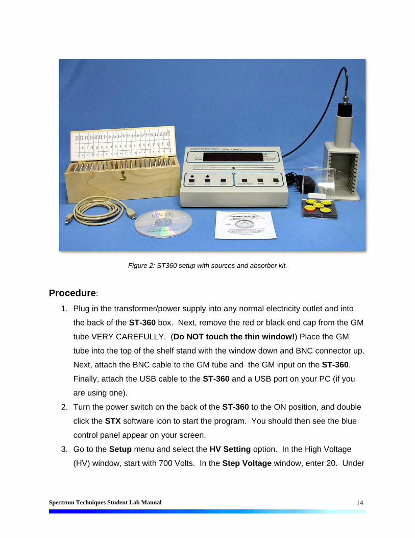
Spectrum Techniques Student Lab Manual
14
Figure 2: ST360 setup with sources and absorber kit.
Procedure:
1. Plug in the transformer/power supply into any normal electricity outlet and into
the back of the ST-360 box. Next, remove the red or black end cap from the GM
tube VERY CAREFULLY. (Do NOT touch the thin window!) Place the GM
tube into the top of the shelf stand with the window down and BNC connector up.
Next, attach the BNC cable to the GM tube and the GM input on the ST-360.
Finally, attach the USB cable to the ST-360 and a USB port on your PC (if you
are using one).
2. Turn the power switch on the back of the ST-360 to the ON position, and double
click the STX software icon to start the program. You should then see the blue
control panel appear on your screen.
3. Go to the Setup menu and select the HV Setting option. In the High Voltage
(HV) window, start with 700 Volts. In the Step Voltage window, enter 20. Under

Spectrum Techniques Student Lab Manual
15
Enable Step Voltage, select On (the default selection is off). Finally, select
Okay.
4. Go under the Preset option and select Time. Enter 30 for the number of
seconds and choose OK. Then also under the Preset option choose Number of
Runs. In the window, enter 26 for the number of runs to make.
5. You should see a screen with a large window for the number of Counts and
Data for all the runs on the left half of the screen. On the right half, you should
see a window for the Preset Time, Elapsed Time, Runs Remaining, and High
Voltage. If not, go to the view option and select Scaler Counts. See Figure 1,
below.
Figure 1, STX setup for GM experiment
6. Make sure no other previous data by choosing the Erase All Data button (with
the red “X” or press F3). Then select the green diamond to start taking data.
7. When all the runs are taken, choose the File menu and Save As. Then you may
save the data file anywhere on the hard drive or onto a floppy disk. The output
file is a text file that is tab delimited, which means that it will load into most

Spectrum Techniques Student Lab Manual
16
spreadsheet programs. See the Data Analysis section for instructions in doing
the data analysis in Microsoft Excel®. Another option is that you may record the
data into your own data sheet and graph the data on the included graph paper.
8. You can repeat the data collection again with different values for step voltage
and duration of time for counting. However, the GM tubes you are using are not
allowed to have more than 1200 V applied to them. Consider this when choosing
new values.
Data Analysis
1. Open Microsoft Excel®. From the File Menu, choose Open. Find the directory
where you saved your data file. (The default location is on the C drive in the
SpecTech directory.) You will have to change the file types to All Files (*.*) to
find your data file that ends with .tsv. Then select your file to open it.
2. The Text Import Wizard will appear to step you through opening this file. You
may use any of the options available, but you need only to press Next, Next, and
Finish to open the file with all the data.
3. To see all the words and eliminate the ### symbols, you should expand the width
of the A and E columns. Place the cursor up to where the letters for the columns
are located. When the cursor is on the line between two columns, it turns into a
line with arrows pointing both ways. Directly over the lines between the A and B
columns and E and F columns, double-click and the columns should
automatically open to the maximum width needed.
4. To make a graph of this data, you may plot it with Excel® or on a sheet of graph
paper. If you choose Excel, the graphing steps are provided.
5. Go the Insert Menu and choose Chart for the Chart Wizard, or select it from the
top toolbar (it looks like a bar graph with different color bars).
6. Under Chart Types, select XY (Scatter) and choose Next. (This default
selection for a scatter plot is what we want to use.)
7. For the Data range, you want the settings to be on “=[your file
name]!$B$13:$C$32”, putting the name you chose for the data file in where [your
file name] is located (do not insert the square brackets or quotation marks). Also,

Spectrum Techniques Student Lab Manual
17
you want to change the Series In option from Rows to Columns. To check to
see if everything has worked, you should have a preview graph with only one set
of points on it. Or you can go to the Series Tab and for X Values should be
“=[your file name]!$B$13:$B$32” and for Y Values should be “=[your file
name]!$C$13:$C$32”. If this is correct, then choose Next again.
8. Next, you are given windows to insert a graph title and labels for the x and y-
axes. Recall that we are plotting Counts on the y-axis and Voltage on the x-
axis. When you have completed that, choose the Legend tab and unmark the
Show Legend Option (remove the check mark by clicking on the box). A legend
is not needed here unless you plotting more than one set of runs together.
9. Next, you are asked to choose whether to keep the graph as a separate
worksheet or to shrink it and insert it onto your current worksheet. This choice is
up to your instructor or you depending on how you want to choose your data
presentation for any lab report.
10. If you insert the chart onto the spreadsheet, adjust its size to print properly. Or
adjust the settings in the Print Preview Option (to the right of print on the top
toolbar).
Conclusions:
Now that you have plotted the GM tube’s plateau, what remains is to determine
an operating voltage. You should choose a value near the middle of the plateau or
slightly left of what you determine to be the center. Again, this will be somewhat difficult
due to the fact that you may not be able to see where the discharge region begins.
Post-Lab Questions:
1. The best operating voltage for the tube = Volts.
2. Will this value be the same for all the different tubes in the lab?
3. Will this value be the same for this tube ten years from now?
4. One way to check to see if your operating voltage is on the plateau is to find the
slope of the plateau with your voltage included. If the slope for a GM plateau is less

Spectrum Techniques Student Lab Manual
18
than 10% per 100 volt, then you have a “good” plateau. Determine where your
plateau begins and ends, and confirm it is a good plateau. The equation for slope is
100
/100%
12
112
VV
RRRslope ,
where R1 and R2 are the activities for the beginning and end points, respectively. V1
and V2 and the voltages for the beginning and end points, respectively. (This equation
measures the % change of the activities and divides it by 100 V.)

Spectrum Techniques Student Lab Manual
19
Data Table for Geiger Plateau Lab
Tube #
Voltage Counts Voltage Counts
Name: Lab Session: Date: Partner:
Don’t forget to hand in this data sheet with a graph of the data.

Spectrum Techniques Student Lab Manual
20
Lab #2: Statistics of Counting
Objective:
In this experiment, the student will investigate the statistics related to
measurements with a Geiger counter. Specifically, the Poisson and Gaussian
distributions will be compared.
Pre-lab Questions:
1. List the formulas for finding the means and standard deviations for the
Poisson and Gaussian distribution.
2. A student in a previous class of the author’s once made the comment, “Why
do we have to learn about errors? You should just buy good and accurate
equipment.” How would you answer this student?
Introduction:
Statistics is an important feature especially when exploring nuclear and particle
physics. In those fields, we are dealing with very large numbers of atoms
simultaneously. We cannot possibly deal with each one individually, so we turn to
statistics for help. Its techniques help us obtain predictions on behavior based on what
most of the particles do and how many follow this pattern. These two categories fit a
general description of mean (or average) and standard deviation.
A measurement counts the number of successes resulting from a given number
of trials. Each trial is assumed to be a binary process in that there are two possible
outcomes: trial is a success or trial is not a success. For our work, the probability of a
decay or non-decay is a constant in every moment of time. Every atom in the source
has the same probability of decay, which is very small (you can measure it in the Half-
life experiment).
The Poisson and Gaussian statistical distributions are the ones that will be used
in this experiment and in future ones. A detailed introduction to those distributions can
be found in Appendix C of this manual.

Spectrum Techniques Student Lab Manual
21
Equipment
Figure 1: Setup for ST360 with sources and absorber kit
Set-up for ST-360 Counter with GM Tube and stand (Counter box, power
supply – transformer, GM Tube, shelf stand, USB cable, and a source holder
for the stand) – Shown in Figure 1.
Radioactive Source (Cs-137 is recommended – the blue source in Figure 1)
Procedure:
1. Setup the equipment as you did in the Experiment #1, and open the computer
interface. You should then see the blue control panel appear on your screen.
2. Go to the Preset menu to preset the Time to 5 and Runs to 150.
3. Take a background radiation measurement. (This run lasts twelve and half minutes
to match the later measurements.)
4. When you are done, save your data onto disk (preferred for 150 data points).

Spectrum Techniques Student Lab Manual
22
5. Repeat with a Cesium-137 source, but reset the Time to 1 and the Number of Runs
to 750 (again will be twelve and a half minutes.)
Data Analysis
1. Open Microsoft Excel®. Import or enter all of your collected data.
2. First, enter all of the titles for numbers you will calculate. In cell G10, enter Mean.
In cell G13, enter Minimum. In cell G16, enter Maximum. In cell G19, enter
Standard Deviation. In cell G22, enter Square Root of Mean. In cell H10, enter
N. In cell I10, enter Frequency. In cell J10, enter Poisson Dist. Finally, in cell
K10, enter Gaussian Dist.
3. In cell G11, enter =AVERAGE(C12:C161) – this calculates the average, or mean.
4. In cell G14, enter =MIN(C12:C161) – this finds the smallest value of the data.
5. In cell G17, enter =MAX(C12:C161) – this finds the largest value of the data.
6. In cell G20, enter =STDEV(C12:C161) – this finds the standard deviation of the data.
7. In cell G22, enter =SQRT(G11) – this takes a square root of the value of the
designated cell, here G11.
8. Starting in cell H11, list the minimum number of counts recorded (same as
Minimum), which could be zero. Increase the count by one all the way down until
you reach the maximum number of counts.
9. In column I, highlight the empty cells that correspond to N values from column H.
Then from the Insert menu, choose function. A window will appear, you will want
to choose the FREQUENCY option that can be found under Statistical (functions
listed in alphabetical order). Once you choose Frequency, another window will
appear. In the window for Data Array, enter C12:C161 (cells for the data). In the
window for Bin Array, enter the cells for the N values in column H. (You can
highlight them by choosing the box at the end of the window.) STOP HERE!! If you
hit OK here, the function will not work. You must simultaneously choose, the
Control key, the Shift key, and OK button (on the screen). Then the frequency for
all of your N values will be computed. If you did not do it correctly, only the first
frequency value will be displayed.
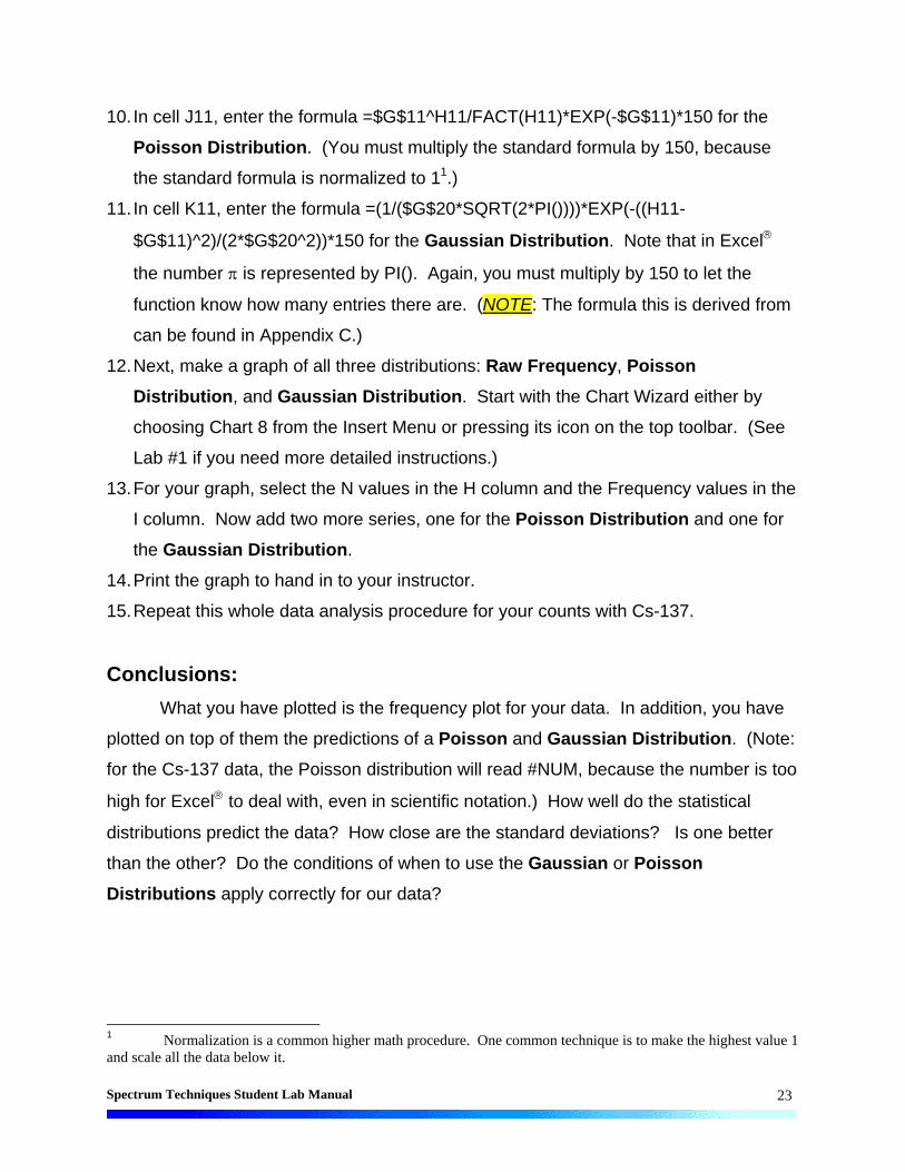
Spectrum Techniques Student Lab Manual
23
10. In cell J11, enter the formula =$G$11^H11/FACT(H11)*EXP(-$G$11)*150 for the
Poisson Distribution. (You must multiply the standard formula by 150, because
the standard formula is normalized to 11.)
11. In cell K11, enter the formula =(1/($G$20*SQRT(2*PI())))*EXP(-((H11-
$G$11)^2)/(2*$G$20^2))*150 for the Gaussian Distribution. Note that in Excel
the number is represented by PI(). Again, you must multiply by 150 to let the
function know how many entries there are. (NOTE: The formula this is derived from
can be found in Appendix C.)
12. Next, make a graph of all three distributions: Raw Frequency, Poisson
Distribution, and Gaussian Distribution. Start with the Chart Wizard either by
choosing Chart 8 from the Insert Menu or pressing its icon on the top toolbar. (See
Lab #1 if you need more detailed instructions.)
13. For your graph, select the N values in the H column and the Frequency values in the
I column. Now add two more series, one for the Poisson Distribution and one for
the Gaussian Distribution.
14. Print the graph to hand in to your instructor.
15. Repeat this whole data analysis procedure for your counts with Cs-137.
Conclusions:
What you have plotted is the frequency plot for your data. In addition, you have
plotted on top of them the predictions of a Poisson and Gaussian Distribution. (Note:
for the Cs-137 data, the Poisson distribution will read #NUM, because the number is too
high for Excel to deal with, even in scientific notation.) How well do the statistical
distributions predict the data? How close are the standard deviations? Is one better
than the other? Do the conditions of when to use the Gaussian or Poisson
Distributions apply correctly for our data?
1 Normalization is a common higher math procedure. One common technique is to make the highest value 1 and scale all the data below it.

Spectrum Techniques Student Lab Manual
24
Post-Lab Questions:
1. Which distribution matches the data with the background counts? How well does
the Gaussian distribution describe the Cs-137 data?
2. Why can’t you get a value for the Poisson distribution with the data from the
Cesium-137 source?
3. How close are the standard deviation values when calculated with the Poisson and
Gaussian Distributions? Is one right (or more correct)? Is one easier to calculate?
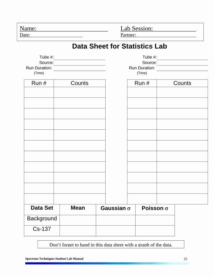
Spectrum Techniques Student Lab Manual
25
Data Sheet for Statistics Lab Tube #: Tube #:
Source: Source:
Run Duration: Run Duration:
(Time) (Time)
Run # Counts Run # Counts
Data Set Mean Gaussian Poisson
Background
Cs-137
Name: Lab Session: Date: Partner:
Don’t forget to hand in this data sheet with a graph of the data.

Spectrum Techniques Student Lab Manual
26
Lab #3: Background
Objective:
The student will investigate background radiation, learn how to measure it, and
compensate for it.
Pre-lab Questions:
1. Name the four natural sources and three man-made sources of background
radiation.
2. Approximately how much background radiation is received by an average
American citizen every year? Is this very high (dangerous)?
Introduction:
In an introductory section of this manual called, What is Radiation, there is a
section that deals with the radiation that is around us everyday of our lives. Normally
we don’t even think about it. However, every living organism contains a radioactive
isotope of carbon, Carbon-14. Whenever you watch TV or look at any object, you must
receive the light waves, which are electromagnetic radiation. Cell phones also transmit
via are electromagnetic radiation. It is all around us and we can’t escape from it. But
we are lucky; because the power and dosage in everyday life is so small there are no
immediate biological effects.
The GM tube is just like a human; it is being bombarded by radiation constantly.
That extra radiation shows up in our GM tube as a count, but it is impossible to
determine the origin of the count as from the radioactive source being investigated or
background. This causes an erroneous sample count. The error can be very high,
especially when the counts are low. Therefore, the background count must be
determined and the sample’s counts must be corrected for it. It is not a difficult process
and is rather straightforward. You find the number of counts with a source present and
without a source present. You subtract the counts obtained without the source from
those obtained with a source, and that should give you the true number of counts from
the source itself.

Spectrum Techniques Student Lab Manual
27
Equipment:
Set-up for ST-360 Counter with GM Tube and stand (Counter box, power
supply – transformer, GM Tube, shelf stand, USB cable, and a source holder
for the stand) – shown in Figure 1.
Figure 1: Setup for ST360 with sources and absorber kit.
Radioactive Source (e.g., Cs-137, Sr-90, or Co-60 – one of the blue, green, or
orange sources shown in Figure 1, respectively)
Procedure:
1. Setup the Geiger Counter as you have in the past two experiments. Set the
Voltage of the GM Tube to its optimal operating voltage (found in the Plateau
Lab). This voltage should be around 900 Volts.
2. Under the Preset Menu, choose Runs. Set the number of runs at 3 and the time
for 5 minutes (or 300 seconds).
3. After the third run has finished, record your data by saving the data to the hard
drive, a floppy disk, or using a data table.

Spectrum Techniques Student Lab Manual
28
4. Insert a radioactive source into one of the (upper) shelves. Complete at least
another 3 runs of 5 minutes each with the radioactive source.
5. Record your data on some scrap paper or a data table, because you will combine
it with the rest of the data later.
Data Analysis:
1. Open Microsoft Excel® and import your data.
2. Beginning in cell A4, fill in the appropriate data for the three runs you performed with
the radioactive source inserted. You do not have to fill in the Time/Date information,
but the run number, high voltage, counts, and elapsed time should all be filled
with data.
3. Go to cell A19, insert the title Average Counts. In cell A20, put the title Average
Background. In cell A21, put the title Average True Counts.
4. In cell B19, enter an equation to calculate the average of the counts with the source
present. In cell B20, enter an equation to calculate the average number of
background counts. In cell B21, enter the equation =B19-B20 to calculate the
number of counts from the source accounting for background radiation.
Conclusions:
As you should see from your data, the background radiation is not high
compared to a radioactive source. You should now know how to deal with background
radiation to obtain a more accurate reading of counts from a radioactive source.
Post-Lab Questions:
1. Is there anyway to eliminate background radiation?
2. What is your prediction for the number of background radiation counts that
your body would receive a day? (Hint: convert from cps or cpm into cpd,
counts per day.) How many counts per year?
3. Are all the background measurements exactly the same number of counts?
Is there a systematic cause for this?
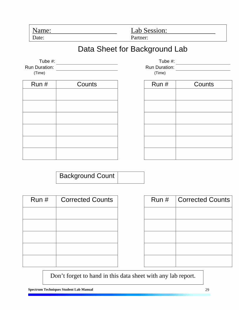
Spectrum Techniques Student Lab Manual
29
Data Sheet for Background Lab
Tube #: Tube #:
Run Duration: Run Duration:
(Time) (Time)
Run # Counts Run # Counts
Background Count
Run # Corrected Counts Run # Corrected Counts
Name: Lab Session: Date: Partner:
Don’t forget to hand in this data sheet with any lab report.

Spectrum Techniques Student Lab Manual
30
Lab #4: Resolving Time
Objective:
The student will determine the resolving time of a GM counter.
Pre-lab Questions:
1. When radiation travels through the window of the GM tube, what happens so that
the tube sends a signal that it has detected a particle?
2. Can the GM counter distinguish between one or more particles when they are
present in the tube at the same time?
Introduction:
When a particle decays and produces radiation, those particles or rays can
produce an ion pair through ionization in the Geiger tube1. The electrons travel to the
anode more quickly than the positive ions travel to the cathode. During the time it takes
the positive ions to reach the cathode, the tube is insensitive to any radiation. During
this time, if a second ionizing ray strikes the tube it will not be detected because the
tube cannot tell there is another electron avalanche present. The Geiger counter only
sees one “big” electron avalanche, until it has been reset after detection. Basically, the
counter cannot produce pulses for more than one particle, because the counter is
“occupied” with the particle that arrives earliest. This phenomenon is sometimes called
coincidence.
As a result of coincidence, the observed counts are always lower than the true
counts. An approximate correction for coincidence is made by adding approximately
0.01% per 100 cpm (counts per minute) to the observed count rate, if it is assumed that
the resolving time2 is about 5 s. True resolving times span a range from a few
microseconds for small tubes to 1000 microseconds for very large detectors. The loss
1 Make sure you read the appendix on the operation of a Geiger-Müller counter. Some aspects on how the Geiger counter works are assumed knowledge for the student. 2 Resolving Time is more commonly referred to as Dead Time by scientists, because in essence the detector is “dead” and cannot detect any other radiation in this time window.

Spectrum Techniques Student Lab Manual
31
of counts is important, especially when there are high count rates involved and the
losses accumulate into large numbers.
In this experiment, you will perform a more accurate analysis of dead time via a
method that uses paired sources. The count rates, or activities, of two sources are
measured individually (r1 and r2) and then together (r3). The paired samples form a disc
cut into two lengthwise. A small quantity of radioactive material is placed on each half
making each a “half-source” of approximately equal strength. A blank disk is used to
duplicate the set-up geometry while using only one half-source. (NOTE: You must keep
the experimental set-up the same or there is a chance that results may change. This is
a common experimental requirement for all sciences.)
Theory:
If we anticipate a counting rate, R, from a radioactive source, then the presence
of coincidence will mean that the rate we actually measure, r, will be less than the
expected value (r < R). If this GM tube has a dead time of T, then the equation for the
true count rate is
R = r + rRT. (1)
This allows us to find an equation to correct our counting rate for dead time
rT
rR
1. (2)
You will have r from your data, and you will be asked to find R. What about T? We look
at our two-source method of data taking, where we measure the activity from two half-
sources, r1 and r2. Then, we measure their combined activity, r3, so we can use this set-
up to our advantage. We expect that the
r1 + r2 = r3 + b (3)
where b is the background counting rate. If each of these counting rates are corrected
for dead time, then Equation (3) becomes
Tr
r
1
1
1 + Tr
r
2
2
1 = Tr
r
3
3
1 + b (4)

Spectrum Techniques Student Lab Manual
32
We do not correct b, because any correction would only be a fraction of a count. Since
the background count rate is negligible, Equation (4) can be changed into the form of a
quadratic equation
r1r2r3T2 – 2r1r2T + r1 + r2 – r3 = 0. (5)
T is on the order of microseconds, so T2 will also be negligible. This allows a very
simple algebraic equation to be solved for T:
21
321
2 rr
rrrT
. (6)
Now, we can solve for R in Equation (2).
Equipment:
Set-up for ST-360 Counter with GM Tube and stand (Counter box, power
supply – transformer, GM Tube, shelf stand, USB cable, and a source holder
for the stand) – shown in Figure 1.
Figure 1: Setup for ST360 with sources and absorber kit.

Spectrum Techniques Student Lab Manual
33
Radioactive Half-Source Kit (3 Half Discs – One Blank and Two of Tl-204) –
shown in Figure 2
Figure 2:Radioactive Half-Source Kit used for Resolving Time determination
Procedure:
1. Setup the Geiger counter as you have in the previous experiments. Set the Voltage
of the GM tube to its optimal operating voltage, which should be around 900 Volts.
2. From the Preset menu, set Runs to zero and set the Time to 60 (You want to
measure counts per minute (cpm), so 60 seconds allows you to convert the number
of counts to cpm).
3. First do a run without a radioactive source. This will determine your background
level. Use two blank disks in the sample tray if they are available.
4. Next, place one of the half-sources on the sample tray with the blank disc. (The
orientation does not matter here but it must be the same throughout the experiment.)
Insert this into one of the upper shelves to take data. Record the number of counts
as r1.

Spectrum Techniques Student Lab Manual
34
5. Replace the blank disc with the second half-source and start a second run. Click on
the green diamond to take data. Record this number of counts as r3.
6. Replace the first half-source with the blank disc and start a third run. Record this
number of counts as r2.
7. Save your data either onto disk or into a data table.
Data Analysis:
1. Open Microsoft Excel® and import your data into it.
2. In cell G9, enter the word Corrected. In cell G10, enter the word Counts.
3. In cells G13-G15, enter the formula to correct for the background. On the data sheet
attached to this lab, the Corrected Counts column is for the final corrected counts,
which means that the correct for resolving time is also done.
4. In cell E2, enter “Resolving Time =”.
5. In cell F2, enter the equation =(G13+G15-G14)/(2*G13*G15).
6. In cell H9, enter the word New and in cell H10 enter Counts.
7. In cells H13-H15, enter the formula =G13/(1-(G13*$F$2)) to correct for resolving
time.
8. In cell I9, enter the words % Counts and in cell I10 enter Added.
9. In cells I13-I15, enter an Excel formula to find the percent of change, which is
100%
measured
measuredcorrected, where the corrected counts are from Column H
and the measured counts are from column H. This value for the percent of the
measurement that was missing due to resolving time will be large, from 20-60% due
to the very active source Tl-204 and the high count rates we are using.
10. Save your worksheet or print it out per your teacher’s instructions.

Spectrum Techniques Student Lab Manual
35
Post-Lab Questions:
1. What is your GM tube’s resolving (or dead) time? Does it fall within the accepted 1
s to 100 s range?
2. Is the percent of correction the same for all your values? Should it be? Why or why
not?

Spectrum Techniques Student Lab Manual
36
Data Sheet for Resolving Time Lab
Tube #: Run Duration:
Source: (Time)
Counts Corr. Counts % Missing
r1:
r2:
r3:
T: Tube #: Run Duration:
Source: (Time)
Counts Corr. Counts % Missing
r1:
r2:
r3:
T:
Name: Lab Session: Date: Partner:

Spectrum Techniques Student Lab Manual
37
Lab #5: Geiger Tube Efficiency
Objective:
The student will determine the efficiency of a Geiger-Muller counter for various
types of radiation.
Pre-lab Questions:
1. How can you determine the activity of a radioactive source? Find the activity of the
three sources you will use in this experiment.
2. Do you expect efficiency to be good or bad for each of your sources? (Consider
real-world effects)
Introduction:
From earlier experiments, you should have learned that a GM tube does not
count all the particles that are emitted from a source, i.e., dead time. In addition, some
of the particles do not strike the tube at all, because they are emitted uniformly in all
directions from the source. In this experiment, you will calculate the efficiency of a GM
tube counting system for different isotopes by comparing the measured count rate to the
disintegration rate (activity) of the source.
To find the disintegration rate, change from microCuries (Ci) to disintegrations
per minute (dpm). The disintegrations per minute unit is equivalent to the counts per
minute from the GM tube, because each disintegration represents a particle emitted.
The conversion factor is:
dpmCiordpmCi 612 1022.211022.21 . (1)
Multiply this by the activity of the source and you have the expected counts per minute
of the source. We will use this procedure to find the efficiency of the GM tube, by using
a fairly simple formula. You want to find the percent of the counts you observe versus
the counts you expect, so you can express this as
CK
rEfficiency
100% . (2)

Spectrum Techniques Student Lab Manual
38
In this formula, r is the measured activity in cpm, C is the expected activity of the source
in Ci, and K is the conversion factor from Equation 1.
Equipment:
Set-up for ST-360 Counter with GM Tube and stand (Counter box, power
supply – transformer, GM Tube, shelf stand, USB cable, and a source holder
for the stand) – shown in Figure 1.
Figure 1 – Setup for ST360 with sources and absorber kit
Radioactive Source (one each of an alpha, beta, and gamma sources – we
recommend Po-210, Sr-90, Co-60 respectively.) – shown in Figure 2.

Spectrum Techniques Student Lab Manual
39
Figure 2 – Kit with one each of an alpha emitter, beta emitter, and gamma emitter
Procedure:
1. Setup the Geiger counter as you have in the previous experiments. Set the Voltage
of the GM tube to its optimal operating voltage, which should be around 900 Volts.
2. From the Preset menu, set Runs to zero and set Preset Time to 60 to measure
activity in cpm.
3. First do a run without a radioactive source to determine your background level.
4. Next, place one of the radioactive sources in the top shelf and begin taking data
5. Repeat this for each of your other two sources. Remember that the first run is a
background number.
6. (OPTIONAL) From the Preset menu, change the Preset Time to 300, and take data
for all three sources again.
7. Save your data to disk or to a data table before exiting the ST-360 program.
Spectrum Techniques Student Lab Manual
40
Data Analysis:
1. Open Microsoft Excel® and import your data into it.
2. In cell E2 enter constant, K = and in cell F2 enter 2.20E6 (or 0.00000220). In cell E3
enter (conversion from Ci to dpm). (To create the , you need to change to the
Symbol font and then simply type the letter m. Don’t forget to switch back to your
original font when you are done.)
3. In cell E5 enter Dead Time = and in cell F6 enter the dead time for your GM tube
found in Lab #4: Resolving Time.
4. In cell G10, enter Activity (Ci). Then cells G13-G17, enter the activities of the
sources used. (Remember to not enter one for the background counts row.)
5. In cell H9 enter Res. Corr. and in cell H10 enter Counts. In cell C13, enter the
formula to correct for resolving time. Copy this formula to cells C14 and C15. Then,
in cell H16, enter the formula again and copy to cells H17 and H18. This should
change the five minute counts to counts per minute, and corrects them for resolving
time.
6. In cell I9 enter Bkgd Corr. and in cell I10 enter Counts. In cell I13, enter the
formula =H13-$C$12. Copy this formula to the other cells. (You may have to adjust
the formula if you took a five minute background count, but don’t forget to convert it
to cpm by dividing by 5.)
7. In cell J10, enter % efficiency. In cell J13, enter the formula for efficiency and copy
it to all the relevant cells.
8. Copy your results to your data table or print out a hard copy if you need to hand one
in attached to a lab report
Conclusions:
Are your results reasonable? How do you know? You should have numbers
above zero but below 10 if you performed the experiment correctly. Answer the post-
lab questions to help you form a conclusion from your results.

Spectrum Techniques Student Lab Manual
41
Post-Lab Questions:
1. Is the efficiency you calculated for each isotope valid only for that isotope?
Explain your answer.
2. If a different shelf is used, will the efficiency change? Explain your answer.
3. The radius of the GM tube’s window is 3.5 cm. The source is 3 cm from the
GM tube. Compare the surface area of a sphere 3 cm from the source to the
area of the GM tube’s window. (Hint: find the ratio) How is this related to this
experiment? Can this tell you if your results are reasonable?
4. (Correlates if five minute and one minute runs were taken.) Are the
efficiencies different? How different? Why?

Spectrum Techniques Student Lab Manual
42
Data Sheet for GM Tube Efficiency Lab
Tube #: Run Duration:
Dead Time: (Time)
Source Counts Corr. Counts Expect. Counts Efficiency
Tube #: Run Duration:
Dead Time: (Time)
Source Counts Corr. Counts Expect. Counts Efficiency
Name: Lab Session: Date: Partner:

Spectrum Techniques Student Lab Manual
43
Lab #6: Shelf Ratios
Objective:
The student will investigate the relationship between the distance and intensity of
radiation. The student will also measure the shelf ratios of the sample holder.
Pre-lab Questions:
1. Does radiation gain intensity or lose intensity as a source gets farther from a
detector?
2. How is radiation emitted from a radioactive source? (Hint: Think of the sun)
Introduction:
Although radiation is emitted from a source in all directions, only a small part
actually enters the tube to be counted. This fraction is a function of the distance, h,
from the point source of radiation to the GM tube. See Figure 1 for a picture of a
“sphere” which represents the radiation emitted radially from the radioactive source. It
can also be observed the small fraction of the “sphere” that will enter the window of
Geiger counter, which is represented by the triangle of sides d and height h. If the
source is moved further away from the tube, the amount of radiation entering the tube
should decrease. This is due to the fact that the triangle’s height will increase, and the
triangle will represent less and less of the “sphere” of radiation.
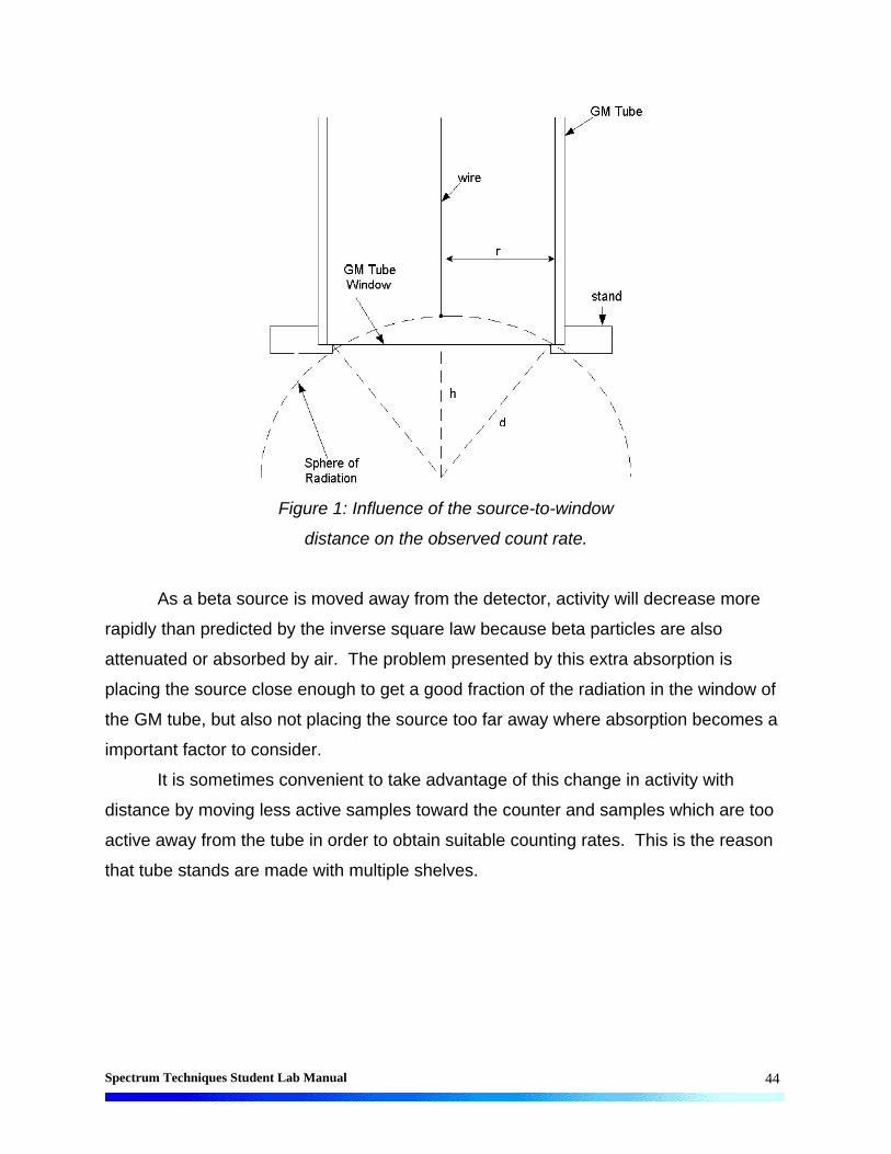
Spectrum Techniques Student Lab Manual
44
Figure 1: Influence of the source-to-window
distance on the observed count rate.
As a beta source is moved away from the detector, activity will decrease more
rapidly than predicted by the inverse square law because beta particles are also
attenuated or absorbed by air. The problem presented by this extra absorption is
placing the source close enough to get a good fraction of the radiation in the window of
the GM tube, but also not placing the source too far away where absorption becomes a
important factor to consider.
It is sometimes convenient to take advantage of this change in activity with
distance by moving less active samples toward the counter and samples which are too
active away from the tube in order to obtain suitable counting rates. This is the reason
that tube stands are made with multiple shelves.
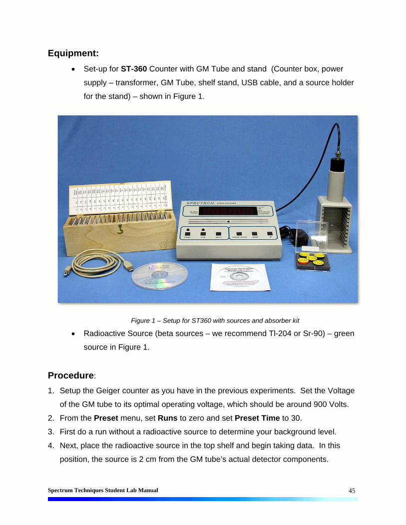
Spectrum Techniques Student Lab Manual
45
Equipment:
Set-up for ST-360 Counter with GM Tube and stand (Counter box, power
supply – transformer, GM Tube, shelf stand, USB cable, and a source holder
for the stand) – shown in Figure 1.
Figure 1 – Setup for ST360 with sources and absorber kit
Radioactive Source (beta sources – we recommend Tl-204 or Sr-90) – green
source in Figure 1.
Procedure:
1. Setup the Geiger counter as you have in the previous experiments. Set the Voltage
of the GM tube to its optimal operating voltage, which should be around 900 Volts.
2. From the Preset menu, set Runs to zero and set Preset Time to 30.
3. First do a run without a radioactive source to determine your background level.
4. Next, place the radioactive source in the top shelf and begin taking data. In this
position, the source is 2 cm from the GM tube’s actual detector components.
Spectrum Techniques Student Lab Manual
46
5. Move the source down one shelf each time and take another run. You should see
the data accumulating in the Data window. After all ten shelves have been used,
save the data onto disk or record in a data table. Remember that the first run is a
background number.
Data Analysis:
1. Open Microsoft Excel® and import your data into it.
2. In Cell E2 enter Dead Time = and in cell F2 enter the dead time for your GM tube
(found in Lab #4).
3. In cell G9 enter Res. Corr. and in cell G10 enter Counts. In cell G13, enter the
formula to correct for resolving, or dead, time and copy this to the rest of the cells
corresponding to counts in column C.
4. In cell H9 enter Bkgd Corr. and in cell H10 enter Counts. In cell H13, enter the
formula to correct for the background, and copy this to the rest of the cells
corresponding to counts in column G.
5. In cell I9 enter Shelf and in cell I10 enter Ratio. In cell I13, enter the formula to
compute the shelf ratio, and copy this to the rest of the cells corresponding to counts
in column H. The shelf ratio is calculated by dividing the number of counts on any
shelf by the number of counts from the second shelf. This should give you a shelf
ratio of 1.00 for the second shelf, which is our reference point.
Conclusions:
You should see a decrease in your values as you move away from the source. If
you do not, this may be caused by statistical fluctuations in your counts. Why?
Post-Lab Questions:
1. Does the shelf ratio depend on the identity of the sample used?
2. If the experiment is repeated with a gamma or alpha source, what differences
would you expect?
3. Why is the second shelf the reference shelf?
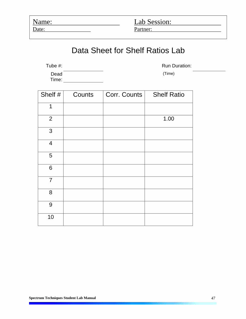
Spectrum Techniques Student Lab Manual
47
Data Sheet for Shelf Ratios Lab
Tube #: Run Duration:
Dead Time:
(Time)
Shelf # Counts Corr. Counts Shelf Ratio
1
2 1.00
3
4
5
6
7
8
9
10
Name: Lab Session: Date: Partner:

Spectrum Techniques Student Lab Manual
48
Lab #7: Backscattering
Objective:
The student will investigate the relationship between absorber material (atomic
number) and backscattering in Part One. In Part Two, the student will investigate the
relationship between absorber thickness and backscattering
Pre-lab Questions:
1. Calculate what percentage of the entire “sphere” surrounding the source does the
GM window occupy.
2. Backscattering does have dependencies on atomic number and on thickness. Does
either one dominant the amount of backscattering versus the other? What kind of
dependence do you predict for each (direct, inverse, inverse square for example –
be descriptive)?
Introduction:
Radiation is emitted from a source in all directions. The radiation emitted within
the angle subtended by the window of the GM tube is the only radiation counted. Most
radiation is emitted away from the tube but it strikes matter. When it does so, the
direction of its path may be deflected. This deflection is known as scattering. Most
particles undergo multiple scattering passing through matter. Beta particles especially
may be scattered through large angles. Radiation scattered through approximately
1800 is said to be backscattered. For Geiger counters, backscatter is the fraction of
radiation emitted away from the GM tube that strikes the material supporting the
sample. It is deflected toward the tube window and is counted.
A beta particle entering matter undergoes a series of collisions with mostly nuclei
and sometimes orbital electrons. A collision between particles does not occur in the
same manner we picture them in the macroscopic world. There are very little contact
collisions, but instead the term, collision, refers to any interaction, coulombic or
otherwise. (A coulombic interaction is an electrical attraction or repulsion that changes
the path of the particle’s motion.) A collision may be elastic or inelastic, but in either

Spectrum Techniques Student Lab Manual
49
case the result is not only a change in direction but usually a decrease in the energy of
the beta particle as well (inelastic).
In the first part of the experiment, we will investigate the effect of the size of the
nucleus on backscattering since this would seem most likely effect the number of
backscattered beta particles. This can be determined by using absorbers as backing
materials. Even though the metal pieces you will use are called absorbers, in this
experiment, they will also be used to deflect radiation upward into the GM tube. To
eliminate any other effects, the absorbers will be the same thickness but different
atomic number (and thus different sized nuclei). In the second part of the experiment,
you will use absorbers of the same material (atomic number) and different thickness.
This is a common experimental technique, fixing one variable and varying another to
investigate each one individually
Normally when we think of thickness, we think of linear thickness that can be
measured in a linear unit such as inches or centimeters. However, in nuclear and
particle physics, thickness refers to areal thickness. This is the thickness of the
absorbers in mg/cm2. The absorptive power of a material is dependent on its density
and thickness, so the product of these two quantities is given as the total absorber
thickness, or areal thickness. We determine areal thickness with the equation:
Density (mg/cm3) X thickness (cm) = Absorber thickness (mg/cm2). (1)
You will determine the dependence that absorber thickness has on backscattering.
Equipment:
Set-up for ST-360 Counter with GM Tube and stand (Counter box, power
supply – transformer, GM Tube, shelf stand, USB cable, and a source holder
for the stand)

Spectrum Techniques Student Lab Manual
50
Figure 1 – Setup for ST360 with sources and absorber kit
Radioactive Source (THIN* beta emitter)
Part I: Backscatter Absorber Kit – Plastic (poly-carbonate), Aluminum,
Copper, Tin, Lead, and “an unknown” Discs
Part II: (Regular) Absorber Kit – the Aluminum and Lead pieces will be used.
(Shown in Figure 1.)
Procedure:
Part I – Atomic Number Dependence
1. Setup the Geiger counter as you have in the previous experiments. Set the Voltage
of the GM tube to its optimal operating voltage, which should be around 900 Volts.
2. From the Preset menu, set Runs to zero and set Preset Time to 60.
3. First do a run without a radioactive source to determine your background level.
4. Next, place the radioactive source in the second shelf from the top and take data.
* A thin source is required to reduce self-absorption by the source. This enables beta particles sent downward that are scattered back up toward the GM tube may pass through the source again.

Spectrum Techniques Student Lab Manual
51
5. Place an absorber piece, or disk, in the source holder and place the source directly
on top of it.
6. Repeat this for all of the various absorbers (different materials) including the
unknown.
7. Record the data to a file on disk or into a data table.
Part II – Thickness Dependence
1. Setup the Geiger counter as you have in the previous experiments. Set the Voltage
of the GM tube to its optimal operating voltage, which should be around 900 Volts.
2. From the Preset menu, set Runs to zero and set Preset Time to 60.
3. First do a run without a radioactive source to determine your background level. (Do
not repeat if this is part is being performed in the same lab period as Part I.)
4. Next, place the radioactive source in the second shelf from the top and begin taking
data.
5. Place the source directly on top of one of the absorbers. Take data by clicking on
the green diamond.
6. Place the source on a different absorber and insert into the second shelf. Click on
the green diamond to begin taking data.
7. Repeat for at least three other absorber thicknesses.
8. Record the data to a file on disk or into a data table.
Data Analysis:
Part I – Atomic Number Dependence
1. Open Microsoft Excel® and import your data into it.
2. In cell E2, enter Dead Time = and in cell F2 enter the dead time determined for your
GM tube.
3. In cell G9 enter Dead Corr. and in cell G10 enter Counts. In cell G13, enter a
formula to correct for dead time. Copy this down for the cells that have counts in
column C.
4. In cell H9 enter Corrected and in cell H10 enter Counts. In cell H13, enter a
formula to correct for background counts. Copy this down for the cells that have

Spectrum Techniques Student Lab Manual
52
counts in column G. Is background significant? Can you back up your answer
numerically?
5. In cell I9 enter Atomic and in cell I10 enter Number. In cell I13 and below, enter the
atomic numbers for the absorbers you used to get obtain the corresponding counts.
(Plastic is poly-carbonate** – Z = 6, Aluminum – Z = 13, Copper – Z = 29, Tin – Z =
50, and Lead – Z = 82)
6. To double-check the general result of our data that we will graph below, we will
calculate the percentage of counts that were due to backscattering and compare that
to the Z values. To calculate the percent of counts from backscattering, use the
following formula 100%
o
o
r
rrback , where r is the corrected count rate (cpm)
and ro is the count rate without any absorber present. To do this in Excel, in cell J9
enter Percent and cell J10 Backscatt. In cell J13, enter the formula
=((H13-$H$13)/$H$13)*100. This should give 0 for cell J13 but not for the rest.
7. Next, make a graph of Corrected Counts vs. Atomic Number. Start with the Chart
Wizard either by choosing Chart from the Insert Menu or pressing its icon on the top
toolbar.
9. Select the Atomic Number values in the I column and Corrected Counts values in
the H column.
10. Fill in the Chart Title, Value (X) Axis, and Value (Y) Axis windows with appropriate
names and units (if applicable) for those items.
11. Choose whether you want to view your graph as a separate worksheet as your data,
or you wish to see a smaller version of the graph with the data.
12. Adjust the size of the graph for your preference (or the instructor’s). You may also
wish to adjust the scales on one or more of the axes. Again, this is a preference
issue.
13. Right click on one of the data points and from the menu that appears, choose Add
Trendline. Make sure that the Linear option is chosen (should be darkened). Then
click on the Options tab and check the boxes for Display equation on chart and
* * Plastic is effectively carbon because that is the dominating element in this material.

Spectrum Techniques Student Lab Manual
53
Display R-squared value on chart. This will make the equation of the best fit line
appear as well as a number that represents the percent of linearity of the data.
Part II – Thickness Dependence
1. Open Microsoft Excel® and import
2. In cell E2, enter Dead Time = and in cell F2 enter the dead time determined for your
GM tube.
8. In cell G9 enter Dead Corr. and in cell G10 enter Counts. In cell G13, enter a
formula to correct for dead time. Copy this down for the cells that have counts in
column C.
9. In cell H9 enter Corrected and in cell H10 enter Counts. In cell H13, enter a
formula to correct for background counts. Copy this down for the cells that have
counts in column G.
3. In cell I9 enter Thickness and in cell I10 enter (in). In cell I13 and below, enter the
thickness of the absorbers (0.32, 0.063, or 0.125 inches) for the aluminum and
lead***.
4. Calculate the percentage of counts that were due to backscattering. In cell J9 enter
Percent and cell J10 Backscatt. In cell J13, enter the same formula as for Part I for
percent of backscattering. This should give 0 for cell J13 but not for the rest.
5. Next, make a graph of Corrected Counts vs. Thickness. Start with the Chart Wizard
either by choosing Chart from the Insert Menu or pressing its icon on the top toolbar.
6. Select the Thickness values in the I column and Corrected Counts values in the H
column.
7. Fill in the Chart Title, Value (X) Axis, and Value (Y) Axis windows with appropriate
names and units (if applicable) for those items.
8. Choose whether you want to view your graph as a separate worksheet as your data,
or you wish to see a smaller version of the graph with the data.
* ** Lead has an absorber that is 0.064 inches thick instead of the listed 0.063 inches. Make sure you enter it correctly.

Spectrum Techniques Student Lab Manual
54
9. Adjust the size of the graph for your preference (or the instructor’s). You may also
wish to adjust the scales on one or more of the axes. Again, this is a preference
issue.
10. Right click on one of the data points and from the menu that appears choose Add
Trendline. Make sure that the Linear option is chosen (should be darkened). Then
click on the Options tab and check the boxes for Display equation on chart and
Display R-squared value on chart. This will make the equation of the best-fit line
appear as well as a number that represents the percent of linearity of the data.
Conclusions:
What is your conclusion about the dependence of backscattering on atomic
number? How about on thickness?
Post-Lab Questions:
1. Justify your answers to the questions about the dependences of
backscattering.
2. Do your % backscattering calculations confirm your results?
3. What element (or material) is the unknown absorber?
4. What would be the predicted count rate for a uranium disk of the same size
as those used in Part I? How about if it was ¼ in. thick (qualitative answer,
higher or lower)? Show your work and explain any reasoning.

Spectrum Techniques Student Lab Manual
55
Data Sheet for Backscattering Lab
Tube #: Run Duration:
Dead Time: (Time)
Part I
Element (Z) Counts Corr. Counts % Backscat.
Name: Lab Session: Date: Partner:
Name: Lab Session: Date: Partner:
Don’t forget to hand in a graph of the data with this table.

Spectrum Techniques Student Lab Manual
56
Data Sheet for Backscattering Lab
Tube #: Run Duration:
Dead Time: (Time)
Part II
Thickness Counts Corr. Counts % Backscat.
Don’t forget to hand in a graph of the data with this table.

Spectrum Techniques Student Lab Manual
57
Lab #8: Inverse Square Law
Objective:
The student will verify the inverse square relationship between the distance and
intensity of radiation.
Pre-lab Questions:
1. Write a general mathematical expression for an inverse square law.
2. What are other examples of inverse square laws?
Introduction:
As a source is moved away from the detector, the intensity, or amount of
detected radiation, decreases. You may have observed this effect in a previous
experiment, Shelf Ratios Lab. If not, you have observed a similar effect in your life.
The farther you move away from a friend, the harder it is to hear them. Or the farther
you move away from a light source, the harder it is to see. Basically, nature provides
many examples (including light, sound, and radiation) that follow an inverse square law.
What an inverse square law says is that as you double the distance between
source and detector, intensity goes down by a factor of four. If you triple the distance,
intensity would decrease by a factor of nine. If you quadruple the distance, the intensity
would decrease by a factor of 16, and so on and so on. As a result, if you move to a
distance d away from the window of the GM counter, then the intensity of radiation
decreases by a factor 1/d2.
Equipment:
Set-up for ST-360 Counter with GM Tube and stand (Counter box, power
supply – transformer, GM Tube, shelf stand, USB cable, and a source holder
for the stand) – shown in Figure 1.
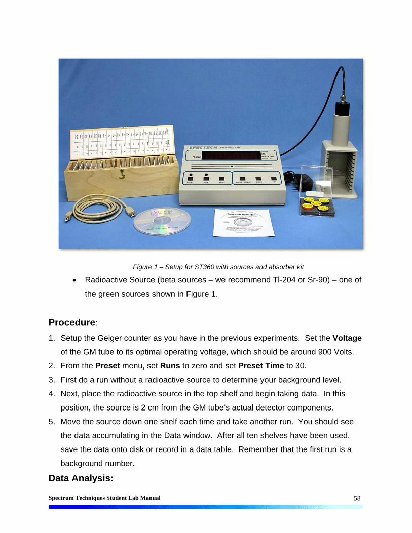
Spectrum Techniques Student Lab Manual
58
Figure 1 – Setup for ST360 with sources and absorber kit
Radioactive Source (beta sources – we recommend Tl-204 or Sr-90) – one of
the green sources shown in Figure 1.
Procedure:
1. Setup the Geiger counter as you have in the previous experiments. Set the Voltage
of the GM tube to its optimal operating voltage, which should be around 900 Volts.
2. From the Preset menu, set Runs to zero and set Preset Time to 30.
3. First do a run without a radioactive source to determine your background level.
4. Next, place the radioactive source in the top shelf and begin taking data. In this
position, the source is 2 cm from the GM tube’s actual detector components.
5. Move the source down one shelf each time and take another run. You should see
the data accumulating in the Data window. After all ten shelves have been used,
save the data onto disk or record in a data table. Remember that the first run is a
background number.
Data Analysis:
Spectrum Techniques Student Lab Manual
59
1. Open Microsoft Excel® and import your data into it.
2. In cell E2, enter Dead Time = and in cell F2 enter the dead time determined for your
GM tube.
3. Go cell G9 and insert the word True. Go to cell G10 and insert the word Counts. In
cell H10, insert Distance (cm). In cell I10, insert Distance (m). In cell J10, insert
1/d^21.
4. In cells G13 down to G14, insert a formula to correct for dead time and background.
(may need additional column).
5. In cell H13, insert the distances in centimeters. They should begin with 2 and
increase by one until 11 is reached.
6. In cell I13, insert the formula to convert the distance from centimeters to meters.
Copy this formula in each cell from I14 down to I22.
7. In cell J13, insert the formula =1/(I13*I13) or =1/(I13^2). Either form gets you the
inverse square of the distance. Copy this formula in the cells down from J14 to J22.
8. Next, make a graph of Counts vs. 1/d2. Start with the Chart Wizard either by
choosing Chart from the Insert Menu or pressing its icon on the top toolbar.
9. Choose the True Counts values in the H column and the 1/d2 values in the J column.
10. Fill in the Chart Title, Value (X) Axis, and Value (Y) Axis windows with appropriate
names and units (if applicable) for those items. Recall that Counts are a unitless
quantity.
11. Position your cursor directly over one of the data points on your graph. Then click
the right button on the mouse and watch a small menu appear. Choose the Add
Trendline option. You may click OK here or if you want more information choose
the Options Tab. There you may click in the boxes for Display Equation on Chart
(for the equation of the line in slope-intercept form to appear on the graph) or on
Display R-squared Value on Chart (this gives a decimal representation of the
percentage completely linear the data is).
Conclusions:
Use your graph to determine if the data does indeed obey inverse square law.
1 The carrot, ^, is the computer programming way of indicating exponent or power.

Spectrum Techniques Student Lab Manual
60
Post-Lab Questions:
1. Does your data follow Excel®’s best fit line? If not, why?
2. Does this verify the inverse square law? Explain?
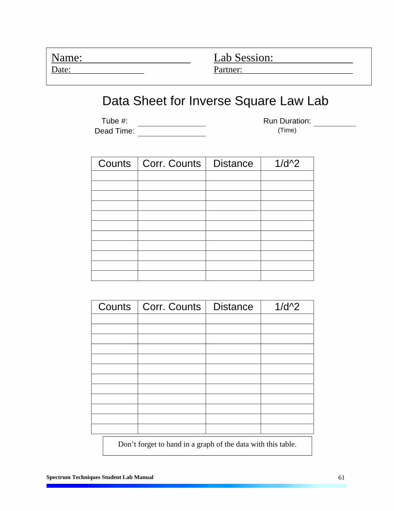
Spectrum Techniques Student Lab Manual
61
Data Sheet for Inverse Square Law Lab
Tube #: Run Duration:
Dead Time: (Time)
Counts Corr. Counts Distance 1/d^2
Counts Corr. Counts Distance 1/d^2
Name: Lab Session: Date: Partner:
Don’t forget to hand in a graph of the data with this table.

Spectrum Techniques Student Lab Manual
62
Lab #9: Range of Alpha Particles
Objective:
The student will determine the range of an alpha particle in air, and consequently
the alpha particle’s energy.
Pre-lab Questions:
1. What is an alpha particle? How and why are they emitted?
2. What everyday material can block alpha particles?
3. Do you predict the range to be long or short? Why?
Introduction:
We know that particles that enter matter lose their energy1 via collisions with
atoms in the matter. So, a natural question would be, how far will the particle travel in
the matter before it loses all of its energy? This quantity is called the range of a
particle, and depends on the type of material, particle type, and its energy. Normally,
we assume that the energy loss is continuous (particle loses some energy for each
amount of distance it travels); the range will be a certain distance for the same particles
with identical initial energies passing through the same type of material. In this
experiment, you will look at alpha particles passing through air.
The alpha particle () is a helium ion (+2), which is composed of two protons (p)
and two neutrons (n). Ramsay and Soddy observed that helium is constantly being
produced from radium and that radioactive minerals invariably contain helium.
Rutherford and Royds later showed that alpha particles form neutral helium atoms when
they lose their kinetic energy. In the process, each alpha particle gains two electrons
from the surrounding material.
Alpha particles emitted from a particular species of nucleus are mono-energetic;
alphas from the same species have the same energy. The energy of most alphas falls
1 When dealing with particles, we ignore potential energies from bonding mainly because the size is so small. The term energy refers solely to the kinetic energy of the particle.

Spectrum Techniques Student Lab Manual
63
in the range between 3 and 8 MeV. By comparison, chemical reactions have energies
of 5 to 30 eV per molecule.
The velocity of an alpha particle upon emission from the nucleus depends upon
the radioelement of its origin. The alpha particle has great ionizing power, but very little
penetrating power. (If it enters the GM tube, then it will ionize the gas and be detected
unless it is the dead time.) Its energy is approximated by its range in air in the equation:
5.1 RE , (1)
where R is the range in air of the alpha particle in centimeters and E is the energy of the
alpha particle in MeV.
Equipment:
Set-up for ST-360 Counter with GM Tube and stand (Counter box, power
supply – transformer, GM Tube, shelf stand, USB cable, and a source holder
for the stand) – shown in Figure 1.
Figure 1 – Setup for ST360 with sources and absorber kit
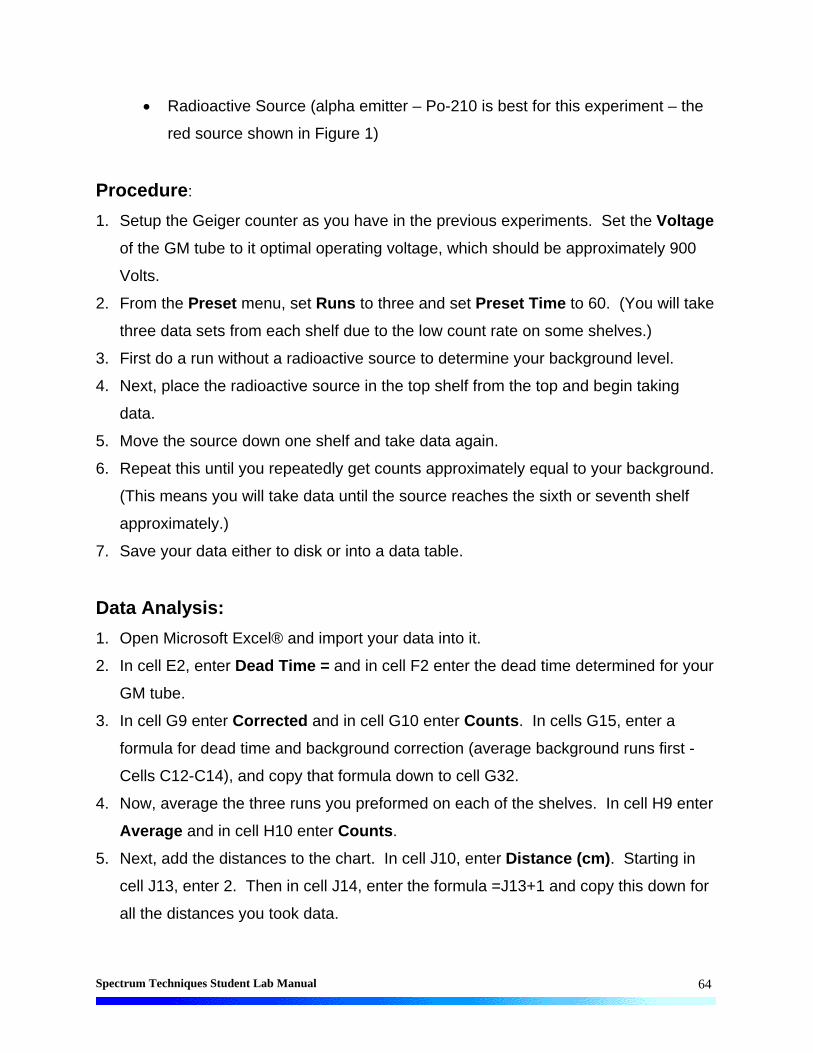
Spectrum Techniques Student Lab Manual
64
Radioactive Source (alpha emitter – Po-210 is best for this experiment – the
red source shown in Figure 1)
Procedure:
1. Setup the Geiger counter as you have in the previous experiments. Set the Voltage
of the GM tube to it optimal operating voltage, which should be approximately 900
Volts.
2. From the Preset menu, set Runs to three and set Preset Time to 60. (You will take
three data sets from each shelf due to the low count rate on some shelves.)
3. First do a run without a radioactive source to determine your background level.
4. Next, place the radioactive source in the top shelf from the top and begin taking
data.
5. Move the source down one shelf and take data again.
6. Repeat this until you repeatedly get counts approximately equal to your background.
(This means you will take data until the source reaches the sixth or seventh shelf
approximately.)
7. Save your data either to disk or into a data table.
Data Analysis:
1. Open Microsoft Excel® and import your data into it.
2. In cell E2, enter Dead Time = and in cell F2 enter the dead time determined for your
GM tube.
3. In cell G9 enter Corrected and in cell G10 enter Counts. In cells G15, enter a
formula for dead time and background correction (average background runs first -
Cells C12-C14), and copy that formula down to cell G32.
4. Now, average the three runs you preformed on each of the shelves. In cell H9 enter
Average and in cell H10 enter Counts.
5. Next, add the distances to the chart. In cell J10, enter Distance (cm). Starting in
cell J13, enter 2. Then in cell J14, enter the formula =J13+1 and copy this down for
all the distances you took data.

Spectrum Techniques Student Lab Manual
65
6. Use that number as R in Equation (1) to find the energy of your alpha particles.
Compare this value of E to the expected value, 5.34 MeV, by finding the percent
error. Record these values either in the spreadsheet or on your data sheet.
100%
ltheoretica
ltheoreticameasurederror (2)
OPTIONAL:
7. A graph is very tricky here because of lack of measurements below 2 cm. In
addition, you would like measurements in increments less than 1 cm. Look at your
data. Where is there a sudden fall-off in the counts per minute (going from
thousands to tens)? Where does the data dip below the x-axis? Use extrapolation
to guess where these two situations occur (i.e., 2.7 cm because it fell in-between 2
cm and 3 cm but seems closer to 3 cm). Average these two numbers and that gives
the mean range of your alpha particles.
8. Make a graph of Corrected Counts per Minute vs. Distance. Start with the Chart
Wizard either by choosing Chart from the Insert Menu or pressing its icon on the
top toolbar.
9. Use the Average Counts in column I and Distance in column J columns of data.
10. Fill in the Chart Title, Value (X) Axis, and Value (Y) Axis windows with appropriate
names and units (if applicable) for those items.
11. Choose whether you want to view your graph as a separate worksheet as your data,
or you wish to see a smaller version of the graph with the data. Click Finish when
you have chosen one or the other.
Conclusions:
What you should see in a graph of your data (if you made one) is that as the data
approaches the range, it does not drop immediately to the background level directly at
the range value. Instead, the curve slopes down over a certain interval of distances.
This is because our original assumption of energy loss being continuous is not quite
accurate. Not every identical particle will have identical energy loss. That is because
every particle suffers a different number of collisions when passing through matter and

Spectrum Techniques Student Lab Manual
66
thus have slightly different energy losses. This means that energy loss is statistical in
nature.
If you measure an ensemble (or group) of identical particles passing through the
same sample, then you will a statistical distribution of ranges centered about some
mean value, the mean range. This phenomenon is known as range straggling. This
means some alpha particles are stopped with less air than others, because of the
difference in the number of collisions it has with air molecules.
Figure 2: Alpha particle range straggling is shown. The intensity of alpha
particles drops off over a small range and not immediately at one value.
An example of a plot of alpha range straggling is shown in Figure 2. You can see
that at that point the counts first drop off sharply to the left of the mean range, which is
one point you can identify on the graph from your data. Then there is a sudden drop off
to zero to the right of the mean range where the counts above background are zero.
This is the other point you should found. Then, the point in the point in the middle of
these other two will be your mean range.
Post-Lab Questions:
1. Compare your results of range and energy to those values that can be found
in a handbook (see Figure 3). Results?

Spectrum Techniques Student Lab Manual
67
Figure 3: Plot of Alpha particle range versus energy in MeV.
2. How far away should a person stand to not receive any alpha particles that
are emitted from a nucleus at 8 MeV?
3. How reliable is your data? In other words, is the percent error high? (Explain
why you think it is high) If it is high, is that OK? Why?

Spectrum Techniques Student Lab Manual
68
Data Sheet for Alpha Range Lab
Tube #: Run Duration:
Dead Time: (Time)
Shelf Counts Corr. Counts d (cm)
Fall off starts about: Cm E = R + 1.5
Fall off ends about: Cm E = MeV
Center of Fall off: Cm Lit. Value: E= MeV
% Error =
Name: Lab Session: Date: Partner:
Don’t forget to hand in a graph of the data with this table.

Spectrum Techniques Student Lab Manual
69
Lab #10: Absorption of Beta Particles
Objective:
The student will investigate the attenuation of radiation via the absorption of beta
particles.
Pre-lab Questions:
1. How does activity of a source vary with distance?
2. How do you predict activity will vary with increasing absorber thickness, when an
absorber is placed between the source and window of the GM tube?
Introduction:
Beta particles are electrons that are emitted from an atom when a neutron
decays by the weak force. The neutron (n) becomes a proton (p), an electron (e-), and
an anti-neutrino ( )1. When an electron originates in the nucleus, it is called a beta
particle.
epn (1)
Unlike alpha particles that are emitted from the nucleus with the same energy (~5
MeV), beta particles are emitted with a range of energies between 0 MeV and the
maximum energy for a given radioactive isotope. The velocity of a beta particle is
dependent on its energy, and velocities range from zero to about 2.9 x 10⁸ m/s, nearly
the speed of light. So the beta particles do not all have the same kinetic energy and
thus they do not all have the same range. When the range varies over different values,
this is called range straggling. It represents the different energy losses all of the beta
particles have given their different initial values. Figure 1 shows a typical absorption
curve for beta particles, which illustrates the range straggling.
1 The purpose of the anti-neutrino’s creation is to carry off extra energy and momentum for the conservation of those quantities.

Spectrum Techniques Student Lab Manual
70
Figure 1: Typical absorption curve for beta particles. Plot is
of intensity (activity) vs. absorber thickness (x)
Equipment:
Set-up for ST-360 Counter with GM Tube and stand (Counter box, power
supply – transformer, GM Tube, shelf stand, USB cable, and a source holder
for the stand) – shown in Figure 2.
Figure 2: Setup for ST360 with sources and absorber kit.

Spectrum Techniques Student Lab Manual
71
Radioactive Source (beta emitter – any green source shown in Figure 2)
Procedure:
1. Setup the Geiger counter as you have in previous experiments. Set the Voltage of
the GM tube to its optimal operating voltage, which should be around 900 Volts.
2. From the Preset menu, set Runs to zero and set Preset Time to 60.
3. First do a run without a radioactive source to determine your background level.
4. Next, place the radioactive source in the second shelf from the top and begin taking
data.
5. Place an absorber piece in the top shelf and take another run of data.
6. Repeat this a minimum of 5 more times with absorbers of increasing thickness.
Data Analysis:
1. Open Microsoft Excel® and import your data into it.
2. In cell F6, enter Dead Time = and in cell G6 enter the dead time determined for your
GM tube.
3. In cell G9, enter Thickness and in cell G10 enter mg/cm2. Then starting in cell
G13, enter the thickness for the absorbers used. For cell G13, it should be zero (no
absorber used). In column F, under Notes, it may be convenient to enter the letters
associated with the absorbers you used.
4. In cell H9 enter Dead Corr. and in cell H10 enter Counts. Then starting in cell H13,
enter a formula to correct for the dead time of the GM counter. Copy this formula
down the column for all the data you collected.
5. In cell I9 enter Corrected and in cell I10 enter Counts. Then starting in cell I13,
enter a formula to correct for the background of the GM counter. Copy this formula
down for all the data you have.
6. In cell J9 enter Natural Log and in cell J10, enter of Counts. Then in cell J13, enter
the formula =LN(I13) and copy this formula down for all the data you have.
7. Next, make a graph of Corrected Counts vs. Thickness. Start with the Chart
Wizard either by choosing Chart from the Insert Menu or pressing its icon on the
top toolbar.

Spectrum Techniques Student Lab Manual
72
8. Select the Thickness values in the G column and the Corrected Counts values in
the I column.
9. Fill in the Chart Title, Value (X) Axis, and Value (Y) Axis windows with appropriate
names and units (if applicable) for those items.
10. Add a trendline to the graph. The x-intercept represents the extrapolated range.
Conclusions:
You should be able to characterize the relationship between beta particle activity
and absorber thickness.
Post-Lab Questions:
1. Is your data linear? If not, what type of behavior does it exhibit?
2. What is the slope for your data? How did you obtain it?
3. What is the range of the beta particles, so that all of them stop?
4. Bremmsstrahlung (German for braking radiation) is the name given to x-rays
produced by beta particles reacting with matter. Was any Bremmsstrahlung
produced during the experiment? Can it minimized?

Spectrum Techniques Student Lab Manual
73
Data Sheet for Beta Absorption Lab
Tube #: Run Duration:
Dead Time: (Time)
Counts Corr. Counts Thickness ln (Counts)
Name: Lab Session: Date: Partner:
Don’t forget to hand in a graph of the data with this table.

Spectrum Techniques Student Lab Manual
74
Lab #11: Beta Decay Energy
Objective:
The student will determine the maximum energy of decay of a beta particle.
Pre-lab Questions:
1. What is the decay mechanism for beta decay? Why are there three decay
products?
2. What are the units of thickness for an absorber?
3. Why shouldn’t a beta source be placed below the third shelf? Or above the second
shelf?
Introduction:
When beta particles are emitted from a nucleus, they are emitted over a wide
range of energies. Recall that this is different from alpha particles, which are emitted
monoenergetically. The maximum energy of the emitted beta particles is a
characteristic signature for different radioisotopes.
In this experiment, you will find the range of beta particles by measuring their
attenuation1 with absorbers and extrapolating the absorption curve. The range R will
then be substituted into the formula
212.084.1 RE (1)
where R is in g/cm2. (Note that the units for R are not the same as the absorber
thicknesses. You must convert at the end.) See Figure 1 for an example of an energy
curve for beta particles.
1 Attenuation is a term used for the exponential decrease of a quantity.

Spectrum Techniques Student Lab Manual
75
Figure 1: Typical plot of beta particle energy curve.
The spectrum is not linear and “tails” off at high energy, which means that there
are very few beta particles (This effect is seen with the phenomenon of range
straggling, which was observed in the absorption curve in the previous experiment.)
The reason is that most of the beta particles cannot penetrate the absorber and most of
the counts are background counts. Thus, one must assume linearity and extrapolate
the line to the x-axis. There are two options to finding this x-intercept. The first is to find
an equation for the best-fit line of the data in slope-intercept form, y = mx + b. Then set
y = 0 and solve for the x value, since the x-intercept is the point on the line where the y
– coordinate is zero. The second method is to take a copy of the plot and use a rule to
continue the linear part of the data through the x-axis and finding that point.
Equipment:
Set-up for ST-360 Counter with GM Tube and stand (Counter box, power
supply – transformer, GM Tube, shelf stand, USB cable, and a source holder
for the stand) – shown in Figure 2.
Radioactive Source (beta sources – Sr-90 or Tl-204 are recommended) –
green source shown in Figure 2.

Spectrum Techniques Student Lab Manual
76
Figure 2: Setup for ST360 with sources and absorber kit.
Procedure:
1. Set up the Geiger counter as you have in the previous experiments. Set the
Voltage of the GM tube to its optimal operating voltage, which should be around 900
Volts.
2. From the Preset menu, set Runs to three and set Preset Time to 60.
3. First do a run without any absorber and with a radioactive source. Place the source
in the second shelf and click the green diamond to begin taking data. No
background reading is taken because 204Tl and 90Sr are relatively strong beta
sources (high count rates) and the background will be negligible (20-40 cpm).
4. Next, place the first absorber in the top shelf, directly above the source, and begin
taking data.
5. Change your absorber each time for as many absorbers as the instructor gives to
you. You should see the data accumulating in the Data window. After all the
absorbers have been used, save the data onto disk or record in a data table.

Spectrum Techniques Student Lab Manual
77
Data Analysis:
1. Open Microsoft Excel® and import your data into it.
2. In cell E2 enter Dead Time = and then in cell F2 enter the value for your GM tube’s
resolving time.
3. In cell G9 enter Corrected and in cell G10 enter Counts. Next, in cell G13, enter a
formula to correct for your data for resolving time. Copy this formula down for all the
cells that should contain data.
4. In cell H9 enter Thickness and in cell H10 enter (mg/cm2). Then, in column H
beginning with cell 12, enter the thickness values you used taking data.
5. In cell I9 enter Log of and in cell I10 enter Activity. Next, in cell I13, enter the
formula =LOG(G13) to calculate the logarithm (base 10) of your data. Copy this
formula down for all the cells that should contain data. Taking the logarithm of the
data substitutes for plotting your data on semi-log paper.
6. Next, make a graph of Log of Activity vs. Thickness. Start with the Chart Wizard
either by choosing Chart from the Insert Menu or pressing its icon on the top toolbar.
7. Select the thickness values in the H column and the Log of Activity values in the I
column.
8. Fill in the Chart Title, Value (X) Axis, and Value (Y) Axis windows with appropriate
names and units (if applicable) for those items.
9. Add a trendline to your graph.
10. In cell A34, copy the equation shown for the best-fit line in your graph. Then, set y =
0 and solve for x. This breaks down to dividing the negative of the y-intercept by the
value for the slope (should be negative). Take the value for x and divide it by 1000,
because your answer was in mg/cm2. But to use the equation given earlier for
maximum energy, you need x in units of g/cm2. This is your value of the range R of
a beta particle emitted from your source.
11. Then plug your value for R into 212.084.1 RE and get a value for E. Place this
value in cell B36. In cell A36, enter E =.
12. In cell A38 enter True Value for E =. Then in cell B38, enter the literature value for
your source. (Sr-90 has E = 0.546 MeV and Tl-204 has E = 0.7634 MeV.)

Spectrum Techniques Student Lab Manual
78
13. In cell A40 enter Percent Error =. In cell B40, enter the formula =((ABS(B36-
B38))/B38)*100. This formula represents the formula
100%
true
measuredtrueerror . (2)
Conclusions:
You should have found the value for the maximum energy of a beta particle from
your source and the percent error of this result when compared to the literature value.
However, this percent error is not a good way to determine experimental error. As
discussed in a previous lab, the best way to determine error is to use the standard
deviation. So, calculate for your value of E – you will have to use propagation of
errors. (OPTIONAL)
Post-Lab Questions:
1. Does your data follow Excel’s® best fit line? If not, why?
2. Why does the data fluctuate so much at high absorber values, especially
those above 1400 mg/cm2? How can this be handled in the data analysis
stage?
3. Is your result for E accurate? Is it still a good result even if it is not exactly the
same as the literature value?

Spectrum Techniques Student Lab Manual
79
Data Sheet for Beta Energy Lab
Tube #: Run Duration:
Dead Time: (Time)
Counts Corr. Counts Thickness ln (Counts)
Equation for line: y=
For y=0, x= mg/cm^2
Conversion x= g/cm^2 (This is the range)
Use E = 1.84*R+0.212
E= MeV
Name: Lab Session: Date: Partner:
Don’t forget to hand in a graph of the data with this table.
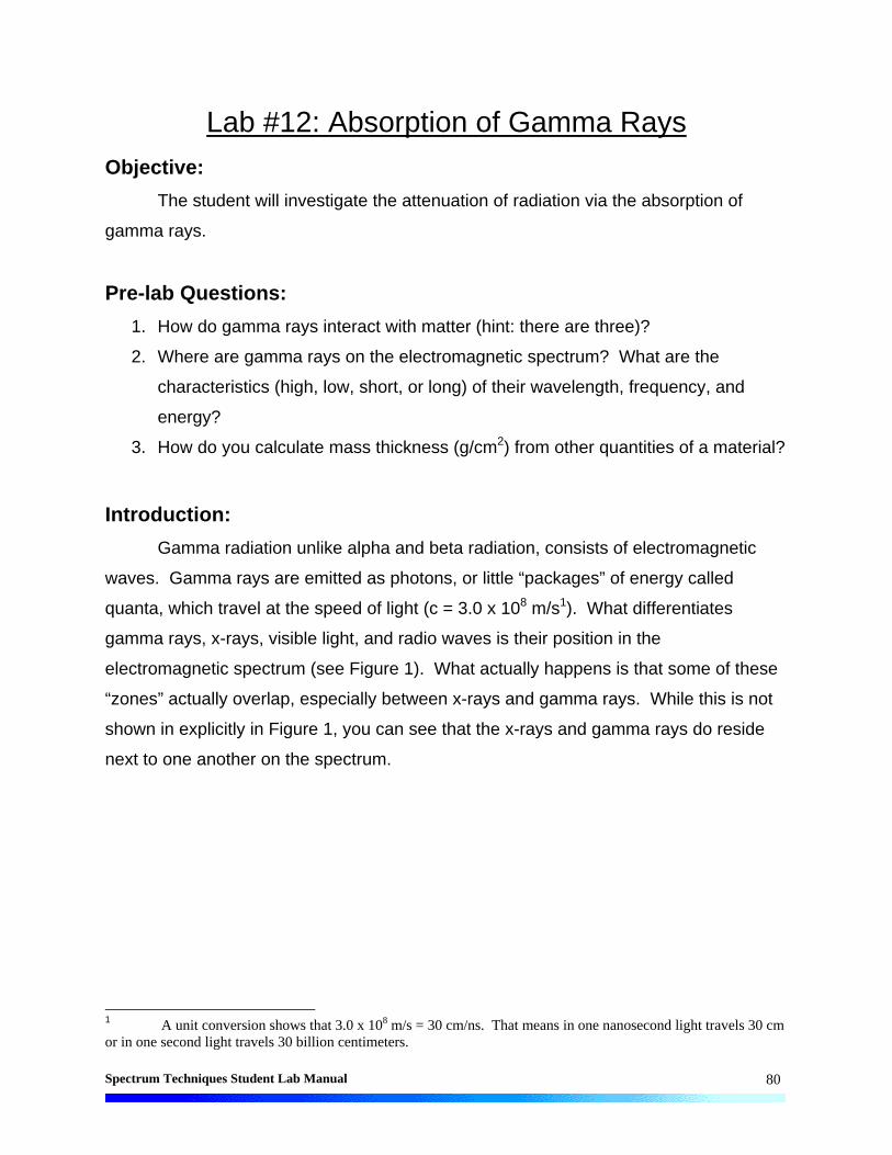
Spectrum Techniques Student Lab Manual
80
Lab #12: Absorption of Gamma Rays
Objective:
The student will investigate the attenuation of radiation via the absorption of
gamma rays.
Pre-lab Questions:
1. How do gamma rays interact with matter (hint: there are three)?
2. Where are gamma rays on the electromagnetic spectrum? What are the
characteristics (high, low, short, or long) of their wavelength, frequency, and
energy?
3. How do you calculate mass thickness (g/cm2) from other quantities of a material?
Introduction:
Gamma radiation unlike alpha and beta radiation, consists of electromagnetic
waves. Gamma rays are emitted as photons, or little “packages” of energy called
quanta, which travel at the speed of light (c = 3.0 x 10⁸ m/s1). What differentiates
gamma rays, x-rays, visible light, and radio waves is their position in the
electromagnetic spectrum (see Figure 1). What actually happens is that some of these
“zones” actually overlap, especially between x-rays and gamma rays. While this is not
shown in explicitly in Figure 1, you can see that the x-rays and gamma rays do reside
next to one another on the spectrum.
1 A unit conversion shows that 3.0 x 10⁸ m/s = 30 cm/ns. That means in one nanosecond light travels 30 cm or in one second light travels 30 billion centimeters.

Spectrum Techniques Student Lab Manual
81
Figure 1: The electromagnetic spectrum
One significant difference between x-rays and gamma rays is their origin. X-rays
are produced in the electron shells, while gamma rays are produced in the nucleus. X-
rays are created when electrons undergo a deceleration or jump to lower energy levels.
Gamma rays are created by energy transitions in the nucleus. In this experiment, we
are mostly concerned with gamma rays, because any x-rays present will be shielded by
air and matter acting as absorbers.
When a beam of gamma rays impinges on a sheet of absorbing material, some
of the radiation will be absorbed or scattered2. As the thickness of the absorber is
increased, the fraction of the radiation passing through will decrease. When exactly half
the radiation passes through the absorber (and the other half is absorbed or scattered),
the thickness of the absorber is called the half thickness, X1/2.
2 Gamma rays interact with matter in three ways: (1) photoelectric effect (ionization), (2) Compton effect, and (3) pair production (e+e-). Your instructor can explain more.
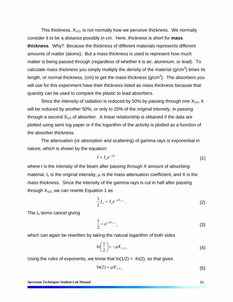
Spectrum Techniques Student Lab Manual
82
This thickness, X1/2, is not normally how we perceive thickness. We normally
consider it to be a distance possibly in cm. Here, thickness is short for mass
thickness. Why? Because the thickness of different materials represents different
amounts of matter (atoms). But a mass thickness is used to represent how much
matter is being passed through (regardless of whether it is air, aluminum, or lead). To
calculate mass thickness you simply multiply the density of the material (g/cm3) times its
length, or normal thickness, (cm) to get the mass thickness (g/cm2). The absorbers you
will use for this experiment have their thickness listed as mass thickness because that
quantity can be used to compare the plastic to lead absorbers.
Since the intensity of radiation is reduced by 50% by passing through one X1/2, it
will be reduced by another 50%, or only to 25% of the original intensity, in passing
through a second X1/2 of absorber. A linear relationship is obtained if the data are
plotted using semi log paper or if the logarithm of the activity is plotted as a function of
the absorber thickness.
The attenuation (or absorption and scattering) of gamma rays is exponential in
nature, which is shown by the equation:
XoeII (1)
where I is the intensity of the beam after passing through X amount of absorbing
material, Io is the original intensity, is the mass attenuation coefficient, and X is the
mass thickness. Since the intensity of the gamma rays is cut in half after passing
through X1/2, we can rewrite Equation 1 as
2/1
2
1 Xoo eII . (2)
The Io terms cancel giving
2/1
2
1 Xe , (3)
which can again be rewritten by taking the natural logarithm of both sides
2/12
1ln X
. (4)
Using the rules of exponents, we know that ln(1/2) = -ln(2), so that gives
2/1)2ln( X . (5)

Spectrum Techniques Student Lab Manual
83
One final rearrangement gives us a value of the mass attenuation coefficient
2/12/1
693.0)2ln(
XX . (6)
During your data analysis, you will find a value for X1/2, and thus one for .
Equipment:
Set-up for ST-360 Counter with GM Tube and stand (Counter box, power
supply – transformer, GM Tube, shelf stand, USB cable, and a source holder
for the stand) – shown in Figure 2.
Figure 2: Setup for ST360 with sources and absorber kit.
Radioactive Source (gamma ray emitter – any of the sources pictured in
Figure 3).
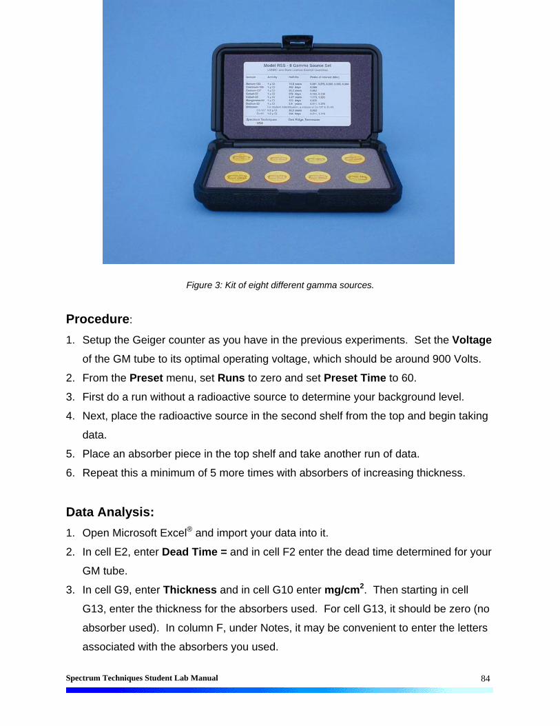
Spectrum Techniques Student Lab Manual
84
Figure 3: Kit of eight different gamma sources.
Procedure:
1. Setup the Geiger counter as you have in the previous experiments. Set the Voltage
of the GM tube to its optimal operating voltage, which should be around 900 Volts.
2. From the Preset menu, set Runs to zero and set Preset Time to 60.
3. First do a run without a radioactive source to determine your background level.
4. Next, place the radioactive source in the second shelf from the top and begin taking
data.
5. Place an absorber piece in the top shelf and take another run of data.
6. Repeat this a minimum of 5 more times with absorbers of increasing thickness.
Data Analysis:
1. Open Microsoft Excel® and import your data into it.
2. In cell E2, enter Dead Time = and in cell F2 enter the dead time determined for your
GM tube.
3. In cell G9, enter Thickness and in cell G10 enter mg/cm2. Then starting in cell
G13, enter the thickness for the absorbers used. For cell G13, it should be zero (no
absorber used). In column F, under Notes, it may be convenient to enter the letters
associated with the absorbers you used.

Spectrum Techniques Student Lab Manual
85
4. In cell H9 enter Dead Corr. and in cell H10 enter Counts. Then starting in cell H13,
enter a formula to correct for the dead time of the GM counter. Copy this formula
down the column for all the data you collected.
5. In cell I9 enter Corrected and in cell I10 enter Counts. Then starting in cell I13,
enter a formula to correct for the background of the GM counter. Copy this formula
down for all the data you have.
6. Next, make a graph of Corrected Counts per Minute vs. Thickness. Start with the
Chart Wizard either by choosing Chart from the Insert Menu or pressing its icon on
the top toolbar.
7. Select the Thickness values in the G column and the Corrected Counts values in
the I column.
8. Fill in the Chart Title, Value (X) Axis, and Value (Y) Axis windows with appropriate
names and units (if applicable) for those items.
9. Choose whether you want to view your graph as a separate worksheet as your data,
or you wish to see a smaller version of the graph with the data.
10. Right click on the y-axis of the graph and choose the Format Axis option. Then
choose the Scale Tab, and check the Logarithmic Scale option towards the
bottom.
11. Add a trendline to your data to obtain the equation of the best fit line through your
data.
Conclusions:
From your best-fit line equation, find the values for X1/2 and . Make sure your
answers are in the appropriate units (involving grams and centimeters).
Post-Lab Questions:
1. Is your data linear? If not, why?
2. Looking at your data and equating intensity and counts per minute, does your
result for X1/2 a correct approximation? (Does your result match the data?)
3. Can we be completely shielded from gamma rays? If not, then why bother?

Spectrum Techniques Student Lab Manual
86
4. Comparing your range for alpha particles, the absorption of beta particles,
and now the results for gamma rays, why are they different?

Spectrum Techniques Student Lab Manual
87
Data Sheet for Gamma Absorption Lab
Tube #: Run Duration:
Dead Time: (Time)
Counts Corr. Counts Thickness ln (Counts)
Equation for line: y=
mg/cm^2
OR g/cm^2
Calculate x_1/2 = ln(2)/
x_1/2 = g/cm^2
Name: Lab Session: Date: Partner:
Don’t forget to hand in a graph of the data with this table.

Spectrum Techniques Student Lab Manual
88
Lab #13: Half-Life of Ba-137m
Objective:
The student will measure the half-life of metastable Barium-137.
Pre-lab Questions:
1. Explain how you will obtain Ba-137m from the isotope generator.
2. Draw the decay diagram for the process you describe in #1.
3. If a Sr-90 source has a count rate of 7020 cpm today, when will it have a count rate
of 1404 cpm? The half-life of Sr-90 is 28.6 yrs. When will Po-210 reach 1404 cpm
from 7020 cpm (half-life for Po-210 is 138 days)?
4. If a Tl-204 source has 1.34 x 10²¹ atoms today. When will it have 1.675 x 10¹⁸
atoms? The half-life for Tl-204 is 3.78 years.
Introduction:
The decay of radioactive atoms occurs at a constant rate. There is no way to
slow it down by maybe refrigeration or to accelerate the process with heat. The rate of
decay is also a constant, fixed rate regardless of the amount of radioactive atoms
present. That is because there are only two choices for each atom, decay or don’t
decay. Thus, the amount of radioactive atoms we have on hand at any time is
undergoing a consistent, continuous change.
The change in the number of radioactive atoms is a very orderly process. If we
know the number of atoms present and their decay constant (probability of decay per
unit time), then we can calculate how many atoms will remain at any future time. This
can be written as the equation
tNNtN )( , (1)
where N(t) is the number of atoms that will be present at time t, N is the number of
atoms present currently, is the decay constant, and t is the elapsed time. If the
number of radioactive atoms remaining is plotted against time, curves like those in
Figure 1 can be obtained. The decay constant can be obtained from the slope of these
curves (discussed more below).

Spectrum Techniques Student Lab Manual
89
Figure 1: Exponential and Linear decay curves shown respectively
A more common way of expressing the decay of radioactive atoms is the half-
life. The half-life of a radioactive isotope is the time required for the disintegration of
one-half of the atoms in the original sample. In the graphs in Figure 1, 1000 atoms
were present at t = 0. At the end of one half-life, 500 atoms were present. At the end of
two half-lives, 250 atoms were present, one-quarter of the original sample. This
continues on and on, and example of what happens in the first nine half-lives is shown
in Table 1.
# of Half-lives Activity Percent Fraction 0 1000 100% 1 1 500 50% 1/2 2 250 25% 1/4 3 125 12.5% 1/8 4 62.5 6.25% 1/16 5 31.25 3.125% 1/32 6 15.625 1.563% 1/64 7 7.8125 0.781% 1/128 8 3.90625 0.391% 1/256 9 1.953125 0.195% 1/512
Table 1: Table of Example of Radioactive Decay
Since the observed activity of a sample as detected by a Geiger counter is
proportional to the number of radioactive atoms, it is not necessary to know exactly how
many atoms are present to determine either the half-life or the decay constant. Any
quantity of sample providing a suitable activity may be used. The derivations presented
below use the number of radioactive atoms but could very easily be substituted with
0
200
400
600
800
1000
1200
0 2 4 6 8 10
Number of Half-lives
Act
ivit
y
0
1
2
3
4
5
6
7
8
0 2 4 6 8 10
# of Half-lives
LN
of
Act
ivit
y

Spectrum Techniques Student Lab Manual
90
activity, since activitytime
atomsof
time
countsof ## . (Each count of a GM tube represents
one atom decaying and releasing one particle or ray of radiation.)
Looking back at Equation (1) in a slightly rearranged form
tNNtN )( . (2)
But N(t)-N is just the change in the number of radioactive isotopes of the original type
present, so we can define
tNNtNN )( . (3)
Dividing both sides of the equation gives
Nt
N
, (4)
but in calculus1 we write changes, especially small, or infinitesimal, changes as
Ndt
dN . (5)
This is a separable differential equation that becomes
dtN
dN , (6)
which can be solved by integrating both sides. When we do this we impose limits for
the integrals2, and pull out of the integral because it is a constant. The limits for dN’/N’
are from No to N, which is from the initial number of particles (No) to the new amount of
particles (N). The limits for dt are from the beginning, where t=0, to the end
tN
Ntd
N
dNo 0'
'
. (7)
The solution to this equation is
tNN o )ln()ln( . (8)
Solving for ln(N), gives
tNN o )ln()ln( . (9)
1 If you have not had Calculus yet, do not worry about the details of the derivation. Concentrate on the second part where natural logarithms are used. You should have this knowledge to perform the lab. 2 We have to change dN/N to dN'/N' because one of the limits is N, and we are not allowed to have a limit that is the same as the differential (dN part). For the same reason, we change dt to dt’. This is a basic substitution.

Spectrum Techniques Student Lab Manual
91
Thus, if we plot the natural log of the number of atoms (or activity) versus time, we will
get a straight line with slope = - and y-intercept = ln(No). This would allow us to find
the decay constant. Why?
We will need the decay constant in the next step, which is to find the half-life of
the radioactive isotope we are studying. Starting from Equation (8) and applying a
simple logarithmic identity, we get
tN
N
o
ln . (10)
If we are considering the half-life, then N is one-half of No (reduced ratio) and t is t1/2.
This changes our equation to be
2/12
1ln t
. (11)
Applying the reverse of our previous logarithmic identity, we get
2/1)2ln()1ln( t . (12)
The ln(1) = 0, so now we have
2/1)2ln( t . (13)
Finally, we can solve for the half-time
)2ln(
2/1 t . (14)
Equipment:
Set-up for ST-360 Counter with GM Tube and stand (Counter box, power
supply – transformer, GM Tube, shelf stand, USB cable, and a source holder
for the stand) – shown in Figure 2.
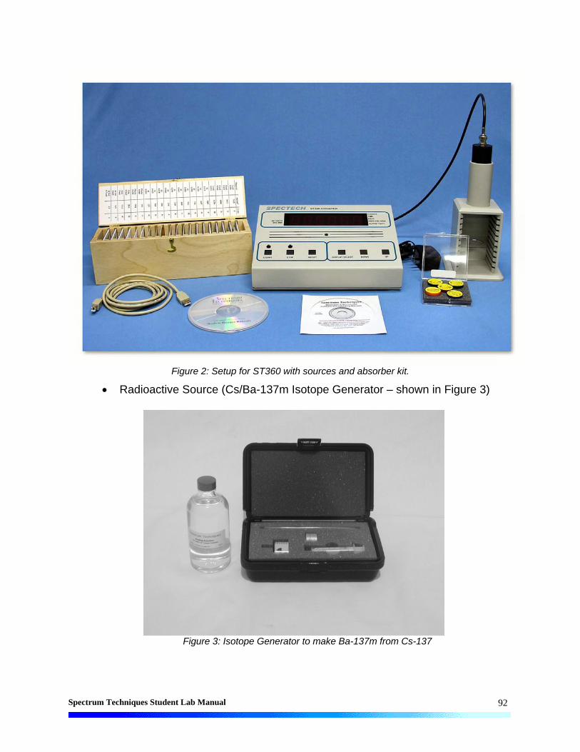
Spectrum Techniques Student Lab Manual
92
Figure 2: Setup for ST360 with sources and absorber kit.
Radioactive Source (Cs/Ba-137m Isotope Generator – shown in Figure 3)
Figure 3: Isotope Generator to make Ba-137m from Cs-137

Spectrum Techniques Student Lab Manual
93
Procedure:
1. Setup the Geiger counter as you have in the previous experiments. Set the Voltage
of the GM tube to its optimal operating voltage, which should be around 900 Volts.
2. From the Preset menu, set Runs to zero and set Preset Time to 30.
3. First do a run without a radioactive source to determine your background level.
4. Next, from the Preset menu, set the Runs to 31. (This will take 30 more runs so the
total number of runs is 31.)
5. From the isotope generator, obtain 10-12 drops of Ba-137m. Place the radioactive
source in the second shelf from the top and begin taking data.
6. Record the data to a file on disk or into a data table.
7. You may wish to do a second trial if time allows.
Data Analysis:
1. Open Microsoft Excel® and import your data into it.
2. In cell E2, enter Dead Time = and in cell F2 enter the dead time determined for your
GM tube.
3. In cell G9 enter Dead Corr. and in cell G10 enter Counts. In cell G13, enter a
formula to correct for resolving time and copy it down for the cells that have counts
in column C.
4. In cell H9 enter Corrected and in cell H10 enter Counts. In cell H13, enter a
formula to correct for background radiation and copy this down for the cells that have
counts in column G.
5. In cell I9 enter Natural Log and in cell I10 enter of Activity. In cell I13 and below,
enter a formula for the natural log (ln) of the corrected counts, and copy this down
for the cells that have counts in column H.
6. In cell J10 enter Time (s). In cell J13, enter 30. In cell J14, enter the formula
=J13+30, and copy this down for the cells that have entries in column I.
7. Next, make a graph of Natural Log (Ln) of Activity vs. Time. Start with the Chart
Wizard either by choosing Chart from the Insert Menu or pressing its icon on the top
toolbar.
8. Select Time values in the J column and the Ln of Activity values in the I column.

Spectrum Techniques Student Lab Manual
94
9. Fill in the Chart Title, Value (X) Axis, and Value (Y) Axis windows with appropriate
names and units (if applicable) for those items.
10. Adjust the size of the graph for your preference (or the instructor’s). You may also
wish to adjust the scales on one or more of the axes. Again, this is a preference
issue.
11. Right click on one of the data points and from the menu that appears, choose Add
Trendline. Make sure that the Linear option is chosen (should be darkened). Then
click on the Options tab and check the boxes for Display equation on chart and
Display R-squared value on chart. This will make the equation of the best-fit line
appear as well as a number that represents the percent of linearity of the data.
12. Make another graph, except this time use the Corrected Counts vs. Time. From this
graph, you will be able to see the true exponential nature of the decay and also be
able to estimate approximate half-lives.
13. Now, you will perform a linear regression over three different sets of numbers. A
linear regression finds the slope and y-intercept for the best-fit line through the data
chosen.
14. In the Tools menu, choose Data Analysis (ask your teacher if this option does not
appear). Then a small window will appear. Scroll down and choose the
Regression option. Now, a larger will appear. You will have to choose X-Values,
Y-Values, and an Output Range.
15. For the first linear regression, choose the first 15 data points under Natural Log of
Activity (column I) for the Y-Values by clicking on the box at the end of the input
window, outlining these numbers in column I, and then pressing the Enter key. (You
can either count 15 data points, or a small yellow box will appear and you enclose
numbers in the column until it reads 15R x 1C which means 15 rows in one column.)
Now, for the X-Values, choose the first 15 Time values in column J. Make sure the
Output Range is chosen. Then, either enter $M$1 in the input window or click on
the box and choose the M1 square. Click on OK and the results will appear on the
spreadsheet.

Spectrum Techniques Student Lab Manual
95
16. For the second linear regression, choose the data points 16-30 and choose the
output range to be M19. (We are squeezing them together because if you print in
landscape, these two will be on the same page.)
17. For the third linear regression, choose all 30 data points and choose the output
range to be M37. Does the slope for this linear regression match the slope from the
first graph?
18. To perform your final calculations, you will need the slopes from these linear
regressions and the error for the slope. The slope is the Coefficient of the X-
Variable (Why?) and is found in cells N18, N36, and N54. The error is the Standard
Error of the X-Variable and is found in cells O18, O36, and O54.
Conclusions:
Fill in the following table:
Data Points t1/2 Error # of ’s
First Half
Second Half
All
The variable is the decay coefficient. If you assumed you plotted Equation (9), then
the slope from the linear regression is the negative of
)(slope . (15)
From Equation (14), you can calculate the half-life:
693.0)2ln(
2/1 t . (16)
If you perform the proper error propagation, then you will end up with a final equation of
2/1
2/1
tt
. (17)
Rearranging this equation to calculate 2/1t gives
2/12/1
tt
. (18)

Spectrum Techniques Student Lab Manual
96
Now, to find the number of ’s that your result is away from the true value of t1/2 = 153 s,
we use the following equation
2/1
'#t
truemeasuredsof
. (19)
What you measure is the distance from your result to the true value and then see how
many standard deviations that is. The rule of thumb is that the result should be no
more than 2 ’s away from the true value to be statistically good.
Post-Lab Questions:
1. Write your result with the error, i.e. 153 s ± 1 s. Is this result (statistically)
good? (Recall that any value judgments must be justified.)
2. Which of the three results is better? Why?
3. How can the situation in #2 be resolved so that a linear regression over all the
data gives a more valid result? (How can you combine the halves of the
data?)

Spectrum Techniques Student Lab Manual
97
Data Sheet for Half-Life Lab
Tube #: Run Duration:
Dead Time: (Time)
Counts Corr. Counts ln(Counts) Time
(Background Count)
30
60
90
120
150
180
210
240
270
300
330
360
390
420
450
Name: Lab Session: Date: Partner:

Spectrum Techniques Student Lab Manual
98
Data Sheet for Half-Life Lab (Cont’d) Counts Corr. Counts ln(Counts) Time
480
510
540
570
600
630
660
690
720
Data t1/2 Error # of 's
First Half
Second Half
Whole
Don’t forget to hand in a graph of the data with this table.

Spectrum Techniques Student Lab Manual
99
Appendix A – SI Units The standard units of measure used in physics are the MKS (Meter, Kilogram, Second) version of the International System (SI) of Units. They are commonly referred to as the metric units. The latest version of the standards can be found in the following three resources: “Preferred Metric Units for General Use by the Federal Government,” (Federal
Standard 376B), January 27, 1993, General Services Administration. “Guide for the Use of International System of Units (SI),” (NIST Special Publication
811) (obtainable at the NIST website - http://www.nist.gov) “The International System of Units (SI),” (NIST Special Publication 330) (obtainable
at the NIST website – http://www.nist.gov)
Below, you will find the proper SI units – base and derived – that we will use. Also, there is a table showing the latest prefixes for SI Units.
Physical Quantity Name of Unit Symbol
Base Units
Length meter m Mass kilogram kg Time second t
Electric current ampere A Derived Units
Force newton N Energy joule J
electric potential volt V
electric resistance ohm electric capacitance farad F
activity (radioactive source) becquerel Bq
Table 1: Proper SI units that may be used in the lab manual.

Spectrum Techniques Student Lab Manual
100
Mulitplication Factor Prefix Name Prefix Symbol 1 000 000 000 000 000 000 000 000 = 1024 yotta Y 1 000 000 000 000 000 000 000 = 1021 zetta Z 1 000 000 000 000 000 000 = 1018 exa E 1 000 000 000 000 000 = 1015 peta P 1 000 000 000 000 = 1012 tera T 1 000 000 000 = 109 giga G 1 000 000 = 106 mega M 1 000 = 103 kilo k 100 = 102 hecto h 10 = 101 deca da 0.1 = 10-1 deci d 0.01 = 10-2 centi c 0.001 = 10-3 milli m 0.000 001 = 10-6 micro 0.000 000 001 = 10-9 nano n 0.000 000 000 001 = 10-12 pico p
0.000 000 000 000 001 = 10-15 femto f 0.000 000 000 000 000 001 = 10-18 atto a
0.000 000 000 000 000 000 001 = 10-21 zepto z 0.000 000 000 000 000 000 000 001 = 10-24 yocto y
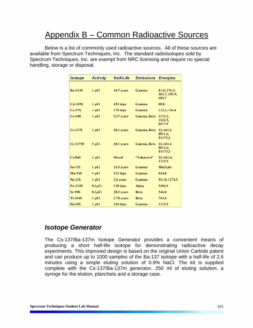
Spectrum Techniques Student Lab Manual
101
Appendix B – Common Radioactive Sources Below is a list of commonly used radioactive sources. All of these sources are available from Spectrum Techniques, Inc. The standard radioisotopes sold by Spectrum Techniques, Inc. are exempt from NRC licensing and require no special handling, storage or disposal.
Isotope Generator
The Cs-137/Ba-137m Isotope Generator provides a convenient means of producing a short half-life isotope for demonstrating radioactive decay experiments. This improved design is based on the original Union Carbide patent and can produce up to 1000 samples of the Ba-137 isotope with a half-life of 2.6 minutes using a simple eluting solution of 0.9% NaCl. The kit is supplied complete with the Cs-137/Ba-137m generator, 250 ml of eluting solution, a syringe for the elution, planchets and a storage case.

Spectrum Techniques Student Lab Manual
102
Appendix C – Statistics
Statistics play a very important part of physics, especially nuclear physics,
because we are dealing with atoms that number on the order of Avogadro’s number. It
is impossible to deal with every single atom individually, so we rely on statistics to give
us a prediction of behavior.
Statistics uses two main quantities in predicting behavior, the mean and the
standard deviation. The mean is the average, what most of the particles are doing.
The standard deviation tells us how many particles are also doing almost the same
thing as the mean. The previous experience that students usually have with mean and
standard deviation is from mathematics class (unless a statistics class has been taken).
From this experience, they know that mean can formulated by
N
i
i
N
xx
0, (1)
where x is the mean of a set of measurements ix (i = 1, 2, 3, …, N), and N is the
number of measurements taken.
Most students can recall how to calculate the standard deviation
1
0
2
N
xxN
ii
. (2)
What this equation does is measure the variance without regard to direction above or
below the mean (that is why you square and then square root – it is equivalent to
absolute value which just measures distance). These equations hold for most
everything the students have dealt with up to this point in school. The reason is that
most measurements follow a Gaussian distribution (symmetric about a mean).
Counting in nuclear physics is not symmetric about a mean. There is usually
some count rate that is pretty small because probability of decay is pretty small. Then
you also get high count rates. (Look back at the data from the statistics experiments
you performed this year.) When the data collects to a small number with a bit of a tail,
this is no longer a Gaussian distribution. The standard three statistical distributions will

Spectrum Techniques Student Lab Manual
103
be discussed below to assist the student learning more in detail about the statistics of
counting in nuclear physics. There are many more statistical distributions used for
various reasons but they will not be discussed here. (An example is the Landau
distribution used in describing the energy loss of a charged particle in matter, which is
different because it has an infinitely long tail to it.)
The first distribution is the Binomial distribution. This distribution is used when
you have two possible outcomes, the probability of getting one of those outcomes (and
thus the other) is a constant number independent of the number of trials, and the
selection of either outcome does not affect that outcome again in later trials. A good
example of this is flipping a coin.
To look at an example, we have an experiment where there are only two
outcomes A and B. In a binomial distribution, we deal with p, the probability that you will
get one of the outcomes (A), and q, the probability that the other outcome occurs (B).
Sometimes, instead of q, statistics books use 1-p, which is how q is calculated. Then,
the binomial distribution gives the probability, P(n), that n out of N objects are A is given
by
nNnnNn ppnnN
Nqp
nnN
NnP
1
!!
!
!!
!)( . (3)
Now for this distribution the mean, m, is given by
pNm (4)
and the standard deviation is calculated with any of the following
)1( pNpNpqmq . (5)
In order to study radioactive decays, we need a more useful distribution. We
need one for a very large number of counts and one that can handle a very small
probability of success (large N and small p). It just happens that the Poisson
distribution is the special case of the binomial distribution given those two conditions.
The Poisson distribution gives the probability, P(n), that n out of N objects are A as
mn
en
mnP
!)( , (6)
where m is the mean of the distribution (m = Np). The nicest feature of the Poisson
distribution is the ease to calculate standard deviation. The formula is

Spectrum Techniques Student Lab Manual
104
m . (7)
But for individual measurements, we take the standard deviation to be the square root
of the number of counts, here N,
N . (8)
So if you have a count rate of 10,000 cpm, then the standard deviation is ±100 cpm.
You may have noticed that for large values of m, the Poisson distribution
becomes hard to use. So we use a special case of the Poisson distribution for m>20
(the accepted rule of thumb), or a different special case of the Binomial distribution that
has large counts, low probability, and a large mean. This new distribution is called the
Normal or Gaussian distribution. This is the distribution that most students are familiar
with, its common name is the bell curve. Another added feature of this distribution is
that it can handle continuous variables (like most of those in our experiments), unlike
the Poisson and Binomial distributions, which can only handle discrete variables*. The
Gaussian distribution is given by
2
2
2exp
2
1)(
mx
nP . (9)
This equation gives us the mean and standard deviation equations that we are
accustomed to in Equations (1) and (2).
More details about statistical distributions must be researched in other books.
There is a huge amount of resources out there, statistical books and methods in
experimental physics books abound. There are some of the latter books listed below if
you wish to do more research. These should be available at most university libraries, or
through interlibrary loan services.
1. P.R. Bevington, D.K. Robinson, Data Reduction and Error Analysis for the Physical
Sciences, (McGraw-Hill, 1992).
2. G. Knoll, Radiation Detection and Measurement, (John Wiley & Sons, 1989)**.
3. N. Tsoulfanidis, Measurement and Detection of Radiation, (McGraw-Hill, 1995).
* The number of counts is a discrete, there is no such thing as a fraction of a count (there is nothing between 1 and 2). Length is a continuous variable, between 1 and 2 is 1.5. Between 1 and 1.5 is 1.25 and so on. * * There is a newer edition this one. This edition is the one the author owns.

Spectrum Techniques Student Lab Manual
105
4. W.R. Leo, Techniques for Nuclear and Particle Physics Experiments, (Springer-
Verlag, 1994)
Linear Regression
When Excel® or a graphing calculator performs a linear regression, it makes two
calculations to determine the slope and y-intercept of the best-fit line for the data. How
does it do it? Linear regressions are carried out using the method of least squares. This
method finds the line that minimizing the distance all the data points are away from the
best-fit line. This may sound complicated but it is really not if you know a little algebra
and one concept from calculus. Recall, that in math to find distance we use absolute
value, which is equivalent to the square root of the square*. (The squaring and
subsequent square rooting of a quantity is a common mathematical trick to substitute
taking an absolute value.) Let us start with an experiment, where you measure
variables x and y over N trials. The expected result is
y = mx + b
but remember that we take N measurements. So we get
y1 = mx1 + b
y2 = mx2 + b
….
yN = mxN + b.
These equations are not in general consistent; if we take different pairs of
equations, and solve them for m and b, we obtain different values for m and b. The
reason for the various values of m and b, of course, is that there are experimental errors
in the yi. Since the two sides of the equation, yi = mxi + b, are not exactly equal, but
differ by an amount let’s call d. To calculate d, we use
di = mxi + b – yi,
where di is the deviation corresponding to the ith equation and the pair of observations
(xi, yi). Since the values for di are the results of the experimental errors, we can assume
* The terms for absolute value and square root of a square are equivalent. That is
2xx .

Spectrum Techniques Student Lab Manual
106
that they are distributed according to the Gaussian (or normal) distribution. This allows
us to use the method of maximum likelihood to find the most probable values of m and
b.
This method finds the most probable values of m and b by minimizing the sum of
the squares of the deviations. That is, we minimize the quantity, d2, which has the form
i
iii ybmxd 22
.
The principle of least squares is finding the values of m and b that minimize d2. To
minimize the two variables, we take the partial derivative (due to the fact that m and b
are in the equation) of the function with respect to each of the variables (m and b) in
turn and set each derivative equal to zero. Rearranging the equations, we get 1
bNxmy ii and iiii xbxmyx 2,
where N is the number of points that are being used in the fitting process. Further
rearrangement, gives the following results for m and b:
22ii
iiyi
xxN
yxyxNm and
22
2
ii
iiiii
xxN
xyxxyb .
These values for m and b, are the slope and y-intercept, respectively, for the best-fit line
for the data. This is the calculation that a computer or calculator makes to output the
equation of the best-fit line.
Propagation of Errors
Often in laboratory experiments, the results will not be measured directly.
Rather, the results will be calculated from several measured physical quantities. Each
of these measured quantities consists of a mean (average) value and an error. What is
the resulting error in the final result of such an experiment? It is difficult to say how the
error of the measured quantities will translate (or propagate) to the error of the final
result.
The difficulty arises because we do not which sign, plus or minus, really exists for
the error. Recall that when reporting error, we show both signs, ±, to indicate that we
1 The summations, , are still over the index i but it has been dropped for convenience.

Spectrum Techniques Student Lab Manual
107
do not truly know where the true values lie. As an example, assume that we measure
two quantities, A ± A and B±B. (A and B represent the error on A and B,
respectively.) Then, we combine A and B into Z by Z = A + B. The extreme values of
the error are easy to predict, they are given by
BABABBAA or BABABBAA .
The problem is that most likely there is a mixture, some error from A cancels some of
the error or vice-versa. Then the situation becomes more complicated. However, this
problem has arisen before, the distance between two points on the Cartesian plane.
There we treat the distances independently (actually, perpendicular), but combine them
by the Pythagorean theorem. Simple enough solution, but what if the result, Z, depends
on both A and B (Z is a function of A and B). Then the problem uses the same method
but involves partial derivatives. (Note: The author considers this too complex of a
concept to explain here and refers any interested readers to their instruction or
multivariable calculus textbooks.) Due to the complexity of the work with partial
derivatives, the results of the error for various operations are given in the table below.
Operation Relation between Z, A, and B
Z = A + B 222 BAZ
Z = A – B 222 BAZ
Z = AB 222
B
B
A
A
Z
Z
Z = A/B 222
B
B
A
A
Z
Z
Z = nA *
A
An
Z
Z
Z = ln (A)
A
AZ
Z = eA
AZ
Z
* n is a constant (any real number)

Spectrum Techniques Student Lab Manual
108
Any further discussion of data analysis and error analysis techniques should be referred
to Taylor, John R. An Introduction to Error Analysis: The Study of Uncertainties in
Physical Measurements. University Science Books, 1982.

Spectrum Techniques Student Lab Manual
109
Appendix D - Radiation Passing Through Matter Our three forms of radiation must interact with matter while passing through it or
we would never be able to detect them. However, how they interact with matter is
completely different. Therefore, I will break this appendix up into three sections to study
alpha particles, beta particles, and gamma rays individually.
Alpha Particles
Alpha particles are helium nuclei, two protons and two neutrons, so it is
considered a heavy particle (compared to other particles in the universe). As an alpha
particle passes through matter, it passes close to many atoms. The positive charge
from the alpha particle attracts an electron from the valence shell of an atom it passes.
Sometimes the attraction is strong enough to free the electron from the atom, this
process is known as ionization. During this process, the alpha particle ends up giving
up some energy to the freed electron. This is the only true interaction that the alpha has
besides depositing its energy in some atoms through inelastic collisions. Either way,
the alpha particle loses some energy each time it interacts, which is denoted by
physicists as dE/dx. To calculate dE/dx, one uses the Bethe-Bloch formula which is
Z
C22
2ln
A
Z2 2
2max
22
2
222
I
WvmzcmrN
dx
dE eeea (1)
where 2 0 15352 2 2N r m c M eV cm ga e e . / and
re: classical electron radius = 2.817 x 10⁻¹³ cm me: electron mass = 9.11 x 10⁻³¹ kg
Na: Avogrado’s number = 6.022 x 10²³ / mol I: mean ionization energy
Z: atomic number of absorbing material A: atomic mass of absorbing material
: density of absorbing material z: charge of incident particle in units of e
= v/c of the incident particle = 1
1 2
: density correction C: shell correction
Wmax: maximum energy transfer in a single collision 22 cme .
Spectrum Techniques Student Lab Manual
110
Note that the equation for dE/dx is negative to indicate that it is an energy loss. There
are two correction terms, one for density effects and one for shell effects. While there
are many other possible corrections that could be made, they are negligible ( 1%).
The density effect arises due to the fact that atoms in the matter are polarized
by the electric field of the alpha particle passing through it. Thus, the electrons on the
far side of the atom will be shielded from interactions with the particle. However, the
denser the material, the closer the atoms are together and more shielding that occurs.
Since this term takes away possible interactions, is subtracted from the original formula.
The shell effect gives a small correction to the Bethe-Bloch formula, but still
must be taken into account. This effect only occurs when the velocity of the incident
particle is equal to or less than the orbital speed of the electrons. This situation
invalidates the assumption that the electrons are stationary with respect to the incident
particle.
While an alpha particle will lose energy in a collision, it is not much to make it
stray from its path. Therefore, an alpha particle passing through matter traverses it in a
relatively straight path while giving up energy in mainly ionization interactions.
Beta Particles
Beta particles are electrons that are emitted by the nucleus. They also undergo
the ionization energy loss as predicted by the Bethe-Bloch formula (Equation 1).
However, electrons are much less massive than alpha particles, m m 7342 , so there
is additional interaction due to the fact that the beta particle is greatly scattered through
matter. A beta particle passing close to a nucleus can have an electromagnetic
interaction that will slow the beta down and cause it to change directions; in essence it
will be braking. This “braking radiation” is described by its German name,
bremmstrahlung. Whenever the beta particle undergoes bremmstrahlung, it loses
energy but when an electron changes energy, it must absorb or emit electrons. Thus,
bremmstrahlung is the production of x-ray photons due to the interactions of electrons
(beta particles) with nuclei in matter.

Spectrum Techniques Student Lab Manual
111
Again, an alpha particle will pass almost straight through matter. The opposite is
true for a beta particle. It undergoes multiple scatterings that cause it path to be very
much of a “zigzag” pattern with no way to predict its path.
Gamma Rays
Gamma rays are photons that have an energy, frequency, and wavelength
sufficient enough to be classified as a gamma ray in the electromagnetic spectrum.
Photons interact three different ways in matter: (1) Photoelectric effect, (2) Compton
scattering, and (3) Pair production.
The photoelectric effect is when a photon is absorbed by an electron with the
subsequent ejection of the electron from the atom. The maximum energy of the ejected
electron is given by
KE Emax (2)
where E is the energy of the incident photon and is the work function (energy
necessary to free the electron).
Compton scattering is the scattering of photons on electrons. Originally, this
was only for free electrons but if the photon energy is sufficient to overcome the binding
energy, then we can consider the electron as free. In this collision, the photon is
incident on the electron with an energy h, where h is Planck’s constant and n is the
frequency of the photon. The photon undergoes an inelastic collision with the electron,
so the photon gives some of its energy to the electron. The photon leaves with a new
energy h’ and the electron leaves with a certain amount of kinetic energy that is E =
h-h’. We can calculate h’ by determining the scattering angle of the photon, . Then
we can use the equation:
cos11
hh (3)
The process of pair production refers to the transformation of a photon into an
electron-positron pair. In order to conserve momentum, this process can only occur
when the photon is close to the nucleus. Theoretically, the photon needs only the
energy that equates to the mass of an electron-positron pair. This energy is 1.022 MeV.
However, this process very, very rarely occurs below 1.5 MeV of photon energy,

Spectrum Techniques Student Lab Manual
112
because nature does not like creating the electron and positron and then having them
just sit there. Therefore, pair production only occurs when there is not only the mass
(energy) available, but also some extra energy for kinetic energy for the electron and
positron.
The photoelectric effect dominates for photon energies from 4 eV up to 0.5
MeV. Then Compton scattering dominates up to 2 MeV. Finally, pair production
dominates above 10 MeV, but only if a nucleus is present to absorb the momentum.
(Between 2 MeV and 10 MeV there is no true dominating absorption mechanism for
photons.)
For further reading on this topic, please refer to the Suggested References
section.

Spectrum Techniques Student Lab Manual
113
Appendix E – Suggested References
There is a large amount of information in books, journal articles, and on the Internet
relating to the topics in this lab manual (Radiation, particle interaction with matter, and
particle detection). Since many high school teachers do not have access to journals, I
have only listed books and website references.
Two of the best books on the topics of particle detectors that cover Geiger counters
are
Knoll, G. Radiation Detection and Measurement, John Wiley & Sons, 1989.
Tsoulfanidis, N. Measurement and Detection of Radiation, McGraw-Hill, 1995.
As for websites, there is a very large number of websites that would consume page
after page of this manual. Instead, this is a small sample of websites, which represent
the ones that the author deemed most helpful while writing this manual. They are not
listed in any particular order of importance, just alphabetically. Also, these sites were
verified in July of 2002, and any further accuracy of the information cannot be
guaranteed. In addition, if further resources are desired, do a search on a website such
as Google (http://www.google.com).
American Nuclear Society – http://www.ans.org This is the professional organization for nuclear engineers, nuclear scientists, and other nuclear related professionals. They sponsor very good programs for teachers in different areas of the country. There is large public information section covering many different levels of education.
EPA – Radiation Protection Program – http://www.epa.gov/radiation
This is the EPA’s webpage for how to protect the environment from radiation’s harm and explains how they clean it up after it happens. The EPA also tries to educate people that not all radiation is harmful.

Spectrum Techniques Student Lab Manual
114
Health Physics Society – http://www.hps.org
This is the professional organization for health physicists. It has more public information available, as well as an “Ask the Expert” area. Some of its regional chapters are excellent resources as well.
Nuclear Engineering 104A: Radiation Detection and Nuclear
Instrumentation Laboratory (Fall 2001) – http://www.nuc.berkeley.edu/dept/Courses/NE_104A
This link leads you to a list of files that comprise the course information. There is no main page that accesses all of the files. This course contains many materials on the basics of radiation and its detection.
RadEFX Radiation Health Effects Information Resource - http://radefx.bcm.tmc.edu/chernobyl
This is a very neat webpage where experts answer questions from basic radiation facts to questions mainly focusing on the worldwide effects of Chernobyl.
Radiological Information from the Collider-Acceleration Group at Brookhaven National Laboratory – http://www.agsrhichome.bnl.gov/AGS/Accel/SND/radiological_information.htm
This site covers radiation safety information from the most basic form to the very advanced concepts that are involved at the AGS and RHIC particle colliders at BNL. The link on elements is very good.
Texas Department of Health – Bureau of Radiation Control –
http://www.tdh.state.tx.us/ech/rad/pages/brc.htm
This is the website of the State’s controlling entity in Texas. (It is suggested that you find your state’s radiation department for information relevant to your state.) There may or may not be education information available, it depends on the state.

Spectrum Techniques Student Lab Manual
115
The Radiation and Health Physics Page – http://www.umich.edu/~radinfo/nojava.html
This is perhaps one of the best, or at least most referenced, webpage dealing with radiation on the Internet. It is a comprehensive website that does supply educational resources.
US Nuclear Regulatory Commission – http://www.nrc.gov
Find out what the controlling entity in the US for radiation does. There are also public information materials available.
University of Waterloo Radiation Safety Training – http://www.rstp.uwaterloo.ca
Good online training manual with a lot of basic information using animated gifs. Many of the particle interactions with matter are animated.
Uranium Information Centre (Melbourne, Australia) – http://www.uic.com.au/ral.htm
This is an awesome introduction to radiation all around us in everyday life. There are many good cartoon figures that explain the concepts being discussed.
Worcester Polytechnic Institute’s Radiation Safety Training and Reference Manual – http://www.wpi.edu/Admin/Safety/RSO/Training/trm.html
This radiation safety manual is online and covers the basics for many different professions that interact with radiation.

Spectrum Techniques Student Lab Manual
116
Appendix F – NRC Regulations
10 CFR 30.18, 30.71 Schedule B, and 32.19
§30.18 Exempt quantities. (a) Except as provided in paragraphs (c) and (d) of this section, any person is exempt from the requirements for a license set forth in section 81 of the Act and from the regulations in parts 30 through 34, 36 and 39 of this chapter to the extent that such person receives, possesses, uses, transfers, owns, or acquires byproduct material in individual quantities each of which does not exceed the applicable quantity set forth in §30.71, Schedule B. (b) Any person who possesses byproduct material received or acquired prior to September 25, 1971 under the general license then provided in §31.4 of this chapter is exempt from the requirements for a license set forth in section 81 of the Act and from the regulations in parts 30 through 34 of this chapter to the extent that such person possesses, uses, transfers, or owns such byproduct material. (c) This section does not authorize for purposes of commercial distribution the production, packaging, repackaging, or transfer of byproduct material or the incorporation of byproduct material into products intended for commercial distribution. (d) No person may, for purposes of commercial distribution, transfer byproduct material in the individual quantities set forth in §30.71 Schedule B, knowing or having reason to believe that such quantities of byproduct material will be transferred to persons exempt under this section or equivalent regulations of an Agreement State, except in accordance with a license issued under §32.18 of this chapter, which license states that the byproduct material may be transferred by the licensee to persons exempt under this section or the equivalent regulations of an Agreement State. [35 FR 6427, Apr. 22, 1970, as amended at 36 FR 16898, Aug. 26, 1971; 43 FR 6921, Feb. 17, 1978; 52 FR 8241, Mar. 17, 1987; 58 FR 7736, Feb. 9, 1993] §30.71 Schedule B.

Spectrum Techniques Student Lab Manual
117
Byproduct material Microcuries
Antimony 122 (Sb 122) 100 Antimony 124 (Sb 124) 10 Antimony 125 (Sb 125) 10
Arsenic 73 (As 73) 100 Arsenic 74 (As 74) 10 Arsenic 76 (As 76) 10 Arsenic 77 (as 77) 100
Barium 131 (Ba 131) 10 Barium 133 (Ba 133) 10 Barium 140 (Ba 140) 10 Bismuth 210 (Bi 210) 1 Bromine 82 (Br 82) 10
Cadmium 109 (Cd 109) 10 Cadmium 115m (Cd 115m) 10
Cadmium 115 (Cd 115) 100 Calcium 45 (Ca 45) 10 Calcium 47 (Ca 47) 10
Carbon 14 © 14) 100 Cerium 141 (Ce 141) 100 Cerium 143 (Ce 143) 100 Cerium 144 (Ce 144) 1 Cesium 131 (Cs 131) 1,000
Cesium 134m (Cs 134m) 100 Cesium 134 (Cs 134) 1 Cesium 135 (Cs 135) 10 Cesium 136 (Cs 136) 10 Cesium 137 (Cs 137) 10 Chlorine 36 (Cl 36) 10 Chlorine 38 (Cl 38) 10
Chromium 51 (Cr 51) 1,000 Cobalt 58m (Co 58m) 10
Cobalt 58 (Co 58) 10 Cobalt 60 (Co 60) 1 Cobalt 64 (Cu 64) 100
Dysprosium 165 (Dy 165) 10 Dysprosium 166 (Dy 166) 100
Erbium 169 (Er 169) 100 Erbium 171 (Er 171) 100
Europium 152 9.2 h (Eu 152 9.2 h)
100
Europium 152 13 yr (Eu 152 13 yr)
1
Europium 154 (Eu 154) 1 Europium 155 (Eu 155) 10
Fluorine 18 (F 18) 1,000 Gadolinium 153 (Gd 153) 10 Gadolinium 159 (Gd 159) 100
Gallium 72 (Ga 72) 10 Germanium 71 (Ga 71) 100
Gold 198 (Au 198) 100 Gold 199 (Au 199) 100
Hafnium 181 (Hf 181) 10 Holmium 166 (Ho 166) 100
Hydrogen 3 (H3) 1,000 Indium 113m (In 113m) 100 Indium 114m (In 114m) 10 Indium 115m (In 115m) 100
Indium 115 (In 115) 10 Iodine 125 (I 125) 1 Iodine 126 (I 126) 1 Iodine 129 (I 129) 0,1 Iodine 131 (I 131) 1 Iodine 132 (I 132) 10 Iodine 133 (I 133) 1 Iodine 134 (I 134) 10 Iodine 135 (I 135) 10
Iridium 192 (Ir 192) 10 Iridium 194 (Ir 194) 100
Iron 55 (Fe 55) 100 Iron 59 (Fe 59) 10
Krypton 85 (Kr 85) 100 Krypton 87 (Kr 87) 10
Lanthanum 140 (La 140) 10 Lutetium 177 (Lu 177) 100 Manganese 52 (Mn 52) 10 Manganese 54 (Mn 54) 10 Manganese 56 (Mn 56) 10
Mercury 197m (Hg 197m) 100 Mercury 197 (Hg 197) 100 Mercury 203 (Hg 203) 10
Molbdenum 99 (Mo 99) 100 Neodymium 147 (Nd 147) 100 Neodymium 149 (Nd 149) 100
Nickel 59 (Ni 59) 100 Nickel 63 (Ni 63) 10 Nickel 65 (Ni 65) 100
Niobium 93m (Nb 93m) 10 Niobium 95 (Nb 95)` 10 Niobium 97 (Nb 97) 10

Spectrum Techniques Student Lab Manual
118
Osmium 185 (Os 185) 10 Osmium 191m (Os 191) 100 Osmium 191 (Os 191) 100 Osmium 193 (Os 193) 100
Palladium 103 (Pd 103) 100 Palladium 109 (Pd 109) 100 Phosphorus 32 (P 32) 10 Platinum 191 (Pt 191) 100
Platinum 193m (Pt 193m) 100 Platinum 193 (Pt 193) 100
Platinum 197m (Pt 197m) 100 Platinum 197 (Pt 197) 100 Polonium 210 (Po 210) 0.1
Potassium 42 (K 42) 10 Praseodymium 142 (Pr 142) 100 Praseodymium 143 (Pr 143) 100 Promethium 147 (Pm 147) 10 Promethium 149 (Pm 149) 10
Rhenium 186 (Re 186) 100 Rhenium 188 (Re 188) 100
Rhodium 103m (Rh 103m) 100 Rhodium 105 (Rh 105) 100
Rubidium 86 (R86) 10 Rubidium 87 (Rb87) 10
Ruthenium 97 (Ru 97) 100 Ruthenium 103 (Ru 103) 10 Ruthenium 105 (Ru 105) 10 Ruthenium 106 (Ru 106) 1 Samarium 151 (Sm 151) 10 Samarium 153 (Sm 153) 100
Scandium 46 (Sc 46) 10 Scandium 47 (Sc 47) 100 Scandium 48 (Sc 48) 10 Selenium 75 (Se 75) 10
Silicon 31 (Si 31) 100 Silver 105 (Ag 105) 10
Silver 110m (Ag 110m) 1 Silver 111 (Ag 111) 100 Soldium 24 (Na 24) 10 Strontium 85 (Sr 85) 10 Strontium 89 (Sr 89) 1 Strontium 90 (Sr 90) 0.1 Strontium 91 (Sr 91) 10 Strontium 92 (Sr 92) 10
Sulphur 35 (S 35) 100 Tantalum 182 (Ta 182) 10 Technetium 96 (Tc 96) 10
Technetium 97m (Tc 97m) 100 Technetium 97 (Tc 97) 100
Technetium 99m (Tc 99m) 100 Technetium 99 (Tc 99) 10
Tellurium 125 m (Te 125 m) 10 Tellurium 127m (Te 127m) 10
Tellurium 127 (Te 127) 100 Tellurium 129m (Te 129m) 10
Tellurium 129 (Te 129) 100 Tellurium 131m (Te 131m) 10
Tellurium 132 (Te 132) 10 Terbium 160 (Tb 160) 10 Thallium 200 (Tl 200) 100 Thallium 201 (Tl 201) 100 Thallium 202 (Tl 202) 100 Thallium 204 (Tl 204) 10 Thulium 170 (Tm 170) 10 Thulium 171 (Tm 171) 10
Tin 113 (Sn 113) 10 Tin 125 (Sn 125) 10
Tungsten 181 (W 181) 10 Tungsten 185 (W 185) 10 Tungsten 187 (W 187) 100 Vanadium 48 (V 48) 10
Xenon 131m (Xe 131m) 1,000 Xenon 133 (Xe 133) 100 Xenon 135 (Xe 135) 100
Ytterbium 175 (Yb 175) 100 Yttrium 90 (Y 90) 10 Yttrium 91 (Y91) 10 Yttrium 92 (Y92) 100 Yttrium 93 (Y93) 100 Zinc 65 (Zn 65) 10
Zinc 69m (Zn 69m) 100 Zinc 69 (Zn 69) 1,000
Zirconium 93 (Zr 93) 10 Zirconium 95 (Zr 95) 10 Zirconium 97 (Zr 97) 10
Any byproduct material not listed above other than alpha emitting byproduct materials
0.1

Spectrum Techniques Student Lab Manual
119
§32.19 Same: Conditions of licenses. Each license issued under §32.18 is subject to the following conditions: (a) No more than 10 exempt quantities set forth in §30.71, Schedule B of this chapter shall be sold or transferred in any single transaction. For purposes of this requirement, an individual exempt quantity may be composed of fractional parts of one or more of the exempt quantities in §30.71, Schedule B of this chapter, provided that the sum of such fractions shall not exceed unity. (b) Each quantity of byproduct material set forth in §30.71, Schedule B of this chapter shall be separately and individually packaged. No more than 10 such packaged exempt quantities shall be contained in any outer package for transfer to persons exempt pursuant to §30.18 of this chapter. The outer package shall be such that the dose rate at the external surface of the package does not exceed 0.5 millirems per hour. (c) The immediate container of each quantity or separately packaged fractional quantity of byproduct material shall bear a durable, legible label which (1) identifies the radioisotope and the quantity of radioactivity, and (2) bears the words "Radioactive Material." (d) In addition to the labeling information required by paragraph (c) of this section, the label affixed to the immediate container, or an accompanying brochure, shall also (1) state that the contents are exempt from NRC or Agreement State licensing requirements; (2) bear the words "Radioactive Material -- Not for Human Use -- Introduction Into Foods, Beverages, Cosmetics, Drugs, or Medicinals, or Into Products Manufactured for Commercial Distribution is Prohibited -- Exempt Quantities Should Not be Combined"; and (3) set forth appropriate additional radiation safety precautions and instructions relating to the handling, use, storage, and disposal of the radioactive material. [35 FR 6428, Apr. 22, 1970]
Contact us: If we may be of help to you, feel free to contact us. Visit our web site for up-to-date information and products.
Spectrum Techniques, LLC
106 Union Valley Road
Oak Ridge, TN 37830 USA
Phone: 865-482-9937 FAX 865-483-0473
Email: [email protected]
Web site: www.SpectrumTechniques.com

N2 - 1 OPERATING CHARACTERISTICS OF THE GEIGER COUNTER
OBJECTIVE The objective of this laboratory is to determine the operating voltage for a Geiger tube and to calculate the effect of the dead time and recovery time of the tube on the counting rate. INTRODUCTION In medical and biological research, radioactive isotopes are utilized in three types of measurements: studies of the various chemical and physical interactions within a living organism or with its environment, measurements of the distribution of elements and compounds in the body and measurements of radioactive isotopes in the living organisms without taking samples. The techniques used in these measurements depend on the fact that the radioactive isotopes emit ionizing radiations, which can be detected by their effects on a photographic emulsion, or by electrical methods. Gases conduct electricity only when a number of their atoms are ionized, i.e. split up into a number of free electrons and positive ions. Alpha, beta or gamma radiation emitted by radioactive materials ionizes atoms with which they collide. Hans Geiger, an associate of Rutherford used this property to invent a sensitive detector for radiation.
Figure 1. The Geiger Counter
A "Geiger counter" usually contains a metal tube with a thin metal wire along its middle; the space in between them sealed off and filled with a suitable gas, and with the wire at a very high positive electric potential relative to the tube.
An electron, positive ion, or gamma radiation penetrating the tube through a mica window, will ionize a number of the atoms in the gas, and because of the high positive voltage of the central wire, the electrons will be attracted to it while the positive ions will be attracted to the wall. The high voltage will accelerate the positive and negative charges, they gain more energy and collide with more atoms to release more electrons and positive ions; the process escalates into an "avalanche" which produces an easily detectable pulse of current. With a suitable filling gas, the current quickly drops to zero so that a single voltage spike occurs across the resistor R and that is registered by an electronic counter. A typical composition of the gas filling in a Geiger
Outer Cylinder ( - Voltage)
Central Wire ( + Voltage)
R
V
Mica Window
+
_ Voltage spike to counter
α, β, or γ radiation

N2 - 2 counter tube was a mixture of argon and ethanol. More recently, tubes filled with ethyl formate in place of the alcohol are reported to have a longer life and smaller temperature coefficients than counters filled with ethanol. Very important is the self suppressing mechanism in a Geiger counter. The counter is triggered by the pulse from the tube and feeds back a square pulse of 300-500 µsec to the central wire. This pulse has an opposite polarity and high enough amplitude to extinguish the discharge.
The Geiger detector is usually called a "counter" because every particle passing through it produces an identical pulse, allowing particles to be counted; however, the detector cannot tell anything about the type of radiation or its energy/frequency (it can only tell that the radiation particles have sufficient energy to penetrate the counter. To improve sensitivity to alpha and beta particles, the ST150 detector has a very thin mica window with a superficial density of only 1.5 – 2 mg/cm2. This window is therefore extremely fragile and if broken cannot be repaired. Never allow any object to touch the window!
The Geiger Tube Voltage Characteristic
The most important information about a particular counter tube is the voltage characteristic curve. The counting rate due to a constant intensity radioactive source is graphed as a function of the voltage across the counter. A curve of the form shown in fig. 2 is obtained.
Figure 2: Geiger Tube Voltage Characteristic
The counter starts counting at a point corresponding approximately to the Geiger threshold voltage; from there follows a “plateau" with little change in the counting rate as the voltage increases. Finally a point is reached where the self-suppressing mechanism no longer works, and the counting rate rapidly increases until the counter breaks down into a continuous discharge. In order to ensure stable operation, the counter is operated at a voltage corresponding approximately to the mid-point of the plateau.
Counting Rate
Applied Voltage
Start Voltage
Geiger Threshold Voltage
Geiger Breakdown Voltage
Geiger Plateau
Operating Voltage V0
ProportionalDischarge Region
Continuous Discharge Region

N2 - 3 Hence a flat plateau is regarded as a desirable characteristic in a counter; a long plateau is also desirable, but not so important. In practice most counters have a slightly sloping plateau, partly because of geometrical limitations of the counter design, and partly because of spurious counts due to an unsatisfactory gas-filling or to undesirable properties of the cathode surface.
The correct operating voltage for the Geiger-Mueller tube will be determined experimentally using a small radioactive source such as Cs-137 or Co-60. A properly functioning tube will exhibit a "plateau" effect, where the counting rate remains nearly constant over a long range of applied voltage.
Resolving Time; Dead Time and Recovery Time. Geiger-Mueller tubes exhibit dead time effects due to the recombination time of the internal gas ions after the occurrence of an ionizing event. The actual dead time depends on several factors including the active volume and shape of the detector and can range from a few microseconds for miniature tubes, to over 1000 microseconds for large volume devices. The counter discharge occurs very close to the wire, and the negative particles, usually electrons, are collected very rapidly. The positive ions move relatively slowly, so that as the discharge proceeds a positively charged sheath forms around the wire. This has the effect of reducing' the field around the wire to a value below that corresponding to the threshold voltage, and the discharge ceases. The positive ion sheath then moves outwards until the critical radius r is reached, when the field at the wire is restored to the threshold value. This marks the end of the true "dead time". If another ionizing event triggers the counter at this stage, a pulse smaller than normal is obtained, as the full voltage across the counter is not operative. However, if the positive ions have reached the cathode before the next particle arrives, the pulse will be of full size. This effect can be demonstrated with a triggered oscilloscope, as shown in fig. 3, the period during which only partially developed pulses are formed being termed the "recovery time". The effective resolving time or insensitive time following a recorded pulse, is determined by both the dead time and the recovery time, and will depend not only on a number of parameters associated with the counter dimensions and gas filling, but in principle, also on the operating voltage of the counter, on the sensitivity of the electronic recording equipment and on the counting rate. It is necessary to apply appropriate corrections to observed counting rates to compensate for this resolving time.
Figure 3: Dead time and Recovery Time
Initial Geiger Discharge Counted
Second Geiger Discharge Counted
Possible Events Not Counted
Pulse Level
Time
Dead Time
Resolving Time = t
Recovery Time
Minimum Input Sensitivity Level of Counter
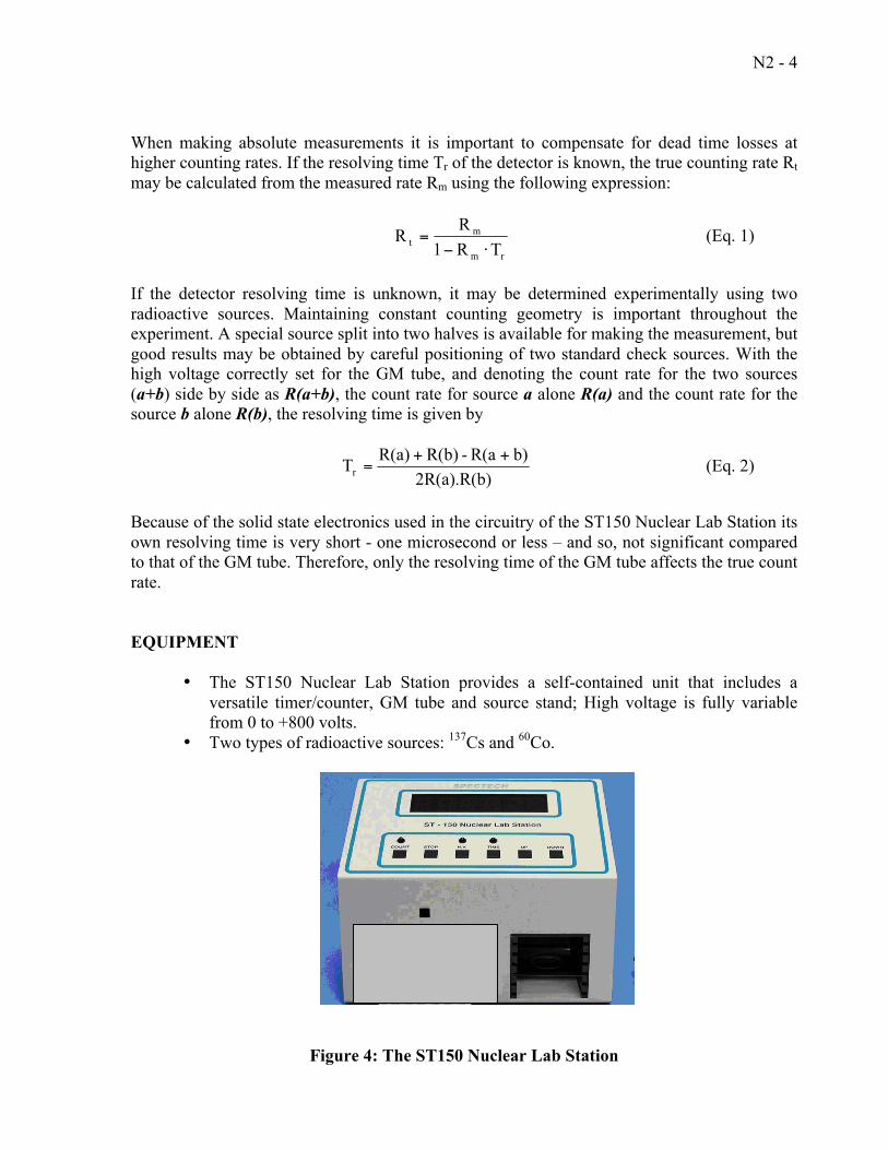
N2 - 4
When making absolute measurements it is important to compensate for dead time losses at higher counting rates. If the resolving time Tr of the detector is known, the true counting rate Rt may be calculated from the measured rate Rm using the following expression:
(Eq. 1)
If the detector resolving time is unknown, it may be determined experimentally using two radioactive sources. Maintaining constant counting geometry is important throughout the experiment. A special source split into two halves is available for making the measurement, but good results may be obtained by careful positioning of two standard check sources. With the high voltage correctly set for the GM tube, and denoting the count rate for the two sources (a+b) side by side as R(a+b), the count rate for source a alone R(a) and the count rate for the source b alone R(b), the resolving time is given by
(Eq. 2)
Because of the solid state electronics used in the circuitry of the ST150 Nuclear Lab Station its own resolving time is very short - one microsecond or less – and so, not significant compared to that of the GM tube. Therefore, only the resolving time of the GM tube affects the true count rate. EQUIPMENT
• The ST150 Nuclear Lab Station provides a self-contained unit that includes a versatile timer/counter, GM tube and source stand; High voltage is fully variable from 0 to +800 volts.
• Two types of radioactive sources: 137Cs and 60Co.
Figure 4: The ST150 Nuclear Lab Station

N2 - 5
PROCEDURE
PART I. GEIGER PLATEAU AND NORMAL OPERATING VOLTAGE
1. Sign out one radioactive source from your TA and place it on the transparent source stand close to the window of the GM detector.
2. Slowly increase the high voltage until radiation events just begin to be detected. 3. Now increase the voltage in 20 volt steps recording the counting rate at each increment.
The rate should remain fairly constant over a large range of voltage and then increase rapidly as the high voltage is further raised indicating that the tube is entering the breakdown region. Record your data in the table below.
4. Do not continue to operate the tube in this breakdown condition (you may irreversibly damage the tube); instead reduce the high voltage to zero.
Table 1: Data for Constructing a Plateau Curve
Run No Voltage (V) Counts Time (min) Counting Rate (Counts/min)
1.
2.
3.
4.
5.
6.
7.
8.
9.
10.
11.
12.
13.
14.

N2 - 6 DATA ANALYSIS
1. Using the data in table 1 make a plot of the counting rate versus the applied voltage. 2. The recommended Geiger operating voltage may be determined as the center of
the plateau region. In the example below the plateau extends from approximately 350V to 600V. A reasonable operating voltage in this case would be 500V.
Figure 3: Determination of Operating Voltage
(V)
N2 - 7 PART II. THE RECOVERY TIME OF THE TUBE
1. Set the high voltage to the operating voltage found in part I and the time interval for each count to 5 minutes.
2. Record all your data in the table below to calculate the recovery time t 3. Record the count rate for the first source (a) you have already used in part a as R(a). 4. Sign out a second radioactive source (b) from your TA and place both sources side by
side on the transparent source stand close to the window of the GM detector. 5. With the two sources (a+b) side by side, and the high voltage as the normal Geiger
operating voltage obtained in part I, record the count rate as R(a+b) for another 5 minutes.
6. Remove the first source (a), and return it to your TA 7. Record the count rate of the second source (b) as R(b).
Table 2: Data for Recovery Time
Voltage (V) Time (min) R(a) R(b) R(a+b)
DATA ANALYSIS
3. Using the recovery time find the adjusted true counting rates for the two sources using (Eq. 1).
4. Find the percentage difference between the measured and the true rates for both sources used.
5. Redraw the graph of counts vs. voltage in part one, using the adjusted true rates and determine the value of the normal operating voltage. How does the resolving time affect the value of this normal operating voltage determined in part I?

1
Experiment 4
Gamma Ray spectroscopy Using a Scintillation Detector
Objectives:
1. To learn the basic working principles and the components of a scintillation
detector.
2. To calibrate the scintillation detector system.
3. To observe the spectra of different gamma sources.
4. To find the resolution of the detector for different sources.
5. To study the full structure of 137Cs and 22Na spectra.
Theory:
1. Introduction to Scintillation detectors:
a. Description: The basic function of a scintillation detector, much like other types of detectors, is to transform the energy of an incoming particle to a measurable electronic signal. A scintillation detector consists of two components: 1. Scintillator.
2. Photomultiplier tubes (PMT).
The scintillator converts a fraction of the energy of the incoming particle to
light and the photomultiplier converts the light to a current signal, which
can be manipulated further in an electronics system.
• Scintillators:

2
A scintillator is a material that emits light, scintillates, when absorbing radiation. When a particle passes through the material it collides with atomic electrons, exciting them to higher energy levels. After a very short period of time the electrons fall back to their natural levels, causing emission of light. There are six different types of scintillators: 1. Organic crystals.
2. Organic liquids.
3. Inorganic crystals.
4. Plastics.
5. Gases.
6. Glasses.
In our experiment we will use Sodium Iodide (NaI ) crystal as our scintillator. NaI is an example of inorganic crystals. • Photomultiplier tubes (PMT): A photomultiplier is a device that converts photons to electric current. It consists of three parts: 1. Photocathode
2. Electron-Multiplier section (consisting of dynodes).
3. Anode.
In the photocathode an incident photon is absorbed by photoelectric effect,
releasing an electron. In the Electron-Multiplier section this electron is
accelerated through a series of secondary emission electrodes, dynodes,
knocking out a number of new electrons from each of them, multiplying the
number of electrons in each step. After multiplication, the total electron
current is collected in the anode.

3
Photomultiplier tube
b. Operation: In order to clarify how a scintillation detector operates; the system can be
divided into six consecutive stages involved in the detection of incident
radiation. These are:
SCINTILLATION DETECTOR ASSEMBLY DIAGRAM

4
1. Absorption of nuclear radiation in the scintillator.
2. The conversion of energy dissipated in the scintillator into emission of photons.
3. The transference of the light photons to the photocathode.
4. The absorption of the photons at the photocathode and the emission of the photoelectrons.
5. Electrons multiplication process within the photomultiplier.
6. The current pulse from the photomultiplier tube is amplified then analyzed by various electronic equipments.
c. Advantages:
1. It has high detection efficiency.
2. It has short dead time.
3. It has the ability to distinguish between types of radiations.
4. It can measure the energy of the radiation and hence can be used to identify different isotopes.
5. It has good energy resolution.
2. Calibrating the detector system:
The scintillation system gives the spectrum in terms of counts vs channel
numbers. A channel number is an integer that corresponds to the voltage
of the electron signal corresponding to each number of counts. Before we
can use the detector we need to convert these channel numbers into actual
energies. This process is called: energy calibration.
3. Energy resolution of a scintillation detector:
An important aspect of a Gamma ray spectrometer is the ability to distinguish between Gamma rays with slightly different energy. This quality is characterized by the so called energy resolution. The resolution at a certain energy peak in the spectrum is the ratio of some measure of the

5
width of the peak to the energy that corresponds to the center of the peak (the centroid). It is standard practice to use the Full-Energy Width at Half the Maximum peak count (FWHM) as the measure of the peak width. The energy resolution is then given by:
𝑅 = 𝐹𝑊𝐻𝑀
𝐸 × 100
Where: E is the energy of the centriod.
Gamma
spectrum from
the
decay of 137Cs.
4. Different structures in the gamma spectrum:
We will be mainly interested in 3 different structures each corresponding to
one of the ways by which gamma radiation interacts with matter. Namely
these ways are:
1. The photoelectric effect
2. Compton scattering
3. Pair production.
1. The Photopeaks:
These are peaks that correspond to the interaction of gamma rays by
the photoelectric effect. Here the incident photon disappears and a
photoelectron is produced with an energy that is very near to the
original energy of the incident photon. Hence these peaks are the most

6
important structures in the spectrum and the ones that are used to
identify different isotopes.
2. Compton edge:
This is due to Compton scattering by electrons. The Compton effect is an elastic “collision” of the gamma photon with an atomic electron in which relativistic mass-energy and momentum are conserved. After the collision, the electron has a kinetic energy that is a fraction of the gamma’s original energy, The gamma loses this energy, becoming a lower energy wave with
energy, E . The relation between the gamma’s energy before the collision compared to after the collision is
1
𝐸�́�−
1
𝐸𝛾=
1−cos 𝜃
𝑚𝑒𝑐2 (1)
Fig 1
where mec2 is the rest mass energy of the electron (511keV) and q is the angle through which the gamma is deflected. A depiction of the Compton scattering is shown in Figure 1. What is the origin of the Compton edge? A gamma enters the crystal of the detector and Compton scatters off an electron. The Compton-scattered gamma leaves the detector, so the amount of detected energy is the kinetic energy given to the electron. The maximum kinetic energy given to the electron, Emax, results from a “head-on” collision with the gamma, scattering the
gamma photon backwards ( = 180o). From equation (1) this maximum electron energy is:
𝐸𝑚𝑎𝑥 = 𝐸𝛾 − 𝐸�́� =2𝐸𝛾
2
2𝐸𝛾+𝑚𝑒𝑐2 (2)
This Emax is the energy of the Compton edge. Of course the electron may suffer a gentler collision and have less than the maximum energy after the collision. This is

7
the origin of the broad distribution of events at energies less than the Compton edge.
3. Annihilation peak:
When gamma rays that have energies higher than (1022 KeV) are incident
on the detector, some of the gammas can interact with the material
surrounding the detector crystal via pair production. The photon disappears
and an electron positron pair appears. The positron have a very short range
and hence it will combine with another electron shortly and the pair will
annihilate producing two gamma rays in opposite directions (to conserve
momentum) each of which has an energy of 511 keV. Since these photons
are in opposite directions only one will enter the detector. Those gammas
will cause a peak to appear in the spectrum at 511 KeV.
Apparatus:
Scintillation detector with (NaI) crystal.
MCA (multi channel analyzer) connected to computer.
Different Sources of gamma radiation.
Safety precautions: 1. Handle the radioactive sources with respect. Don’t bend or try to break them. 2. Never touch the source using bare hands. Always use forceps to handle sources. 3. Do not eat or drink during the lab. 4. Practice ALARA by being as far away from the sources as possible and returning the
source to your instructor as soon as you are finished with it and also by using appropriate shielding.
5. Lead is a potentially toxic material if it inters the body by swallowing or breathing its dust and if the exposure is long term. DO NOT touch your face or put your hands in your mouth after touching the lead bricks used for shielding. Always wash hands before leaving the lab.

8
Procedure:
1. Connect the detector to the computer (make sure not to confuse the HV cable with the NBC cable)
2. Connect the plugs to the electric mains and switch the computer and monitor ON.
3. Go to start menu then programs then spechtech and click on ICW16 to open the software.
4. Set the high voltage to 700 V and to the on position. (A green bar will appear on lower part of the window, written on it 700V indicating that the high voltage is on).
5. Put the Na22 source on the second shelf under the detector.
6. Click the start button (green diamond) on the software window to start counting and acquiring the spectrum. (see figure on next page)

9

10
7. After 10 minutes (when real time is at 600) click the stop button to stop
counting. Hover with the mouse over the rightmost peak in the Na22
spectrum and right click on it. Choose “ROI >>> set ROI” (region of interest)
and drag the pointer to shade the whole peak area. Write down the
centriod channel number.
8. Keep the spectrum and replace the Na22 source with a Ba133 source and
repeat steps 5-7 highlighting this time the rightmost peak of the Ba133
spectrum.
9. Calibrating the detector: On the menu bar go to: settings >>> energy
calibrate >>> two point calibrate. A window will pop up asking you which
units you want to use. Type: keV and click OK.
10. The following window will pop up.
Enter the channel number of the centroid of the Ba133 that you wrote
down in step 8 and enter the energy (356 keV) and click ok. Do the same for
cal point 2 entering the channel number of the centroid of the Na22 peak
and its known energy (1274.5keV). Click OK. Now your spectrum is
calibrated.
11. Go again to the ROIs that you shaded earlier and note for each the centriod
energy and the FWHM in table 1.
12. Set the other peak in the Na22 spectrum as a ROI and take its readings for
centroid and FWHM and write them down in table 1.

11
13. Click the erase button to erase the spectrum and right click anywhere in
the window. Choose : ROI >>> clear all.
14. Remove the Ba-133 source and put a Cs 137 source and acquire its
spectrum as you did with the previous two sources and the information of
the photopeak (centriod and FWHM) and write them in table 1.
15. Compton edge: For the same spectrum, calculate the Compton edge
energy. The Compton edge energy is the maximum energy (Emax) an
electron can get in a Compton scattering with a gamma photon. It is the
energy corresponding to about half the change in the count rate from the
trough between the photopeak and edge, to the immediate maximum in
the edge.
16. Remove the Cs-137 source and put a Co-60 source and acquire its spectrum
for 10 minutes and write down the centroids and FWHM for both peaks in
table 1.
17. Remove the Co-60 and put the unknown source and acquire its spectrum.
Write down the energies of the centroids of all its photopeaks.
18. Calculate the resolution of the detector for the various peaks of all the
sources you used.
19. From equation 2 find the rest mass of the electron and find the percentage
error in it.

12
Data sheet
Experiment 4: Gamma Ray spectroscopy Using a Scintillation
Detector
Sources information:
Data and calculations:
Calculating the energy resolution:
element Channel Number
Energy Centroid ( )
Energy FWHM ( )
R
22Na Peak 1
Peak 2
133Ba
137Cs
60Co Peak 1
Peak 2
Calculating the Compton edge energy (Emax) and the rest energy of the
electron.
- Counts corresponding to the trough between the photopeak and the
Compton edge: C1= ……………… (counts)
element activity (Ao) ( )
half-life t1/2
( ) Calibration date
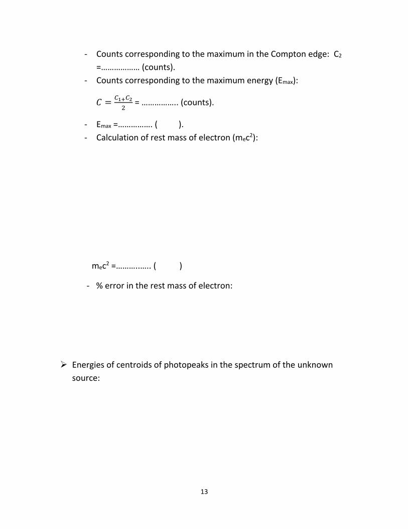
13
- Counts corresponding to the maximum in the Compton edge: C2
=……………… (counts).
- Counts corresponding to the maximum energy (Emax):
𝐶 =𝐶1+𝐶2
2 = …………….. (counts).
- Emax =……………. ( ).
- Calculation of rest mass of electron (mec2):
mec2 =………..….. ( )
- % error in the rest mass of electron:
Energies of centroids of photopeaks in the spectrum of the unknown
source:

14
Post lab questions:
1. For all the peaks in table 1 determine whether they are photopeaks
(resulting from photoelectric effect), Compton edges (resulting from
Compton scattering or pair annihilation peak. (You can check appendix E for
help if you need).
element Peak type
22Na Peak 1
Peak 2
133Ba
137Cs
60Co Peak 1
Peak 2
2. Use appendix E to determine the unknown isotope.
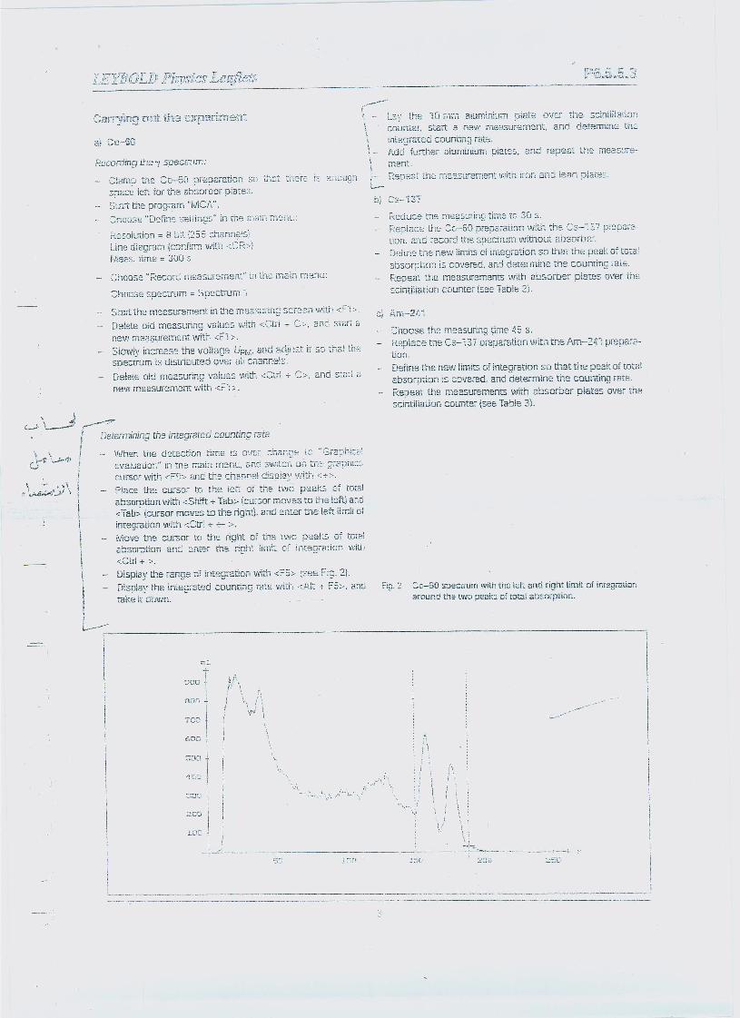

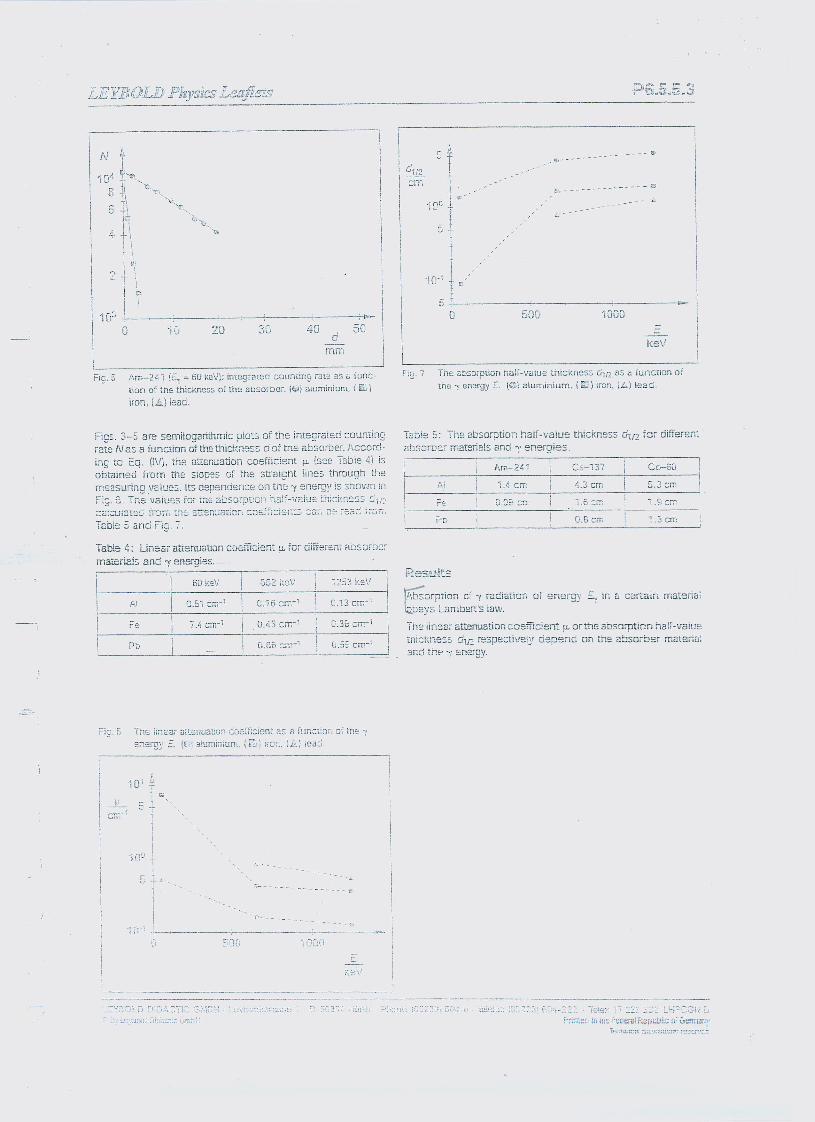

This section contains detailed information about unsealed
alpha emitting radiation sources. A radionuclide selection chart and plots of the alpha spectra are shown to help you to choose the right nuclide for your application.
ALPHA SPECTROMETRY
SOURCES
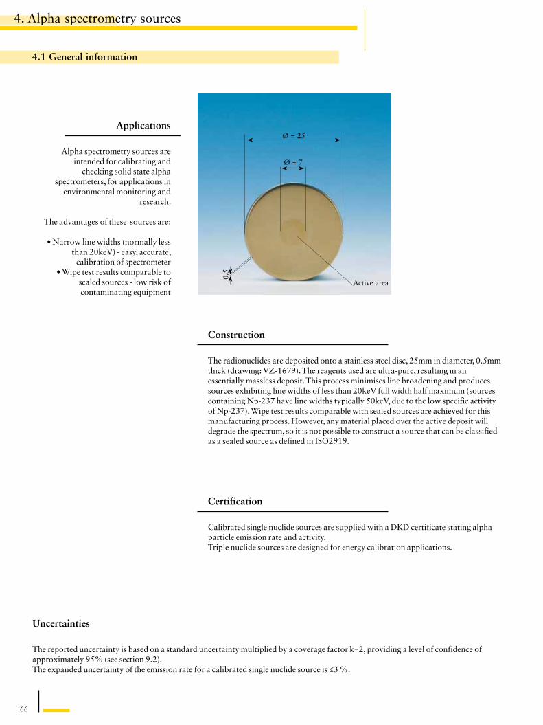
66
4. Alpha spectrometry sources
Applications
Alpha spectrometry sources are intended for calibrating and
checking solid state alpha spectrometers, for applications in
environmental monitoring and research.
The advantages of these sources are:
• Narrow line widths (normally less than 20keV) - easy, accurate,
calibration of spectrometer• Wipe test results comparable to
sealed sources - low risk of contaminating equipment
Ø = 25
Ø = 7
Active area
0.5
Construction
The radionuclides are deposited onto a stainless steel disc, 25mm in diameter, 0.5mm thick (drawing: VZ-1679). The reagents used are ultra-pure, resulting in an essentially massless deposit. This process minimises line broadening and produces sources exhibiting line widths of less than 20keV full width half maximum (sources containing Np-237 have line widths typically 50keV, due to the low specific activity of Np-237). Wipe test results comparable with sealed sources are achieved for this manufacturing process. However, any material placed over the active deposit will degrade the spectrum, so it is not possible to construct a source that can be classified as a sealed source as defined in ISO2919.
Certification
Calibrated single nuclide sources are supplied with a DKD certificate stating alpha particle emission rate and activity. Triple nuclide sources are designed for energy calibration applications.
Uncertainties
The reported uncertainty is based on a standard uncertainty multiplied by a coverage factor k=2, providing a level of confidence of approximately 95% (see section 9.2).The expanded uncertainty of the emission rate for a calibrated single nuclide source is ≤3 %.
4.1 General information

67
4.1 General Information
4. Alpha spectrometry sources
Traceability
The sources are traceable to standards held by national laboratories such as
the Physikalisch-Technische Bundesanstalt (Germany), the National Physical Laboratory (UK), the National
Institute of Standards and Technology (USA) the Laboratoire Primaire des
Rayonnements Ionisants (France), and many other national laboratories
world-wide. Further details are given in section 9.1.
Quality assurance
The sources are calibrated at Eckert & Ziegler Nuclitec GmbH’s
DKD accredited measurement laboratory in Germany. The
manufacturing facility operates a quality management system which has
been independently audited and approved to ISO9001:1994.
Recommendations on source handling
To maintain the accuracy of measurements, these sources must be handled with care. Sources should be handled with tweezers to avoid leaving grease on the surface of the source, which would degrade the spectrum. The sources must not be cleaned with abrasive compounds such as metal polish, as this would remove the active deposit. The sources should be kept in their storage boxes when not in use.
Tolerances
The maximum deviation of the measured activity at the reference time from the nominal value is +/-30%.
To help select the source needed, the energies and intensities of the most
intense alpha particles emitted by the different nuclides are shown in the
table.
Selection chart
Availability
The sources are normally delivered within 4-6 weeks from receipt of order.
Radionuclide Alpha particle energy [MeV] Intensity [%]
Np-237 4.640 6.2 4.766 8.0 4.772 25.0 4.788 47.0
Pu-239 5.105 11.5 5.143 15.1 5.155 73.4
Am-241 5.388 1.4 5.443 12.8 5.486 85.2
Pu-238 5.456 28.3 5.499 71.6
Cm-244 5.763 23.3 5.805 76.7

68
Cm-244CLRB2499 5.805 MeV
Pu-238PPRB2497 5.499 MeV
Am-241AMR23 5.486 MeV
Np-237
4.788 MeV
Pu-239PIRB2498
5.155 MeV
Pu-239
Am-241 Cm-244
Mixed nuclide sourceQCRB2500
4. Alpha spectrometry sources
Ordering information
1) For energy calibration only - no certificate of calibration is included2) For energy and efficiency calibration - certificate of calibration included3) The certificate of calibration states the total α emission rate and the nominal activities of
individual radionuclides
Radionuclide Nominal Energy of most intense Product code Product code activity alpha particle [MeV] uncalibrated 1) calibrated 2)
Am-241 50 Bq 5.486 AMR11 AMR21 Am-241 500 Bq 5.486 AMR12 AMR22 Am-241 5000 Bq 5.486 AMR13 AMR23 Am-241 40000 Bq 5.486 AMR14 not available
Pu-238 1000 Bq 5.499 PPRB2505 PPRB2497
Pu-239 1000 Bq 5.155 PIRB2506 PIRB2498
Cm-244 1000 Bq 5.805 CLRB2507 CLRB2499
mixed nuclide Pu-239 1000 Bq 5.155 QCRB2508 QCRB2500 3)
Am-241 1000 Bq 5.486 Cm-244 1000 Bq 5.805
mixed nuclide Np-237 150 Bq 4.788 QCRB4020 QCRB4021 3)
Am-241 100 Bq 5.486 Cm-244 100 Bq 5.805
4.2 Reference sources

69
4. Alpha spectrometry sources
Please photocopy the form on the next page, fill in the details as far as possible, and fax the form to your local Eckert & Ziegler Nuclitec GmbH office.
Alternatively, contact us by e-mail on:
or visit our internet page at:
http://www.nuclitec.de
We will reply via your local Eckert & Ziegler Nuclitec GmbH office.
4.3 Custom preparation service
If the alpha spectrometry source required is not shown in this catalogue, Eckert & Ziegler Nuclitec GmbH will try to assist you.

70
4. Alpha spectrometry sources
Nuclide(s) required :
Activity:
Dimensions of backing plate:
Any special requirement:
Date required by:
Our technical experts may be able to recommend an alternative source. If you wish, please tell us
your application:
EnquiryForm
Request for custom alpha spectrometry source
Your local Eckert & Ziegler Nuclitec GmbH office for forwarding the isotrak Technical Service
Name:
Institute/company
Address:
Country:
Tel:
Fax:
E-mail:
To:
From:
Date:

P6.5.6.1
© by LD DIDACTIC GmbH · Leyboldstrasse 1 · D-50354 Huerth · www.ld-didactic.com
Phone: +49-2233-604-0 · Fax: +49-2233-604-222 · E-mail: [email protected] · Technical alterations reserved
Atomic and nuclear physics Nuclear physics Compton effect
Quantitative observation of the Compton effect
Description from CASSY Lab 2 For loading examples and settings, please use the CASSY Lab 2 help.
CA
SS
Y L
ab 2
(2
01
2-0
9-2
7)

CASSY Lab 2
© by LD DIDACTIC GmbH · Leyboldstrasse 1 · D-50354 Huerth · www.ld-didactic.com
Phone: +49-2233-604-0 · Fax: +49-2233-604-222 · E-mail: [email protected] · Technical alterations reserved
333
Quantitative observation of the Compton effect
can also be carried out with Pocket-CASSY
Safety note
When handling radioactive preparations, in addition to the radiation protection regulations, state-specific require-ments and the regulations of the educational authorities are also to be observed, e.g. in the Federal Republic of Germany at the very least the radiation protection regulations (StrlSchV - Strahlenschutzverordnung) and the direc-tives on safety during school lessons. The preparation used in this experiment requires official permission! Before purchase, the radiation officer has to obtain permission from the authorities.
Since the used preparations produce ionizing radiation, the following safety rules must nevertheless be kept to:
· Prevent access to the preparations by unauthorized persons.
· Before using the reparations make sure that they are intact.
· For the purpose of shielding, keep the preparations in their safety container.
· To ensure minimum exposure time and minimum activity, take the preparations out of the safety container only as long as is necessary for carrying out the experiment.
· To ensure maximum distance, hold the preparations only at the upper end of the metal holder.
Experiment description
An energy calibration of the scintillation counter is made. The energy distribution of γ quanta scattered in an alumi-num scatterer is recorded for several angles between the source and the detector. From this the quantitative confir-mation of the Compton effect is obtained.
Equipment list
1 Sensor-CASSY 524 010 or 524 013 1 CASSY Lab 2 524 220 1 MCA box 524 058 1 Mixed preparation α, β, γ 559 845 or 559 835 1 Equipment set Compton 559 800 1 Cs-137 preparation, 3.7 MBq 559 809 (requires permission) 1 Scintillation counter 559 901 1 Detector output stage 559 912 1 High-voltage power supply 1.5 kV 521 68 1 PC with Windows XP/Vista/7

CASSY Lab 2
© by LD DIDACTIC GmbH · Leyboldstrasse 1 · D-50354 Huerth · www.ld-didactic.com
Phone: +49-2233-604-0 · Fax: +49-2233-604-222 · E-mail: [email protected] · Technical alterations reserved
334
Experiment setup (see drawing)
The output stage of the scintillation counter is connected to the MCA box and to the high-voltage power supply. The experiment panel from the Equipment set Compton is put down and the lead screening set up correspondingly.
Carrying out the experiment
Load settings
· First make an energy calibration of the scintillation counter. For this insert the mixed preparation in the sample holder from the Equipment set Compton, align it at the 0° mark. Leave the aluminum scatterer aside.
· Record the spectrum with , and make the energy calibration with the lines at 662 keV and 59.5 keV.
· Replace the mixed preparation with the Cs-137 preparation, set up the preparation at 30°, and set up the alumi-num scatterer. Place the additional screening in the direct line of vision between the preparation and the detector.
· Record the spectrum with , then remove the aluminum scatterer, and record a new spectrum.
· The difference between the two spectra (with and without the aluminum scatterer) is the scattering spectrum.
· Repeat the measurement at various angles of the preparation, each time subtracting a spectrum without the alu-minum scatterer from a spectrum with the aluminum scatterer. Always shift the additional screening in the setup so that the direct line of vision between the preparation and the detector is blocked.
Evaluation
From the scattering spectra (difference with and without aluminum scatterer) the energy of the scattered g quanta is determined. The values are plotted against the associated angles and compared with the theoretical values:
Alternatively a Free fit can be performed.


P6.5.3.1
LD Physics Leaflets
Atomic and Nuclear Physics Nuclear Physics Nuclear Magnetic Resonance
Nuclear magnetic resonance in polystyrene, glycerine and teflon
Objects g Nuclear Magnetic Resonance on protons and fluorine in liquids and solid samples g Determination of the line width of the fluorine resonance g Determination the g-factor of protons and fluorine
Principles Nuclear magnetic resonance (NMR) was discovered by Bloch and Purcell in 1945. NMR spectroscopy is nowadays an im-portant standard method in chemistry and biology. In medical applications NMR has established under the name Magnetic Resonance Imaging (MIR) as an imaging method for clinical diagnosis supplementary to scanning techniques involving x-ray and ultra sound. This experiment demonstrates the basic phenomenon of NMR on liquid and solid samples and gives first insight into spectroscopic applications in chemistry and biology. NMR is based on the magnetic properties of the nucleus. Atoms with a nucleus which possesses a nuclear spin I have a magnetic moment µn according the relation:
Ig n ⋅µ⋅−=µ (I)
µn: nuclear magneton g: g-factor
The nuclear magnets µ can orientate only in distinct direc-tions in respect to a static magnetic field B0. Each spin orien-tation corresponds to a particular energy level which is given by:
kBgE 0nk ⋅⋅µ⋅−= with k I,...,1I.I ++−−= (II)
When a sample is placed in a static magnetic field B0 the nuclear spins are distributed over the energy levels according the Boltzmann-equation:
LD Didactic GmbH . Leyboldstrasse 1 . D-50354 Hürth . Telefon: (02233) 604-0 . Fax: (02233) 604-222 . e-mail: [email protected]
Wie
110
5 )Tk
EEexp(
NN
B
k1k
1k
k −−= +
+ (III)
kB: Boltzmann constant Nk: Number of spins in level k
The spins may be excited to jump between adjacent energy levels Ek when the sample is exposed to a magnetic field B1 of high frequency ν which is perpendicular to the static field �0. Therefore the frequency ν have to match exactly the energy spacing. This is called resonance (∆k = 1):
0nk1k BgEEh ⋅µ⋅−=−=ν⋅ + (IV)
h: Planck’s constant In this experiment the NMR signals of Hydrogen nuclei (pro-tons) and fluorine nuclei are observed. Both nuclei have a spin of I = ½. and thus according to equation (II) they have only two possible orientations in respect to the magnetic field B0 (Fig. 1). In order to detect the spin transitions between these two energy levels the sample is placed in an rf coil which is located between the gap of a homogeneous field B0. Additionally, the static magnetic field B0 is modulated at con-stant frequency ν by the use two modulation coils. Thus in this setup the resonance signal is observed in dependence of the magnetic field. Each time when the resonance condition (i. e. equation IV) is fulfilled energy is absorbed from the rf coil due to the spin transitions. The NMR signal is propor-tional to the number of spins N in the sample. For example, an hydrogen nucleus the resonance frequency in a magnetic field is about 42.5 MHz. The precise value depends on the chemical environment of the hydrogen atom as in addition to the external magnetic field B0 the local inter-nal field of electrons and nuclei in the near vicinity also acts on the hydrogen nucleus. This is called chemical shift and makes NMR to an important spectroscopic method for chem-istry and biology.
LD Didactic GmbH Gedruckt in der Bundesrepublik Deutschland Technische Änderungen vorbehalten

P6.5.3.1 - 2 - LD Leaflets Physics
The line width of the NMR resonance line is influenced by the nature of the surrounding elements and on the temperature. The analysis of line width as function of these factors yields comprehensive information about chemical and physical characteristics of the various sample components. The full width of half maximum (Fig. 1) is under some circumstances a measure for the relaxation time T2:
2T1~~B ν∆∆ (V)
E(-1/2)
E(1/2)
B0
Ek
B
hν = ∆E
FWHM
E(-1/2)
E(1/2)
B0
Ek
B
hν = ∆E
FWHM
Fig. 1: Energy splitting of a nucleus of I = ½ in the magnetic field B0.
One line is observed in the NMR spectrum from which the full width at half maximum (FWHM) can be determined.
LD Didactic GmbH . Leyboldstrasse 1 . D-50354 Hürth . Telefon: (02233) 604-0 . Fax: (02233) 604-222 . e-mail: [email protected]
Setup - Mount the two coils on the U-core. - Slide the modulation coils onto the pole shoes and mount
the NMR-probe evenly on the U-core. - Connect the two coils in series with the DC power supply
according Fig. 2. - Connect the modulation coils in series with the “MODULA-
TION” output of the NMR supply unit. - Connect the NMR-probe to the input “PROBE” of the NMR
supply unit. - Connect the output “NMR SIGNAL” to the channel of verti-
cal deflection and the output “∆B SIGNAL” to the channel of horizontal deflection of the oscilloscope.
Fig. 2: Electrical setup of the NMR experiment, schematically. Apparatus
1 NMR-probe unit ..................................................514 606 1 NMR-supply unit.................................................514 602 1 U-core with yoke ................................................562 11 2 Coils, 10 A, 480 turns.........................................562 131 1 DC-power supply 0...16 V, 0...5 A ......................521 545 1 Analog Oscilloscope HM 303 .............................575211 2 BNC cables, 1m .................................................501 02 or 1 Sensor CASSY USB .....................................524010USB 1 CASSY Lab ........................................................524 200 2 Screen cables BNC/4mm...................................575 24 1 Safety Connection lead, 50 cm red ....................500 621 1 Safety Connection lead, 100 cm red ..................500 641 1 Safety Connection lead, 100 cm blue.................500 642
additionally recommended: 1 Universal Measuring Instrument Physics ...........531 835 1 Combi B-Sensor S .............................................5240381 1 Extension Cable, 15-pole ...................................501 11
Carrying out the experiment a) NMR on liquid and solid samples with protons - Set the oscilloscope to xy-mode - Select fast sweep and set the modulation amplitude to a
large value - Set the value of the frequency to a maximum value. - Slowly enhance the HF amplitude until the red LED lights
up and a frequency of about 19 MHz is displayed. - Reduce the frequency to a value of about 18.5 MHz. - Shift the O-ring of the glycerine sample tube (8 protons) so
that the sample will be located approximately in the center of the measuring chamber.
- Carefully insert the sample tube into the measuring cham-ber. Remark: if the sample tube is inserted at an angle with too much force the rf coil can be damaged.
- Slowly increase the current though the 10 A coils until an NMR signal appears on the oscilloscope of the screen.
LD Didactic GmbH Gedruckt in der Bundesrepublik Deutschland Technische Änderungen vorbehalten

LD Handblätter Physik - 3 - P6.5.3.1
- Optimize the NMR signal by slowly varying the HF ampli-tude.
- Shift the NMR signal to the center of oscilloscope screen by varying the magnet current or the frequency and adjust the modulation amplitude.
- Adjust the phase of the signal until the signal of up and down sweep coincide.
Remark: If you want to record the signals connect the appara-tus to the Sensor CASSY. - Repeat the experiment for a water sample, the polystyrene
sample and the polytetrafluorethylene sample.
b) NMR of solid a sample with fluorine nuclei - Repeat the experiment of part a) for the polytetrafluore-
thylene sample (PTFE). - Determine first how much a unit (e. g. from a major tick of
the x-axis to the other) on the oscilloscope screen of the horizontal deflection is in frequency units. This can be achieved by shifting the peak of NMR signal with the fre-quency button to a scale mark (e. g. tick of the x-axis) and note the frequency. Then shift the signal to the next scale mark and note again the frequency.
- Measure the line width at half maximum (FWHM) of the resonance line in units of the oscilloscope screen.
c) Application in Chemistry (NMR Spectroscopy) As an introduction to the application of NMR in chemistry the NMR signal of e. g. hand cream can be investigated. Hand cream naturally contains a lot of glycerine and depending on the type of hand cream also water. The spins of the hydrogen nuclei of the gycerine molecule can be detected by first optimizing the NMR apparatus with the glycerine sample according experiment part a) and then be compared with the signal of the hand cream. - Prepare a piece of a straw of about 50 mm of length an fill
it with hand cream (filling height approximately 10 mm to 15 mm).
- Clean the straw thoroughly, in particular, make sure that no hand cream is at the lower end of the straw to avoid pollution of the measuring chamber.
- Shift an O-ring over the straw so that the sample will be located approximately in the center of the measuring chamber.
- now optimize the NMR apparatus for the glycerine sample according experiment part a).
- Carefully remove the glycerine sample from the measuring chamber and insert the straw with the hand cream sample carefully.
- If necessary tune the frequency and observe the signal. Depending on the amount of sample it may be necessary to tune the frequency, too.
d) Application in Biology (Spectroscopy) As an introduction to the application of NMR in biology the NMR signal of e. g. an apple or plant can be investigated. Fruits like apples, green pepper etc. naturally contain water. The same holds for plants as for example flowers.
The spins of the hydrogen nuclei of the water molecule can be detected by first optimizing the NMR apparatus with the water sample according experiment part a) and then be com-pared with the signal of an apple or a plant. - Prepare a piece of a straw of about 50 mm of length an fill
it with the fruit flesh of an apple (filling height approxi-mately 10 mm to 15 mm).
- Clean the straw thoroughly, in particular, make sure that no apple pieces are at the lower end of the straw to avoid pollution of the measuring chamber.
- Shift an O-ring over the straw so that the sample will be located approximately in the center of the measuring chamber.
- now optimize the NMR apparatus for the water sample according experiment part a).
- Carefully remove the water sample from the measuring chamber and insert the straw with the apple sample care-fully.
- If necessary tune the frequency and observe the signal. Depending on the amount of sample it may be necessary to tune the frequency, too.
- Similarly, the NMR signal of protons in the stem of plants can be observed. Note, the stem should have a medium diameter.
e) Determination of the g-factor (Teslameter required) - Tune the NMR apparatus according to experiment part a)
for the glycerine sample at about 18 MHz and measure the frequency.
- Carefully remove the sample from the measuring chamber and measure the magnetic field with the Tangential B-Probe in the measuring chamber.
- Place the Tangential B-Probe according Fig. 3 at the pole shoes and measure the magnetic field.
TeslameterNMR Probe
Measuring chamber TeslameterNMR Probe
Measuring chamber
Fig. 3. Schematic depiction for placing the Tangential B-Probe
between the pole shoes of the magnet.
- Tune the NMR apparatus for the water sample at lower and higher frequencies by varying the current through the 10 A coils and measure the frequency and the magnetic flux density.
- Repeat the experiment for the polytetrafluorethylene (PTFE) sample.
LD Didactic GmbH . Leyboldstrasse 1 . D-50354 Hürth . Telefon: (02233) 604-0 . Fax: (02233) 604-222 . e-mail: [email protected] LD Didactic GmbH Gedruckt in der Bundesrepublik Deutschland Technische Änderungen vorbehalten
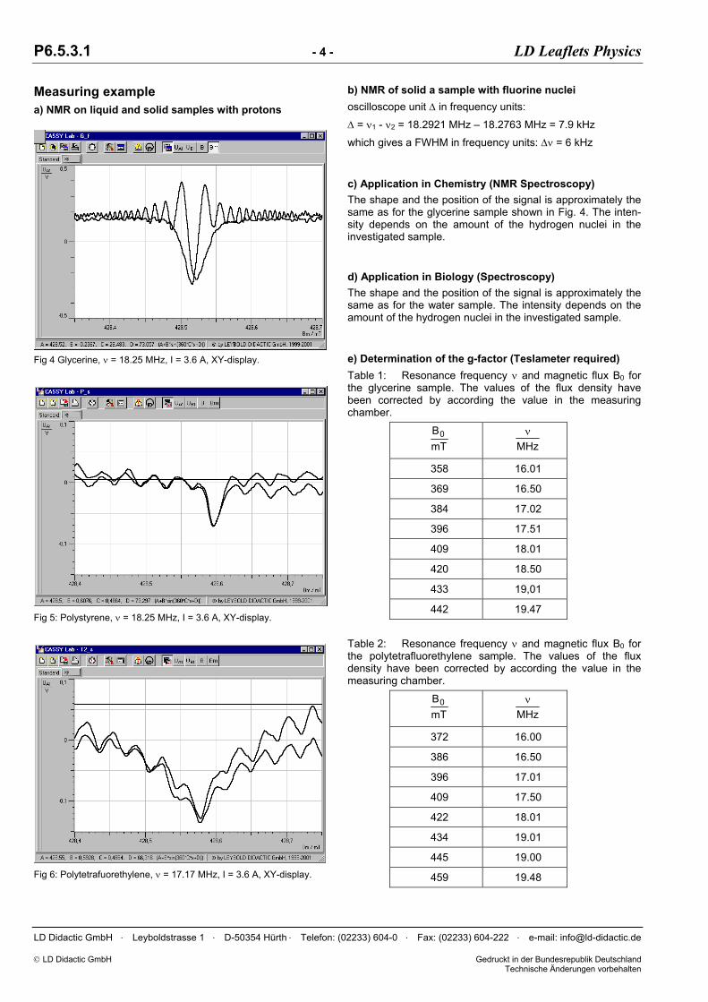
P6.5.3.1 - 4 - LD Leaflets Physics
Measuring example a) NMR on liquid and solid samples with protons
Fig 4 Glycerine, ν = 18.25 MHz, I = 3.6 A, XY-display.
LD Didactic GmbH . Leyboldstrasse 1 . D-50354 Hürth . Telefon: (02233) 604-0 . Fax: (02233) 604-222 . e-mail: [email protected]
Fig 5: Polystyrene, ν = 18.25 MHz, I = 3.6 A, XY-display.
Fig 6: Polytetrafuorethylene, ν = 17.17 MHz, I = 3.6 A, XY-display.
b) NMR of solid a sample with fluorine nuclei oscilloscope unit ∆ in frequency units:
∆ = ν1 - ν2 = 18.2921 MHz – 18.2763 MHz = 7.9 kHz
which gives a FWHM in frequency units: ∆ν = 6 kHz
c) Application in Chemistry (NMR Spectroscopy) The shape and the position of the signal is approximately the same as for the glycerine sample shown in Fig. 4. The inten-sity depends on the amount of the hydrogen nuclei in the investigated sample.
d) Application in Biology (Spectroscopy) The shape and the position of the signal is approximately the same as for the water sample. The intensity depends on the amount of the hydrogen nuclei in the investigated sample.
e) Determination of the g-factor (Teslameter required) Table 1: Resonance frequency ν and magnetic flux B0 for the glycerine sample. The values of the flux density have been corrected by according the value in the measuring chamber.
mTB0
MHzν
358 16.01
369 16.50
384 17.02
396 17.51
409 18.01
420 18.50
433 19,01
442 19.47
Table 2: Resonance frequency ν and magnetic flux B0 for the polytetrafluorethylene sample. The values of the flux density have been corrected by according the value in the measuring chamber.
mTB0
MHzν
372 16.00
386 16.50
396 17.01
409 17.50
422 18.01
434 19.01
445 19.00
459 19.48
LD Didactic GmbH Gedruckt in der Bundesrepublik Deutschland Technische Änderungen vorbehalten

LD Handblätter Physik - 5 - P6.5.3.1
Evaluation and results a) NMR on liquid and solid samples with protons If a sample contains hydrogen nuclei an NMR signal can be observed. The sample can be a liquid or a solid (powder) sample. However, due to the structure of the sample a signifi-cant difference in line width is observed for the NMR on Hy-drogen nuclei, e. g. the glycerine sample (liquid) has a smaller line width compared to the polystyrene sample (solid). b) NMR of solid a sample with fluorine nuclei The line width at half maximum of the fluorine resonance line can be determined to
∆ν ≈ 6 KHz. The line width is mostly determined by the homogeneity of the magnetic field B0 which is of the order of 3 kHz (≈ 80 µT). c) Application in Chemistry (NMR Spectroscopy) From the fact that the NMR signal for glycerine and hand cream appears at about the same resonance frequency and magnetic field proves that the NMR can be used to probe chemical elements. Advanced NMR spectroscopy uses this to determine number and type of chemical groups of molecules. d) Application in Biology (Spectroscopy) Depending on the freshness of the apple sample (many hy-drogen nuclei) an intense signal can be observed. This shows that NMR can be applied also to in vitro samples. This fact allows modern NMR-techniques to obtain images from the body and has thus become an important diagnostic method supplementary to x-ray and ultra-sonics. e) Determination of the g-factor (Teslameter required) According the resonance condition (equation (IV)) the g-factor of glycerine and polytetrafluorethylene (PTFE)
0n Bhg ν
⋅µ
= (V)
with
TJ10051.5
Js10626.6h
27n
34
−
−
⋅=µ
⋅=
can be estimated by determining the slope ν/B0 from the plot of the resonance frequency as function of the magnetic field (Fig. 7). value for Hydrogen: gH = 5.8 Literature: 5.5857
value for fluorine: gF = 5.6 Literature: 5.2567
0 100 200 300 400 5000
5
10
15
20
B / mT
ν / MHz
Fig. 7: Resonance frequency of glycerine (grey) and PTFE (black)
as function of the magnetic field B0 to determine the g-factor.
Supplementary information The nuclear spin e. g. of a proton can be oriented in one of two ways in respect to the magnetic field. The extent to which one orientation (energy state) is favored over the other de-pends on the strength of the small nuclear magnet (propor-tional to gyromagnetic ratio = 2π⋅g⋅µn/h) and the strength of the magnetic field B0. In practice, a rather huge number (approaching Avogadro's number) of nuclei are in the sample that is placed in a mag-netic field. The distribution of nuclei in the different energy states (i.e. the orientation of nuclear spins) under conditions in which the nuclear spin system is unperturbed by applica-tion of any rf energy can be estimated by the use of Boltz-mann equation (III). At room temperatures the difference between the lower and the upper level for protons (the popu-lation of the spin states) at B0 = 1 T is only about 10-6! Without this small excess number of nuclei in the lower energy state, an NMR signal could not be detected. For that reason modern applications of NMR spectroscopy use higher fields B0 and according to the resonance condition (equation (IV)) higher frequencies. This allows to resolve the various resonance lines in the NMR spectrum which are due to various nuclei of a sample. Further the signal is measured in the time domain by sophisticated pulsed NMR techniques. The NMR-spectrum is obtained by (Fast-Fourier-Transformation (FFT). Thus NMR spectroscopy has become an important tool in many areas (e. g. petroleum, cosmetics and pharmaceutical industries) for the determination of mo-lecular structures and the analysis of the content of a sample (e. g. in quality control). For 3D-NMR imaging techniques as used in medical applications in addition to the pulsed NMR techniques a field gradient is necessary to distinguish the NMR signal of spins from different locations within the sam-ple.
LD Didactic GmbH . Leyboldstrasse 1 . D-50354 Hürth . Telefon: (02233) 604-0 . Fax: (02233) 604-222 . e-mail: [email protected] LD Didactic GmbH Gedruckt in der Bundesrepublik Deutschland Technische Änderungen vorbehalten


Back-scattering of beta-radiation
Determination of thickness and concentration
Sometimes the direction of -particles is changed when going through a substance layer.
This process is the scattering. The beta-particles interact with the electrons. Since the mass of the
beta-particle and the electron are the same, their collisions result in a scattering with great angle.
When the change in the direction is near to 180 o, back-scattering takes place. The degree of
back-scattering depends on the atomic number and the thickness of the scattering matter.
When measuring radioactive intensities, false results can be obtained because of the
scattering effect of the environment (walls, sample holder, etc.), so the measuring conditions
must be controlled. The back-scattering, however, can be applied in the qualitative and
quantitative analysis, as well as for the determination of layer thickness.
The mathematical formula for the thickness measurement can be derived as follows: The
back-radiation sample M, the detector D and the scattering matter are placed in the position in
Fig.1.
Fig. 1
A beam with I0 intensity arrives at the surface of sample F with thickness d. At the surface
element with thickness dx from the distance x from the surface, the arriving intensity decreases
because of the absorption:
dIx = Io e-x
(1)
I M
I0
dx
F
x
d

When means the ratio of beta-particles arriving at a surface element with a unit thickness,
which scatter back, the back-scattered intensity to a surface element with thickness dx:
dIx dx = Io e-x
dx (2)
The back-scattered radiation is again absorbed when going through the layer with thickness "x",
and the intensity arriving at the surface F is:
dI = Io e-2x
dx (3)
The back-scattered intensity from the total thickness of the sample:
dd
o
eIdII
2
0 12
(4)
As seen from Eq.4, the back-scattered radiation has saturation as a function of layer thickness. Its
value for an infinitely thick layer is expressed as:
20II (5)
In precise measurements we have to take into consideration that the energy of the back-scatted
radiation is less that that of the primary beam, so is not constant.
The back-scattering of beta-radiation from a substance can be expressed by the back-
scattering coefficient, R:
particlesbetaarrivingofnumberthe
layerthickinitelyinffromscatteredbackparticlesofNumber
I
IR
0
(3.6)
The value of R is usually given in per cent.
There is a strict connection between R and the atomic number, Z. Because of the
complexity of the back-scattering process, it cannot be explained theoretically, so empirical
functions are used. E.g. by Müller formula:
R = aZ + b (7)
where a and b are constants for the elements in a row of the periodic table. The relation between
R and Z are shown in Table1. Hydrogen can be ordered into the system if its atomic number is
considered as -7.434.

Table 1. The constants of Müller formula
Period Z a b R
II. 2-10 1,2311 -2,157 0,3-10,2
III. 10-18 0,96731 0,476 10,2-17,9
IV. 18-36 0,68582 5.556 17,9-30,3
V. 36-54 0,34988 17,664 30,3-36,6
VI. 54-86 0,26225 22,396 36,6-45
Other researchers state that the back-scattered intensity in an angle:
12
1,
kZkI (8)
where k2 = 2/3,
2
0415,0 ,
1
Ik (9)
The relations mentioned above are valid for pure simple compounds too. In this case, an
average atomic number is defined:
iri
iiri
An
ZAnZ
,
,_
(10)
where Zi the atomic number, ni is the number of the atoms, Ar,i is the mass of the atoms.
The back-scattering studies of aqueous solutions showed that there is a linear relation
between the mass ratio of the substances and R. When R is determined in solutions with different
concentration and the obtained straight line is extrapolated to the unit concentration, the back-
scattering coefficient of the pure solid substance is given.
The intensity of the back-scattered radiation gives information on:
1. The thickness of the scattering matter, of the thickness of thin cover layers on thick
plates,
2. The average atomic number,
3. The concentration of aqueous solutions.
We make our measurements in the arrangements in Fig. 2 and 3.

Fig. 2
Fig. 3
The measurement of the ratio0I
I is usually difficult, only I can be measured by the
arrangements in Figs 2 and 3. The intensity of the back-scattered radiation (I) is influenced by
geometrical and other factors, too. There is a semi-empirical relation between R and I:
Sample
Radiation source
Detector
Lead shield
Detector
Lead shield
Radiation source
Sample

R = AI – B (11)
Where A and B are constants characteristic of the instrument.
It is easily seen that if I is substituted instead of R in the R = f (Z) function, only the
numerical values of the constants vary. When we want to give the value of back-scattering (R),
the A and B constants have to be determined with known pure substances.
We use a ring-shape radiation source. The beta-radiation isotope is selected on the basis
of the layer thickness; now 90
Sr isotope is applied.
Tasks
1. / Measure the back-scattered intensity of Al as a function of layer thickness. Have
minimum 10 measuring points within the range 35 mg/cm2. Plot the intensity of the back-
scattered intensity as a function of the layer thickness. Determine the thickness of an unknown
Al foil.
2. / Measure the back-scattered intensity of samples with saturated thickness and known
atomic number. Determine the A and B instruments constant from the I values obtained for Al,
Cu and Cd.
RAl = 13.05 %, RCu = 25.4 %, RCd = 34.5 %.
Plot the R values of all samples as a function of Z2/3
!
3. / Make a solution series with different concentrations from Pb(NO3)2 solution.
Measure the back-scattered intensity of these solutions and the distilled water in the arrangement
in Fig. 3. Keep the measuring conditions constant (20 cm3 distilled water or solution). Plot the
intensity of the back-scattered radiation as a function of the mass ratio of the solution. Determine
the concentration of an unknown Pb(NO3)2 solution!