Experiences in reverse-engineering of a nite element...

Finite Elements in Analysis and Design 37 (2001) 843–860www.elsevier.com/locate/"nel

Experiences in reverse-engineering of a "nite elementautomobile crash model

Z.Q. Chenga, J.G. Thackera, W.D. Pilkeya ; ∗, W.T. Hollowellb, S.W. Reagana,E.M. Sievekaa

aAutomobile Safety Laboratory, University of Virginia, Charlottesville, VA 22904, USAbNational Highway Tra!c Safety Administration, 400 7th St. SW, Washington, DC 20590, USA

Abstract

The experiences encountered during the development, modi"cation, and re"nement of a "nite elementmodel of a four-door sedan are described. A single model is developed that can be successfully used incomputational simulations of full frontal, o8set frontal, side, and oblique car-to-car impacts. The simula-tion results are validated with test data of actual vehicles. The validation and computational simulationsusing the model show it to be computationally stable, reliable, repeatable, and useful as a crash partnerfor other vehicles. ? 2001 Elsevier Science B.V. All rights reserved.

1. Introduction

A major concern of both industry and government in the development of vehicles that wouldconsume less fossil fuel is the possible compromising of occupant safety resulting from thereduced weight and structure of the vehicle. To help researchers assess safety issues of thesenew cars, several detailed, dynamic "nite element (FE) models of vehicles representing today’shighway >eet were developed. These models can be used as “crash partners” for other modelsdeveloped by automobile manufacturers. They also provide detailed models for use in studyingthe crash behavior of automobile structures.

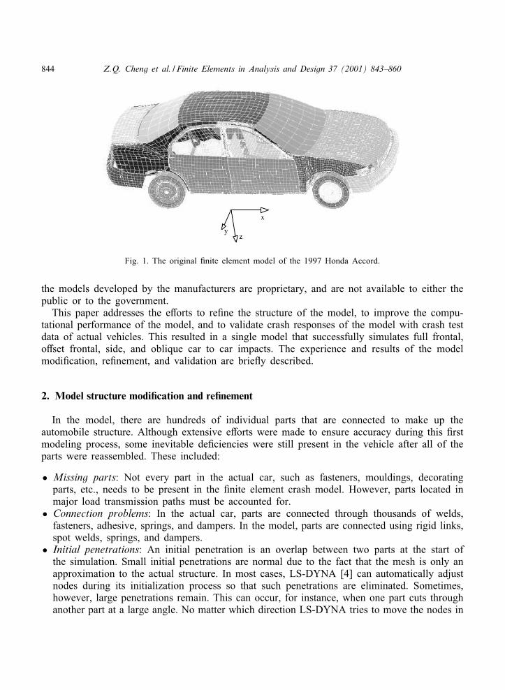
A "nite element model of a four-door 1997 Honda Accord DX Sedan, as shown inFig. 1, was created at the Automobile Safety Laboratory of the University of Virginia [5].The model was developed from data obtained from the disassembly and digitization of an ac-tual automobile using a reverse engineering technique. This approach was necessary because

∗ Corresponding author.E-mail address: [email protected] (W.D. Pilkey)

0168-874X/01/$ - see front matter ? 2001 Elsevier Science B.V. All rights reserved.PII: S 0168-874X(01)00071-3

844 Z.Q. Cheng et al. / Finite Elements in Analysis and Design 37 (2001) 843–860

Fig. 1. The original "nite element model of the 1997 Honda Accord.

the models developed by the manufacturers are proprietary, and are not available to either thepublic or to the government.

This paper addresses the e8orts to re"ne the structure of the model, to improve the compu-tational performance of the model, and to validate crash responses of the model with crash testdata of actual vehicles. This resulted in a single model that successfully simulates full frontal,o8set frontal, side, and oblique car to car impacts. The experience and results of the modelmodi"cation, re"nement, and validation are brie>y described.

2. Model structure modi�cation and re�nement

In the model, there are hundreds of individual parts that are connected to make up theautomobile structure. Although extensive e8orts were made to ensure accuracy during this "rstmodeling process, some inevitable de"ciencies were still present in the vehicle after all of theparts were reassembled. These included:

• Missing parts: Not every part in the actual car, such as fasteners, mouldings, decoratingparts, etc., needs to be present in the "nite element crash model. However, parts located inmajor load transmission paths must be accounted for.

• Connection problems: In the actual car, parts are connected through thousands of welds,fasteners, adhesive, springs, and dampers. In the model, parts are connected using rigid links,spot welds, springs, and dampers.

• Initial penetrations: An initial penetration is an overlap between two parts at the start ofthe simulation. Small initial penetrations are normal due to the fact that the mesh is only anapproximation to the actual structure. In most cases, LS-DYNA [4] can automatically adjustnodes during its initialization process so that such penetrations are eliminated. Sometimes,however, large penetrations remain. This can occur, for instance, when one part cuts throughanother part at a large angle. No matter which direction LS-DYNA tries to move the nodes in

Z.Q. Cheng et al. / Finite Elements in Analysis and Design 37 (2001) 843–860 845

question, a penetration will remain. Another situation can involve three shell layers that arenearly parallel and very close together. Resolving the penetration between the interior shelland one of the exterior shells can create new contacts with the other exterior shell. Casessuch as these must be corrected manually. Large penetrations result in high initial stresses inthe penetrated parts.

• Material property issues: There are over 200 parts in the model. While the material propertiesof the steel alloys are well known, the properties of some materials, such as honeycomb,foam, and plastics are not readily available. In particular, some of these materials undergolarge changes in volume when loaded, and exhibit highly non-linear behavior. These factorscan lead to some persistent computational problems.

The modi"cation and re"nement of the model is essentially a trial-and-error process whichcan be very ineOcient and time-consuming. In an e8ort to rectify the above issues, the followingprocedures are taken.

2.1. Static review

With the aid of the pre-processing software, HyperMesh [3], the model is reviewed staticallybefore the simulation is initiated. The issues dealt with during this review included:

• Element quality: Major issues related to one-dimensional elements (spot welds and rigid linksin particular for this model) include free-ends, rigid loops, dependency, connectivity, andduplicates. The issues associated with two- and three-dimensional elements involve elementwarpage, aspect ratio, skew, and Jacobian.

• Part association: This association indicates the connections (spot weld and rigid link) andrelative position (penetrated, attached, or separated). While penetrations can be manuallydetected using three-dimensional part viewing, a more eOcient way to "nd penetrations isby examining the initial stress distribution of the model prior to impact.

• Concentrated mass distribution: In the model, concentrated masses (point masses) were usedto represent parts like >uid reservoirs that are not substantial to impact load, test instrumenta-tion that is not in the primary crash zone, and anthromophic test devices that are not modeledin this study. Since high accelerations are generated during impact, inertial e8ects of pointmasses are very signi"cant.

• Summary information: Information such as the mass and the CG (center of gravity) of eachpart and the entire model can be found from the static review and is compared to the actualtest vehicle.

2.2. Initial stress check

The initialization of the model in a computational simulation provides information includingthe initial stress distribution. Using the initial stress distribution, one can easily identify theparts with large penetrations.


2.3. Gross motion

Gross motion reveals the overall dynamic response of the model and is akin to rigid bodymotion. The gross motion of the physical vehicle is found from the VHS video tape recordedby the National Highway TraOc Safety Administration (NHTSA) during each test. The com-parison of the gross motion of the test vehicle and computer model was used to initially de"nemajor problems. The gross motion of the vehicle also provides a simple way to detect parts orpart-group that are improperly connected to the main structure. While this motion reveals theglobal dynamic behavior of the vehicle, it is too coarse to be used for acceleration validation.

2.4. Acceleration responses

After all obvious problems in the model had been resolved, and the gross motion and de-formation of the model were similar to those of the test vehicles; the matching of accelerationresponses from the model with test signals became the central focus. Acceleration responses areavailable as output at all model nodes, but comparisons can only be made at locations instru-mented in the test. The standard locations for a full-frontal test are on the top and bottom ofthe engine, at the CG of the vehicle, and on the left and right sides of the rear cross member.

2.5. Post-test observations

Post-test observations (usually included in a NHTSA test report) provide information about thepermanent deformations at several locations of the tested vehicle. The permanent deformationscan also be reviewed from the test video. This information is useful for model modi"cation andre"nement, especially for those parts with large permanent deformations. During the validationof the model for side impact, the impact dynamic behavior of a movable deformable barrier(MDB) was of key importance. The post-crash deformations of the MDB model in computersimulations with the post-test observations of an actual side impact test [1] were utilized toimprove the MDB model structure and properly set the honeycomb material property fromwhich the impacting part of the MDB was constructed.

3. Computational issues of model simulations

Several major computational issues associated with LS-DYNA and the model need to beaddressed.

3.1. Negative volume of solid elements

Premature program termination due to the negative volume of solid elements was frequentlyencountered. Computationally, this is due to the calculation of the element Jacobian at geomet-ric points outside the boundary of highly deformed solid elements. If soft materials, such ashoneycomb and foam, were used for a solid element part, rapid compression of the elements


will likely result and negative volumes would be computed. The following parts of the Ac-cord model often caused negative volume problems resulting in premature termination of thesimulation:

• Radiator: a solid element part made from crushable foam.• Seat cushions: solid element parts made from low density foam.• The deformable barriers: solid element parts made from honeycomb material; used in sideimpact and o8set frontal impact simulations, respectively.

Major factors that are related to the improvement of the negative volume problem included:

• Element size: Computational experiments indicate that the smaller the element size of highlydeformed parts, the more likely the occurrence of negative volume calculations. Increasingelement size has proven to be an e8ective method in resolving this problem. Element sizehas an upper limit, however, if realistic modeling is to be accomplished.

• Material property: In a broad sense, the stress–strain relationship for the foam (low densityfoam and crushable foam) and honeycomb materials are de"ned by load curves. When therelative volume (the ratio of current to initial volume) of a solid element becomes very small,the slope of a load curve could be a major negative volume producing factor.

• Interior contact setting: Setting an interior contact for a solid element part is found toincrease the sti8ness of that part, which aids in reducing the negative volume problem forthat part. However, it seems reasonable that this setting would signi"cantly alter the impactbehavior of the part.

• Hourglass: One aspect that leads to negative volume problems is the deformation of elementsin an hourglass mode. Therefore, using the LS-DYNA solid element hourglass control helpsto avoid hourglass-mode deformations and thus reduce negative volume problems.

3.2. Shooting nodes

Another frequently occurring computational problem was a termination due to mass increase.That is, the percentage increase of the added mass has reached a prescribed limit. AlthoughLS-DYNA de"nes this termination as a normal termination, it usually happens before the com-pletion of the prescribed run time, or even at a very earlier stage of a simulation process. It isactually a computational instability. The animation of dynamic responses of the model showsthat the deformations of certain elements in one or more parts continue to increase to unrealis-tically large displacements. It appears as though certain nodes are ejecting or “shooting” out ofthe model as deformations develop. In LS-DYNA, the time step size roughly corresponds to thetransient time of an acoustic wave through an element using the shortest characteristic distance.Shooting nodes result in drastic decrease of the shortest element characteristic distance. Massscaling is done to meet the Courant time step size criterion [4]. The known factors that leadto, or have e8ects on, the shooting node problem are as follows.

• Poor mesh quality: In many cases, shooting nodes occur in poorly meshed parts. The partsthat have large warpage, skew ratios, and high aspect ratios are more likely to have shootingnodes. One explanation for this is that for nonlinear "nite element analysis, poor element


characteristics will more likely result in computational instabilities. Usually, after reconstruc-tion and improving mesh quality, shooting nodes disappear, but not always.

• Redundant elements: For the Accord model, the meshing of most parts was generated auto-matically from the digitized line and surface data. Due to errors and bias in the digitized data,redundant elements were sometimes created. If the nodes of a redundant element are not fullyconnected, that is, one or more nodes are freely ended, these nodes might displace wildlywhile the region of this part and this redundant element are deforming. Therefore, checkingfor, and removing, all redundant elements helps to avoid the shooting node problem.

• Hourglassing: To keep the computational time acceptable element formulation-2 in LS-DYNA(Belytschko–Tsay element) was used for most shell elements. The standard B-T elementis a four-node quadrilateral with a single Gaussian integration point at the center. Thisunder-integration can lead to the occurrence of zero-energy hourglass modes. A hourglassmode is another computational instability [2]. In some cases, the deformation of elementswith shooting nodes relates to an hourglass mode. The hourglass mode can be controlled byintroducing an arti"cial viscosity to damp out the oscillations [4]. Using the hourglass controlhas helped to eliminate shooting node problems. However, for the parts with poor meshingquality, redundant elements, and improper connections, using the hourglass control will onlydelay the occurrence of shooting nodes.

• Plastic failure of material: The primary material de"nition used in the model wasMAT−PIECEWISE−LINEAR−PLASTICITY. Usually, EPPF = 0 (plastic failure is not con-sidered) and TDEL = 0 (element will not be automatically deleted according to minimumtime step size) are set in the material card. This material selection was found to be ap-propriate for parts subject to compressive deformation. Some parts, however, were subjectto tensile deformation during the impact and shooting nodes were found more often in thismode. Under compression, parts are pressed together and cannot really “fail” the way theycan under tension; so it is appropriate to turn o8 the normal failure criteria. Under tension,however, it is not realistic to prevent failure since this can allow such a part to experienceextreme elongation which leads to shooting nodes. If plastic strain failure or minimum timestep size is set for these parts, the elements containing shooting nodes will be automaticallydeleted. This reduces added mass requirements and the computational process continues.

3.3. Energy balance

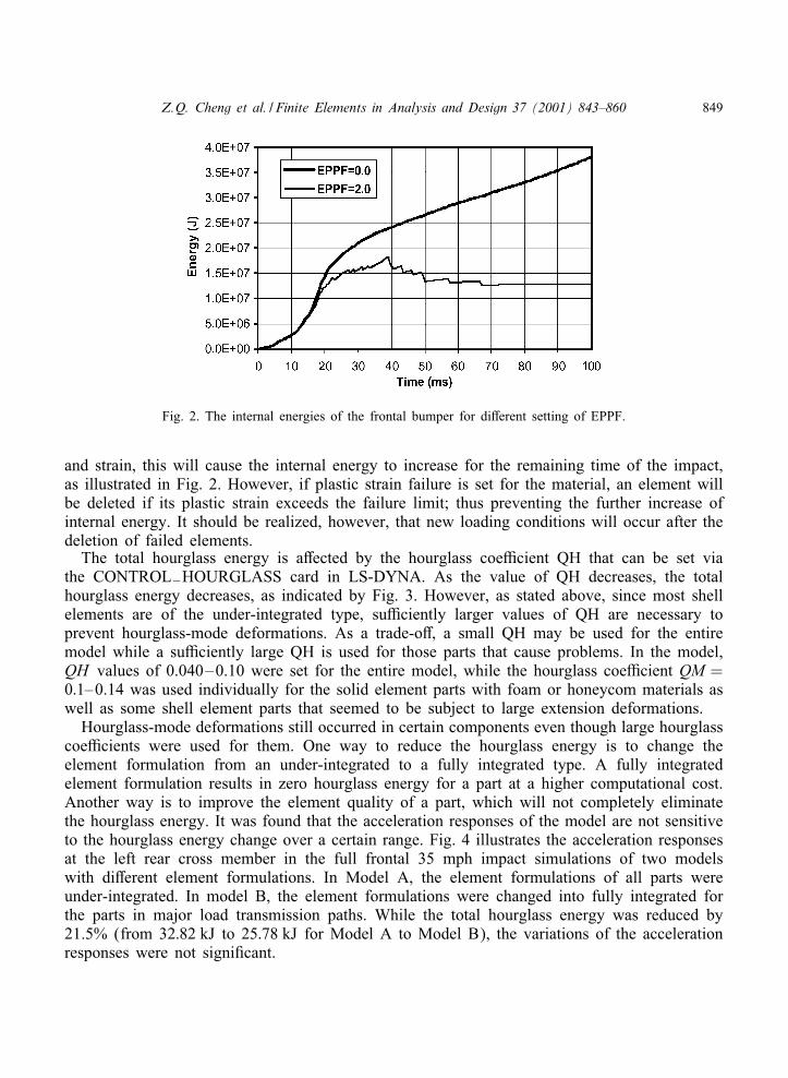
The overall model energy balance was used as a measure of FE model quality. Typically, itis thought that the increase of the total energy over the initial energy should be less than 10%and the ratio of the hourglass energy to the total energy be less than 10%. The increase ofthe total "nal internal energy over the total initial kinetic energy is a8ected by the de"nitionsof certain material properties in the model. Fig. 2 illustrates internal and kinetic energies ofthe front bumper in two cases. In one case, plastic failure is not considered (EPPF = 0 is setin the material card). In another case, the material fails when its plastic strain reaches 200%(EPPF = 2:0), and failed elements will be deleted automatically. The load curve (stress versusstrain) for this material usually remains >at in the plastic region. If plastic strain failure is notprescribed, once the stress reaches this plateau, the strain will continue to increase as long as aload is applied. Since the work done in deforming a part is proportional to the product of stress


Fig. 2. The internal energies of the frontal bumper for di8erent setting of EPPF.

and strain, this will cause the internal energy to increase for the remaining time of the impact,as illustrated in Fig. 2. However, if plastic strain failure is set for the material, an element willbe deleted if its plastic strain exceeds the failure limit; thus preventing the further increase ofinternal energy. It should be realized, however, that new loading conditions will occur after thedeletion of failed elements.

The total hourglass energy is a8ected by the hourglass coeOcient QH that can be set viathe CONTROL−HOURGLASS card in LS-DYNA. As the value of QH decreases, the totalhourglass energy decreases, as indicated by Fig. 3. However, as stated above, since most shellelements are of the under-integrated type, suOciently larger values of QH are necessary toprevent hourglass-mode deformations. As a trade-o8, a small QH may be used for the entiremodel while a suOciently large QH is used for those parts that cause problems. In the model,QH values of 0.040–0.10 were set for the entire model, while the hourglass coeOcient QM =0:1–0.14 was used individually for the solid element parts with foam or honeycom materials aswell as some shell element parts that seemed to be subject to large extension deformations.

Hourglass-mode deformations still occurred in certain components even though large hourglasscoeOcients were used for them. One way to reduce the hourglass energy is to change theelement formulation from an under-integrated to a fully integrated type. A fully integratedelement formulation results in zero hourglass energy for a part at a higher computational cost.Another way is to improve the element quality of a part, which will not completely eliminatethe hourglass energy. It was found that the acceleration responses of the model are not sensitiveto the hourglass energy change over a certain range. Fig. 4 illustrates the acceleration responsesat the left rear cross member in the full frontal 35 mph impact simulations of two modelswith di8erent element formulations. In Model A, the element formulations of all parts wereunder-integrated. In model B, the element formulations were changed into fully integrated forthe parts in major load transmission paths. While the total hourglass energy was reduced by21.5% (from 32:82 kJ to 25:78 kJ for Model A to Model B), the variations of the accelerationresponses were not signi"cant.


Fig. 3. The variation of the total hourglass energy vs. QH.

Fig. 4. Comparison between fully and under integrated element formulations (left rear cross member).

Fig. 5. Acceleration calculation using rigid body acceleration data (left rear cross member in four repeated simula-tions).


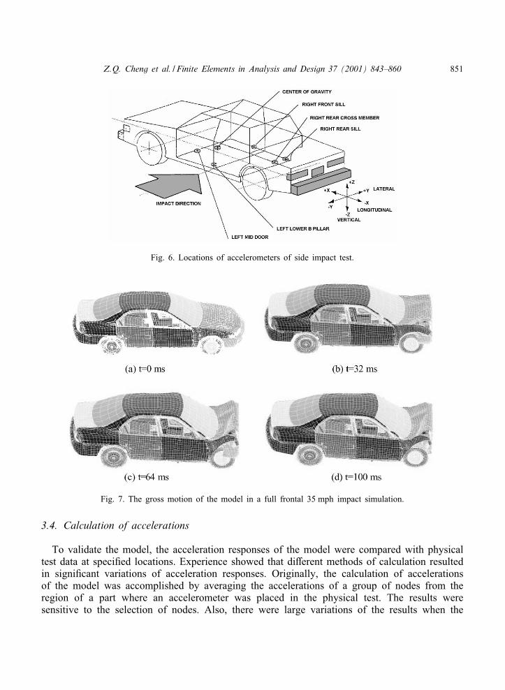
Fig. 6. Locations of accelerometers of side impact test.

Fig. 7. The gross motion of the model in a full frontal 35 mph impact simulation.

3.4. Calculation of accelerations

To validate the model, the acceleration responses of the model were compared with physicaltest data at speci"ed locations. Experience showed that di8erent methods of calculation resultedin signi"cant variations of acceleration responses. Originally, the calculation of accelerationsof the model was accomplished by averaging the accelerations of a group of nodes from theregion of a part where an accelerometer was placed in the physical test. The results weresensitive to the selection of nodes. Also, there were large variations of the results when the


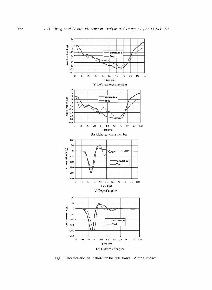
Fig. 8. Acceleration validation for the full frontal 35 mph impact.


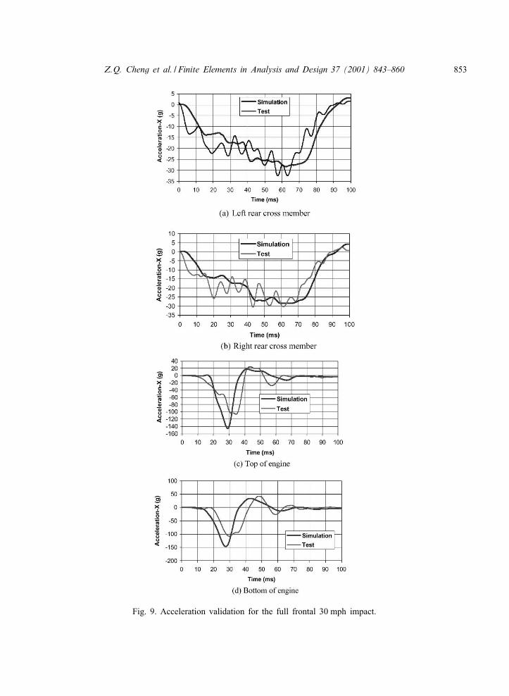
Fig. 9. Acceleration validation for the full frontal 30 mph impact.


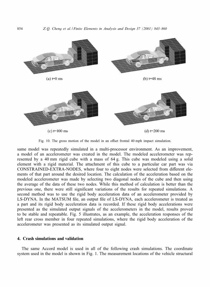
Fig. 10. The gross motion of the model in an o8set frontal 40 mph impact simulation.

same model was repeatedly simulated in a multi-processor environment. As an improvement,a model of an accelerometer was created in the model. The modeled accelerometer was rep-resented by a 40 mm rigid cube with a mass of 64 g. This cube was modeled using a solidelement with a rigid material. The attachment of this cube to a particular car part was viaCONSTRAINED-EXTRA-NODES, where four to eight nodes were selected from di8erent ele-ments of that part around the desired location. The calculation of the acceleration based on themodeled accelerometer was made by selecting two diagonal nodes of the cube and then usingthe average of the data of these two nodes. While this method of calculation is better than theprevious one, there were still signi"cant variations of the results for repeated simulations. Asecond method was to use the rigid body acceleration data of an accelerometer provided byLS-DYNA. In the MATSUM "le, an output "le of LS-DYNA, each accelerometer is treated asa part and its rigid body acceleration data is recorded. If these rigid body accelerations werepresented as the simulated output signals of the accelerometers in the model, results provedto be stable and repeatable. Fig. 5 illustrates, as an example, the acceleration responses of theleft rear cross member in four repeated simulations, where the rigid body acceleration of theaccelerometer was presented as its simulated output signal.

4. Crash simulations and validation

The same Accord model is used in all of the following crash simulations. The coordinatesystem used in the model is shown in Fig. 1. The measurement locations of the vehicle structural


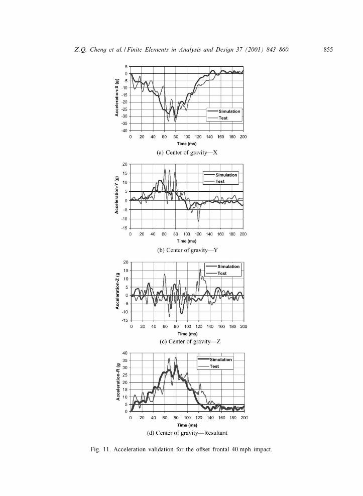
Fig. 11. Acceleration validation for the o8set frontal 40 mph impact.


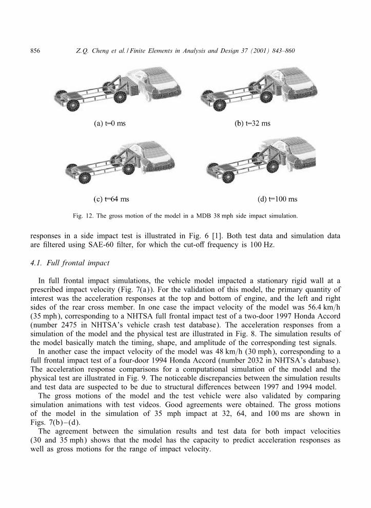
Fig. 12. The gross motion of the model in a MDB 38 mph side impact simulation.

responses in a side impact test is illustrated in Fig. 6 [1]. Both test data and simulation dataare "ltered using SAE-60 "lter, for which the cut-o8 frequency is 100 Hz.

4.1. Full frontal impact

In full frontal impact simulations, the vehicle model impacted a stationary rigid wall at aprescribed impact velocity (Fig. 7(a)). For the validation of this model, the primary quantity ofinterest was the acceleration responses at the top and bottom of engine, and the left and rightsides of the rear cross member. In one case the impact velocity of the model was 56:4 km=h(35 mph), corresponding to a NHTSA full frontal impact test of a two-door 1997 Honda Accord(number 2475 in NHTSA’s vehicle crash test database). The acceleration responses from asimulation of the model and the physical test are illustrated in Fig. 8. The simulation results ofthe model basically match the timing, shape, and amplitude of the corresponding test signals.

In another case the impact velocity of the model was 48 km=h (30 mph), corresponding to afull frontal impact test of a four-door 1994 Honda Accord (number 2032 in NHTSA’s database).The acceleration response comparisons for a computational simulation of the model and thephysical test are illustrated in Fig. 9. The noticeable discrepancies between the simulation resultsand test data are suspected to be due to structural di8erences between 1997 and 1994 model.

The gross motions of the model and the test vehicle were also validated by comparingsimulation animations with test videos. Good agreements were obtained. The gross motionsof the model in the simulation of 35 mph impact at 32, 64, and 100 ms are shown inFigs. 7(b)–(d).

The agreement between the simulation results and test data for both impact velocities(30 and 35 mph) shows that the model has the capacity to predict acceleration responses aswell as gross motions for the range of impact velocity.


4.2. OAset frontal impact

In the o8set frontal impact, 40% of the vehicle width overlapped a honeycomb barrier andimpacted it at 63:9 km=h (40 mph), as illustrated by Fig. 10(a). The barrier, supplemented witha ground plane, was stationary and deformable. The barrier was made of honeycomb materialand wrapped with sheet metal.

The data of NHTSA test No. 2286 were used to validate simulation results. The physicaltest was conducted by the Insurance Institute for Highway Safety and the data were providedto NHTSA. Only the acceleration at the CG location of the vehicle was measured in the test.The simulation results and test data are displayed in Fig. 11(a)–(d) where the resultant andx-direction accelerations from the simulation and the test are in good agreement. The resultantacceleration needs to be computed because of the rigid body rotation of the vehicle during theimpact. LS-DYNA outputs rigid body accelerations in the global coordinate system whereas thephysical test recorded accelerations in the local coordinate system corresponding to the mountingof the accelerometer.

The gross motions of the model and the vehicle were also compared. The gross motions ofthe model are displayed in Figs. 10(b)–(d) for the 48, 100, 200 ms time-points.

4.3. Side impact

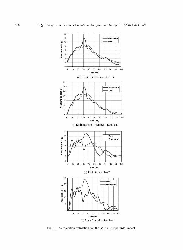
In the side impact simulations, the model was initially stationary and was impacted by aMDB that is traveling toward the vehicle at an initial velocity of 27:7 km=h (17:3 mph) in thex-direction and 54.3 (33:9 mph) in the y-direction (Fig. 12(a)). The corresponding physical testwas a NHTSA side impact test of a four-door 1997 Honda Accord DX Sedan (Number 2479).The acceleration responses at the locations of vehicle’s CG, front and rear right sill, and rightrear cross member were used for validation. The simulation results and test signals for the rightrear cross member and right front sill are illustrated in Figs. 13(a)–(d). It can be seen that iny-direction, the simulation results match well with the test results. The gross motions of themodel are shown in Figs. 12(b)–(d) for the 32, 64, and 100 ms time-points.

It is concluded that the impact dynamic characteristics and kinematic behavior of the MDBhave signi"cant e8ects on the results of side impact simulations.

4.4. Oblique impact by a Ford Explorer

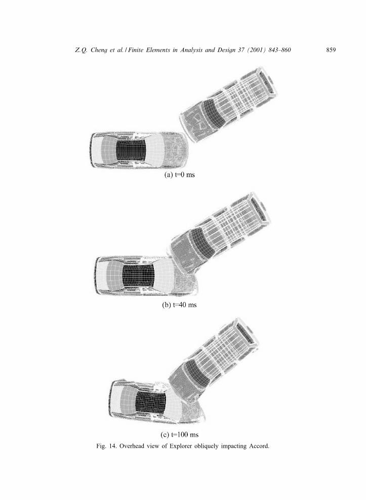
In this simulation, the Accord model was impacted frontally by the Explorer model at a 30◦

oblique angle from the center line, as shown in Fig 14(a). The Explorer model was developedby Oak Ridge National Laboratory. The initial velocities for the Accord model were vx =56:5 km=h (35:3 mph); vy = 0, and vz = 0. The initial velocities for the Explorer model werevx=−48:5 km=h (30:3 mph); vy=28 km=h (17:5 mph), and vz =0. The simulation was run for100 ms. Figs. 14 (a)–(c) are overhead views of the Explorer obliquely impacting Accord at0,40, and 100 ms.


Fig. 13. Acceleration validation for the MDB 38 mph side impact.


Fig. 14. Overhead view of Explorer obliquely impacting Accord.


5. Concluding remarks

A single "nite element crash model has been developed for a four-door 1997 Honda AccordDX Sedan. This model has been successfully used in the simulations of the full frontal, o8setfrontal, side, and oblique car-to-car impacts. The results of computational simulations werevalidated with test data of actual vehicles. The validation indicates that the model is suitablefor use as a crash partner for other vehicles. Computational tests of the model show that themodel is computationally stable, reliable, and repeatable.

Acknowledgements

The work of developing a "nite element model of the four-door 1997 Honda Accord DXSedan was sponsored by the US National Highway TraOc Safety Administration (NHTSA). Thiswas part of a joint industry–government program: Partnership for New Generation Vehicles.

References

[1] J. Fleck, New Car Assessment Program=Side Impact Testing=Passenger Cars=1997 Honda Accord=4-Door Sedan,NHTSA Report No. 214-MGA-97-01, MGA Research Corporation, WI, 1996.

[2] T.J.R. Hughes, The Finite Element Method, Linear Static and Dynamic Finite Element Analysis, Prentice-Hall,Inc., Englewood Cli8s, NJ, 1987.

[3] HyperMesh User’s Manual, Version 2.1, Altair Computing, Inc., 1997.[4] Livermore Software Technology Corporation, LS-DYNA Keyword User’s Manual, Nonlinear Dynamic Analysis

of Structures, Livermore, CA, 1999.[5] J.G. Thacker, S.W. Reagan, J.A. Pellettiere, W.D. Pilkey, J.R. Crandall, E.M. Sieveka, Experiences during

development of a dynamic crash response automobile model, Finite Element Anal. Des. 30 (1998) 279–295.

Experiences in reverse-engineering of a nite element...

Documents

Transcript of Experiences in reverse-engineering of a nite element...