Computer Science Department of The University of AucklandCITR at Tamaki Campus (http://www.citr.auckland.ac.nz)

CITR-TR-102 October 2001

Experience with Optical Flow in Colour Video ImageSequences

John Barron1 and Reinhard Klette2

Abstract

The paper studies optical flow methods on colour frames captured by adigital video camera. The paper reviews related work, specifies somenew colour optical flow constraints and reports on experimentalevaluations for one image sequence.

1 Department of Computer Science, University of Western Ontario, London, Ontario, Canada, N6A5B7, barron@csd.uwo.ca2 Center for Image Technology and Robotics Tamaki Campus, The University of Auckland, Auckland,New Zealand. r.klette@auckland.ac.nz

You are granted permission for the non-commercial reproduction, distribution, display, and performance of this technical reportin any format, BUT this permission is only for a period of 45 (forty-five) days from the most recent time that you verified thatthis technical report is still available from the CITR Tamaki web site under terms that include this permission. All other rightsare reserved by the author(s).

Experience with Optical Flow in Colour Video Image Sequences

John Barron�and Reinhard Klette

y

Abstract

The paper studies optical ow methods on colour

frames captured by a digital video camera. The paper

reviews related work, speci�es some new colour optical

ow constraints and reports on experimental evalua-

tions for one image sequence.

1 Introduction

Consider colour images C1, C2, : : : Cn capturedas n consecutive images of a video sequence where thecamera is moving. An important problem consists inmeasuring image displacements between pairs of con-

secutive images using optical ow. Assume that onescene point P = (X;Y; Z) is projected onto imageCt(x; y) at time t and onto Ct+1(x + ud; y + vd) attime t+Æt. The vector ud = (ud; vd)

T is the image dis-placement of the projected scene point P = (X;Y; Z),and it will be estimated by calculating optical ow

ue = (ue; ve)T using the given colour value distribu-

tions in Ct and Ct+1, and possibly further image dataof the captured sequence. The ideal solution would beud = ue.

2 Review

The literature reporting on optical ow from colourimages is quite sparse, despite the fact that multispec-tral approaches have been suggested already for about

twenty years. Markandey and Flinchbaugh [5] haveproposed a multispectral approach for optical ow com-putation. Their two-sensor proposal is based on solvinga system of two linear equations having both optical ow components as unknowns. The equations are thestandard optical ow constraints

@E

@x

u+@E

@y

v +@E

@t

= 0; (1)

�Department of Computer Science, University of Western On-

tario, London, Ontario, Canada, N6A 5B7, barron@csd.uwo.cayCITR, University of Auckland, Tamaki Campus, Building

731 Auckland, New Zealand, r.klette@auckland.ac.nz

where E is one image channel, formulated for eachchannel separately. Their experiments use colour TVcamera data and a combination of infrared and visibleimagery. In each experiment the data was smoothed byconvolution with a Gaussian of � = 2:0 before calcula-tion of the derivatives and the calculated vector �eldswere post-processed using 10 iterations of median �l-tering, followed by 100 iterations of the vector �eldsmoothing technique described by Schunck [7]. Theirexperiments have shown that \vector �eld smoothing

played a signi�cant role in the computation of optical

ow" for two-channel imagery. The condition numberof the integration matrix for the system of linear equa-tions is used for estimating numerical stability.

Golland and Bruckstein [1] follow the same algebraicmethod. They compare a straightforward 3-channelapproach using RGB data with two 2-channel meth-ods, the �rst based on normalized RGB values andthe second based on a special hue-saturation de�nition.The standard optical ow constraint may be applied toeach one of the RGB quantities, providing an overde-termined system of linear equations:

@R

@x

u+@R

@y

v +@R

@t

= 0 ; (2)

@G

@x

u+@G

@y

v +@G

@t

= 0 ; (3)

@B

@x

u+@B

@y

v +@B

@t

= 0 : (4)

The solution for the optical ow may be found by usinga pseudo-inverse computation:

u =�A

TA��1

ATb (5)

where:

A =

0@ Rx Ry

Gx Gy

Bx By

1A

; b =

0@ �Rt

�Gt

�Bt

1A (6)

The matrix A must be non-singular. The smallesteigenvalue of AT

A or the condition number of ATA

can be used to measure numerical stability, i.e. if the

1

Figure 1. (Left) The original video 720 � 576 colour image and (Right) the even interpolated colourimage. The odd interpolated colour image looks about the same but is translated by about (-3,0) withrespect to the even image.

smallest eigenvalue is below a threshold or the con-dition number is above a threshold, then we set u

to be unde�ned at this image location. We imple-ment Golland and Bruckstein's method with weightsfor each channel in a standard least squares frame-work. If we assume a constant ow vector in a(2n+1)�(2n+1) then AT

A becomes the least squaresLucas and Kanade optical ow method [4, 8]. We usen = 1 for the Lucas and Kanade results reported here.If all weights were 0 except for the Y channel (withvalue 1) then we would have the standard Lucas andKanade calculation [4, 8]. If the R, G and B weightsare 1 with all other weights 0 we have colour Lucasand Kanade. Note that Y=0.299R+0.587G+0.114B,so if we changed the non-zero weights to these valueswe would obtain exactly the same results as for the Yimages. Lastly, if n = 1, we have the standard Gollandand Bruckstein method.

We recast the standard Horn and Schunck regular-ization [2, 8, 9] as the minimisation of:

nXi

wi [Exiu+ Eyiv +Eti]2+ �

2(u2x+ u

2y+ v

2x+ v

2y):

The weights wi indicate the attached importance ofeach channel of image information, e.g., wi = 0 meanschannel i has absolutely no importance. If all wi are0 except the one corresponding to the Y channel (withvalue 1) and � = 0 then this minimisation is exactlyHorn and Schunck on a grayvalue image [2, 8].

Golland and Bruckstein [1] have reported that theRGB-method \provides suÆcient quality for velocity

estimates when the object undergoes translations in a

plane parallel to the image plane, but if more com-

plex kinds of motion are involved, this method, like

any other using the brightness conservation assump-

tion, produces estimates with signi�cant errors." Fur-thermore, their methods \provide much more precise

information about the object motion." However, thesestatements have been deducted from a very small num-ber of experiments, and more detailed studies mightbe worthwhile. In general, optical ow computed for asingle image point has proved unsuccessful, local neigh-bourhoods under some parametric constraint (such asconstant velocity) or global regularization of a func-tional is necessary to obtain useful ow.

Ohta [6] derives optical ow equations in a leastsquares framework on channel derivatives in colour im-ages. Let Exi and Eyi denote the x and y derivativesin colour channel i. For example Ex5 could be the x

derivatives in the hue image. Ohta assumes that thereare n � 2 optical ow constraints for the di�erent chan-nels. For n = 2, it follows

u =Ey1Et2 � Et1Ey2

Ex1Ey2 � Ey1Ex2

and v =Et1Ex2 � Ex1Et2

Ex1Ey2 � Ey1Ex2

:

Both equations are solvable if Ex1Ey2 � Ey1Ex2 6= 0.Letting the error in the i-th equation be ei, taking thesum of all squared errors for all n equations, calculat-ing its partial derivatives with respect to u and v, and

Figure 2. (Left) The Horn and Schunck flow for the Y image with � = 3 and 100 iterations and post-thresholding of jjrIjj2 > 5:0 and (Right) the Lucas and Kanade for for the Y image with smallesteigenvalue thresholding of � > 5:0.

Figure 3. (Left) The Horn and Schunck flow for the saturation image with � = 3 and 100 iterations andpost-thresholding of jjrIjj2 > 5:0 and (Right) the Lucas and Kanade for for the Y image with smallesteigenvalue thresholding of � > 5:0.

letting these formulae be equal to zero, we obtain [6]

u =

PExiEyi

PEyiEti �

PE2yi

PExiEtiP

E2xi

PE2yi� (P

ExiEyi)2

(7)

v =

PExiEyi

PExiEti �

PE2xi

PEyiEtiP

E2xi

PE2yi� (P

ExiEyi)2

;(8)

where summations are from 1 to n. This approach andthe generalized inverse method [1, 5] assume constantweights for all equations. Our implementation allowsus to set arbitrary weights for each of the nine RGB,HSI and YIQ colour channels. Note that if all weights

are zero except for the Y channel weight being 1, thenin a (2n+1)� (2n+1) we again have a standard Lucasand Kanade [4, 8] least squares calculation.

3 New Approach

In a new approach, we recast the standard Horn andSchunck regularization as the minimisation of:

nXi

wi [Exiu+Eyiv +Eti]2 + �

2fd(u; v): (9)

Figure 4. (Left) Standard Golland and Bruckstein flow and (Right) least squares Golland and Bruck-stein flow, both with post-thresholding of jjrIjj2 > 5:0.

Figure 5. (Left) Colour Ohta flow and (Right) saturation/Y Ohta flow, both with post-thresholding ofjjrIjj2 > 5:0.

Again, as for the Horn and Schunck regularization, theweights wi indicate the attached importance of eachchannel of image information and can be set so as toinclude/exclude any colour channel. fd(u; v) is a direc-tional constraint that depends on one knowing whetherthe camera is panning or zooming. Because the 3Dtranslational direction is known, the direction of owcan be computed everywhere using the standard opti-cal ow equations [3] and this can be used to constrainthe minimisation. The directional constraint can beexpressed as:

fd(u; v) = (u � ud)2� jjujj

22jjudjj

22 = 0; (10)

where, because due to sensor motion is only translationand can be written as [3] ud can be written as:

ud =

�ud

vd

�= � � jj(x; y; f)jj2 �A(x;y)m̂; (11)

where (x; y) is an image location, � is the relative

depth, i.e. � =jjmjj

jj(X;Y;Z)jj2, jjmjj is the (unknown)

sensor translation magnitude and (X;Y; Z) are the 3Dcoordinates of some 3D moving point projected onto(x; y). Note that since we do not know �, ud is only inthe direction of the true optical ow vector and scaledby the � value used. We can write A(x;y), a 2 � 3 ma-

Figure 6. (Left) Colour Horn and Schunck flow with � = 3 and (Right) colour Barron and Klette flowwith � = 1:0, both with post-thresholding of jjrIjj2 > 5:0 and 100 iterations.

Figure 7. (Left) Barron and Klette flow for the Y and saturation images and (Right) Barron and Kletteflow for the Y image only, both with post-thresholding of jjrIjj2 > 5:0 and 100 iterations and � = 1:0.

trix, as:

A(x;y) =

��f 0 x

0 �f y

�; (12)

where f is the e�ective focal length (determined em-pirically to be about 40mm).

4 Experiments

This paper reports on an experimental evaluation ofthese 4 approaches [Golland and Bruckstein, Ohta, andBarron and Klette with Horn and Schunck and Lucasand Kanade serving as a standards] for optical ow in

colour video images using various values for the wi'sand � = 3 and � = 1. We show that sometimes opti-cal ow results improve for non-zero weights (multiplecolour image channels). Our � and � values producedthe best results. Our investigation consists of a a qual-itative evaluation of these algorithms on real colourvideo image sequences.

Figure 1a shows an original interlaced video image.There is motion of about 3 pixels to the right betweenthe even and odd lines of the image. We generate 2images from this single image. Figure 1b show the im-age generated by linearly interpolating the even lines,another second image is generated by linearly interpo-

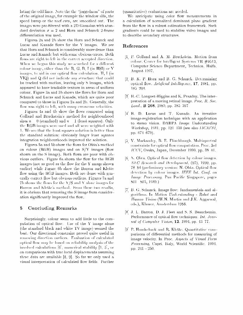
lating the odd lines. Note the the \jaggedness" of partsof the original image, for example the window sills, thespeed bump or the roof eves, are smoothed out. Theimages were pre-�ltered with a 2D Gaussian with stan-dard deviation � = 2 and Horn and Schunck 2-framedi�erentiation was used.

Figures 2a and 2b show the Horn and Schunck andLucas and Kanade ows for the Y images. We seethat Horn and Schunck is considerably more dense thanLucas and Kanade but with some obvious errors. Both ows are right to left in the correct accepted direction.When we began this study we searched for a di�erentcolour image, other than the R, G, B, I (in HSI) or Yimages, to aid in our optical ow calculation. H, I (inYIQ) and Q did not indicate any structure that couldbe tracked with motion, leaving only S images, whichappeared to have trackable texture in areas of uniformcolour. Figure 3a and 3b shows the ows for Horn andSchunck and Lucas and Kanade, which are quite poorcompared to those in Figures 2a and 2b. Generally, the ow was right to left, with many erroneous velocities.

Figures 4a and 4b show the ows computed usingGolland and Bruckstein's method for neighbourhoodsizes n = 0 (standard) and n = 1 (least squares). Onlythe RGB images were used and all were weighted with1. We see that the least squares solution is better thanthe standard solution; obviously larger least squaresintegration neighbourhoods improved the solution.

Figures 5a and 5b show the ows for Ohta's methodon colour (RGB) images and on S/Y images ( owshown on the S image). Both ows are poor with ob-vious outliers. Figure 6a shows the ow for the RGBimages (not as good as the ow for the Y image shownearlier) while Figure 6b show the Barron and Klette ow using the RGB images. Both are dense with gen-erally correct ow but obvious outliers. Figures 7a and7b shows the ows for the Y/S and Y alone images forBarron and Klette's method. From these two results,it is obvious that removing the S image from consider-ation signi�cantly improved the ow.

5 Concluding Remarks

Surprisingly, colour seem to add little to the com-putation of optical ow. Use of the Y image alone(the standard black and white TV image) seemed thebest. Our directional constraint proved quite useful inremoving direction outliers. Evaluation of calculatedoptical ow may be based on reliability analysis of theinvolved calculations [6], numerical stability [1, 5], oron comparisons with true local displacements assumingthese data are available [8, 9]. So far we only used avisual interpretation of calculated ow �elds. Further

(quantitative) evaluations are needed.We anticipate using color ow measurements in

a calculation of normalized dominant plane gradientfrom the ow in a robust estimation framework. Suchgradients could be used to stabilise video images andto describe secondary structures.

References

[1] P. Golland and A. M. Bruckstein. Motion fromcolour. Center for Intelligent Systems TR #9513,Computer Science Department, Technion, Haifa,August 1997.

[2] B. K. P. Horn and B. G. Schunck. Determiningoptical ow. Arti�cial Intelligence, 17, 1981, pp.185{204.

[3] H.-C. Longuet-Higgins and K. Prazdny. The inter-pretation of a moving retinal image. Proc. R. Soc.Lond., B 208, 1980, pp. 385{397.

[4] B. D. Lucas and T. Kanade. An iterativeimage-registration technique with an applicationto stereo vision. DARPA Image Understanding

Workshop, 1981, pp. 121{130 (see also IJCAI'81,pp. 674{679).

[5] V. Markandey, B. E. Flinchbaugh. Multispectralconstraints for optical ow computation. Proc. 3rdICCV, Osaka, Japan, December 1990, pp. 38{41.

[6] N. Ohta. Optical ow detection by colour images.NEC Research and Development, (97), 1990, pp.78{84 (preliminary version: N. Ohta. Optical owdetection by colour images. IEEE Int. Conf. on

Image Processing, Pan Paci�c Singapore, pages801 {805, 1989.)

[7] B. G. Schunck. Image ow: fundamentals and al-gorithms. In Motion Understanding - Robot and

Human Vision (W.N. Martin and J.K. Aggarwal,eds.), Kluwer, Amsterdam 1988.

[8] J. L. Barron, D. J. Fleet and S. S. Beauchemin.

Performance of optical ow techniques. Int. Jour-nal of Computer Vision, 12, 1994, pp. 43{77.

[9] P. Handschack and R. Klette. Quantitative com-parisons of di�erential methods for measuring ofimage velocity. In Proc. Aspects of Visual Form

Processing, Capri, Italy, World Scienti�c, 1994,pp. 241 - 250.