Expansions g eom etriques et ampleur - CORE · de vu de la logique du premier ordre, c’est à...
89
Expansions g´ eom´ etriques et ampleur Juan Felipe Carmona To cite this version: Juan Felipe Carmona. Expansions g´ eom´ etriques et ampleur. G´ eom´ etrie alg´ ebrique [math.AG]. Universit´ e Claude Bernard - Lyon I, 2015. Fran¸cais. <NNT : 2015LYO10067>. <tel- 01229377> HAL Id: tel-01229377 https://tel.archives-ouvertes.fr/tel-01229377 Submitted on 26 Nov 2015 HAL is a multi-disciplinary open access archive for the deposit and dissemination of sci- entific research documents, whether they are pub- lished or not. The documents may come from teaching and research institutions in France or abroad, or from public or private research centers. L’archive ouverte pluridisciplinaire HAL, est destin´ ee au d´ epˆ ot et ` a la diffusion de documents scientifiques de niveau recherche, publi´ es ou non, ´ emanant des ´ etablissements d’enseignement et de recherche fran¸cais ou ´ etrangers, des laboratoires publics ou priv´ es.
Transcript of Expansions g eom etriques et ampleur - CORE · de vu de la logique du premier ordre, c’est à...

Expansions geometriques et ampleur
Juan Felipe Carmona
To cite this version:
Juan Felipe Carmona. Expansions geometriques et ampleur. Geometrie algebrique [math.AG].Universite Claude Bernard - Lyon I, 2015. Francais. <NNT : 2015LYO10067>. <tel-01229377>
HAL Id: tel-01229377
https://tel.archives-ouvertes.fr/tel-01229377
Submitted on 26 Nov 2015
HAL is a multi-disciplinary open accessarchive for the deposit and dissemination of sci-entific research documents, whether they are pub-lished or not. The documents may come fromteaching and research institutions in France orabroad, or from public or private research centers.
L’archive ouverte pluridisciplinaire HAL, estdestinee au depot et a la diffusion de documentsscientifiques de niveau recherche, publies ou non,emanant des etablissements d’enseignement et derecherche francais ou etrangers, des laboratoirespublics ou prives.

UNIVERSITÉ CLAUDE BERNARD- LYON 1INSTITUT CAMILLE JORDAN
UNIVERSIDAD DE LOS ANDES
GEOMETRIC EXPANSIONS ANDAMPLENESS
EXPANSIONS GÉOMÉTRIQUES ET AMPLEUR
by
Juan Felipe Carmona
A thesis submitted in partial fulfillment for thedegree of Doctor of Philosophy
inMathematics
in theGraduate Division
Mathematics Department
May 2015

N° d’ordre 2015-67
UNIVERSITÉ CLAUDE BERNARD- LYON 1
INSTITUT CAMILLE JORDAN
UNIVERSIDAD DE LOS ANDES
pour l’obtention
du DIPLOME DE DOCTORAT
(arrêté du 7 août 2006)
soutenance le 10 / 06 / 2015
par
Juan Felipe Carmona
GEOMETRIC EXPANSIONS AND AMPLENESS
Directeur de thèse: Martin-Pizzarro, Amador
JURY : Enrique Casanovas
Alex Berenstein
John Goodrick
Chris Lawskoski
Amador Martin-Pizarro
Frank Wagner

Declaration of Authorship
I, JUAN FELIPE CARMONA, declare that this thesis titled, ‘GEOMETRIC EXPAN-
SIONS AND AMPLENESS’ and the work presented in it are my own. I confirm that:
Signed:
Date:
i

Reason with its use of language has set up a satisfactory architecture, like the delightful,
rhythmical composition in Renaissance painting.
Julio Cortázar.

UNIVERSITÉ CLAUDE BERNARD- LYON 1
INSTITUT CAMILLE JORDAN
UNIVERSIDAD DE LOS ANDES
Résumé / AbstractGraduate Division
Mathematics Department
Doctor of Philosophy
in
Mathematics
by Juan Felipe Carmona
Le résultat principal de cette thèse est l’étude de l’ampleur dans des expansion des struc-
tures géométriques et de SU-rang omega par un prédicat dense/codense indépendant. De
plus, nous étudions le rapport entre l’ampleur et l’équationalité, donnant une preuve dir-
ecte de l’équationalité de certaines théories CM-triviales. Enfin, nous considérons la
topologie indiscernable et son lien avec l’équationalité et calculons la complexité indis-
cernable du pseudoplan libre.
The main result of this thesis is the study of how ampleness grows in geometric and
SU -rank omega structures when adding a new independent dense/codense subset. In
another direction, we explore relations of ampleness with equational theories; there, we
give a direct proof of the equationality of certain CM-trivial theories. Finally, we study
indiscernible closed sets—which are closely related with equations—and measure their
complexity in the free pseudoplane.

Acknowledgements
I would like to thank Alexander Berenstein and Amador Martín-Pizarro for their guidance
and mostly for their patience. They are great tutors and excellent friends. I am grateful
to the Bogotá logic group and to the Lyon logic group, specially to my friends Haydar
Göral and Tomás Ibarlucía, who were very supportive while I was in Lyon. I am grateful
also to my dear friend Isabel Müller for the time we spent in Berlin and in Lyon discussing
mathematics. Finally I would like to thank Xavier Caicedo, who introduced me to model
theory, I am very grateful to him for keep reminding me that mathematical logic is
beautiful.
iv

Contents
Declaration of Authorship i
Abstract iii
Acknowledgements iv
Introduction en français 1
Introduction 7
1 Preliminaries 131.1 Conventions . . . . . . . . . . . . . . . . . . . . . . . . . . . . . . . . . . . 131.2 Imaginaries . . . . . . . . . . . . . . . . . . . . . . . . . . . . . . . . . . . 141.3 Independence on strongly minimal theories . . . . . . . . . . . . . . . . . . 151.4 Simple and stable theories . . . . . . . . . . . . . . . . . . . . . . . . . . . 181.5 Forking and canonical bases . . . . . . . . . . . . . . . . . . . . . . . . . . 211.6 One-basedness . . . . . . . . . . . . . . . . . . . . . . . . . . . . . . . . . 24
2 Ampleness 272.1 CM-triviality . . . . . . . . . . . . . . . . . . . . . . . . . . . . . . . . . . 272.2 Ampleness . . . . . . . . . . . . . . . . . . . . . . . . . . . . . . . . . . . . 282.3 Weak ampleness . . . . . . . . . . . . . . . . . . . . . . . . . . . . . . . . 31
3 Geometric structures with a dense independent subset 383.1 Independent predicates in geometric theories . . . . . . . . . . . . . . . . . 383.2 Ampleness . . . . . . . . . . . . . . . . . . . . . . . . . . . . . . . . . . . . 41
4 Structure of SU-rank ω with a dense independent subset of generics 504.1 Structure of SU-rank ω with a dense independent subset of generics . . . . 504.2 Ampleness . . . . . . . . . . . . . . . . . . . . . . . . . . . . . . . . . . . . 54
5 Equationality 615.1 Equational theories and equations . . . . . . . . . . . . . . . . . . . . . . . 625.2 CM-triviality and equationality . . . . . . . . . . . . . . . . . . . . . . . . 655.3 The indiscernible closure . . . . . . . . . . . . . . . . . . . . . . . . . . . . 675.4 The free pseudoplane . . . . . . . . . . . . . . . . . . . . . . . . . . . . . . 69
v
Contents vi
Bibliography 77

Introduction en français
La théorie des modèles a ses origines dans l’étude des structures mathématiques de point
de vu de la logique du premier ordre, c’est à dire, dans un langage finitaire tel que l’on
quantifie sur des éléments mais pas sur des sous-parties arbitraires de la structure (Ces
restrictions, qui étaient imposées originalement pour des considérations fondationnelles
et ensemble-théoriques, ont des conséquences rélévantes). Une question primordiale était
si une structure donnée M pouvait être décrite complètement en premier ordre. Ceci
s’avère faux lorsque M est infinie : en effet, deux résultats fondamentaux de la logique
de premier ordre, la compacité et le théorème de Löwenheim-Skolem entraînent que, si
M est infinie, alors pour tout cardinal λ infini, il existe une structure Mλ qui satisfait
exactement tous les énoncés de premier ordre valables pour M . La structure Mλ est
élémentairement équivalente à M . Elles ont la même théorie.
En revanche, certaines structures sont complètement caractérisées par leurs théories,
à isomorphisme près. Par exemple, la structure (Q, <) est le seul ordre linéaire dense
sans extrémes, à isomorphisme près. De même, le corps (C,+, ·, 0, 1) est le seul corps
algébriquement clos en caractéristique 0 de cardinalité continue, à isomorphisme près.
Une théorie est λ-catégorique si elle a un seul modèle, à isomorphisme près, de cardinalité
λ.
Morley fut un des premiers à constater la rélévance de ces théories avec son célébre
résultat suivant :
Théorème (Théorème de catégoricité de Morley). Toute théorie dénombrable qui est
catégorique pour un cardinal non-dénombrable est alors catégorique pour tout cardinal
non-dénombrable.
Les techniques développées pour sa démonstration sont à la base de la théorie des modèles
géométrique et ouvrent deux lignes fondamentales de recherche : l’une est le travail de
classification, entamé par Shelah, qui cherche à décrire les théories complètes de premier
ordre à partir de certains configurations de nature combinatoire, quoique les travaux
de Shelah comprennent aussi le comptage de nombre des modèles d’une théorie. Le
1

Introduction en français 2
programme de Shelah a influencé de façon décisive la théorie de modèles, et certaine
classes sortantes de sa classification, comme les théories stables, simples, NIP ou NTP2,
englobent beaucoup d’exemples de structures rélévantes en mathématiques.
L’autre direction de recherche, entamée par Cherlin, Harrington, Lachlan et Zilber,
consiste à étudier des théories catégoriques. Une structure est catégorique en cardina-
lité non-dénombrable si sa théorie l’est. Une telle structure est construite à partir de
certaines sous-parties définissables unidimensionelles irréductibles, dites fortement mini-
males. La clôture algébrique sur un ensemble fortement minimal induit une prégéométrie,
c’est à dire, un matroïde infini. Étant donnée une structure catégorique en cardinalité
non-dénombrable, les prégéométries de ses ensembles fortement minimaux sont toutes lo-
calement isomorphes. Deux structures catégoriques en cardinalité non-dénombrable sont
géométriquement équivalentes si leurs prégéométries associés sont localement isomorphes.
Zilber [47] conjectura que toute structure catégorique en cardinalité non-dénombrable
est géométriquement équivalente à un de types suivants :
Type 1 : Trivial, c’est à dire, le treilli des ensembles algébriquement clos (dans Ceq) est
distributif.
Type 2 : Localement modulaire, si le treilli des ensembles algébriquement clos (dans Ceq)
est modulaire.
Type 3 : La structure interprète un corps algébriquement clos.
La conjecture, qui est vraie pour des structures complètement catégoriques, est motivée
par la citation suivante [48] :
L’espoir originel de l’auteur dans [...] que toute structure catégorique en cardi-
nalité non-dénombrable peut être récupérée à partir d’une structure classique
(nommé le principe de la trichotomie), a ses motivations dans la croyance glo-
bale que les structures logiquement parfaites sont à la base du développement
mathématique, ce qui induit à croire en une forte prédétermination logique
dans les structures mathématiques primordiales.
Le principe de la trichotomie s’avère valable pour une large classe de structures, no-
tamment celle des Géométries de Zariski, des structures munies d’un comportement
topologique sur les ensembles définissables qui ressemble la topologique de Zariski dans
un corps algébriquement clos. Les géométries de Zariski sont fondamentales pour la dé-
monstration de Hrushovski de Mordell-Lang fonctionnel. Remarquons que les théories
o-minimales satisfont aussi le principe de la trichotomie.

Introduction en français 3
À la fin des années 80, Hrushovski montra que le principe de la trichotomie est faux en
général [21]. Il construit, grâce à la méthode d’amalgamation de Fraïssé avec un contrôle
précis de la dimension, une nouvelle classe d’ensembles fortement minimaux. Il propose
aussi des nouvelles propriétés qui pourrait donner une analyse plus fine de la classification
des structures catégoriques en cardinalité non-dénombrable. Nous allons principalement
étudier une de ces propriétés suggérées, une généralisation de la modularité locale qu’il
nome CM-trivialité. Nous ne donnerons pas l’explication du nom choisi (car nous ignorons
la raison derrière).
Une réformulation de la modularité locale pour les ensembles fortement minimaux, qui
permet de le généraliser à toute théorie stable, est la monobasitude :
Définition. Une théorie stable T est monobasée si pour tout uple réel c et tout modèle
M de T , la base canonique cb(c/M) est algébrique sur c.
La base canonique cb(c/M) est le plus petit ensemble définisablement clos D ⊂M eq tel
que le type tp(c/M) est définissable sur D. L’explication du nom monobasitude est que
la base canonique d’un type stationnaire est algébrique sur une (toute) réalisation du
type.
Une théorie stable est monobasée si et seulement si pour tout uple réel c et toutes sous-
parties algébriquement closes A ⊂ B dans T eq, la base canonique cb(c/A) est algébrique
sur cb(c/B). Cette caractérisation nous permet de voir que la CM-trivialité généralise la
monobasitude :
Définition. Une théorie stable est CM-triviale si pour tout uple c et toutes sous-parties
algébriquement closes A ⊂ B dans T eq avec acleq(Ac)∩B = A, la base canonique cb(c/A)
est algébrique sur cb(c/B).
Une théorie stable est monobasée si elle n’admet pas de pseudoplan type-définissable,
c’est à dire, une configuration type-définissable d’incidence entre points et droites données
par un type complet tp(a, b) avec :
• a /∈ acl(b) et b /∈ acl(a),
• Si a �= a′ et ab ≡ a′b, alors b ∈ acl(aa′). De même, si b �= b′ et ab ≡ ab′, alors
a ∈ acl(bb′).
L’intuition est que les théories CM-triviales correspondent à ces théories stables qui in-
terdissent une certaine configuration type-définissable d’incidence entre points, droites
et plans. Ceci reste encore à démontrer, quoique la thèse de Nübling [27] exhibe un ré-
sultat partiel dans cette direction. Il définit un pseudoespace 3-dimensionnel indépendant
type-définissable comme la donnée d’un type complet tp(a, b, c) tel que :

Introduction en français 4
• tp(a, b) et tp(b, c) sont des pseudoplans type-définissables.
• a est indépendant de c sur b.
Nübling montre qu’aucun pseudoespace 3-dimensionnel indépendant type-définissable
peut être défini dans une théorie supersimple CM -triviale de rang fini.
Dans le chapitre 2, des caractérisations équivalentes de la monobasitude et de la CM-
trivialité seront exhibées, en termes du comportement de la relation d’indépendance,
sans mention explicite des bases canoniques.
L’étude de la CM-trivialité apparait déjà dans [34] et [36]. Pillay montre qu’aucun groupe
mauvais1 peut être interprété dans une théorie CM-triviale. De plus, il montre que tout
groupe CM-triviale de rang de Morley fini est nilpotent–par-fini.
Pillay [36] étend les notions de monobasitude et CM-trivialité, en introduisant la hié-
rarchie ample, selon laquelle ces deux notions correspondent aux premier et deuxième
niveaux de la hiérarchie. L’amplitude est un effort de mieux classifier les ensembles forte-
ment minimaux. Aucun ensemble fortement minimal n’interprétant pas de corps infinis
n’est connu au delà de deux premiers niveaux.
Une de caractéristiques fondamentales des ensembles fortement minimaux est l’existence
d’une notion de dimension, car la clôture algébrique satisfait le principe d’échange de
Steinitz. Une théorie est géométrique si elle élimine le quanteurs ∃∞ et la clôture al-
gébrique satisfait le principe de Steinitz. En particulier, il existe une borné uniforme
aux instances algébriques d’une formule donnée, donc la dimension est définissable. Be-
renstein et Vassiliev [8, 10] ont étudié des expansions de théories géométriques par un
prédicat dense et codense, que l’on interprète par un ensemble indépendant d’éléments.
Ils démontrent que certaines notions, comme la stabilité ou la simplicité, sont préservées
en ajoutant ce prédicat indépendant. Motivés par ces résultats, Berenstein et Kim [12]
montrent que la NTP2 est aussi préservée.
Cependant, la monobasitude ne l’est pas :
Exemple. Soit T = Th(V,+, {λq}q∈Q) la théorie d’un espace vectoriel sur Q, où V a di-
mension infinie. SoitB une base de V . Alors T est monobasée mais T ind = Th(V,+, {λq}q∈Q, B)
ne l’est pas.1Un groupe mauvais est un groupe connexe infini de rang de Morley non-résoluble tel que tous ses sous-
groupes définissables connexes sont nilpotents. L’existence d’un tel groupe contredirait la conjecture del’algébricité, qui affirme que tout groupe simple de rang de Morley fini interprète un corps algébriquementcorps, tel que le groupe a une structure de groupe algébrique là-dessus.

Introduction en français 5
Berenstein et Vassiliev posent comme question si la théorie T ind de l’exemple précédent
était CM-triviale. De plus, ils démandent si l’on pouvait obtenir des théories non CM-
triviales à partir d’une théorie CM-triviale en ajoutant un prédicat indépendant. Nous
[15] donnons des réponses complètes à ces deux questions : the theorem counter
Théorème 1. (cf. Théorème 3.2.7) Soit T ind l’expansion d’une théorie T de rang SU
1 (par exemple, une théorie fortement minimale), par un prédicat indépendant dense.
Pour n ≥ 2, la théorie T est n-ample si et seulement si T ind l’est.
Dans le chapitre 3, nous donnerons une preuve de ce résultat, ainsi que des conditions
necéssaires et suffisantes pour que T ind soit monobasée.
Une structure de rang de Lascar ω, quoique pas géométrique, est munie d’une prégéo-
métrie naturelle par rapport à l’opérateur de clôture du type régulier de rang infini :
l’élément est dans la clôture de l’ensemble A si SU(a/A) < ω. Dans le cas de corps dif-
férentiels, ce correspond à que l’élément a soit différentiellement algébrique sur le corps
différentiel engendré par A. En collaboration avec Berenstein et Vassiliev [11], nous étu-
dions d’expansion de théories de rang ω par un prédicat dense indépendant, inspirés du
cas geométrique. Cependant, nous ne pouvons pas démontrer le théorème A en toute
généralité :
Théorème 2. (cf. Theorem 4.2.7) Si T a rang de Lascar ω, alors T est CM-triviale si
et seulement si T ind l’est.
Rappelons qu’une prégéométrie (M, cl) est triviale si cl(A) =⋃
a∈A cl(a) pour tout sous-
partie A ⊂M .
Théorème 3. (cf. Théorème 4.2.10) Soit T une théorie de rang de Lascar ω avec pré-
géométrie sous-jacente triviale. Alors T est n-ample si et seulement si T ind l’est.
Ce théorème est démontré dans le chapitre 4, où nous considérons des structures de
rang de Lascar ω et leurs expansions par un prédicat dense indépendant. De plus, nous
donnons de conditions suffisantes pour que T ind soit monobasée.
Comme mentionné auparavant, le principe de la trichotomie est valable pour les géo-
métries de Zariski. Une géométrie de Zariski consiste en une structure M muni d’une
collection compatible de topologies sur chaque produit cartesian qui engendrent tous les
ensembles définissables. Une des propriétés fondamentales des géométries de Zariski est
qu’ils ont une sous-classe distinguée d’ensembles définissables, dits clos, avec une noe-
therianité globale. Ce nous a motivé à considérer des théories équationnelles, introduites
par Srour [40], pour adapter cette noetherianité localement. Une formule ϕ(x, y) est une

Introduction en français 6
équation si, pour tout ensemble des paramètres {bi}i∈I , il existe un sous-ensemble fini
I0 ⊂ I tel que⋂
i∈I ϕ(C, bi) =⋂
i∈I0 ϕ(C, bi). Une théorie est équationnelle si toute for-
mule est combinaison booléenne d’instances d’équations. Notons que la plus part des
exemples de nature algébrique sont équationnels : les espaces vectoriels, les corps algé-
briquement clos et différentiellement clos, ainsi que les corps separablement clos de degré
d’imperfection fini.
Toute théorie monobasée est équationnelle. Hrushovski même montre que son nouveau
ensemble fortement minimal est équationnel, quoiqu’il n’a pas une structure de géométrie
de Zariski.
Liée fortement à la notion d’équationalité est celle d’ensemble indiscernablement clos.
Si X est un ensemble type-définissable, sa clôture indiscernable consiste en ces uples
a du modèle ambient tels qu’il existe une suite indiscernable I = (a0, a1, a2...) sur ∅qui commence par a telle que ai appartient à X pour tout i ≥ 1. Un ensemble type-
définissable X est indiscernablement clos si X = icl(X).
Junker et Lascar [26] traitent systématiquement l’équationalité. Ils montrent que la to-
pologie équationnelle, où les ensembles fermés sont ceux définis par des équations, est
fortement liée à la topologie indiscernable. Cette connexion leur permet de donner des
conditions suffisantes pour qu’une théorie CM-triviale soit équationnelle. En outre, ils
proposent une fonction iT à valeurs ordinales qui mesure la complexité de la clôture
indiscernable. Ils montrent que iT ≤ 2 si T est monobasée.
Dans le chapitre 5, nous étudierons les rapports possibles entre la CM-trivialité et l’équa-
tionalité, sous certaines conditions, et suggérons des généralisations possibles au cas
ample. Nous calculons explicitement la valeur iT pour la théorie du pseudoplan libre,
qui est CM-triviale. Quoique nous soupçonnons que iT est toujours borné par ω si T est
CM -triviale, nous n’avons pas pu le démontrer en toute généralité.

Introduction
Model Theory has its origins in the study of mathematical structures under the light
of first order languages, that is, finitary languages that can quantify over elements but
not over subsets of the structure (these restrictions, originally imposed for the sake of
set theory and foundations of mathematics, have strong consequences). An initial and
natural question was whether a certain structure M could be completely described using
a first order language. This turns out to be false whenever M is infinite: using two
strong features of first order logic, Compactness and Löwenheim-Skolem theorem, it can
be proved that for every infinite cardinal λ, there is a structure Mλ such that Mλ and
M satisfy exactly the same properties expressible in first order. In this case we say that
M is elementary equivalent to Mλ or that they have the same theory T .
However, there are some structures which are completely characterized in their own
cardinality up to isomorphism. For example, the structure (Q, <) is the only countable
“dense linear order without endpoints” and (C,+, ·, 0, 1) is the only “algebraically closed
field of characteristic 0” of size 2ℵ0 .
A theory with exactly one model (up to isomorphism) of size λ is called λ-categorical.
Morley drew his attention to these theories proving the following theorem:
Theorem (Morley’s categoricity theorem). Let T be a theory in a countable vocabulary.
If T is λ-categorical for some uncountable cardinal λ, then T is κ-categorical for every
uncountable cardinal κ.
The techniques developed for the proof of this theorem are the cornerstone of what has
been called geometric model theory. After this theorem, one can distinguish two main
lines of investigation. One of them is the impressive work of Shelah in classification model
theory. Shelah’s program can be seen, very roughly, as the classification of complete
first-order theories by means of “encoding” certain combinatorial configurations (though
the problem of counting models in each cardinal appears deeply at the core of Shelah’s
program). This program has permeated model theory everywhere, and several classes of
7

Introduction 8
theories which arose from this program: stable, simple, NIP, NTP2, have been widely
studied and cover many examples of mathematical interest.
The other line, initiated by Cherlin, Harrington, Lachlan and Zilber, is the study of
categorical theories: by a ℵ1-categorical structure we mean a structure whose theory is
ℵ1-categorical. Every ℵ1-categorical structure has some irreducible one-dimensional sets
called strongly minimal; over these, algebraic closed subsets form a pregeometry (or an
finitary matroid). For a fixed ℵ1-categorical structure, all its pregeometries associated to
strongly minimal sets are “alike”, in the sense that they are isomorphic by localization
in some finite set. Two ℵ1-categorical structures are geometrically equivalent if their
corresponding pregeometries are locally isomorphic.
Zilber conjectured that there were only three types of ℵ1-categorical structures modulo
geometric-equivalence (see [47]). These three types are characterized as follows:
Type 1: Trivial, meaning that the lattice of algebraically closed subsets (in Ceq) is dis-
tributive.
Type 2: Locally modular, meaning the lattice of algebraically closed subsets (in Ceq) is
modular.
Type 3: The structure interprets an infinite field.
There were two motivations behind the conjecture. The first one is that the conjecture
is true in totally categorical structures, the other one is more philosophical and can be
elucidated from the following cite:
The initial hope of the present author in [...], that any uncountably categor-
ical structure comes from the classical context (the trichotomy conjecture),
was based on the general belief that logically perfect structures could not be
overlooked in the natural progression of mathematics. Allowing some philo-
sophical licence here, this was also a belief in a strong logical predetermination
of basic mathematical structures. (Zilber, [48]).
The trichotomy principle above holds in a variety of important contexts, namely Zar-
iski geometries (topological structures on the definable sets which resemble the Zariski
topology). Zariski geometries are crucial in Hrushovski’s proof of the Mordell-Lang Con-
jecture. Recall that the trichotomy principle also holds in o-minimal structures.
In the late 80’s, Hrushovski showed that the trichotomy principle is false in general (see
[21]). He constructed, using a Fraïssé limit with a precise control of the dimension, a
class of new strongly minimal sets. In that paper he defined some properties, pointing

Introduction 9
out directions for a more precise classification of ℵ1-categorical structures. We will focus
mainly on one of those properties, which he named CM-triviality. We will not attempt
to explain the reason behind the name of CM-triviality (because we do not understand
it); however, CM-triviality can be seen as a generalization of local modularity as we will
later on explain.
The appropriate analogue of local modularity for stable theories is 1-basedness
Definition. A stable theory T is 1-based if for every real tuple c and every model M of
T , we have that cb(c/M) is algebraic over c.
Here, by cb(c/A) we mean the canonical base of c over M , namely, the minimal definable-
closed set D ⊂M eq over which the type tp(c/M) is definable. The name 1-based comes
from the fact that the canonical base of a stationary type is in the algebraic closure of
any of its realizations. A strongly minimal theory is locally modular if and only if it is
1-based.
Equivalently, a stable theory is 1-based if for any real tuple c and A ⊂ B algebraically
closed sets in T eq, we have that cb(c/A) is algebraic over cb(c/B).
Using the previous definition, one may see (formally) that the concept of CM-triviality
is a generalization of 1-basedness:
Definition. A stable theory is CM-trivial if for any c and A ⊂ B algebraically closed
sets in T eq, whenever acleq(cA)∩B = A we have that cb(c/A) is algebraic over cb(c/B).
It has been proved that a stable theory is 1-based if and only if it forbids certain point-line
type-definable configuration named a type-definable pseudoplane:
A type-definable pseudoplane is a complete type tp(a, b) such that
• a /∈ acl(b) and b /∈ acl(a),
• If a �= a′ and ab ≡ a′b then b ∈ acl(aa′). If b �= b′ and ab ≡ ab′ then a ∈ acl(bb′).
The intuition is that CM-trivial theories are exactly those that forbid a point-line-plane
configuration; the latter has not yet been proved. As far as we now, the only work in
this problem has been done by Nübling in his Ph.D thesis [27]:
A type-definable independent 3-pseudospace is a complete type tp(a, b, c) such that:
• tp(a, b) and tp(b, c) are type-definable pseudoplanes.

Introduction 10
• a is independent from c over b.
Nübling proved that simple CM -trivial theories of finite rank cannot have a type-
definable independent 3-pseudospace. It is not known whether the converse is true.
We will see in Chapter 2 that 1-basedness and CM-triviality admit more general charac-
terizations in terms of an independence relation, without mentioning canonical bases.
The notion of CM-triviality has been studied by Pillay in [34] and [36]. He proved that a
bad group2 cannot be interpreted in CM-trivial theory. Moreover, he proved that every
stable CM-trivial group of finite Morley Rank is virtually nilpotent, i.e. it has a nilpotent
subgroup of finite index.
In [36] Pillay defined the ample hierarchy, where 1-basedness corresponds to the first
level and CM-triviality corresponds to the second level of the hierarchy. The definition
of ampleness may be seen as an attempt to classify strongly minimal sets. Until now there
is no known examples of strongly minimal sets in higher levels which do not interpret a
field.
One of the crucial traits of strongly minimal structures is that there is a tame dimension,
since the Steinitz exchange property holds for the algebraic closure. A theory is said to
be geometric if it eliminates ∃∞ and algebraic closure has the Steinitz property (the first
property establishes a uniform bound for the number of realizations of algebraic formulas;
this is important because it allows to define the dimension of a formula in a first-order
way). In [10] and [8] Berenstein and Vassiliev studied expansions of geometric theories
by a dense/codense predicate interpreted by independent elements. In particular, they
proved that properties such as stability and simplicity are preserved when adding a new
predicate. In further work, Berenstein and Kim [12] showed that NTP2 is also preserved.
However, being 1-based is not transferred to the expansion:
Example. Let T = Th(V,+, {λq}q∈Q) be the theory of a vector space over Q, and let
B be a basis of V . Then T is 1-based but T ind = Th(V,+, {λq}q∈Q, B) is not 1-based.
Berenstein and Vassiliev asked if, in the last example, the theory T ind was CM-trivial.
Another question was whether a similar construction on a CM-trivial theory would give
rise to a new non-CM-trivial theory. We managed to answer both questions (see [15]):2A bad group is a non-solvable connected group of finite Morley rank, all whose proper connected
definable subgroups are nilpotent. The existence of a bad group would contradict the algebraicityconjecture, which states that every simple group of finite Morley rank is an algebraic group over analgebraic closed field, which is interpretable in the group structure.
Introduction 11
Theorem A. (cf. Theorem 3.2.7) Let T be a theory of SU-rank 1 (for example, a
strongly minimal theory) with geometric elimination of imaginaries, and let T ind be its
expansion by a dense independent predicate. Then, for n ≥ 2, we have that T is n-ample
if and only if T ind is.
In Chapter 3, we give a proof for this theorem and give a necessary and sufficient condition
for T ind to be 1-based.
Structures of SU -rank ω are not geometric but a natural pregeometry arises with respect
to a different closure: we say that the element a is in the closure of a set A if SU(a/A) < ω
(for example, in differentially closed fields, we have that SU(a/A) < ω holds if and only
if a satisfies a differential equation over A). In joint work with Berenstein and Vassiliev
[11], we study expansions of structures of SU -rank ω by a dense independent subset. A
similar analysis can be done in these structures as in the geometric case. However we
could not adapt Theorem A to its full generality. Nevertheless, we obtained the following
results:
Theorem B. (cf. Theorem 4.2.7) Let T be a theory of SU -rank ω with geometric
elimination of imaginaries. Then T is CM-trivial if and only if T ind is.
Recall that a pregeometry (M, cl) is trivial if, for every A ⊂ M , we have cl(A) =⋃a∈A cl(a).
Theorem C. (cf. Theorem 4.2.10) Let T be of SU -rank ω and assume its associated
pregeometry is trivial. Then T is n-ample if and only if T ind is.
In Chapter 4. we study expansions of SU -rank ω structures and give the proof of this
theorem. Also we provide conditions under which T ind is 1-based.
As mentioned before, the trichotomy conjecture (even when false in general) is true
in the context of Zariski Geometries. A Zariski geometry in a model M is a class of
tame compatible topological structures on each Mn, which generate all definable sets by
boolean combinations. A crucial feature of Zariski geometries is that they distinguish
certain class of definable sets having a global Noetherian property. We call them closed
sets. In this spirit we considered equational theories. These theories, defined by Srour
in [40], may be thought of as generalization of Zariski geometries but having a local
Noetherian property: a formula ϕ(x, y) is said to be an equation if for every set of
parameters {bi}i∈I there is a finite set I0 ⊂ I such that⋂
i∈I ϕ(C, bi) =⋂
i∈I0 ϕ(C, bi). A
theory is equational if every formula is a Boolean combination of equations. It is worth
to mention that many of the interesting examples of algebraic theories are equational:

Introduction 12
vector-spaces, algebraic closed fields, differentially closed fields and separably closed fields
of finite degree of imperfection.
Every 1-based stable theory is equational. Also, Hrushovski proved that the new strongly
minimal sets he constructed are equational (however, it is not a Zariski structure).
A related concept to equationality is the one of indiscernible closed set. Given a set X, a
tuple a is in icl(X) if there exists an indiscernible sequence I = (a0, a1, a2...) over ∅, such
that a = a0 and ai ∈ X for i ≥ 1. We say that X is indiscernible closed if X = icl(X).
In [26] Junker and Lascar made a systematic study of equationality. They showed that
the equational topology (this is, the topology whose closed sets are those defined by
equations) and the indiscernible topology (this is, the topology whose closed sets are
indiscernibly closed) are related in a strong way. They used this relation to point out
sufficient conditions for equationality to hold in CM-trivial theories. In the same paper,
they proposed an ordinal function iT to measure the complexity of the indiscernible
closure. They proved that stable one based theories have a good behaviour for this rank
function:
Theorem 0.1 (Junker, Lascar [26]). Let T be a stable 1-based theory, then iT ≤ 2.
In Chapter 5. we study the relation of CM-triviality and equationality under suitable
conditions, pointing out how this relation may be generalized to non-ample theories. Also
we calculate iT for the theory of the free pseudospace (which is a CM-trivial theory).
We prove that iT ≤ 3 in this case. Our guess is that iT ≤ ω for CM -trivial theories and
we prove it in certain cases. However, we did not manage to prove this result in general.

Chapter 1
Preliminaries
1.1 Conventions
• We will always consider complete first order theories, denoted by T . Also, the letter
C stands for κ-saturated and κ-strongly homogeneous model of T for κ sufficiently
big.
• All sets are assumed to have cardinality less than κ.
• Unless otherwise stated, we will reserve the first letters of the alphabet a, b, c... for
single elements in C. Finite tuples will be denoted by a, b, c...
In the same manner, by x, y, z... and x, y, z... we denote single variables and tuples
of variables respectively.
• For practical reasons, we shall always distinguish imaginary elements in Ceq from
elements of the real sort C.
• By Aut(C/A), we mean the class of all the automorphisms of C fixing A pointwise.
• The operators definable closure and algebraic closure are defined as follows:
dcleq(A) = {a ∈ Ceq : f(a) = a for every f ∈ Aut(Ceq/A)},dcl(A) = dcleq(A) ∩ C,
acleq(A) = {a ∈ Ceq : {f(a) : f ∈ Aut(Ceq/A)} is finite},acl(A) = acleq(A) ∩ C.
Equivalently, an element c ∈ Ceq is in dcleq(A) (resp. acleq(A)), if there exists an
Leq-formula ϕ(x, y) and a tuple a ∈ A such that ϕ(c, a) and c is the unique element
that satisfies ϕ(x, a) (resp. ϕ(x, a) has finitely many realizations).
13

Chapter 1. Preliminaries 14
• If A, B and C are sets, then A ≡C B means that there is an automorphism
f ∈ Aut(C/C) such that f maps a certain enumeration of A onto a corresponding
enumeration of B. Also, if A and B are tuples, then f respects the enumeration.
By A ≡ B we mean A ≡∅ B.
Equivalently, we say that A ≡C B if tp(A/C) = tp(B/C), for some enumerations
of A and B.
1.2 Imaginaries
In this section we define briefly what imaginaries are and describe different ways of
“elimininating” them.
One of the purposes of imaginaries is to have canonical representatives of definable sets,
and also to treat definable sets as elements. Let X be a definable set given by some
formula ϕ(x, a). We may define an equivalence relation R such that R(b, b′) if and only
if ϕ(C, b) = ϕ(C, b′). Notice that X is fixed setwise by all the automorphisms fixing the
equivalence class of a and viceversa. Passing to the quotient by the equivalence relation
R, the set of automorphisms fixing X setwise is exactly the set of automorphisms fixing
a/R. Hence, the class a/R is a good candidate to encode the definable set X as an
element.
Definition 1.2.1. Let R(x, y) be a ∅-definable equivalence relation and consider the
quotient C/R. Every element of this quotient is called an imaginary. By adding to C a
new sort C/R, for every quotient by a ∅-definable equivalence relation R, together with a
projection function πR : C → C/R, one forms a new multi-sorted structure that is called
Ceq. The theory T eq stands for Th(Ceq).
Definition 1.2.2. Let X = ϕ(x, a) be a definable set and let R be the equivalence
relation given by R(b, b′) if and only if ϕ(C, b) = ϕ(C, b′). A canonical parameter of X is
the imaginary element e = a/R.
Canonical parameters are unique up to interdefinability.
Definition 1.2.3. The theory T eliminates imaginaries if for every ∅-definable equival-
ence relation R(x, y) and for every a, there exists a finite tuple b such that an auto-
morphism f ∈ Aut(C) fixes R(C, a) setwise if and only if f fixes b pointwise.
Clearly, this is equivalent to the following:
Definition 1.2.4. A theory T eliminates imaginaries if for every e ∈ Ceq there exists a
tuple a such that e ∈ dcleq(a) and a ∈ dcl(e).

Chapter 1. Preliminaries 15
The theory T eq eliminates imaginaries, therefore, it is convenient to work in Ceq instead
of C. It is similar to working with the skolemization of a theory in order to assume
quantifier elimination.
Finally, we recall another useful encoding of imaginaries:
Definition 1.2.5. • A theory T has weak elimination of imaginaries if for every
e ∈ Ceq there exists a tuple a such that e ∈ acleq(a) and a ∈ dcl(e).
• We say that T has geometric elimination of imaginaries if for every e ∈ Ceq there
exists a tuple a such that e ∈ acleq(a) and a ∈ acl(e).
The following easy fact will be useful in the present work:
Fact 1.2.6. Assume T has geometric elimination of imaginaries. Then, for every A and
B subsets of C, we have acleq(acl(A) ∩ acl(B)) = acleq(A) ∩ acleq(B).
Proof. Clearly acleq(acl(A) ∩ acl(B)) ⊂ acleq(A) ∩ acleq(B). Assume e ∈ acleq(A) ∩acleq(B). By hypothesis, there is a tuple a ∈ C such that e ∈ acleq(a) and a ∈ acl(e).
Hence a ∈ acl(A) ∩ acl(B) and e ∈ acleq(acl(A) ∩ acl(B)).
1.3 Independence on strongly minimal theories
Strongly minimal sets are the “building blocks” of ℵ1-categorical structures. First of
all, every ℵ1-categorical structure is prime over a strongly minimal set. Moreover, the
geometric behaviour of ℵ1-categorical structures is determined by the geometry of its
strongly minimal sets. In this section we will describe the main ideas behind the geo-
metry of strongly minimal sets, in order to motivate further definitions of geometrical
complexity.
Definition 1.3.1. A definable set D of a structure M is strongly minimal if for every
formula ϕ(x, y), where x is a single variable, there exists a natural number k such that,
for every a ∈Mn, either |ϕ(D, a)| < k or |¬ϕ(D, a)| < k.
A structure M is strongly minimal if it is strongly minimal as a set and a theory T is
strongly minimal if it has a strongly minimal model.
If T is strongly minimal then all its models are.
Concerning imaginaries in strongly minimal theories, we have the following result:

Chapter 1. Preliminaries 16
Fact 1.3.2. Let T be a strongly minimal theory. If acl(∅) is infinite, then T has weak
elimination of imaginaries.
Definition 1.3.3. A Pregeometry (or a finitary Matroid) is a pair (M, cl) where M is a
set and cl is a closure operator cl : P (M) → P (M) such that, for every A,B ⊂M :
• A ⊂ cl(A).
• cl(A) = cl(cl(A)).
• cl(A) =⋃
A0⊂finA cl(A0).
• (Steinitz/Exchange property) If a ∈ cl(bA) \ cl(A) then b ∈ cl(aA).
Algebraic closure always satisfies the first three conditions. Moreover, in strongly min-
imal structure, algebraic closure also satisfies the exchange property, hence it induces a
pregeometry.
We will now describe some general features of pregeometries and illustrate them in the
case of strongly minimal structures.
Definition 1.3.4. Let (M, cl) be a pregeometry and X ⊂ M . We may construct a
new pregeometry (MX , clX) called the localization at X as follows: set MX = M and
clX(A) = cl(A ∪X) for every A ⊂M .
Definition 1.3.5. Let (M, cl) be a pregeometry and A ⊂ M . We say that A is inde-
pendent if a /∈ cl(A \ {a}) for every a ∈ A.
The dimension of a set A ⊂ M over A0 ⊂ A, denoted by dim(A/A0), is the size of a
maximal independent subset B contained in A \ cl(A0). We define dim(A) as dim(A/∅).
It is easy to see that this dimension is well defined due to the exchange property.
The following definition distinguishes certain types of special pregeometries.
Definition 1.3.6. A pregeometry (M, cl) is:
• Trivial if, for every A ⊂M , we have
cl(A) =⋃x∈A
cl(x).
• Modular if, for every A,B ⊂M of finite dimension, we have
dim(A ∪B) + dim(A ∩B) = dim(A) + dim(B).

Chapter 1. Preliminaries 17
• Locally modular if (M{x}, cl{x}) is modular for some x ∈M .
Assume that T is a strongly minimal theory and M |= T . We say that T is trivial (resp.
modular, locally modular) if the algebraic closure acl in M is. This notion is well defined
since does not depend on the model of T .
In strongly minimal structures, local modularity can be characterized in terms of an
independence relation, which is useful when no good notion of dimension can be defined,
yet a notion of independence exists.
Definition 1.3.7. Let M be strongly minimal and A,B,C subsets of M eq with C ⊂ B.
We say that A is independent from B over C, written A |�CB, if for every a ∈ A such
that a ∈ acleq((A \ {a})B) we have that a ∈ acleq((A \ {a})C).
Definition 1.3.8. A strongly minimal theory T is 1-based if for every A,B ⊂ M , we
have
A |�acleq(A)∩acleq(B)
B.
Fact 1.3.9 (see [35], Proposition 2.5.8). A strongly minimal theory T is locally modular
if and only if it is 1-based.
The following are the paradigmatic examples of strongly minimal structures:
Example 1.3.10. • (Trivial) The theory of infinite sets without structure.
• (Modular) The theory T = Th(V,+, {λk}k∈F ) of a vector space V over a field
F . In this theory, the algebraic closure coincides with the linear span. Therefore,
dimension coincides with linear dimension, so this theory is modular.
• (Locally modular) Let V a vector space over K. We define the affine space
as follows: for every k ∈ K define λk : (u, v) = ku + (1 − k)v. Also define
G(u, v, w) = u−v+w. Then, the theory of the affine space T = Th(V, {λk}k∈F , G)is strongly minimal and locally modular, but not modular.
By Fact 1.3.9. these three examples are 1-based.
The following example provides a good insight on non-1-based theories.
• (Non-Locally modular)
The theory AFCp of algebraic closed fields in a fixed characteristic p (where p
is a prime number or 0) is not 1-based (hence it is not locally modular): first of
all, notice that algebraic closure in the model theoretic sense coincides with the

Chapter 1. Preliminaries 18
algebraic closure in the field theoretic sense. To see that AFCp is not 1-based,
consider a, b, c trascendental independent elements and take d = ac + b. Due to
quantifier elimination and elimination of imaginaries in AFCp, it is not hard to
show that acleq{a, b} ∩ acleq{c, d} = Fp, where Fp is the algebraic closure of the
prime field Fp. Nevertheless we have a, b � |�Fpc, d. Therefore, the theory ACFp is
not 1-based.
The point-line configuration we described in ACFp is archetypical of every non-1-based
structures:
Definition 1.3.11. A complete type tp(a, b) (possible in Leq) is a type-definable pseudo-
plane if:
1. a /∈ acl(b) and b /∈ acl(a).
2. If a �= a′ and ab ≡ a′b then b ∈ acl(aa′). If b �= b′ and ab ≡ ab′ then a ∈ acl(bb′).
We may reformulate the axioms of the pseudoplane as:
• Every line has infinitely many points and every point is infinitely many lines.
• Given two points, there are finitely many lines passing through them. Given two
lines, there are finitely many points contained in them.
Notice that, in the example of ACFp, the type tp(ab, cd) is a type-definable pseudoplane.
1.4 Simple and stable theories
Simple theories where introduced originally by Shelah (see [38]) in an attempt to under-
stand the “function” SP :
SP (T ) = {(λ, κ) : every model of T of size λ has a κ-saturated elementary extension
of cardinality λ}. The class SP (T ) behaves “well” when T is stable and it behaves “bad”
when T is not simple. Hrushovski proved that it is consistent with ZFC that a simple
theory T has bad behavior. (See [20] and [24] for definitions and explanations of “well”
and “bad”).
The original definition of simplicity is the following:
Definition 1.4.1. • A formula ϕ(x, y) has the tree property if there exists a natural
number k ≥ 2 and a tree of parameters {as|s ∈ ω<ω} such that:

Chapter 1. Preliminaries 19
1. For every f ∈ ωω, the set {ϕ(x, af |n)|n < ω} is consistent.
2. For each s ∈ ω<ω, the set {ϕ(x, asi)|i < ω} is k-inconsistent.
• We say that T is simple if no formula has the tree property.
Despite that these combinatorial properties are of great interest, we will take a different
approach to this class of structures, mainly in terms of their independence relation. In
1997, Kim and Pillay proved, among other important results, that simplicity has a good
characterization in terms of an abstract independence relation (Theorem 1.4.3), which is
actually uniquely determined.
Definition 1.4.2. A ternary independence relation R(A,B,C) over sets A,B,C ⊂ Ceq
is called an abstract independence relation, noted as A |�CB, if it satisfies the following
axioms:
1. (Invariance) If A |�CB and ABC ≡ A′B′C ′ then A′ |�C′ B
′.
2. (Symmetry) If A |�CB then B |�C
A.
3. (Transitivity) Assume D ⊂ C ⊂ B. If B |�CA and C |�D
A, then B |�DA.
4. (Monotonicity) Assume A |�CB. If A′ ⊂ A and B′ ⊂ B, then A′ |�C
B′.
5. (Base monotonicity) If D ⊂ C ⊂ B and A |�DB, then A |�C
B.
6. (Local character) For every A, there exists a cardinal κA such that, for every B
there is a subset C ⊂ B with |C| < κA, where A |�CB.
7. (Finite character) If A0 |�CB for all finite A0 ⊂ A, then A |�C
B.
8. (Antireflexivity) If A |�BA then A ⊂ acleq(B).
9. (Existence) For any A, B and C there is A′ ≡C A such that A′ |�CB.
This list is not minimal at all; for example, Adler [1] proved that Symmetry can be
deduced from the other axioms. However, we list all the relevant ones for the sake of
completeness.
Theorem 1.4.3 (Kim-Pillay). A complete theory is simple if and only if it has an
independence relation that also satisfies:
1. (Local character) There exists a cardinal κ such that κA = κ for every finite A.
Chapter 1. Preliminaries 20
2. (Independence theorem over models) Assume M is a model. If A′ ≡M B′
with
A′ |�M
A,A |�M
B and B |�M
B′,
then there is some C such that C ≡MA A′, with C ≡MB B′ and C |�MAB.
As in the case of simple theories, stable theories may be defined in a combinatorial way
as follows:
Definition 1.4.4. • A formula ϕ(x; y) has the order property if there exist (ai)i<ω
and (bj)j<ω such that C |= ϕ(ai; bj) if and only if i < j.
• A theory T is stable if no formula has the order property.
Definition 1.4.5. Assume T is simple. Let A ⊂ B, p ∈ Sn(A) and q ∈ Sn(B) be an
extension of p. We say that q is a free extension of p if for some (every) c |= q, we have
c |�AB.
Theorem 1.4.6. A complete theory is stable if and only if is simple and the independence
relation satisfies:
• (Boundeness) For every p ∈ Sn(A) there is a cardinal μ such that, for every
A ⊂ B, there are at most μ free extensions of p in S(B).
We remark that every strongly minimal theory is stable and the independence relation
defined in Definition 1.3.7. coincides with the independence relation of stable theories.
Definition 1.4.7. A theory is called supersimple (resp. superstable) if it is simple (resp.
stable) and, for the local character of the independence, we have κA = ω for every finite
A.
Finally, let us recall the meaning of indiscernible and Morley sequences:
Definition 1.4.8. A sequence I = (ai) is an indiscernible sequence over a set A if for
every i1 < ... < ik and j1 < ... < jk we have that ai1 ...aik ≡A aj1 ...ajk .
We say that I is totally indiscernible over A if ai1 ...aik ≡A aj1 ...ajk for every subcollec-
tions i1, ..., ik and j1...jk of pairwise distinct indices.
Fact 1.4.9. A theory T is stable if and only if every indiscernible sequence is totally
indiscernible.
Definition 1.4.10. Let T be a theory with an abstract independent relation. A sequence
I = (ai) is Morley over A if it is indiscernible over A and ai |�A{aj |j < i} for every i.

Chapter 1. Preliminaries 21
1.5 Forking and canonical bases
In this section we will describe the meaning of the independence relation on simple
theories. For the sake of completeness we also define canonical bases in the more general
frame.
Definition 1.5.1. • The formula ϕ(x, a) divides over A if there exists a natural
number k and a sequence {ai}i<ω such that:
1. For every i < ω, we have ai ≡A a.
2. The set {ϕ(x, ai)}i<ω is k-inconsistent.
• We say that ϕ(x, a) forks over A if there are formulas φ1(x, a1), ..., φn(x, an), such
that:
1. ϕ(x, a) � ∨i≤n φi(x, ai),
2. For every i, the formula φi(x, ai) divides over A.
The definition of forking may be extended to types:
Definition 1.5.2. • A partial type p divides (resp. forks) over A if p implies a
formula ϕ(x, a) that divides (resp. forks) over A.
• Assume A ⊂ B, let p ∈ Sn(A) and q ∈ Sn(B) be complete types such that q ⊃ p.
We say that q is a non-forking (non-dividing) extension of p if q does not fork over
A.
• Let c be a realization of a type p ∈ S(B) and A ⊂ B. We say that c is forking-
independent from B over A if p does not fork over A.
Theorem 1.5.3 (Kim-Pillay). Assume T is a simple theory. Then:
• A partial type π(x) divides over A if and only if it forks over A.
• The independence relation of T is unique and coincides with forking-independence.
Now we will describe the concept of canonical bases. Basically, a canonical basis is the
minimal set over which a type does not fork. For the purpose of this work, from now on
all theories we consider will be either supersimple or stable.
Definition 1.5.4. We say that p = tp(B′/A) is an amalgamation base if for every B,
B′, C and C ′ such that B′ ≡A C′ and
B′ |�A
B,B |�A
C and C |�A
C ′,

Chapter 1. Preliminaries 22
there exists D such that D ≡AC′ C, D ≡AB′ B and D |�ABC.
Notice that, by the independence property of the independence Relation (Definition 1.4.3),
types over models are amalgamation bases.
It can also be proved that types over algebraic closed sets are amalgamation bases:
Remark 1.5.5 (see [16], Corollary 20.5). Assume that T is supersimple (or stable). Let
a ∈ Ceq and A = acleq(A) ⊂ Ceq. Then tp(a/A) is an amalgamation base.
Definition 1.5.6. Let p ∈ S(B) be an amalgamation base and let A ⊂ B. We say that
A is a canonical basis of p if p|A is an amalgamation base and:
• The type p does not fork over A.
• If p does not fork over A′ ⊂ B then A ⊂ dcl(A′).
Corollary 1.5.7. Let T be a supersimple theory. Then, for every a ∈ Ceq and A ⊂ Ceq
with A = acleq(A), the canonical basis cb(a/A) exists in Ceq. (In fact, it can be proved
that cb(a/A) is a single imaginary).
So, in supersimple theories, the algebraic closure of cb(A/B) may be seen as the minimal
algebraically closed subset of acleq(B) over which A is independent from B. In practice
we will only use the minimality property of canonical bases.
It is clear that if a supersimple/stable theory T has geometric elimination of imaginaries,
then canonical bases are interalgebraic with real tuples (possibly infinite). Moreover, the
converse is also true:
Fact 1.5.8. A supersimple/stable theory T has geometric elimination of imaginaries if
and only if canonical bases of real tuples are interalgebraic with real tuples.
In the realm of stability, canonical bases admit a more useful characterization as we will
see:
Definition 1.5.9. A type p ∈ Sn(A) is stationary if it has a unique non-forking extension
to any B ⊃ A.
Fact 1.5.10 (see [35], Remark 1.2.26). Assume that T is stable. Let a ∈ Ceq, B ⊂ Ceq,
B = acleq(B) and c = cb(a/B). Then:
1. The type p = tp(a/c) is stationary.

Chapter 1. Preliminaries 23
2. For any automorphism f ∈ Aut(C), the automorphism f fixes p if and only if it
fixes c.
From this we have:
Corollary 1.5.11. Assume that T is stable and let c = cb(a/B). If c′ �= c and c′ ≡a c
then a � |�cc′.
Finally, we describe the Morley Rank, which says how many times a definable set can be
“splitted”, and Lascar Rank, which measures "how many" times a type may fork:
Definition 1.5.12. Let ϕ(x, a) be any formula. We define inductively the Morley rank
as follows:
1. MR(ϕ(x, a)) ≥ 0 if ϕ(x, a) is consistent.
2. MR(ϕ(x, a)) ≥ α+1 if there are formulas {ϕi(x, ai)}i<ω of Morley rank ≥ α such
that ϕi(x, ai) � ϕ(x, a) and ϕi(x, ai) ∧ ϕj(x, aj) is inconsistent for i �= j.
3. MR(ϕ(x, a)) ≥ λ for λ a limit ordinal if MR(ϕ(x, a)) ≥ β for every β < λ.
Definition 1.5.13. For a partial type π(x) we define
MR(π(x)) = inf{MR(ϕ)|ϕ ∈ π(x)}.
Notice that Morley-rank is a continuous function MR : Sn(B) → Ord ∪ {∞}.
Definition 1.5.14. Assume that T is a simple theory. We define the Lascar rank,
(usually named SU -rank in the context of simple theories and U -rank in the stable
ones), inductively:
1. SU(p) ≥ 0 for every type p.
2. SU(p) ≥ α+ 1 if there exists a forking extension p′ of p, such that SU(p′) ≥ α.
3. For λ an ordinal limit, we say that SU(p) ≥ λ if SU(p) ≥ β for all β < λ.
4. SU(p) = ∞ if SU(p) ≥ λ for every ordinal λ.
By SU(a/B), we mean SU(tp(a/B)). Notice that a |�BC if and only if SU(a/B) =
SU(a/BC).
Definition 1.5.15. We say that a type p is minimal if SU(p) = 1.

Chapter 1. Preliminaries 24
Remark 1.5.16. Inside a minimal type p, algebraic closure induces a pregeometry.
Theorem 1.5.17 (Lascar inequality). Let T be a simple theory. Then, for all tuples
a, b and for every set C, we have:
SU(a/bC) + SU(b/C) ≤ SU(ab/C) ≤ SU(a/bC)⊕ SU(b/C).
Here, the symbol “+” denotes the usual sum for ordinals, while “⊕” stands for the sum
of ordinals in their Cantor-normal form, i.e. if α = ωβ1a1 + · · · + ωβkak and β =
ωβ1b1 + · · ·+ ωβkbk, then α⊕ β = ωβ1(a1 + b1) + · · ·+ ωβk(ak + bk).
Fact 1.5.18 (See [16], Proposition 13.13). A theory T is supersimple if and only if every
type p has U -rank <∞.
Definition 1.5.19. Let T be a simple theory. By SU(T ) we mean sup{SU(c)|c ∈ Ceq}.In particular, a theory T has finite rank if there is a bound n such that SU(c) ≤ n for
every element c ∈ C.
The U -rank is also a function U : Sn(B) → Ord ∪ {∞} not necessarily continuous.
However, in certain cases of interest, we can assure continuity of U -rank due to the fact
that Morley rank is continuous.
Fact 1.5.20. In the following cases, Morley rank coincides with U -rank:
• Strongly minimal theories.
• Groups of finite Morley rank.
In particular, the U-rank is continuous in these theories.
1.6 One-basedness
The concept of 1-basedness coincides with local modularity in strongly minimal theories.
In general, the notion of modularity does not apply to theories without a good theory of
dimension. However, the definition of 1-basedness (Definition 1.3.9) still makes sense in
several classes with a tame notion of independence.
Let us recall the definition.
Definition 1.6.1. A theory with an abstract independent relation is 1-based if
A |�acleq(A)∩acleq(B)
B
Chapter 1. Preliminaries 25
for every A,B ⊂ Ceq.
Here are some examples of 1-based theories:
• (Strongly minimal) The theory of an infinite vector space V over a field F.
• (ℵ1-categorical) The theory of the group (Z/4Z,+).
• (Superstable) The theory of a set endowed with infinitely many equivalence rela-
tions {Ei}i<ω, such that E0 has 2-classes and Ei+1 refines every class of Ei in two
classes.
• (Stable) The theory of a set endowed with infinitely many equivalence relations
{Ei}i<ω, each one with infinitely many infinite-classes and such that Ei+1 refines
every class of Ei in infinitely many classes.
• (Supersimple) The theory of the Random Graph.
• (O-minimal) The theory of (R,+, <, π()|(−1, 1)). Where π(r) = π · r (the multi-
plication of the number r with the number π). Strictly speaking, this example is
not 1-based, but, “philosophically”, it belongs to this list. (See [9]).
The concept of 1-basedness has been widely studied in the context of stable theories. We
list some of the most important results in order to have an idea on their relevance. This
results and their proofs can be found in [35].
Theorem 1.6.2. Totally categorical theories are 1-based.
(This theorem plays an important role in the proof of the non-finite axiomatizability of
totally categorical theories).
Theorem 1.6.3. Let T be a stable theory of finite U -rank. Then T is 1-based if and
only if all its minimal types are locally modular.
Theorem 1.6.4. Assume T is stable and 1-based. If T does not interpret a group, then
all its minimal types are trivial.
Definition 1.6.5. A group is virtually abelian if it has an abelian subgroup of finite
index.
Theorem 1.6.6. If G is a 1-based stable group, then
1. The group G is virtually abelian.
Chapter 1. Preliminaries 26
2. Every definable set is a Boolean combination of cosets of acleq(∅)-definable sub-
groups.
Definition 1.6.7. A definable set X is weakly normal if, for every infinite family {Xi}i∈Iof different conjugates of X under Aut(Ceq), we have
⋂i∈I Xi = ∅.
A theory is weakly normal if every definable set X is a Boolean combination of weakly
normal definable sets.
Fact 1.6.8 (see [35], Proposition 4.1.5). A theory T is weakly normal if and only if it is
stable and 1-based.
Recall from Example 1.3.10 that ACFp is not 1-based. As we indicated, this theory is
not 1-based because one may construct a type-definable pseudoplane in it.
Let us summarize several characterizations of 1-basedness in the context of stable theor-
ies.
Theorem 1.6.9 (see [35], Chapter 4). Let T be a stable theory, then each one of the
following statements is equivalent to 1-basedness:
1. There is no type-definable pseudoplane.
2. T is weakly normal.
3. Every indiscernible sequence (ai)i<ω is Morley over a0.
4. For any a and B, where B is the canonical basis of stp(a/B), the type tp(B/a) is
algebraic.

Chapter 2
Ampleness
In this chapter we develop both the notions of CM-triviality, introduced by Hrushovski
in [22], and ampleness, as introduced by Pillay in [36]. From now on, all theories are
supersimple or stable.
2.1 CM-triviality
Definition 2.1.1. A theory T is CM-trivial if for every c ∈ Ceq and A,B ⊂ Ceq such
that acleq(cA) ∩ acleq(B) = acleq(A), we have cb(c/A) ⊂ acleq(cb(c/B)).
Proposition 2.1.2. [Hrushovski [21]] The following definitions are equivalent to CM -
triviality.
(CM1) For every a, b, c ∈ Ceq such that a |�cb we have that a |�acleq(ab)∩acleq(c) b.
(CM2) For every a, b, c ∈ Ceq, if a |�bc and acleq(ac) ∩ acleq(ab) = acleq(a), then
a |�acleq(a)∩acleq(b) c.
The following equivalence was stated by Evans:
Proposition 2.1.3 (Evans, [18]). A theory T is CM-trivial if and only if, for every
A,B,C algebraically closed sets (in Ceq), if A |�A∩B B, then A ∩ C |�A∩B∩C B ∩ C.
It can be shown that every one-based theory is CM-trivial. In the context of stable
theories, CM-triviality has been widely studied by Pillay in [34] and [36], where he shows
the following:
Theorem 2.1.4 (Pillay [34]). Assume T stable and CM-trivial. Then T does not inter-
pret an infinite field.
27

Chapter 2. Ampleness 28
Definition 2.1.5. A bad group is a non-solvable connected group of finite Morley rank,
all whose proper connected definable groups are nilpotent.
The existence of a bad group would contradict Cherlin-Zilber conjecture, which states
that every simple group of finite Morley rank is an algebraic group over an algebraic
closed field, which is interpretable in the group structure.
Theorem 2.1.6 (Pillay [34]). If G is a bad group, then G is not CM-trivial. Moreover,
every CM-trivial group of finite Morley rank is virtually nilpotent, that is, it has a
definable nilpotent subgroup of finite index.
Nowadays, several examples of CM-trivial structures are known: in finite Morley rank,
Hrushovski’s construction ab-initio [22] and Baudisch group [2], are both CM-trivial but
not 1-based. Also, Baldwin [6] constructed a non-desarguesian projective plane or Morley
rank 2, which is CM-trivial but not 1-based.
Concerning the case of stable theories of infinite rank, the canonical example is the
theory of the free pseudoplane. This is, the theory of an infinitely many branching graph
without cycles. We will explain this theory in detail in Chapter 5.
In the context of simple unstable theories we have the following result by Nübling:
Theorem 2.1.7 (Nübling [27]). If T is a CM-trivial supersimple theory, then T does
not interpret an infinite field.
Every superstable ω-categorical theory is 1-based. In [24], Hrushovski constructed a non
1-based, supersimple and ω-categorical theory. This theory is CM-trivial, which leads to
the following question:
Question 2.1.8. If T is supersimple and ω-categorical, is it then CM-trivial?
(In his Ph.D thesis, Palacín [32] obtained some partial results concerning this question).
Finally we remark that CM-triviality may be defined in theories with an independence
notion, without mentioning canonical bases (CM1). Yoneda [45] studied CM-triviality
in Rosy theories of thorn-rank 1, proving also the non-interpretability of infinite fields.
2.2 Ampleness
The hierarchy of ampleness, defined by Pillay in [36], and calibrated by Nübling in [27]
and Evans in [17], has its origin in the study of CM-triviality. In this hierarchy, the
Chapter 2. Ampleness 29
notion of 1-basedness corresponds to the first level, while CM-triviality corresponds to
the second level. Moreover, stable theories interpreting a field are n-ample for all n. This
was proved by Pillay in [36], using a definition of ampleness slightly weaker than Evans
definition (which is the one we will be working with), however Pillay’s proof works as
well for Evans definition. The original idea of ampleness is to classify forking complexity
of strongly minimal structures. At the moment of writing, it is not known if there
are strongly minimal structures in higher levels of ampleness which do not interpret an
infinite field.
Definition 2.2.1. A theory T is n-ample if there exist a0, ..., an ∈ Ceq such that:
1. acleq(a0, ..., ai) ∩ acleq(a0, ..., ai−1ai+1) = acleq(a0, ..., ai−1) for all 0 < i < n.
2. ai+1 |�aia0...ai−1 for all i < n.
3. an � |�acleq(a0)∩acleq(a1) a0.
A tuple a0, ..., an is n-ample if it satisfies the above conditions.
The original definition, given by Pillay in [36] is the following:
Definition 2.2.2 (Pillay). A theory T is n-ample if, possibly after naming parameters,
there exist a0, ..., an ∈ Ceq such that:
1. acleq(a0, ..., ai) ∩ acleq(a0, ..., ai−1ai+1) = acleq(a0, ..., ai−1) for all 0 < i < n.
2. acleq(a0) ∩ acleq(a1) = acleq(∅).
3. an |�aia0...ai−1 for all i < n.
4. an � |� a0.
However, as it was remarked by Nübling in [27] Section 1.11, this definition has the
following problem:
If a0, ..., an is ample in the sense of Pillay, then, taking bi = a0...ai−2ai, the tuple b0 = a0,
b1 = a1, b2,..., bn−1, bn = an would be also ample (in Pillay’s sense). But, for all
i < j − 1 < j < n, we have that bi ∈ acleq(bj). Which does not seem to agree with the
notion of “ampleness”.
On the other hand, the definition given by Nübling in [27] and Evans in [17], which
replaces the third condition by the following one:
Chapter 2. Ampleness 30
ai+1 |�ai
a0...ai−1
does not have that problem, (note that ampleness in the sense of Evans implies ampleness
in the sense of Pillay).
Finally, we remark that our definition agrees with the last one:
If T is n-ample in our sense, then, by naming the parameters acleq(a0) ∩ acleq(a1), we
get that T is n-ample in the sense of Evans.
On the other hand, if T is n-ample in the sense of Evans, meaning that there exists
a0, ..., an and a set of parameters A satisfying the definition. Then the tuple a′0, ..., a′n,
where a′i = aiA, satisfies our definition of ampleness.
Remark 2.2.3. If a0, ..., an satisfy condition (2) from Definition 2.2.1, then, by transit-
ivity, we have an, ...ai |�aiai, ..., a0.
The definition of ampleness may be extended to simple theories in general, or even to
more general closure operators. The reader is referred to [31] for a detailed exposition of
ampleness in these more general contexts.
Until now, the only known examples of ω-stable theories, in levels of the ample hierarchy
above the second one (that do not interpret a field), are:
• The n-dimensional free pseudospaces (FPn), constructed by Baudisch, Martin-
Pizarro and Ziegler [4], and independently by Tent [44].
• The right angled buildings, studied by Baudisch, Martin-Pizarro and Ziegler in [5].
We will not explain the theory of the n-dimensional free pseudospace, but it is worth to
state a few facts about the proof of the “hierarchy fitting” in [2]. Let us state the theorem
first:
In order to prove that FPn is not n+1-ample, Baudisch, Martin-Pizarro, and Ziegler [4]
used the following result:
Proposition 2.2.4 (Baudisch, Martin-Pizarro, Ziegler). Let T be a n-ample theory.
Then there exist a0, ..., an, such that
1. an |�ai+1ai
2. acleq(anai) ∩ acleq(ai+1ai) = acleq(ai) for every i < n− 1.

Chapter 2. Ampleness 31
3. an � |�acleq(ai)∩acleq(ai+1)aiai+1 for every i < n.
Their strategy to prove that FPn is not n + 1-ample consisted in proving that there
were no a0, ..., an+1 in the n-dimensional free pseudospace satisfying the conditions from
the previous proposition. Hence, the full strength of ampleness was not necessary. This
motivated us to look for weaker notions of ampleness.
2.3 Weak ampleness
In this section we develop “weaker” notions of ampleness. Besides the aforementioned
reason, our motivation is the following:
Assume a0...an is an arbitrary tuple such that
a0...ai−1 |�ai
ai+1 for all i < n.
According to the definition, if this tuple is not n-ample, it may be due to the behaviour
of their algebraic closures (condition (2) of Definition 2.2.1). However, for n ≤ 2 we may
define ampleness of the tuple in a different way:
If n = 1 we say that a0a1 is 1-ample if
a0 � |�acleq(a0)∩acleq(a1)
a1.
(This clearly coincides with the usual definition).
If n = 2 we say that a0a1a2 is 2-ample if
a0 � |�acleq(a0a2)∩acleq(a1)
a2.
(If we define a′0 such that acleq(a′0) = acleq(a0a1)∩ acleq(a0a2), then this is equivalent to
say that a′0a1a2 is ample according to Definition 2.2.1).
However, for n ≥ 3 it is unclear how to define n-ampleness of a tuple a0, ..., an without
knowing the interaction of their algebraic closures (condition (2) of Definition 2.2.1).
Beyond the intuition about what ampleness should mean, the usual definition presents
some technical difficulties that can be avoided by weakening the notion of ampleness.
Moreover, we show in this section that all the examples known fit also in the weak ample
hierarchy.

Chapter 2. Ampleness 32
We introduce two new ample notions and prove that they agree for n = 1, 2. Moreover,
they are equivalent for all n assuming SU -rank 1 and geometric elimination of imaginar-
ies, which is a strong condition, though one should recall that the ample hierarchy was
first introduced in an attempt to classify strongly minimal theories.
Definition 2.3.1. A theory T is almost n-ample if there exists a collectionA = {a0, ..., an} ⊂Ceq such that, possibly working over parameters, the following conditions hold:
1. acleq(S) ∩ acleq(A \ S) = acleq(∅) for every S ⊂ A.
2. ai+1 |�aia0...ai−1 for all i < n.
3. an � |� a0.
Definition 2.3.2. A theory T is weakly n-ample if there exist a0, ..., an ∈ Ceq such that:
1. acleq(aiai+1) ∩ acleq(aiai+2) = acleq(ai) for all i < n− 1.
2. ai+1 |�aia0...ai−1 for all i < n.
3. an � |�acleq(a0)∩acleq(a1) a0.
Proposition 2.3.3. If T is n-ample then it is almost n-ample. Moreover, if a tuple is
n-ample then it is almost n-ample, by naming the parameters acleq(a0) ∩ acleq(a1).
Proof. Let A = {a0, ..., an} be an n-ample tuple and work over acleq(a1) ∩ acleq(a0) =
acleq(∅) as parameters. In order to prove that A is an almost n-ample tuple, we need to
show that acleq(S) ∩ acleq(A \ S) ⊂ acleq(a1) ∩ acleq(a0), for every S ⊂ A.
Let S be any non-empty subset of A. Without loss of generality, we may assume that
an ∈ S. Let ak ∈ A\S be the last element in A\S, i.e. such that ai ∈ S for every i > k.
Then we have
acleq(S) ∩ acleq(A \ S) ⊆ acleq(an...ak+1ak−1, ..., a0) ∩ acleq(ak, ..., a0).
On the other hand, by Remark 2.2.3, we have
an, .., ak+1 |�ak+1
ak...a0,
hence
acleq(an...ak+1ak−1, ..., a0) ∩ acleq(ak, ..., a0) ⊂ acleq(ak+1ak−1, ..., a0) ∩ acleq(ak, ..., a0)
= acleq(ak−1, ..., a0).

Chapter 2. Ampleness 33
Now, notice that for every X ⊂ A such that ak−1 /∈ X, we have
Xak−2...a0 |�akak−2...a0
ak−1...a0.
Thus, if ak−1 /∈ S, then
acleq(S) ∩ acleq(A \ S) ⊂ acleq(Sak−2...a0) ∩ acleq(ak−1, ..., a0)
⊂ acleq(akak−2...a0) ∩ acleq(ak−1, ..., a0)
= acleq(ak−2, ..., a0).
If not, take ak−1 ∈ A \ S and we get the same conclusion changing S for A \ S.
Proceeding in the same way we get
acleq(S) ∩ acleq(A \ S) ⊂ acleq(a0).
Finally, if a0 /∈ S then S |�a1a0 (if not, then A \ S |�a1
a0). Either way, we conclude
that
acleq(S) ∩ acleq(A \ S) = acleq(S) ∩ acleq(A \ S) ∩ acleq(a0)
⊂ acleq(a1) ∩ acleq(a0)
= acleq(∅)
Proposition 2.3.4. If T is almost n-ample, then it is weakly n-ample.
Proof. Let A = {a0, ..., an} ⊂ Ceq such that, possibly working over parameters:
1. acleq(S) ∩ acleq(A \ S) = acleq(∅) for every S ⊂ A.
2. ai+1 |�aia0...ai−1 for all i < n.
3. an � |� a0.
We will define a new tuple a′0, ..., a′n satisfying the conditions of weakly n-ampleness:
Chapter 2. Ampleness 34
• a′n = an
• a′n−1 = an−1
• For i < n− 1 define a′i as an element such that
acleq(a′i) = acleq(aia′i+1) ∩ acleq(aia
′i+2).
Let us check conditions 1, 2 and 3 for weakly n-ampleness:
Condition 1: We need to prove that acleq(a′i) = acleq(a′ia′i+1) ∩ acleq(a′ia
′i+2). As
a′i ⊂ acleq(aia′i+1) then acleq(a′ia
′i+1) ⊂ acleq(aia
′i+1). In the same way acleq(a′ia
′i+2) ⊂
acleq(aia′i+2). Hence,
acleq(a′ia′i+1) ∩ acleq(a′ia
′i+2) ⊂ acleq(aia
′i+1) ∩ acleq(aia
′i+2) = acleq(a′i).
The other inclusion is clear.
Condition 2: First, we will prove that a′k |�ak−1a0...ak−2 by induction on k:
If k = n there is nothing to prove. Assume that the independence is valid for k ≥ i+ 1.
Let us check for k = i. From
a′i+1 |�ai
a0...ai−1 and ai |�ai−1
a0...ai−2,
we get
a′i+1ai |�ai−1
a0...ai−2,
by transitivity.
On the other hand, the inclusion a′i ⊂ acleq(aia′i+1) implies a′i |�ai−1
a0...ai−2.
Finally, from a′i+1 |�aia0...ai−1 it is easy to see that a′0...a′i−1 |�a′i
a′i+1 because a′j ⊂acleq(aja
′j+1) for every j < n.
Condition 3. Notice that, for every i, we have a′i ⊂ acleq(ak : k = i+ 2l). In particular
a′0 ⊂ acleq(ak : k even) and a′1 ⊂ acleq(ak : k odd). Using these inclusions and condition
1. of almost n-ampleness, it follows that acleq(a′1)∩ acleq(a′0) = acleq(∅). Moreover, from
condition 3. of almost n-ampleness we know that a0 � |� an. Therefore a′0 � |� a′n.
We do not know whether ampleness, almost ampleness and weak ampleness are different
or not. However, on the first steps of the hierarchy, namely 1-basedness and CM-triviality,
they coincide.
Chapter 2. Ampleness 35
Lemma 2.3.5. (a) T is 1-based if and only if it is not weakly 1-ample.
(b) T is CM-trivial if and only if it is not weakly 2-ample.
Proof. (a) The definition of 1-ampleness and weakly 1-ampleness are exactly the same.
(b) The definition of weakly 2-ampleness coincide with the characterization (CM1) of
CM-triviality (Proposition 2.1.2).
Question 2.3.6. Do the notions of ampleness, almost-ampleness and weak-ampleness
coincide?
Pillay proved that a stable theory interpreting a field is n-ample for all n [36]. This was
generalized by Nübling to supersimple theories [27] and by Yoneda to Rosy theories of
monomial thorn rank [45]. In [29], Ould Houcine and Tent proved that the theory of non
abelian free groups is n-ample for all n. Clearly, all these examples are weakly n-ample
for all n.
We will show that the n-dimensional free pseudospace is not weakly (n + 1)-ample; for
this, we just prove that the condition they isolated (Proposition 2.2.4) are also satisfied
in weakly ample theories.
Proposition 2.3.7. Let T be a weakly n-ample theory. Then there exist a0, ..., an, such
that
1. an |�ai+1ai
2. acleq(aian) ∩ acleq(aiai+1) = acl(ai) for every i < n− 1.
3. an � |�acleq(ai)∩acleq(ai+1)aiai+1 for every i < n.
Proof. Let a0...an be a weakly n-ample tuple. We will prove that this tuple satisfies the
three conditions.
Condition 1. Follows by transitivity.
Condition 2. Notice that an |�ai+2ai+1ai, therefore anai |�ai+2ai
ai+1ai and
acleq(aian) ∩ acleq(aiai+1) ⊂ acleq(aiai+2) ∩ acleq(aiai+1).
On the other hand, by condition (1) of weakly n-ampleness, we have
acleq(aiai+2) ∩ acleq(aiai+1) = acleq(ai),

Chapter 2. Ampleness 36
hence
acleq(aian) ∩ acleq(aiai+1) ⊂ acleq(ai).
The other inclusion is obvious.
Condition 3. Assume the tuple does not satisfy the condition. Then, by transitivity
an |�acleq(ai)∩acleq(ai+1)
a0.
To get a contradiction it is enough to check that
acleq(ai) ∩ acleq(ai+1) ⊂ acleq(a0) ∩ acleq(a1).
On one hand we know
acleq(ai) ∩ acleq(ai+1) ⊂ acleq(ai−1ai) ∩ acleq(ai−1ai+1).
On the other hand, condition 1. in the definition of n-ample gives
acleq(ai−1ai) ∩ acleq(ai−1ai+1) = acleq(ai−1).
Hence
acleq(ai) ∩ acleq(ai+1) ⊂ acleq(ai−1) ∩ acleq(ai).
Continuing with the same procedure we get
acleq(ai) ∩ acleq(ai+1) ⊂ acleq(a0) ∩ acleq(a1),
which is the desired contradiction.
To end this section, we point out an easy generalization of a result by Yoneda ([45])
concerning geometric elimination of imaginaries.
Definition 2.3.8. T is n-ample in the real sort if in Definition 2.2.1, algebraic closure
is taken in the real sort.
In [45] Yoneda proved that, if T is CM -trivial in the real sort (with respect to an abstract
independence relation) then it has geometric elimination of imaginaries by using that a
property called Independence Intersection Property is true for CM-trivial theories. We
generalize this result to non n-ampleness directly. However, we do not know if non-n-
ample theories have IIP.

Chapter 2. Ampleness 37
Proposition 2.3.9. If T is not n-ample in the real sort, then T has geometric elimination
of imaginaries.
Proof. Let e ∈ Ceq and let a be a real tuple such that a/E = e, where E is a -definable
equivalence relation. Let A = {a0, ..., an} be a set of realizations of tp(a/e) independent
over e. Note that for every i we have e ∈ dcleq(ai), hence
a0...ai−1 |�ai
ai+1.
Similarly ai+1 |�a0...aiai+2, therefore
acl(aiai+1) ∩ acl(aiai+2) = acl(ai).
As T is not n-ample in the real sort, we have
an |�acl(a1)∩acl(a0)
a0
Hence, as a1 |�ea0, we have
acl(a1) ∩ acl(a0) ⊂ acl(e).
Furthemore, as e ∈ dcleq(an) ∩ dcleq(a0), the independence an |�acl(a1)∩acl(a0) a0 gives
that
e ∈ acleq(acl(a1) ∩ acl(a0))

Chapter 3
Geometric structures with a dense
independent subset
This chapter consists on two sections. In the first one we describe the work of Berenstein
and Vassiliev [10] on expansions of geometric theories by a dense/codense predicate
of independent elements, listing only the results which are relevant for our study of
expansions of simple theories of SU -rank 1, and algebraic closure and canonical bases in
such expansions. In the second section, we give a detailed exposition of our results in [15],
in which we give a complete characterization of the forking geometry of the expansion,
when the underlying theory is simple of SU-rank 1.
In this chapter, all theories are supersimple.
3.1 Independent predicates in geometric theories
Definition 3.1.1. A complete theory T is geometric if it eliminates ∃∞ and algebraic
closure satisfies the exchange property in every model of T .
The exchange property gives rise to a tame notion of dimension (hence a tame notion
of independence) with generic elements, i.e. in each type-definable set X, that is, an
element x of the same dimension of X. Elimination of ∃∞ ensures that the dimension
is definable. That is, for every formula ϕ(x1, ..., xn, y) there exists a formula ψ(y) such
that |= ψ(a) if and only if the formula ϕ(x1, ..., xn, a) has dimension n.
All simple theories of SU -rank 1 are geometric, in particular all strongly minimal theories
are geometric. Also, all Rosy theories of thorn-rank 1 are geometric, so all o-minimal
structures are geometric.
38

Chapter 3. Geometric structures with a dense, independent subset 39
Geometric theories are ubiquitous. In [23] Hrushovski and Pillay defined geometric the-
ories and use their properties to study definable groups in local and pseudofinite fields.
Let T be a complete geometric theory in a language L and let LH = L ∪ {H} where H
is a new unary predicate. The theory T ind is the LH -theory extending T together with
the axioms:
1. The set H is L-algebraically independent.
2. (Density property) For all L-formulas ϕ(x, y),
∀y(ϕ(x, y)non-algebraic → ∃x ∈ Hϕ(x, y))
3. (Extension property) for all L-formulas ϕ(x, y), for all n ∈ ω and for all ψ(x, y, z),
∀yz∃≤nxψ(x, y, z) →
∀y(ϕ(x, y)non-algebraic → ∃x(ϕ(x, y) ∧ ∀z ∈ H¬ψ(x, y, z)))
In these axioms, algebraic independence and non-algebraicity are elementary way due to
the elimination of ∃∞.
From now on, by acl() and |� we mean algebraic closure and algebraic independence in
the sense of T . Also, given a model M |= T , we will usually denote H(M) just by H.
Definition 3.1.2. An H-structure is a model (M,H) of T ind such that:
1. (Generalized density/coheir property) If A ⊂ M is finite dimensional and
q ∈ Sn(A) has dimension n, then there is a ∈ Hn such that a |= q .
2. (Generalized extension property) If A ⊂M is finite dimensional and q ∈ Sn(A)
then there is a |= q such that a |�A
H .
Fact 3.1.3. If (M1, H1) and (M2, H2) are H-structures, then (M1, H1) ≡ (M2, H2) and
T ind is the common complete theory. Moreover, any |T |+-saturated model of T ind is an
H-structure.
If T is a simple theory of SU -rank 1, then T ind is supersimple, so canonical bases exists
as imaginaries. We will now briefly explain how canonical bases in T ind can be described
in terms of canonical bases in T , whenever T has SU -rank 1.

Chapter 3. Geometric structures with a dense, independent subset 40
Definition 3.1.4. • Let (M,H) be an H-structure and c a tuple in M . We denote
by HB(c), the H-basis of c, the smallest tuple h ⊂ H such that c |�h
H. (We will
prove that H-bases always exist).
Also, for A ⊂ M , the H-basis of c relative to A, denoted by HB(c/A), stands for
the smallest tuple hA ∈ H such that c |�hAA
H. (We will prove that such bases exist
whenever A = acl(A) and HB(A) ⊂ A).
We now prove of the existence of H-bases and relative H-bases, the proofs presented here
are more detailed that the ones in [10].
Existence of H-bases. Let c be any tuple. We will prove that HB(c) exists. Let h and h′
be tuples of H such that c |�h
H and c |�h′H. It suffices to prove that, if h′′ = h ∩ h′, then
c |�h′′H.
We can write c as c1c2 where c1 is independent over H and c2 ⊆ acl(c1H). By definition
of h and h′ we know that c2 ⊆ acl(c1h) and c2 ⊆ acl(c1h′). If c2 � acl(c1h
′′) then, by
exchange property, there is an element g in h \ h′ (or in h′ \ h), such that g ∈ acl(c1h′).
On the other hand, the tuple c1 was chosen to be independent from H so g ∈ acl(h′),
which yields a contradiction, as H is an independent subset.
Existence of relative H-bases. Let c be any tuple and let A be an algebraic closed set
such that HB(A) ⊂ A. We are going to prove that HB(c/A) exists. Again, let h and h′
be minimal such that c |�hA
H and c |�h′AH. In particular we have that hh′ ∩A = ∅.
Write c as c1c2 where c1 is independent over AH and c2 ⊆ acl(c1AH). Then c2 ⊆acl(c1Ah) and c2 ⊆ acl(c1Ah
′). Let h′′ = h ∩ h′. If c2 � acl(c1Ah′′), then, by the ex-
change property, there is an element g ∈ h \ h′ (or viceversa) such that g ∈ acl(c1Ah′).
Claim: we have that g /∈ acl(Ah′).
Proof of the claim. If not, as g /∈ h′, then by exchange there is an element a′ and a subset
A′ of A such that a′ /∈ acl(A′) and a′ ∈ acl(A′gh′), then some (non empty) subset of gh′
must be contained in HB(A), HB(A) ⊂ A and h′g ∩A ⊂ h′h ∩A = ∅. Contradiction.

Chapter 3. Geometric structures with a dense, independent subset 41
Therefore, as g ∈ acl(c1Ah′) \ acl(Ah′), the tuple c1 is not independent over AH.
Fact 3.1.5. If (M,H) is an H-structure and A is a subset of M , then
acl(A,HB(A)) = aclH(A),
(where aclH(A) stands for the algebraic closure of A in the sense of T ind).
Notice that Fact 3.1.5 and Existence of relative H-bases imply that H-bases always exist
over H-algebraically closed sets. From now on, by HB(A/B) we mean HB(A/ aclH(B)).
The next fact gives a characterization of canonical bases in T ind in terms of H-bases.
Theorem 3.1.6. Assume that T is a simple theory of SU -rank 1, let (M,H) be an
H-structure (sufficiently saturated) and let a be a tuple of M and B ⊂ M aclH-
closed. Then the canonical base cbH(a/B) is interalgebraic (in the sense of LH) with
cb(aHB(a/B)/B).
In particular, if A ⊂ B are aclH-closed and h = HB(c/B), then
cH
|�A
B if and only if ch |�A
B.
Example 3.1.7. Let V a vector space over Q such that |V | > ℵ0 and let H = {h0, h1, ...}be a countable independent subset of V . Then it is easy to check that (V,H) is an H-
structure. Moreover, if t is a vector independent of H and t0 = t+ h0 then cbH(t/t0) is
interalgebraic with cb(th0/t0) = t0. So we have that t � |�H t0, but aclH(t) ∩ aclH(t0) = ∅hence Th(V,H) is not 1-based.
Frank Wagner noticed this theory is not 1-based since (V,H) is a stable group and H is a
definable set, which is not a boolean combination of cosets of acl(∅)-definable subgroups
(see Theorem 1.6.6). However, the above proof illustrates the failure of 1-basedness. In
fact, we will see in the next section that, if T is a simple theory of SU -rank 1, then T ind
is 1-based if and only if T is trivial (the main ideas of the proof are a generalization of
the above example).
3.2 Ampleness
From now on we will assume that T is a simple theory of SU-rank 1 with geometric
elimination of imaginaries. By Theorem 3.1.6, canonical bases are interalgebraic with a

Chapter 3. Geometric structures with a dense, independent subset 42
tuple of elements of the home sort, hence T ind has geometric elimination of imaginaries
(Fact 1.5.8).
Proposition 3.2.1. The H-bases are transitive, in the sense that:
HB(c/B) ∪HB(B) = HB(cB).
Proof. From cB |�HB(cB)H we have that c |�BHB(cB)
H and B |�HB(cB)H. Therefore
HB(c/B) ⊂ HB(cB) and HB(B) ⊂ HB(cB). Hence
HB(c/B) ∪HB(B) ⊂ HB(cB).
On the other hand, by definition, we have B |�HB(B)
H, which implies that
BHB(c/B) |�HB(c/B)HB(B)
H, (3.1)
because HB(c/B) ⊂ H.
Also, by definition
c |�BHB(c/B)
H. (3.2)
Finally, by transitivity, conditions (3.1) and (3.2) imply
cB |�HB(c/B)HB(B)
H,
which proves the inclusion HB(cB) ⊂ HB(c/B) ∪HB(B).
We will characterize ampleness of T ind in terms of the geometry of T . We have seen
that non 1-ampleness (1-basedness) is not preserved in T ind (Example 3.1.7). Now, we
exhibit a necessary and sufficient condition under which 1-basedness is preserved.
Definition 3.2.2. A geometric theory T is trivial if acl(A) =⋃
a∈A acl(a) for every
A ⊂ C.
Clearly, if T is trivial of SU-rank 1, then it is 1-based.
Lemma 3.2.3. If T is trivial, then acl(A) = aclH(A) for every A.
Proof. By Theorem 3.1.5, we need only prove that HB(A) ⊂ acl(A).
Chapter 3. Geometric structures with a dense, independent subset 43
Consider h = acl(A) ∩H, it suffices to show that HB(A) ⊂ h. Recall that
A |�acl(A)∩acl(H)
H
by the previous remark. If x ∈ (acl(A) ∩ acl(H)) \ acl(∅), then by triviality x ∈ acl(h′)
for some h′ ∈ H ∩ acl(A) = h. Hence acl(A)∩ acl(H) ⊂ acl(h) and A |� hH. This shows
that HB(A) ⊂ h.
Lemma 3.2.4. Assume T is trivial of SU -rank 1. Then, for any sets A and B = acl(B),
we have
HB(A/B) ⊂ acl(A).
Proof. By the previous lemma and Proposition 3.2.1, we have
HB(A/B) ⊂ aclH(AB) \B = acl(AB) \B ⊂ acl(A).
Proposition 3.2.5. A simple theory T of SU -rank 1 is trivial if and only if T ind is
1-based.
Proof. Assume T is trivial. Consider a and B with B = aclH(B). We need to show that
cbH(a/B) ⊂ aclH(a). First, let us note that
h = HB(a/B) ⊂ acl(a),
hence
aclH(cbH(a/B)) = aclH(cb(ah/B)) (By Fact 3.1.6)
⊂ aclH(acl(ah)) (By 1-basedness of T )
= aclH(a) (Because h ⊂ acl(a)).
Suppose now that T ind is 1-based and assume that T is not trivial, then there are a tuple
a and elements b and h such that b ∈ acl(ah) and b /∈ acl(a) ∪ acl(h). Take a a tuple
which is minimal with this property, so the elements in a are algebraically independent.
By the generalized extension property, we may assume a |�H. Moreover, as tp(h/a) is
not algebraic, we may assume that h belongs to H, by the generalized density property.

Chapter 3. Geometric structures with a dense, independent subset 44
It is clear that h = HB(b/a) (since b |�haH, we have that b � |� a
H and h is a single
element), hence, by Theorem 3.1.6, we have that cbH(b/a) is interalgebraic (in T ind) with
cb(bh/a). Now, the theory T ind is 1-based, hence aclH(cbH(b/a)) = aclH(b) ∩ aclH(a).
As a |�H we have HB(a) = ∅. Hence aclH(a) = acl(a).
Moreover a |�H implies a |�h
H. As b ∈ acl(ah) we have that b |�h
H; but b /∈ acl(h), hence
b |� h (recall that b is a single element) and by transitivity b |�H. Therefore HB(b) = ∅and aclH(b) = acl(b).
However, minimality of a yields acl(cb(bh/a)) = acl(a), hence acl(a) ⊂ acl(b) and h ∈acl(ab) ⊂ acl(b). This is a contradiction.
We have characterized non 1-ampleness of T ind in terms of the underlying geometry of
T . We will now characterize non-n-ampleness for n ≥ 2. First we need the following
lemma.
Lemma 3.2.6. If A ⊂ B and aclH(cA) ∩ aclH(B) = aclH(A) then
HB(c/A) ⊂ HB(c/B).
Proof. It is clear that HB(cA) ⊆ HB(cB). By Proposition 3.2.1, this implies
HB(c/A) ∪HB(A) ⊆ HB(c/B) ∪HB(B).
In particular
HB(c/A) ⊂ HB(c/B) ∪HB(B).
It remains to show that HB(c/A) ∩H(B) = ∅. This follows from:
HB(c/A) ∩HB(B) ⊂ aclH(cA) ∩ aclH(B)
= aclH(A)
and HB(c/A) ∩ aclH(A) = ∅.
Theorem 3.2.7. For every n ≥ 2. A simple theory T of SU -rank 1 is n-ample if and
only if T ind is n-ample.
Proof. (⇒) Assume T is n-ample, then there are tuples a0, ..., an such that:

Chapter 3. Geometric structures with a dense, independent subset 45
1. acleq(a0...ai) ∩ acleq(a0...ai−1ai+1) = acleq(a0...ai−1) for all i < n.
2. ai+1 |�aia0...ai−1 for all i < n.
3. an � |�acleq(a0)∩acleq(a1) a0.
By the generalized extension property we may assume that a0...an |�H.
As the H-bases of any subset of {a0, ..., an} are empty, the algebraic closure in T ind of
any of these sets is the same as in T . So condition (2) holds in T ind.
Since all the corresponding H-bases are empty, by the characterization of algebraic clos-
ure in T ind and geometric elimination of imaginaries [Theorem 3.1.6] condition (1) of
ampleness also holds also in T ind.
Note also that, in particular, acl(a1) = aclH(a1) and acl(a0) = aclH(a0). Therefore, if
an |H�aclH(a1)∩aclH(a0)
a0,
then
an |�acl(a1)∩acl(a0)
a0,
which is a contradiction.
(⇐)Assume T is not n-ample, and let a0...an be such that for all 1 ≤ i ≤ n− 1,
1. ai+1 |H�ai
a0...ai−1,
2. aclH(a0...ai−1ai+1) ∩ aclH(a0...ai−1ai) = aclH(a0...ai−1).
We may assume that acl(ai) = aclH(ai) for every i ≤ n.
Claim 1. In these conditions we have the following chain:
HB(an/a0) ⊂ HB(an/a0a1) ⊂ ... ⊂ HB(an/a0...an−1).
Proof of Claim 1. By (1) and transitivity, we have
an |H�ai+1
ai...a0,
and thus
an |H�a0...ai−1ai+1
ai...a0,

Chapter 3. Geometric structures with a dense, independent subset 46
therefore
aclH(a0...ai−1an) ∩ aclH(a0...ai) ⊂ aclH(a0...ai−1ai+1),
hence, by (2),
aclH(a0...ai−1an) ∩ aclH(a0...ai−1ai) = aclH(a0...ai−1).
The conclusion follows from Lemma 3.2.6 by making A = a0...ai−1, B = ai...a0 and
c = ai+1. Note that this makes sense only if n ≥ 2.
In order to conclude a0 |H�acl(a0)∩acl(a1)
an, we cannot use that T is non n-ample because
intersections may not satisfy condition (2) (more precisely, the set acl(a0...ai−1ai+1) ∩acl(ai...a0) is probably larger than acl(a0...ai−1)), thus we need first to enlarge the tuples
in order to fullfill the condition of intersections while preserving condition 2. of the
independences.
Set h = HB(an/a0) and h′ = HB(an/a0...an−1). Hence h ⊂ h′ by the previous claim. As
the canonical base cbH(an/ aclH(a0...an−1)) is interalgebraic (in T ind) with cb(anh′/ aclH(a0...an−1)),
we have
anh |�an−1
aclH(an−1an−2...a0).
Define recursively tuples a′i, bi for 0 ≤ i ≤ n− 1 in the following way:
For the case i = 0 let a′0 = ∅ and b0 = a0.
For i > 0 let a′i ⊂ aclH(ai, bi−1...b0) be a maximal tuple independent of acl(aibi−1...b0)
(in the sense of T ), and bi = acl(aia′i).
Claim 2 We have that acl(b0...bk) = aclH(a0...ak).
Proof of Claim 2. By induction on k:
It is clear for k = 0.
Assume that the equality holds for k = i, i.e.
acl(b0...bi) = aclH(a0...ai).
Now, by definition we have
bi+1 ⊂ aclH(ai+1, bi, ...b0) = aclH(ai+1...a0).
Chapter 3. Geometric structures with a dense, independent subset 47
So acl(bi+1...b0) ⊂ aclH(ai+1...a0). On the other hand, the tuple a′i+1 is maximal inde-
pendent of acl(aibi−1...b0), so, if c ∈ aclH(ai+1...a0) then c ∈ acl(a′i+1 acl(ai+1bi...b0)) =
acl(bi+1...b0).
Finally, we define bn as anh.
Claim 3. For i ≤ n− 1 we have bi |�bi−1
b0...bi−2.
Proof of Claim 3. By definition a′i |� b0...bi−1ai, hence
a′i |�ai
b0...bi−1.
On the other hand, by non n-ampleness of the tuple (ai)i≤n in T ind, we have
ai |H�ai−1
a0...ai−1,
therefore, as acl(b0...bi−1) = aclH(a0...ai−1), and
ai−1 ⊂ bi−1 ⊂ aclH(a0...ai−1),
we have
ai |H�bi−1
b0...bi−1.
The last independence also holds in T and recall that bi = acl(aia′i). Hence, by transit-
ivity,
bi |�bi−1
bi−2...b0 for i ≤ n− 1.
Note also that
bn |�bn−1
b0...bn−2
by definition of h′ and the characterization of canonical bases in T ind.
Claim 4. For i ≤ n− 1 we have
acl(b0...bi−1bi+1) ∩ acl(b0...bi−1bi) = acl(b0...bi−1).

Chapter 3. Geometric structures with a dense, independent subset 48
Proof of Claim 4. For every i ≤ n,
acl(b0...bi) = aclH(a0...ai),
then by 2. in the definition of a0...an, we have
acl(b0...bi−1ai+1) ∩ acl(b0...bi−1bi) = acl(b0...bi−1).
On the other hand, by definition of a′i we have
b0...bi |�ai+1
a′i+1,
then
b0...bi |�b0...bi−1ai+1
a′i+1,
and
b0...bi |�b0...bi−1ai+1
bi+1,
since bi+1 ⊂ acl(ai+1a′i+1). This implies that
acl(b0...bi−1ai+1) ∩ acl(b0...bi) = acl(b0...bi−1bi+1) ∩ acl(b0...bi−1bi).
Finally, for i = n− 1, notice that bn = anh ⊂ aclH(ana0). Therefore
acl(b0...bn−1) ∩ acl(b0...bn−2bn) ⊂ aclH(a0...an−1) ∩ aclH(a0...an−2an)
= aclH(a0...an−2)
= acl(b0...bn−2)
Recall that a0a1 |� a′1, then a0 |�a1a′1 and a0 |�a1
b1. In particular acl(a0) ∩ acl(b1) ⊂acl(a1). Since acl(a0) = acl(b0) and acl(a1) ⊂ acl(b1) we have the following equality:
acl(b0) ∩ acl(b1) = acl(a0) ∩ acl(a1).

Chapter 3. Geometric structures with a dense, independent subset 49
Claims 3 and 4 together with non n-ampleness of T imply that
b0 |�acl(b0)∩acl(b1)
bn,
thus
anh |�acl(a0)∩acl(a1)
a0
.
Hence, again by definition of h and characterization of canonical bases we conclude that
a0 |H�acl(a0)∩acl(a1)
an,
which is the desired conclusion.
Question 3.2.8. Is non-ampleness preserved without assuming geometric elimination
of imaginaries?

Chapter 4
Structure of SU-rank ω with a dense
independent subset of generics
This chapter contains joint work with Berenstein and Vassiliev [11] on structures of SU-
rank ω with a new dense independent predicate. In the first section, we exhibit the
basic properties of these constructions. In the second section, we study ampleness in the
expansion.
A word on attributions: the results from the first section were developed by Berenstein
and Vassiliev, so we will refer to them without proofs, while the second section is the
author’s contribution to [11], which consists of a characterization of 1-basedness and the
preservation of CM-triviality.
Finally, the last results when the closure is trivial, as well as preservation of weak-
ampleness, were developed independently by the author and do not appear in [11].
4.1 Structure of SU-rank ω with a dense independent subset
of generics
We aim to find anallogues of extensions of geometric theories to theories of SU -rank ω,
in order to understand dense/codense expansions by an independent subset. For this,
one needs a natural pregeometry as well as an analogue of elimination of ∃∞.
From now on, the theory T will denote a simple theory of SU -rank ω.
First of all, consider the closure operator cl where cl(A) = {a ∈ C : SU(a/A) < ω}. We
need to check that cl induces a pregeometry. The only non-trivial part is to see that cl
50

Chapter 4. Structures of SU-rank ω with a dense independent subset of generics 51
is transitive, i.e. cl(cl(A)) = cl(A) for every A: assume S(a/b) < ω where SU(bi/A) < ω
for every bi ∈ b. We need to check that SU(a/A) < ω.
If not, we have SU(a/A) = ω, hence, by Lascar’s inequalities we have
ω ≤ SU(b/aA) + SU(a/A) ≤ SU(ab/A) ≤ SU(a/bA)⊕ SU(b/A) < ω.
This is a contradiction.
We say that T eliminates ∃large if dimension is definable. This means, for every formula
ϕ(x1...xn; y)
there is a formula ψ(y) such that there is a type of SU -rank ωn containing the formula
ϕ(x1...xn; a) if and only if ψ(a) holds. This is a clear analogue for elimination of ∃∞.
Let us remark that one can do the same analogy to theories of monomial SU -rank and
all results will work in this general context. Moreover, one can also study pregeometries
associated to other regular types. However, for the exposition, we will focus on the case
of SU -rank ω.
Let H be a new unary predicate and LH = L ∪ {H}. Let T ′ be the LH -theory of all
structures (M,H), where M |= T and H is an independent subset of generic elements of
M .
Notation 1. Let (M,H) |= T ′ and let A ⊂M . We write H(A) for H ∩A.
Notation 2. As in the previous section, independence means independence in the sense
of T and we use the symbol |�. We write tp(a) for the L-type of a and dcl, acl for
the definable closure and the algebraic closure in the language L. Similarly we write
dclH , aclH , tpH for the definable closure, the algebraic closure and the type in the lan-
guage LH .
Definition 4.1.1. We say that (M,H) is an H-structure if
1. (M,H) |= T ′.
2. (Generalized density/coheir property) If A ⊂ M is finite dimensional and
q ∈ Sn(A) has SU -rank ωn, then there is a ∈ Hn such that a |= q.
3. (Generalized extension property) If A ⊂ M is finite dimensional and q ∈Sn(A), then there is a ∈Mn realizing q such that tp(a/A ∪H) does not fork over
A.

Chapter 4. Structures of SU-rank ω with a dense independent subset of generics 52
Definition 4.1.2. Let A be a subset of an H-structure (M,H). We say that A is
H-independent if A is independent from H over H(A).
Fact 4.1.3. All H-structures are elementarily equivalent. We write T ind for their com-
mon complete theory.
Definition 4.1.4. We say that T ind is axiomatizable or first order if the |T |+-saturated
models of T ind are again H-structures.
With elimination of ∃large, we can axiomatize properties 1. and 2. of H-structures. For
condition 3. we need, in addition, another technical condition.
Definition 4.1.5. Given ψ(y, z) and ϕ(x, y) be L-formulas, the predicate Qϕ,ψ holds for
a tuple c (in M) if for all b satisfying ψ(y, c), the formula ϕ(x, b) does not divide over c.
Proposition 4.1.6 ([11]). Let T be a theory of SU -rank ω which eliminates ∃large,then T ind is axiomatizable if and only if the predicates Qϕ,ψ are L-type-definable for all
L-formulas ϕ(x, y) and ψ(y, z).
Example 4.1.7. Now we give a list of examples of simple theories T of SU -rank ω such
that T ind is first order. (see [11] for detailed explanations of these examples).
1. Differentially closed fields of characteristic 0.
2. Vector spaces with a generic automorphism.
3. Theories of Morley rank omega with definable Morley rank.
4. H-structures: Let T be a supersimple theory of SU -rank 1. If its pregeometry
is not trivial, then T ind (in the sense of the previous section) has SU -rank ω and
(T ind)ind is first order (see [10]).
We will use the following example in the next section, so it requires a little explanation.
5. Free pseudoplane or infinite branching tree: Let T be the theory of the
free pseudoplane, that is, a graph without cycles such that every vertex has in-
finitely many edges. The theory of the free pseudoplane is stable of U -rank
ω. For every A we have acl(A) = dcl(A) = A ∪ {x| there are points a, b ∈A and a path connecting them passing through x}. For A an algebraically closed
subset and a a single element, we have that U(a/A) = d(a,A) where d(a,A) is the
minimum length of a path from a to an element of A or ω if there is no path; in
this last case we say that a is at infinite distance to A or that a is not connected
to A.

Chapter 4. Structures of SU-rank ω with a dense independent subset of generics 53
Note that there is a unique generic type over A, namely the type of an element
which is not connected to A. The generic type is definable over ∅ and thus, by
definability of types, we have that T eliminates ∃large.An H-structure (M,H) associated to T is an infinite forest with an infinite collec-
tion H of selected points lying at infinite distance one from the other, with infinite
many trees not connected to them. If (N,H) |= Th(M,H), then N has infinitely
many selected points H(N) at infinite distance one from the other.
If (N,H) is ℵ0-saturated, then, by saturation, it has infinitely many trees which are
not connected to the pointsH(N). In this case, the model (N,H) is anH-structure.
The density property is clear. Let A ⊂ N be finite and assume that A = dcl(A)
and let c ∈ N . If U(c/A) = 0, there is nothing to prove. If U(c/A) = n > 0, let a
be the nearest point from A to c. Since there is at most one point of H connected
to a and the trees are infinitely branching, we can choose a point b with d(b, a) = n
and such that d(b, A ∪ H) = n. If U(c/A) = ω, choose a point b in a tree not
connected to A∪H, then tp(c/A) = tp(b/A) and b |�AH; then tp(c/A) = tp(b/A)
and b |�AH. This proves that (N,H) is an H-structure, so T ind is first order.
As in the expansions of geometric theories, we have existence of H-bases and a good
characterization of canonical bases in T ind in terms of canonical bases of the original
theory T .
Definition 4.1.8. Let (M,H) be an H-structure and c a tuple in M . We denote by
HB(c), the H-base of c, the smallest tuple h ⊂ H such that c |�h
H.
Also, for A ⊂ M such that A |�A∩H H, the H-basis of c relative to A, denoted by
HB(c/A), stands for the smallest tuple hA ∈ H such that c |�hAA
H.
Fact 4.1.9. Let (M,H) anH-structure, then for every c, the basis HB(c) exists. Moreover,
if A is a subset of M such that A = acl(A) and HB(A) ⊂ A, then HB(c/A) exists.
Fact 4.1.10. If (M,H) is an H-structure and A is a subset of M then acl(A,HB(A)) =
aclH(A) (where aclH(A) stands for the algebraic closure of A in the sense of T ind).
The two previous facts imply that H-bases always exist over H-algebraically closed sets.
From now on, by HB(A/B) we mean HB(A/ aclH(B)).
As in the case of geometric theories, there is a characterization of canonical bases.
Fact 4.1.11. Let T be a simple theory of SU -rank ω, and let (M,H) a sufficiently
saturated H-structure. Given a a tuple of M and B ⊂ M aclH-closed, the canonical
base cbH(a/B) is interalgebraic (in the sense of LH) with cb(aHB(a/B)/B).

Chapter 4. Structures of SU-rank ω with a dense independent subset of generics 54
4.2 Ampleness
In this section we examine the relation between the ampleness of T and T ind. Using the
ideas of Chapter 3 we show that CM-triviality is preserved and that non-n-ampleness
is also preserved for n > 2 assuming cl is trivial. Finally, we prove that non-weak-n-
ampleness is always preserved for every n ≥ 2.
Remark 4.2.1. If T has geometric elimination of imaginaries, by Fact 4.1.11, canonical
bases in T ind are interalgebraic with real tuples. Thus T ind has geometric elimination of
imaginaries.
From now on, we assume that T has geometric elimination of imaginaries.
Example 4.1. Let G be an 1-based stable group of U -rank ω and T = Th(G). Notice
that T ind is again a stable theory, so (M,H) is a stable group. However, the set H is
not a Boolean combination of cosets of subgroups, therefore T ind is not 1-based.
Notice that if G is a group of SU -rank ω, then cl is not trivial (take a |� b both of rank
ω and c = a+ b, then c ∈ cl(a, b) \ cl(a) ∪ cl(b)).
Remark 4.2.2. In the theory of the free pseudoplane (see item 5 of Example 4.1.7.)
the pregeometry generated by cl is trivial: if A is algebraically closed and b is a single
element, then U(b/A) = d(b, A), where d(b, A) is the minimum length of a path from b
to an element of A (or ω if there is no path). If b ∈ cl(A) then that there is a path to
some element a ∈ A, hence cl(A) =⋃
a∈A cl(a).
We will now prove that 1-basedness is only preserved in T ind when the pregeometry cl
is trivial. It is worth noticing that, unlike the U -rank 1 case, the triviality of cl does not
imply that T is 1-based, as the free pseudoplane shows.
Lemma 4.2.3. If cl is trivial in T , then for every a and for every B = aclH(B), we have
HB(a/B) ⊂ HB(a).
Proof. Let h = HB(a/B) = {hi|i ∈ I}. By minimality of H-bases, for every i ∈ I, we
have that a � |�Bh\hihi, then hi ∈ cl(aBh \ hi).
As B is H-independent and hi /∈ B, we have that hi |�Bh \ hi, hence hi /∈ cl(Bh \ hi).
On the other hand, triviality implies that hi ∈ cl(ai) for some ai ∈ a. By the exchange
property we have ai ∈ cl(hi). This implies that ai � |� hi and ai |�hiH (because H is

Chapter 4. Structures of SU-rank ω with a dense independent subset of generics 55
orthogonal to all the types of rank strictly less than ω). Therefore, we conclude that
hi = HB(ai) and
HB(a/B) = {hi|i ∈ I} =⋃i∈I
HB(ai) ⊂ HB(a).
Proposition 4.2.4. If T is 1-based, then T ind is 1-based if and only if cl is trivial in T .
Proof. (⇐) Assume cl is trivial. Let a be a tuple and B an algebraic closed set in
(M,H). Take h = HB(a/B). By the characterization of canonical bases, we have
aclH(cbH(a/B)) = aclH(cb(ah/B)). As T is 1-based, we have that cb(ah/B) ⊂ acl(ah).
By the previous lemma we have h ⊂ HB(a), then cbH(a/B) ⊂ aclH(aHB(a)) = aclH(a),
i.e. the theory T ind is 1-based.
(⇒) Assume T ind is 1-based and cl is not trivial, then there are elements b and h and
a tuple a, such that b ∈ cl(ah) but b /∈ cl(a) ∪ cl(h). We can take a cl-independent
and minimal with this property. By the Generalized Extension Property, we may assume
that a |�H. Moreover, as h /∈ cl(a), we may also assume that h belongs to H by the
Generalized Density Property.
As b ∈ cl(ah) and ah is H-independent, we have that tp(b/ah) is orthogonal to H, then
b |�haH. Now, recall that b � |� a
h and h is a single element, then h = HB(b/a).
By hypothesis, the theory T ind is 1-based, then aclH(cbH(b/a)) = aclH(b) ∩ aclH(a).
Also, we have aclH(a) = acl(a), because a |�H. On the other hand, from a |�H we get
a |�hH and, from b |�ha
H we conclude that b |�h
H.
By hypothesis b /∈ cl(h), so b |� h (recall that b is a single element). Transitivity
yields that b |�H. Thus, the H-basis HB(b) = ∅ and aclH(b) = acl(b). This means
aclH(cbH(b/a)) = acl(b) ∩ acl(a).
Recall that aclH(cbH(b/a)) = aclH(cb(bh/a)). Hence, a maximal cl-independent subset
d of cb(bh/a) satisfies that b ∈ cl(dh) and b /∈ cl(d) ∪ cl(h).
The minimality of the length of a yields cl(cb(bh/a)) = cl(a), therefore
cl(a) = cl(acl(a) ∩ acl(b)) ⊂ cl(a) ∩ cl(b),
thus a ∈ cl(b) and h ∈ cl(ab) ⊂ cl(b), which is a contradiction.

Chapter 4. Structures of SU-rank ω with a dense independent subset of generics 56
Following the ideas in Chapter 3, we prove that CM-triviality is preserved in T ind. First
we need the following lemmas.
Lemma 4.2.5. The H-bases are transitive:
HB(c/B) ∪HB(B) = HB(cB).
Lemma 4.2.6. If A ⊂ B and aclH(cA) ∩ aclH(B) = aclH(A), then
HB(c/A) ⊂ HB(c/B).
The proofs of these two lemmas are exactly the same as in Proposition 3.2.1 and Lemma
3.2.6, respectively.
Theorem 4.2.7. The theory T is CM-trivial if and only if T ind is.
Proof. Assume T is 2-ample. Let a0, a1, a2 be tuples such that:
1. a2 |�a1
a0,
2. acl(a0a2) ∩ acl(a0a1) = acl(a0),
3. a2 � |�acl(a0)∩acl(a1)
a0.
By the generalized extension property, we may assume that a0a1a2 |�H.
As the H-bases of any subset of {a0a1a2} are empty, the algebraic closure in T ind of any
of these sets is the same as in T . So condition (2) holds in T ind.
By the characterization of canonical bases, since H-bases are empty, condition (1) holds
also in T ind. If
a2H
|�aclH(a1)∩aclH(a0)
a0,
then
a2 |�acl(a1)∩acl(a0)
a0,
which is a contradiction.
Assume now that T is CM -trivial. Let us see that T ind is CM -trivial.
Let c be a tuple and A ⊂ B be algebraically closed sets (in T ind) such that
aclH(cA) ∩ B = A. Define h = HB(c/A), h′ = HB(c/B) and c′ = ch. By Proposition

Chapter 4. Structures of SU-rank ω with a dense independent subset of generics 57
4.1.11, we have that aclH(cbH(c/A)) = aclH(cb(ch/A)). On the other hand, by Lemma
4.2.6, we have that h ⊂ h′.
Note that acl(c′A) ∩ acl(B) = acl(A), because acl(c′A) ⊂ aclH(cA), A = acl(A) and
B = acl(B). Thus, by CM-triviality of T , we have that cb(c′/A) ⊂ acl(cb(c′/B)).
Recall that c′ = ch, hence,
aclH(cbH(c/A)) = aclH(cb(ch/A))
⊂ aclH(cb(ch/B))
⊂ aclH(cb(ch′/B))
= aclH(cbH(c/B)).
Therefore, the theory T ind is CM-trivial.
We can now modify the previous proof in order to show that, if T ind is n-ample, then T
is n-ample for every n ≥ 2. The converse holds if cl is trivial.
Lemma 4.2.8. Assume cl is trivial. Let A and B = aclH(B) subsets of M , then
HB(AB) = HB(A) ∪HB(B).
Proof. By Proposition 4.2.5, we know that HB(AB) = HB(A/B)∪HB(B). On the other
hand, as cl is trivial, Lemma 4.2.3 implies that HB(A/B) ⊂ HB(A). Therefore, we have
HB(AB) ⊂ HB(A) ∪HB(B). The other inclusion is evident.
Corollary 4.2.9. Assume cl is trivial. If A = aclH(A) and B = aclH(B), then acl(AB) =
aclH(AB).
Theorem 4.2.10. Assume cl is trivial. Then T is n-ample if and only if T ind is.
Proof. For n = 1, this is Proposition 4.2.4. Also, as we just mentioned, for n ≥ 2 we
can adapt the proof of Theorem 4.2.7 in order to show that, if T is n-ample, then T ind is
n-ample. Hence, it remains to show that, if T is not n-ample, then T ind is not n-ample.
Let a0, ..., an be tuples in (C, H) such that:
1. ai+1 |�ai
Hai−1...a0,

Chapter 4. Structures of SU-rank ω with a dense independent subset of generics 58
2. aclH(a0...ai−1ai+1) ∩ aclH(a0...ai−1ai) = aclH(a0...ai−1).
We may assume that acl(ai) = aclH(ai) for every i ≤ n. In order to show that T ind
is not n-ample, we need to show that an |�HaclH(a1)∩aclH(a0)
a0. By Fact 4.1.11, this is
equivalent to proving that anh |�acl(a1)∩acl(a0) a0, where h = HB(an/a0). Moreover, by
Lemma 4.2.3 we have that h ⊂ HB(an) ⊂ acl(an), so we only need to prove that
an |�acl(a1)∩acl(a0)
a0.
If the tuples a0, ..., an satisfy
1. ai+1 |�ai
ai−1...a0,
2. acl(a0...ai−1ai+1) ∩ acl(a0...ai−1ai) = acl(a0...ai−1),
then, as T ind is not n-ample, we may conclude that an |�acl(a1)∩acl(a0) a0, which gaves
the desired result.
Condition ai+1 |�ai
ai−1...a0 follows directly from ai+1 |�ai
Hai−1...a0.
Now, from aclH(ai) = acl(ai) and Corollary 4.2.9, we can deduce that, for any ai1 ...aik ,
where ik ≤ n, we have
acl(ai1 ...aik) = aclH(ai1 ...aik).
In particular,
acl(a0...ai−1ai+1) ∩ acl(a0...ai−1ai) = aclH(a0...ai−1ai+1) ∩ aclH(a0...ai−1ai)
= aclH(a0...ai−1)
= acl(a0...ai−1),
which finishes the proof.
Finally, we prove that weak n-ampleness is preserved in this context:
Theorem 4.2.11. For n ≥ 2, the theory T is weakly n-ample if and only if T ind is.
Proof. Assume that T is weakly n-ample. Let a0, ..., an such that
1. acl(aiai+1) ∩ acl(aiai+2) = acl(ai) for all i < n,

Chapter 4. Structures of SU-rank ω with a dense independent subset of generics 59
2. ai+1 |�aia0...ai−1 for all i < n,
3. an � |�acl(a1)∩acl(a0) a0.
By the extension property, we may assume that a0...an |�H, hence HB(X) = ∅ for every
X ⊂ {a0, ..., an}, which implies that acl(X) = aclH(X) for X ⊂ {a0, ..., an}. Therefore
aclH(aiai+1) ∩ aclH(aiai+2) = acl(aiai+1) ∩ acl(aiai+2)
= acl(ai)
= aclH(ai).
On the other hand, we have
ai+1 |H�ai
a0...ai−1,
because
ai+1 |�ai
a0...ai−1
and HB(ai+1/a0...ai) = ∅.
Finally, since an � |�acl(a1)∩acl(a0) a0, we have that an � |H� acl(a1)∩acl(a0) a0. Thus, the tuple
a0, ...an is weakly n-ample in the sense of T ind.
Assume now that T is not weakly n-ample, let a0, ..., an ∈ C be tuples such that:
1. aclH(aiai+1) ∩ aclH(aiai+2) = aclH(ai) for all i < n.
2. ai+1 |�Haia0...ai−1 for all i < n.
We may assume also that aclH(ai) = acl(ai) for every i.
Consider hi = HB(an/ai). We claim that h0 ⊂ h1 ⊂ · · · ⊂ hn−1.
Proof of the claim. Since an |�Hai+2
aiai+1, we have that anai |�Haiai+2
aiai+1. Hence
aclH(anai) ∩ aclH(aiai+1) ⊂ aclH(aiai+2) ∩ aclH(aiai+1)
⊂ aclH(ai)
Chapter 4. Structures of SU-rank ω with a dense independent subset of generics 60
Using Lemma 4.2.6 (by making A = ai, B = aiai+1 and c = an) we conclude that
hi ⊂ hi+1 for every i.
In particular h0 ⊂ hn−1.
Notice that
h0 ⊂ hn−2 ⊂ aclH(an−2an),
and that
anhn−1 |�an−1
a0...an−1,
then, setting a′n = anh0 and a′i = ai for i < n, we have that:
1. acl(a′ia′i+1) ∩ acl(a′ia
′i+2) = acl(a′i) for all i < n.
2. a′i+1 |�a′ia′0...a′i−1 for all i < n.
Since T is not weakly n-ample, it follows that
a′n |�acl(a′0)∩acl(a′1)
a′0
i.e.
anh0 |�acl(a0)∩acl(a1)
a0.
By the characterization of canonical bases, this is equivalent to
anH
|�aclH(a0)∩aclH(a1)
a0.
Thus, T ind is not weakly n-ample.
Question 4.2.12. Let n ≥ 3. If T ind almost n-ample, then is T?
Chapter 5
Equationality
In this chapter we introduce equational theories together with their main properties and
describe the relation between CM -triviality and equationality. (For a more detailed
exposition to equational theories, we refer the reader to [28]).
Equational theories, which form a subclass of stable theories, were defined by Srour in
[40] in an attempt to capture the algebraic behaviour of certain categories of structures,
such as algebraic closed fields or differential closed fields. For example, in ACF0, given
tuples a, b and c, it happens that a � |� cb when there is some ai ∈ a, such that ai satisfies
a polynomial equation over (a \ ai)bc, but it does not satisfies any polynomial equation
over (a\ai)c. Since polynomial equations satisfy a Noetherianity principle, then, forking
in ACF0 is witnessed by Noetherian formulas.
In [22], Hrushovski proved that the new strongly minimal set is equational using CM-
triviality. However, the proof of this fact uses an auxiliary result from an unpublished
work [23]. Junker and Lascar [26] reproved Hrushosvki’s result by studying the relation
between equational sets and indiscernible-closed sets.
Our interest in the notion of equationality was motivated by its relation with CM-
triviality, our goal was to show that, in the context of strongly minimal theories, non-
n-ampleness implies equationality. Although we were not able to prove it, we managed
to merge the results from Lascar and Junker together with the result from Hrushovski,
to exhibit a direct proof of the equationality of CM-trivial theories of finite, continuous
SU-rank. We hope that, at least, this points possible connections between ampleness
and equationality.
61

Chapter 5. Equationality 62
5.1 Equational theories and equations
Definition 5.1.1. Fix an L-theory T . An L-formula ϕ(x; y) is an equation in x, if, for
every sequence {bi}i<I of tuples in C, of the same length of y, there is a finite subset
I0 ⊂ I such that⋂
i∈I ϕ(C, bi) =⋂
i∈I0 ϕ(C, bi).
Remark 5.1.2. 1. Equations are closed under positive Boolean combinations.
2. If ϕ(x; y) is an equation on x, then it is an equation on y.
3. Equations do not have the order property.
Proof. 1. It is easy to check that equations are closed under intersections. Let us see
that they are closed under unions: let ϕ1(x1, y1) and ϕ2(x2, y2) be equations on x.
If ϕ1 ∨ ϕ2 is not an equation, then there are tuples bi1 and bi2 such that the sets
Xi1 = ϕ1(C, b
i1) and Xi
2 = ϕ2(C, bi2) satisfy the following:
X11 ∪X1
2 �⋃
j,k∈{1,2}(X1
j ∩X2k) �
⋃
j,k,l∈{1,2}(X1
j ∩X2k ∩X3
l ) � ...
Then, using König’s lemma, we obtain a chain of the form:
X1j � X1
j ∩X2k � X1
j ∩X2k ∩X3
l � ...
Moreover, as j, k, l, etc. have values over the set {1, 2}, there must be a chain of
the form:
Xi1m � Xi1
m ∩Xi2m � Xi1
m ∩Xi2m ∩Xi3
m � ...
for some m ∈ {1, 2}, contradicting the equationality of ϕm.
2. Assume ϕ(x, y) is not an equation on y. Then there exists (ai)i<ω and (bi)i<ω such
that ϕ(ai, bj) if i ≤ j but ¬ϕ(ai+1, bi). Therefore, for every j, we have the following
descending chain of length j + 1
ϕ(C, bj) � ϕ(C, bj) ∩ ϕ(C, bj−1) � ... � ϕ(C, bj) ∩ ϕ(C, bj−1) ∩ ... ∩ ϕ(C, b0).
By compactness, there is an infinite descending chain of the form
ϕ(C, c0) � ϕ(C, c0) ∩ ϕ(C, c1) � ... � ϕ(C, c0) ∩ ϕ(C, c1) ∩ ... ∩ ϕ(C, cn) � ....
Hence, the formula ϕ(x, y) is not an equation in x.

Chapter 5. Equationality 63
3. If ϕ(x, y) has the order property, then there exist tuples ai and bj such that
|= ϕ(ai, bj) if and only if i ≤ j. Thus, we have the following chain
ϕ(a1,C) � ϕ(a1,C) ∩ ϕ(a2,C) � ϕ(a1,C) ∩ ϕ(a2,C) ∩ ϕ(a3,C)...
Therefore, the formula ϕ(x, y) is not an equation on y and, by the previous item,
is not an equation on x.
Definition 5.1.3. A definable set X is Srour-closed if for every family {Xi}i∈I of con-
jugates of X under Aut(C), there is I0 ⊂fin I such that⋂
i∈I Xi =⋂
i∈I0 Xi.
Clearly, every set definable by an equation is Srour-closed. Moreover, every Srour-closed
set X, definable over A, is of the form ϕ(C, a), where ϕ(x, y) is an equation and a is a
tuple of A: assume X = ψ(C, a) and let p(y) = tp(a). As X is Srour-closed, there exists
n ∈ N such that there are no chains of the form
ψ(C, a1) � ψ(C, a1) ∩ ψ(C, a2) � ... � ψ(C, a1) ∩ ψ(C, a2) ∩ ... ∩ ψ(C, an),
where ai |= p. Therefore the type p(y1) ∪ ... ∪ p(yn) ∪ {∧j<n(¬∀x(∧
i≤j(ψ(x, yi)) →∧i≤j+1 ψ(x, yi))} is inconsistent. By compactness there is a formula φ(y) ∈ p such that
φ(y1) ∧ ... ∧ φ(yn) →∨j<n
∀x(∧i≤j
(ψ(x, yi)) →∧
i≤j+1
(ψ(x, yi)))
This implies that ψ(x, y)∧φ(y) is an equation. Since X = ψ(x, a)∧φ(a), the conclusion
follows.
Definition 5.1.4. A complete theory T is equational if every formula ψ(x, y) is equivalent
in T to a Boolean combination of equations.
Remark 5.1.5. Equational theories are stable.
This last remark comes from Remark 5.1.2, and Definition 1.4.4, since formulas without
the order property are closed under Boolean combinations.
Junker proved the following “uniformity” result.
Fact 5.1.6 (Junker [25]). A theory T is equational if and only if every definable set is a
Boolean combination of Srour-closed sets.
Definition 5.1.7. A definable set X is weakly normal if, for every infinite family {Xi}i∈Iof different conjugates of X under Aut(Ceq), we have
⋂i∈I Xi = ∅.

Chapter 5. Equationality 64
Notice that, by compactness, we have⋂
i∈I0 Xi = ∅ for some I0 ⊂fin I. Thus, every
weakly normal definable set is Srour-closed.
Definition 5.1.8. A theory is weakly normal if every definable set X is a Boolean
combination of weakly normal definable sets.
Theorem 5.1.9 (see [35], Proposition 4.1.5). A theory T is weakly normal if and only
if T is stable and 1-based.
In particular, we have the following result:
Corollary 5.1.10. Every stable 1-based theory is equational.
Therefore, in the context of stable theories, equationality is a generalization of 1-basedness.
Most of the natural examples in stability theory are equational. Namely:
• One-based stable theories.
• Algebraic closed fields. This is Hilbert’s basis theorem.
• Modules. Let M be an R-module and T = Th(M). Every formula is equivalent
in T to a Boolean combination of positive primitive formulas, these are, formulas
φ(z) of the form ∃w(∧j≤nψj(w, z)); where ψj(w, z) are atomic formulas. Ziegler
[46] proved that, for every partition of the variable z = x; y, we have that φ(C; a)
is either empty or a coset of the subgroup φ(C, 0). Hence, the formula φ(x; y) is an
equation and T is equational.
• Differentiable closed fields. The theory of differentially closed fields in char-
acteristic 0 is equational for the same reason as ACF0. Moreover, the set of all
differential equations is an equational set: any intersection of solution-sets of dif-
ferential equations is the intersection of a finite subfamily of solutions-sets (see
[40]).
• Separably closed fields of finite degree of imperfection (see [41]).
• The n-dimensional free pseudospace (see [4]).
There are, until now, very few examples of stable non-equational theories:
• The colored free pseudospace. An unpublished construction due to Hrushovski
[23], whose proof can be found in [13].
• Free groups and torsion-free hyperbolic groups (see [37]).
Chapter 5. Equationality 65
The terminology “equations” and “equational” reflects the behaviour of polynomial equa-
tions. Since equational theories in universal algebra have another precise meaning, which
differs from the model theoretic one, we suggest locally Noetherian theory or weakly No-
etherian theory.
5.2 CM-triviality and equationality
In [22] Hrushovski proved that every strongly minimal CM-trivial theory is equational.
His proof, which uses a detour through a notion he calls strongly equational, does not
work for a general stable theory of finite U -rank, since the U -rank need not be continuous.
We will exhibit a direct proof of this result.
Definition 5.2.1. Let A ⊂ Cn be any set (not necessary definable). Define icl(A) as the
set of tuples a such that there is an ∅-indiscernible sequence {ai}i<ω with a = a0 and
ai ∈ A for i ≥ 1.
We say that A is indiscernible-closed if A = icl(A).
Notice that for every A and B we have icl(A ∪B) = icl(A) ∪ icl(B).
Fact 5.2.2. (Junker, Lascar [26]) Let X be a definable set. Then X is indiscernible-
closed if and only if it is Srour-closed.
Lemma 5.2.3 (Junker, Lascar [26]). Assume T is a CM-trivial superstable theory of
finite U -rank. Let X be a definable set over c and a ⊂ icl(X) \X. Then, there is b ∈ X
such that U(a/c) < U(b/c).
Proof. Let I = {ai}i<ω be an ∅-indiscernible sequence such that a = a0 and ai ∈ X for
i > 0. As T is stable, the set I is ∅-indiscernible as a set. By superstability there exists
n ∈ N such that I ′ = I \ I0 is Morley over I0 for every I0 ⊂ I of size n. In particular we
can take I0 not containing a0. We rename the elements of I ′ as a0, a′1, a′2... and so on.
By superstability, there exists a′k ∈ I ′ such that a′k |�I0c.
Let D = acleq(I0) ∩ acleq(a′k c). By CM-triviality of T , we have a′k |�Dc. Hence
U(a′k c) = U(a′k c/D) + U(D)
= U(a′k/D) + U(c/D) + U(D)
= U(a0/D) + U(c/D) + U(D)
≥ U(a0c/D) + U(D)
≥ U(a0c).

Chapter 5. Equationality 66
If equality holds, then a0 |�Dc. Since the type tp(ak/D) = tp(a0/D) is stationary, we
would have ak ≡cD a0, which is a contradiction. Therefore a0 � |�Dc. Set b = a′k to get
the desired result.
We previously defined U -rank for a complete type p. If X is an A-type-definable set, we
define the U -rank of X as sup{U(tp(b/A)) | b ∈ X}.
Notice that if X is an A-definable set, then icl(X) is A-type-definable. Therefore
U(icl(X) \X) is defined.
We now prove the main result:
Theorem 5.2.4 (Hrushovski [21], Junker [25]). A CM -trivial stable theory of finite and
continuous U -rank is equational.
Proof. Let X be a c-definable set of U -rank n. By the previous lemma we have that
U(icl(X) \X) < n. Now, using the continuity of U -rank, there exists a c-definable set
X1 ⊃ icl(X) \ X with U(X1) = U(icl(X) \ X). Proceeding in the same way, using Xi
instead of X and repeating the argument several times, we obtain a descending chain
which must become stationary after at most n-steps:
U(X) > U(X1) > ... > U(Xk) = U(Xk+1) = ...
Hence Xk = ∅ and Xk−1 is Srour-Closed.
Moreover, notice that X∗ = X ∪X1 ∪ · · · ∪Xk−1 must be Srour-closed as well, because
icl(X ∪X1 ∪ · · · ∪Xk−1) \ (X ∪X1 ∪ · · · ∪Xk−1) ⊂ icl(Xk−1) \Xk−1
⊂ Xk
= ∅
Finally, using the inequality U(X∗ \ X) < U(X), we get that X = X∗ \ (X∗ \ X) is
a Boolean combination of Srour-closed sets of lower rank. Proceeding by induction, we
conclude that every definable set is a Boolean combination of Srour-closed sets. Thus,
the theory T is equational.
Question 5.2.5. If T is any stable CM-trivial theory, then is it equational?

Chapter 5. Equationality 67
5.3 The indiscernible closure
In the proof of Theorem 5.2.4, applying repeatedly the operator icl over a definable set
X eventually gets stationary after a finite number of steps (the number of iterations is
bounded by the U -rank of X). This phenomenon was considered in general in [25] and
applied to 1-based theories and algebraic closed fields. For general CM-trivial theories,
this study seems to be out of reach with the methods we have, though we obtained a
positive result for the free-pseudoplane.
Recall that if X be a C-type-definable set, then icl(X) is C-type-definable. In particular,
if X is type-definable, then icln(X) = icl ◦ . . . ◦ icl︸ ︷︷ ︸n−times
(X), is type-definable. However, it is
not known whether iclω(X) =⋃
n<ω icln(X) is still type-definable. This suggests the
following definition.
Definition 5.3.1. Let X be a type definable set. We define iclλ as follows:
1. If λ = α+ 1, then iclλ(X) = icl(icl
α)(X)
2. If λ is a limit ordinal, then iclλ is the smallest type-definable set containing⋃
α<λ(iclα(X)).
By icl∞ we mean
⋃λ∈Ord icl
λ(X). This is the smallest indiscernible-closed, type-definable
set containing X.
Observe that icln and icln coincide for n ∈ N.
Definition 5.3.2. Let T be any complete theory. Define the ordinal iT as
iT = sup{α+ 1 | icl∞(X) �= icl α(X) for X type-definable}
The ordinal iT measures how far type-definable sets are from being indiscernible-closed.
Notice that if T has infinite models, then iT > 1.
Let Iα the class of theories T with iT ≤ α.
Question 5.3.3. Is the class Iα closed under bi-interpretability?
In order to measure iT , it suffices to study canonical types, that is types over their
canonical base:
Theorem 5.3.4 (Junker, Lascar [26]). Let T be a stable theory.

Chapter 5. Equationality 68
1. If X is type-definable over A, then
icl α(X) =⋃
{icl α(p) | p ∈ S(Ceq), p ⊂ X and p does not fork over A}.
2. For a stationary type p ∈ S(A), the following condition holds:
p ⊂ p|cb(p) ⊂ icl(p).
Definition 5.3.5. A type p is a canonical type if p = p|cb(p).
Corollary 5.3.6. If there exists a natural number n such that icln(p) = icln+1(p) for
every canonical type p, then T is In+1.
Proof. If icln+1(p|cb(p)) = icln(p|cb(p)), then, using p ⊂ p|cb(p) ⊂ icl(p), we get that
icln+2(p) = icln+1(p).
Let X be a type definable set, then:
icl n+2(X) =⋃
{icl n+2(p) | p ∈ S(Ceq), p ⊂ X and p does not fork over A}=
⋃{icl n+1(p) | p ∈ S(Ceq), p ⊂ X and p does not fork over A}
= icl n+1(X).
Corollary 5.3.7. (Junker, Lascar [26]) Every 1-based stable theory is in I2.
Proof. It suffices to show that icl(p) = p for every canonical type p. Take p a canonical
type and a ∈ icl(p). Then there exists an indiscernible sequence I = (a = a0, a1, a2...)
such that ai |= p for i ≥ 1. Since T is 1-based, then cb(p) ∈ acl(ai) for every i ≥ 1, in
particular cb(p) ∈ acl(a2).
As I is indiscernible, we have a0 ≡acl(a2) a1 (indiscernible sequences are also indiscernible
over algebraic closures). Hence a0 ≡cb(p) a1 and a |= p.

Chapter 5. Equationality 69
5.4 The free pseudoplane
Recall that the free pseudoplane is an infinite graph without cycles, such that every
vertex has infinite valency. These two schemes of axioms form a complete theory, which
we will call FP1 because it is bi-interpretable with the 1-dimensional free pseudospace.
As we mentioned before in Example 4.1.7, the definable closure and the algebraic closure
coincide: for every A, we have that
dcl(A) = acl(A) = {c | there is a path between two elements of A passing through c}.
In particular, the algebraic closure of any finite set is finite.
Definition 5.4.1. Let a and b two different vertices, if there is a path between a and b,
it is unique (because there are no cycles), therefore, we may define the distance between
two vertices a and b, noted by d(a, b), as the length of the path connecting them.
If a = b then d(a, b) = 0 and if a �= b and there is no path between a and b, we say that
d(a, b) = ∞.
For sets B and C we define d(B,C) as the minimum of {d(b, c) | b ∈ B, c ∈ C}.
Definition 5.4.2. • We say that A linked to B if d(A,B) <∞.
• A set A is connected if d(a, a′) is finite for every a and a′ in A, and the path linking
a and a′ is contained in A. In particular, every connected set is definably closed.
Lemma 5.4.3. If c is a vertex linked to some set A = dcl(A), then there exists a unique
element a ∈ A such that d(c, a) < d(c, a′) for all a′ ∈ A, with a′ �= a.
We call the element a the projection of c over A, denoted as proj(c/A).
Proof. Let d be the minimal distance between c and A witnessed by a. Assume there is a
different element a′ such that d(c, a) = d(c, a′) = d. Then, the paths γ1(c, a) and γ2(c, a′)
must be different. Take c′ the last element where the paths γ(c, a) and γ2(c, a′) coincide,
then there is a path between a and a′ passing through c′, so c′ ∈ A and d(c, c′) < d,
which is a contradiction.
The theory FP1 is stable of U -rank ω and has geometric elimination of imaginaries.
Also, it has quantifier elimination by adding predicates dn(x, y) that say: “the distance
between x and y is n”.
Chapter 5. Equationality 70
Remark 5.4.4. Since FP1 has quantifier elimination after adding predicates for the
distances, we have that the type tp(a0...an) is totally determined by (d(ai, aj) | i, j ≤ n).
Forking-independence is characterized as follows:
Fact 5.4.5. For every A, B and C, we have that A |�CB if and only if every path from
A to B passes through C. In particular, if c is a tuple and A = acl(A), then
cb(c/A) = {a ∈ A | a is the first vertex in A of a path γ from c to A}.
From this we may conclude the following fact:
Fact 5.4.6. Forking is trivial, this is, if a, b and c ∈ C are pairwise independent over a
set D, then a |�Dbc.
The following facts about the free-pseudoplane are well known and have been gener-
alized to the n-dimensional free pseudospaces. We include the proofs for the sake of
completeness.
Proposition 5.4.7. The theory FP1 is CM-trivial and not 1-based.
Proof. To check that FP1 is not 1-based, take a1 and a2 two points linked by a path.
By the characterization of independence we have a1 � |�∅ a2. On the other hand, notice
that acl({a}) = {a} for every point a, in particular acl(a1) ∩ acl(a2) = {a1} ∩ {a2} = ∅.Therefore a1 � |�acl(a1)∩acl(a2) a2 and FP1 is not 1-based.
On the other hand, take c a tuple and A ⊂ B such that acl(cA)∩acl(B) = acl(A). If ai is
any element in cb(c/A), then there is a path γi from c to A, where ai is the first element
of γi in A. If bi is the first element of γi in B, then bi ∈ acl(cA) ∩ acl(B) = acl(A) and
bi = ai. Hence ai ∈ cb(c/B) and cb(c/A) ⊂ cb(c/B). Thus FP1 is CM-trivial.
Definition 5.4.8. A stable theory is 2-based if for every type p = tp(b/A) and for all b1and b2 realizations of p independent over A, we have that cb(b/A) ⊂ acl(b1b2).
Proposition 5.4.9. The theory FP1 is 2-based.
Proof. Consider p = tp(b/A) such that C = cb(b/A) and let b1 and b2 be realizations
of p independent over A. If A = ∅ then there is nothing to prove. If not, take any
element c ∈ C. Since C = cb(bi/A) for i = 1, 2 there exists a point bi ∈ bi such that
c = proj(bi/ acl(A)). On the other hand b1 and b2 are linked because both are linked to
c, hence the path connecting them must pass through C, then, it must pass through c
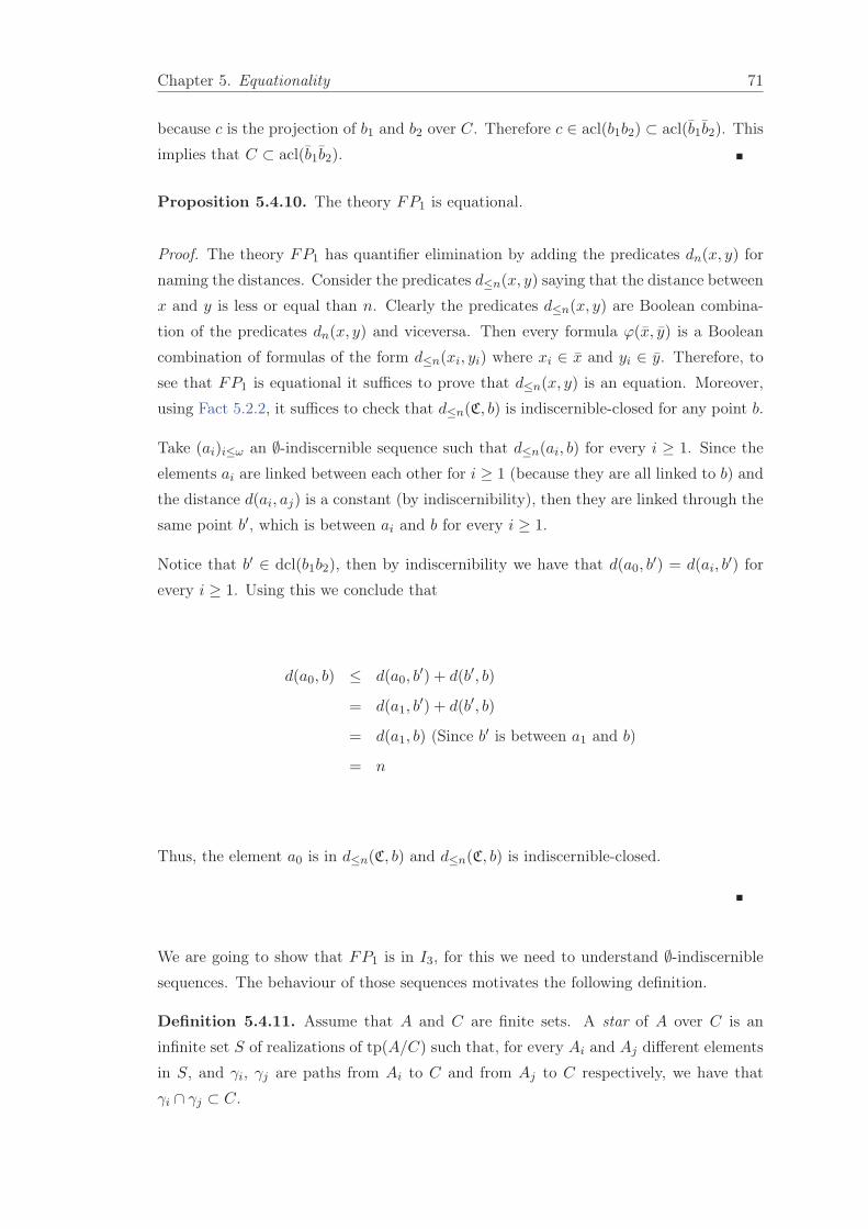
Chapter 5. Equationality 71
because c is the projection of b1 and b2 over C. Therefore c ∈ acl(b1b2) ⊂ acl(b1b2). This
implies that C ⊂ acl(b1b2).
Proposition 5.4.10. The theory FP1 is equational.
Proof. The theory FP1 has quantifier elimination by adding the predicates dn(x, y) for
naming the distances. Consider the predicates d≤n(x, y) saying that the distance between
x and y is less or equal than n. Clearly the predicates d≤n(x, y) are Boolean combina-
tion of the predicates dn(x, y) and viceversa. Then every formula ϕ(x, y) is a Boolean
combination of formulas of the form d≤n(xi, yi) where xi ∈ x and yi ∈ y. Therefore, to
see that FP1 is equational it suffices to prove that d≤n(x, y) is an equation. Moreover,
using Fact 5.2.2, it suffices to check that d≤n(C, b) is indiscernible-closed for any point b.
Take (ai)i≤ω an ∅-indiscernible sequence such that d≤n(ai, b) for every i ≥ 1. Since the
elements ai are linked between each other for i ≥ 1 (because they are all linked to b) and
the distance d(ai, aj) is a constant (by indiscernibility), then they are linked through the
same point b′, which is between ai and b for every i ≥ 1.
Notice that b′ ∈ dcl(b1b2), then by indiscernibility we have that d(a0, b′) = d(ai, b′) for
every i ≥ 1. Using this we conclude that
d(a0, b) ≤ d(a0, b′) + d(b′, b)
= d(a1, b′) + d(b′, b)
= d(a1, b) (Since b′ is between a1 and b)
= n
Thus, the element a0 is in d≤n(C, b) and d≤n(C, b) is indiscernible-closed.
We are going to show that FP1 is in I3, for this we need to understand ∅-indiscernible
sequences. The behaviour of those sequences motivates the following definition.
Definition 5.4.11. Assume that A and C are finite sets. A star of A over C is an
infinite set S of realizations of tp(A/C) such that, for every Ai and Aj different elements
in S, and γi, γj are paths from Ai to C and from Aj to C respectively, we have that
γi ∩ γj ⊂ C.

Chapter 5. Equationality 72
Remark 5.4.12. Assume S is a star over C and take Ai and Aj in S. If Ai is linked
to C then so is Aj , as the have the same type over C. Hence Ai and Aj are linked.
Moreover, any path from Ai to Aj must go through C. Then Ai |�CAj . By triviality of
forking, we have that S is an independent subset over C.
Our next goal is to characterize indiscernible sequences over ∅. Let us study first se-
quences of the form I = {ai}i<ω, where ai is connected for some (all) i < ω.
Lemma 5.4.13. Assume that a0 is connected. A infinite sequence I = (ai)i<ω is indis-
cernible over ∅ if and only if ai ≡ a0 for every i, and it has one of following mutually
exclusive forms:
1. For every i �= j, we have that ai is not linked with aj . In this case, the sequence I
is a star of a0 over c, where c is any element which is not linked to any ai.
2. For every i �= j, we have that ai is linked with aj and ai ∩ aj = ∅. In this case I is
a star of a0 over c, where c is a point in dcl(a0a1) such that d(c, ai) = n for a fixed
natural number n.
3. For every i �= j, we have that ai is linked with aj and ai ∩ aj = C �= ∅. In this
case, the sequence I is a star of a0 over C.
Proof. (⇒) Let I be an ∅-indiscernible sequence.
Case 1. Assume ai is not linked to aj . Take any c which is not linked to any ai, then
ai1 ...ainc ≡ aj1 ...ajnc, for any i1, ..., in and j1, ..., jn pairwise distinct. Thus I is a star
over c.
Case 2. Assume that ai is linked with aj and ai ∩ aj = ∅ for every i �= j. Then there is
a unique minimal path γi,j connecting ai and aj . Moreover the length of the paths γi,jis a constant n > 0. Now, take ai, aj and ak three different tuples of I and consider the
paths γi,j , γj,k and γi,k. As there are no cycles, the paths γi,j and γi,k must intersect the
path γj,k in the same point ci,j,k ,i.e. γi,j ∩ γi,k ∩ γj,k = {ci,j,k}. By indiscernibility of I,
we have that ci,j,k = ci′,j′,k′ = c for every i′, j′, k′. Moreover, again by indiscernibility,
the distance d(c, ai) is constant for every i. This implies that I is a star of a0 over c.
Case 3. Assume that ai is linked with aj and ai ∩ aj = C �= ∅ for every i �= j. By
indiscernibility, we have that I is a set of realizations of a0 over C. Moreover, any
path from ai to C is contained in ai, hence, if γi and γj go from ai to C and aj to C
respectively, then γi ∩ γj ⊂ ai ∩ aj = C. Thus, the sequence I is a star of a0 over C.
(⇐) Assume that I has one of these forms, then, by, Remark 5.4.4 it is ∅-indiscernible.
Chapter 5. Equationality 73
Lemma 5.4.14. Assume a is a connected tuple and let c be a single element connected
to a. Let us consider the sets:
D = {(a′, c′) | a′ |= tp(a/c) and c′ is in the path between c and proj(c/a)}.
E = {S |S is a star of a′ over c′, where (a′, c′) ∈ D}
Then we have that icl(tp(a/c)) =⋃
S∈E S.
Proof. Take p = tp(a/c). Notice that, for every S ∈ E , the set S ∩ p is infinite: take
S ∈ E a star of a′ over c′, where (a′, c′) ∈ D. Since a |�c′ c and tp(a/c′) is stationary,
then, for every a′′ ∈ S such that a′′ |�c′ c, we have that a ≡cc′ a′′. In particular a′′ |= p,
whenever a′′ ∈ S with a′′ |�c′ c. Notice also that there are infinitely many such a′′ in
S, therefore, if b ∈ S for some S ∈ E , then, by Lemma 5.4.13, we have that b is in an
indiscernible sequence, which has infinitely many elements in p. Thus b is in icl(p) and
icl(p) ⊃ ⋃S∈E S.
To check the other inclusion, let I = (ai)i<ω be an indiscernible sequence such that
ai ∈ p for every i ≥ 1. Then, according to the Lemma 5.4.13, we have that I is a star
of a0 over some set K. Note that proj(c/K) must be between a1 and c. Let us call this
element k and construct a new star S′ of a0 over k, such that the elements of S′ \ {a0}do not intersect dcl(S ∪ c), outside {k}. Take any element a′ ∈ S′ \ {a0}, since a0 ≡K a1
and a0 ≡k a′, we conclude that a1 ≡k a
′. Moreover c |�ka′. Therefore, by stationarity
a′ ≡ck a1. In particular a′ is in p, this implies that S′ is the star of a′ over k, where
(a′, k) ∈ D. Therefore icl(p) ⊂ ⋃S∈E S.
This description of icl(tp(a/c)) is useful as it helps to visualize why icl is idempotent:
since icl covers all the possible stars with infinitely many elements in p, then, by applying
icl twice, we do not get new stars. However, to make this intuition more precise, we need
to describe icl(p) in another way:
Definition 5.4.15. Let p = tp(a/c) and f be the function on q = tp(a/∅) defined as
follows:
If b ∈ p, then f(b) = proj(c/b).
If b /∈ p, then f(b) is the element that satisfies bf(b) ≡ af(a). (i.e. the position of f(b)
in b is the same of f(a) in a).

Chapter 5. Equationality 74
Lemma 5.4.16. Let n be the distance d(a, c) and consider the set
J = {a′ ≡ a | d(f(a′), c) = n− 2k, for some natural k}.
Then we have that icl(p) = J .
Proof. Using the previous lemma it suffices to show that
⋃S∈E
S = J
Let b ∈ ⋃S∈E S, then b is in the star of some element a′ ∈ p over some element c′ such
that c′ is between c and a′. Hence, either d(f(b), c) = n (and b ∈ J) , or f(b) is in the
path between c and c′. Therefore
d(f(b), c) = d(c′, c)− d(f(b), c′)
= n− d(f(b), c′)− d(f(b), c′).
Naming k = d(f(b), c′) we get that b ∈ J . Thus, we have⋃
S∈E S ⊂ J .
Assume now that b ≡ a and d(f(b), c) = n − 2k. Let γ(f(b), c′) be a path of length k
from f(b) to a new vertex c′ and such that γ ∩ dcl(b, c) = f(b). Now consider a star S
of b over c′. For all ai ∈ S with ai �= b we have that d(f(ai), c) = d(f(b, c)) + 2k = n.
Hence ai is in p and the element c′ is between ai and c. Therefore we conclude that
b ∈ ⋃S∈E S. Hence
⋃S∈E S ⊃ J .
With the last characterization we are now ready to prove the following:
Proposition 5.4.17. Let a be connected and C = dcl(cb(a/C)). Then we have icl2(tp(a/C)) =
icl(tp(a/C)) .
Proof. Let p = tp(a/C). We want to show that icl2(p) = icl(p).
Case 1: Assume C = ∅, then, if a ∈ icl(p), then there exists a sequence (ai)i≥1 of
realizations of p such that (ai)0≤i is ∅-indiscernible. In particular tp(a0/C) = tp(a0) =
tp(a1) = tp(a1/C). Therefore a0 |= p and icl(p) = p.
Case 2: Assume C has more than one element. Take any two elements c and c′ of C.
Then there are a and a′ in a such that c = proj(a/C), and c′ = proj(a′/C). As a is

Chapter 5. Equationality 75
connected and C is definable closed, then that the path from a to a′ passes through c
and c, in which case c and c′ are both in a. Since this is true for every c and c′ in C,
we conclude that C ⊂ a. On the other hand, any indiscernible sequence I with infinitely
many elements in p must be indiscernible over C. Therefore icl(p) = p.
Case 3: Assume that C = {c}.
By Lemma 5.4.16 we know that
icl(tp(a/c)) =⋃
a′∈Jtp(a′/c)
Therefore
icl 2(tp(a/c)) =⋃
a′∈Jicl(tp(a′/c)).
It remains to check that, if a′ ≡ a and d(f(a′), c) = n− 2k, then
icl(tp(a′/c)) ⊂ icl(tp(a/c)).
If b ∈ icl(tp(a′/c)), then there exist a tuple a′′ ∈ tp(a′/c) and an element c′′ between a′′
and c such that b is in a star of a′′ over c′′. Hence
d(f(b), c)) = d(c′′, c)− d(f(b), c′′)
= d(a′′, c)− d(f(b), c′′)− d(f(b), c′′)
= d(a′′, c)− 2d(f(b), c′′)
Since a′′ ∈ icl(p), we have d(a′′, c) = n − 2k for some k. Naming l = d(f(b, c′′)), we get
d(f(b), c)) = n− 2(k + l). Therefore b ∈ icl(tp(a/c)) and the conclusion follows.
Finally, we need to consider canonical types tp(a/C) where a is not connected.
Proposition 5.4.18. Let I = (aibi)i<ω be an indiscernible sequence where a0 is not
linked with b0. Then no ai is linked to bj with i �= j.
Proof. Recall that FP1 is stable, hence I is an indiscernible set. Assume there exists
i �= j such that ai is linked with bj . Then, by indiscernibility, the tuple ai is linked with
bj for every i �= j. In particular, we have the following path: a0 − b1 − a2 − b0, which is
a contradiction.

Chapter 5. Equationality 76
Proposition 5.4.19. Let p = tp(a/C) be a canonical type, then icl(p) = icl2(p).
Proof. We may assume that a = dcl(a), let a1...an be its connected components. We
may also assume that C = C1 ∪ ... ∪ Cn where Ci = cb(ai/C). Set pi = tp(ai/Ci).
We have that p = {b1...bn | bi |= pi and bi is not linked to bj for i �= j}. By the previous
proposition, it follows that
icl 2(p) = {b1...bn | bi ∈ icl 2(pi) and bi is not linked to bj for i �= j}.
Finally, as pi is the canonical type of a connected component we have icl(pi) = icl2(pi).
Hence icl(p) = icl2(p), which is the desired conclusion.
From the previous lemma we may conclude the main result.
Corollary 5.4.20. The theory FP1 is in I3.
Question 5.4.21. Let FPn be the theory of the n-dimensional free pseudospace. Is FPn
in In+2?
Question 5.4.22. If T is CM-trivial, then is it in I3?

Bibliography
[1] Adler H., Explanation of independence, Thesis dissertation, Albert Ludwigs
Freiburg University, 2005.
[2] Baudisch A., A new uncountably-categorical group, Transactions of the American
Mathematical Society 348, 3889-3940, 1996.
[3] Baudisch A., Pillay A., A free pseudospace, Journal of Symbolic Logic, 65(1),
443-460, 2000.
[4] Baudisch A., Martin-Pizarro A., Ziegler M., Ample hierarchy, Fundamenta Math-
ematicae, 224: 97-153, 2014.
[5] Baudisch A., Martin-Pizarro A., Ziegler M., A model theoretic study of right angle
buildings, Preprint, 2014.
[6] Baldwin J., A non-desarguesian projective plane, Transactions of the American
Mathematical Society 342(2), 695-711, 1994.
[7] Ben-Yaacov I., Pillay A., Vassiliev E., Lovely pairs of models, Annals of Pure and
Applied Logic. 122, 235-261, 2003.
[8] Berenstein A. Vassiliev E., On lovely pairs of geometric structures, Annals of pure
and applied logic. 161(7), 866-878, 2010.
[9] Berenstein A. Vassiliev E., Weakly one-based geometric structures, Journal of
symbolic logic, 77(2), 392-422, 2012.
[10] Berenstein A., Vassiliev E., Geometric structures with an independent subset,
(Preprint).
[11] Berenstein A., Carmona J., Vassiliev E., Structures of SU rank omega with an
independent dense subset, Preprint, 2014.
[12] Berenstein A. Kim J. Dense, codense predicates and NTP2, To be published in
Mathematical Logic Quaterly, 2014.
77
Chapter 5. Equationality 78
[13] Beyersdorff O., Comparing axiomatizations of free pseudospaces, Archive for
Mathematical Logic(48), 625-641. 2009.
[14] Berenstein A., Vassiliev E., On lovely pairs of geometric structures, Annals of
Pure and Applied Logic. 161(7),866-878, 2010.
[15] Carmona J., Forking geometry on geometric theories with an independent predic-
ate, Archive of Mathematical Logic 54, 247-255, 2015.
[16] Casanovas E.,Simple theories, Lectures notes in logic, Cambridge, 2001.
[17] Evans D., Ample dividing, The Journal of Symbolic Logic 68:1385-1402, 2003.
[18] Evans D., An introduction to ampleness, notes available at
http://www.uea.ac.uk/ h120/OxfordPGMT.pdf, 2015.
[19] Gagelman J.,Stability in geometric theories, Annals of Pure and Applied Logic
113:313-326, 2005.
[20] Grossberg R., Iovino J., Lessmann O., A primer on simple theories,
http://www.math.cmu.edu/ rami/simple.pdf.
[21] Hrushovski E., Pillay A., Weakly normal groups, In Logic Colloquium 85: 233-44,
1987.
[22] Hrushovski E., A new strongly minimal set, Annals of Pure and Applied Logic
62 (2):147-166, 1993.
[23] Hrushovski E., Srour G., A non-equational stable theory, Preprint.
[24] Hrushovski E., Simplicity and the Lascar group, preprint, 1998.
[25] Junker M., A note on equational theories, The Journal of Symbolic Logic 65(4):
1705-1712, 2000.
[26] Junker M., Lascar D., The indiscernible topology, a mock Zariski topology, Journal
of Mathematical Logic 1(1): 99-124, 2001.
[27] Nübling H., Reducts and expansions of stable and simple theories Thesis disser-
tation, University of East Anglia, 2004.
[28] Ohara A., Equations and equational theories ht-
tps://www.math.uwaterloo.ca/ rmoosa/ohara.pdf, 2011.
[29] Ould A., Tent K., Ampleness in the free group Preprint, 2012.

Chapter 5. Equationality 79
[30] Palacín D., Wagner F., Elimination of Hyperimaginaries and Stable Independence
in Simple CM-Trivial Theories. Notre Dame Journal of Formal Logic. 54. 541-551,
2013.
[31] Palacín D., Wagner F., Ample thoughts. The Journal of Symbolic Logic 78(2):489-
510, 2013.
[32] Palacín D., Forking in simple theories and CM-triviality. Ph.D thesis, 2012.
[33] Pillay A., Srour G., Closed Sets and Chain Conditions in Stable Theories, Journal
of Symbolic Logic 49(4): 1350-1362, 1984.
[34] Pillay A., The geometry of forking and groups of finite Morley rank, The Journal
of Symbolic Logic. 60(4):1251-1259, 1995.
[35] Pillay A. Geometric stability theory, Clarendon Press, 1996.
[36] Pillay A., A note on CM-triviality and the geometry of forking The Journal of
Symbolic Logic. 65(1):474-480, 2000.
[37] Sela Z., Free and hyperbolic groups are not equational, Preprint, 2014.
[38] Shelah S., Simple unstable theories, Annals of mathematical logic. 19:177-203,
1980.
[39] Sklinos R., On ampleness and pseudo-Anosov homeomorphisms in the free group,
Preprint, 2014.
[40] Srour G., The notion of independence in categories of algebraic structures, part
I: basic properties, Annals of Pure and Applied Logic, 38: 185-213, 1998.
[41] Srour G., The notion of independence in categories of algebraic structures, part
II: S-minimal extenstions, Annals of Pure and Applied Logic, 38: 185-213, 1998.
[42] Srour G., The notion of independence in categories of algebraic structures, part
II: equational classes, Annals of Pure and Applied Logic, 38: 185-213, 1998.
[43] Srour G., The independence relation in separably closed fields, The Journal of
Symbolic Logic 51(3): 715-725, 1986.
[44] Tent K., The free pseudospace is n-ample, but not (n + 1)-ample. Journal of
Symbolic Logic 79(2), 410âĂŞ428. 2014.
[45] Yoneda I., Some remarks on CM-triviality Journal of Mathematical Society. Ja-
pan. 61(2): 379-391. 2009.

Chapter 5. Equationality 80
[46] Ziegler M., Model Theory of Modules, Annals of Pure and Applied Logic, 26:
149-213, 1984.
[47] Zilber B., The structure of models of uncountably categorical theories, Proceedings
International Congress of Mathematicians 1983, Warszawa, PWN, North Holland
1, 359-368, 1984.
[48] Zilber B., Analytic and pseudoanalytic structures, Preprint, 2001.
[49] Zilber B., Zariski geometries. Geometry from the logicianâĂŹs point of view,
London Mathematical Society, 2010.