Expander Flows, Geometric Embeddings and Graph Partitioningarora/pubs/arvfull.pdfExpander ﬂows,...

Expander Flows, Geometric Embeddings and Graph Partitioning

SANJEEV ARORA

Princeton University

SATISH RAO

and

UMESH VAZIRANI

UC Berkeley

We give a O(√

log n)-approximation algorithm for the sparsest cut, edge expansion, balancedseparator, and graph conductance problems. This improves the O(log n)-approximation ofLeighton and Rao (1988). We use a well-known semidefinite relaxation with triangle inequalityconstraints. Central to our analysis is a geometric theorem about projections of point sets in d,whose proof makes essential use of a phenomenon called measure concentration.

We also describe an interesting and natural “approximate certificate” for a graph’s expansion,which involves embedding an n-node expander in it with appropriate dilation and congestion. Wecall this an expander flow.

Categories and Subject Descriptors: F.2.2 [Theory of Computation]: Analysis of Algorithms and Problem Complexity; G.2.2[Mathematics of Computing]: Discrete Mathematics and Graph Algorithms

General Terms: Algorithms,Theory

Additional Key Words and Phrases: Graph Partitioning,semidefinite programs,graph separa-tors,multicommodity flows,expansion,expanders

1. INTRODUCTION

Partitioning a graph into two (or more) large pieces while minimizing the size of the “interface” betweenthem is a fundamental combinatorial problem. Graph partitions or separators are central objects of studyin the theory of Markov chains, geometric embeddings and are a natural algorithmic primitive in numeroussettings, including clustering, divide and conquer approaches, PRAM emulation, VLSI layout, and packetrouting in distributed networks. Since finding optimal separators is NP-hard, one is forced to settle forapproximation algorithms (see Shmoys [1995]). Here we give new approximation algorithms for some of theimportant problems in this class.

Graph partitioning involves finding a cut with few crossing edges conditioned on or normalized by thesize of the smaller side of the cut. The problem can be made precise in different ways, giving rise toseveral related measures of the quality of the cut, depending on precisely how size is measured, such asconductance, expansion, normalized or sparsest cut. Precise definitions appear in Section 2. These measuresare approximation reducible within a constact factor (Leighton and Rao [1999]), are all NP-hard, and arisenaturally in different contexts.

A weak approximation for graph conductance follows from the connection —first discovered in the

Author’s address: S. Arora, Computer Science Department, Princeton University. www.cs.princeton.edu/∼arora. Workdone partly while visiting UC Berkeley (2001-2002) and the Institute for Advanced Study (2002-2003). Supported by Davidand Lucille Packard Fellowship, and NSF Grants CCR-0098180 and CCR-0205594 MSPA-MCS 0528414, CCF 0514993, ITR0205594, NSF CCF 0832797.S. Rao Computer Science Division, UC Berkeley. www.cs.berkeley.edu/∼satishr. Partially supported by NSF award CCR-0105533, CCF-0515304, CCF-0635357.U. Vazirani. Computer Science Division, UC Berkeley.www.cs.berkeley.edu/∼vazirani Partially supported by NSF ITR GrantCCR-0121555.A preliminary version of this paper appeared at ACM Symposium on Theory of Computing, 2004Permission to make digital/hard copy of all or part of this material without fee for personal or classroom use provided thatthe copies are not made or distributed for profit or commercial advantage, the ACM copyright/server notice, the title of thepublication, and its date appear, and notice is given that copying is by permission of the ACM, Inc. To copy otherwise, torepublish, to post on servers, or to redistribute to lists requires prior specific permission and/or a fee.c 20YY ACM 0004-5411/20YY/0100-0111 $5.00

Journal of the ACM, Vol. V, No. N, Month 20YY, Pages 111–0??.

112 · Sanjeev Arora et al.

context of Riemannian manifolds (Cheeger [1970])—between conductance and the eigenvalue gap of theLaplacian: 2Φ(G) ≥ λ ≥ Φ(G)2/2 (Alon and Milman [1985; Alon [1986; Jerrum and Sinclair [1989]). Theapproximation factor is 1/Φ(G), and hence Ω(n) in the worst case, and O(1) only if Φ(G) is a constant.This connection between eigenvalues and expansion has had enormous influence in a variety of fields (seee.g. Chung [1997]).

Leighton and Rao [1999] designed the first true approximation by giving O(log n)-approximations forsparsest cut and graph conductance and O(log n)-pseudo-approximations1 for c-balanced separa-tor. They used a linear programming relaxation of the problem based on multicommodity flow proposedin Shahrokhi and Matula [1990]. These ideas led to approximation algorithms for numerous other NP-hardproblems, see Shmoys [1995]. We note that the integrality gap of the LP is Ω(log n), and therefore improvingthe approximation factor necessitates new techniques.

In this paper, we give O(√

log n)-approximations for sparsest cut, edge expansion, and graph con-ductance and O(

√log n)-pseudo-approximation to c-balanced separator. As we describe below, our

techniques have also led to new approximation algorithms for several other problems, as well as a break-through in geometric embeddings.

The key idea underlying algorithms for graph partitioning is to spread out the vertices in some abstractspace while not stretching the edges too much. Finding a good graph partition is then accomplished bypartitioning this abstract space. In the eigenvalue approach, the vertices are mapped to points on the realline such that the average squared distance is constant, while the average squared distance between theendpoints of edges is minimized. Intuitively, snipping this line at a random point should cut few edges,thus yielding a good cut. In the linear programming approach, lengths are assigned to edges such that theaverage distance between pairs of vertices is fixed, while the average edge length is small. In this case, it canbe shown that a ball whose radius is drawn from a particular distribution defines a relatively balanced cutwith few expected crossing edges, thus yielding a sparse cut.

Note that by definition, the distances in the linear programming approach form a metric (i.e., satisfy thetriangle inequality) while in the eigenvalue approach they don’t. On the other hand, the latter approachworks with a geometric embedding of the graph, whereas there isn’t such an underlying geometry in theformer.

In this paper, we work with an approach that combines both geometry and the metric condition. Considermapping the vertices to points on the unit sphere in n such that the squared distances form a metric. Werefer to this as an 22-representation of the graph. We say that it is well-spread if the average squared distanceamong all vertex pairs is a fixed constant, say ρ. Define the value of such a representation to be the sum ofsquared distances between endpoints of edges. The value of the best representation is (up to a factor 4) alower bound on the capacity of the best c-balanced separator, where 4c(1− c) = ρ. The reason is that everyc-balanced cut in the graph corresponds to a 22 representation in a natural way: map each side of the cut toone of two antipodal points. The value of such a representation is clearly 4 times the cut capacity since theonly edges that contribute to the value are those that cross the cut, and each of them contributes 4. Theaverage squared distance among pairs of vertices is at least 4c(1− c).

Our approach starts by finding a well-spread representation of minimum value, which is possible in polyno-mial time using semidefinite programming. Of course, this minimum value representation will not in generalcorrespond to a cut. The crux of this paper is to extract a low-capacity balanced cut from this embedding.

The key to this is a new result (Theorem 1) about the geometric structure of well-spread 22-representations:they contain Ω(n) sized sets S and T that are well-separated, in the sense that every pair of points vi ∈ S

and vj ∈ T must be at least ∆ = Ω(1/√

log n) apart in 22 (squared Euclidean) distance. The set S can beused to find a good cut as follows: consider all points within some distance δ ∈ [0,∆] from S, where δ ischosen uniformly at random. The quality of this cut depends upon the value of representation. In particular,if we start with a representation of minimum value, the expected number of edges crossing such a cut mustbe small, since the length of a typical edge is short relative to ∆.

1For any fixed c < c the pseudo-approximation algorithm finds a c-balanced cut whose expansion is at most O(log n) timesexpansion of the best c-balanced cut.

Journal of the ACM, Vol. V, No. N, Month 20YY.

Expander flows, geometric embeddings, and graph partitioning · 113

Furthermore, the sets S and T can be constructed algorithmically by projecting the points on a randomline as follows (Section 3): for suitable constant c, the leftmost cn and rightmost cn points on the line areour first candidates for S and T . However, they can contain pairs of points vi ∈ S, vj ∈ T whose squareddistance is less than ∆, which we discard. The technically hard part in the analysis is to prove that nottoo many points get discarded. This delicate argument makes essential use of a phenomenon called measureconcentration, a cornerstone of modern convex geometry (see Ball [1997]).

The result on well-separated sets is tight for an n-vertex hypercube —specifically, its natural embeddingon the unit sphere in log n which defines an 22 metric— where measure concentration implies that any twolarge sets are within O(1/

√log n) distance. The hypercube example appears to be a serious obstacle to

improving the approximation factor for finding sparse cuts, since the optimal cuts of this graph (namely, thedimension cuts) elude all our rounding techniques. In fact, hypercube-like examples have been used to showthat this particular SDP approach has an integrality gap of Ω(log log n) (Devanur et al. [2006; Krauthgamerand Rabani [2006]).

Can our approximation ratio be improved over O(√

log n)? In Section 8 we formulate a sequence ofconditions that would imply improved approximations. Our theorem on well-separated sets is also importantin study of metric embeddings, which is further discussed below.

1.0.0.1 Expander flows:. While SDPs can be solved in polynomial time, the running times in practice arenot very good. Ideally, one desires a faster algorithm, preferably one using simple primitives like shortestpaths or single commodity flow. In this paper, we initiate such a combinatorial approach that realizes thesame approximation bounds as our SDP-based algorithms, but does not use SDPs. Though the resultingrunning times in this paper are actually inferior to the SDP-based approach, subsequent work has led toalgorithms that are significantly faster than the SDP-based approach.

We design our combinatorial algorithm using the notion of expander flows, which constitute an interestingand natural “certificate” of a graph’s expansion. Note that any algorithm that approximates edge expansionα = α(G) must implicitly certify that every cut has large expansion. One way to do this certificationis to embed2 a complete graph into the given graph with minimum congestion, say µ. (Determining µ

is a polynomial-time computation using linear programming.) Then it follows that every cut must haveexpansion at least n/µ. (See Section 7.) This is exactly the certificate used in the Leighton-Rao paper,where it is shown that congestion O(n log n/α(G)) suffices (and this amount of congestion is required onsome worst-case graphs). Thus embedding the complete graph suffices to certify that the expansion is atleast α(G)/ log n.

Our certificate can be seen as a generalization of this approach, whereby we embed not the completegraph but some flow that is an “expander” (a graph whose edge expansion is Ω(1)). We show that forevery graph there is an expander flow that certifies an expansion of Ω(α(G)/

√log n) (see Section 7). This

near-optimal embedding of an expander inside an arbitrary graph may be viewed as a purely structuralresult in graph theory. It is therefore interesting that this graph-theoretic result is proved using geometricarguments similar to the ones used to analyse our SDP-based algorithm. (There is a natural connectionbetween the two algorithms since expander flows can be viewed as a natural family of dual solutions to theabove-mentioned SDP, see Section 7.4.) In fact, the expander flows approach was the original starting pointof our work.

How does one efficiently compute an expander flow? The condition that the multicommodity flow is anexpander can be imposed by exponentially many linear constraints. For each cut, we have a constraintstating that the amount of flow across that cut is proportional to the number of vertices on the smaller sideof the cut. We use the Ellipsoid method to find the feasible flow. At each step we have to check if anyof these exponentially many constraints are violated. Using the fact that the eigenvalue approach gives aconstant factor approximation when the edge expansion is large, we can efficiently find violated constraints(to within constant approximation), and thus find an approximately feasible flow in polynomial time using

2Note that this notion of graph embedding has no connection in general to geometric embeddings of metric spaces, or geometricembeddings of graphs using semidefinite programming. It is somewhat confusing that all these notions of embeddings end upbeing relevant in this paper.



the Ellipsoid method. Arora, Hazan, and Kale [2004] used this framework to design an efficient O(n2) timeapproximation algorithm, thus matching the running time of the best implementations of the Leighton-Raoalgorithm. Their algorithm may be thought of as a primal-dual algorithm and proceeds by alternatelycomputing eigenvalues and solving min-cost multicommodity flows. Khandekar, Rao, and Vazirani [2006]use the expander flow approach to break the O(n2) multicommodity flow barrier and rigorously analysean algorithm that resembles some practially effective heuristics (Lang and Rao [2004]). The analysis givesa worse O(log2

n) approximation for sparsest cut but requires only O(log2n) invocations of a single

commodity maximum flow algorithm. Arora and Kale [2007] have improved this approximation factor toO(log n) with a different algorithm. Thus one has the counterintuitive result that an SDP-inspired algorithmruns faster than the older LP-inspired algorithm a la Leighton-Rao, while attaining the same approximationratio. Arora and Kale also initiate a new primal-dual and combinatorial approach to other SDP-basedapproximation algorithms.

Related prior and subsequent work.

Semidefinite programming and approximation algorithms: Semidefinite programs (SDPs) have nu-merous applications in optimization. They are solvable in polynomial time via the ellipsoid method (Grotschelet al. [1993]), and more efficient interior point methods are now known (Alizadeh [1995; Nesterov and Ne-mirovskii [1994]). In a seminal paper, Goemans and Williamson [1995] used SDPs to design good approx-imation algorithms for MAX-CUT and MAX-k-SAT. Researchers soon extended their techniques to otherproblems (Karger et al. [1998; Karloff and Zwick [1997; Goemans [1998]), but lately progress in this directionhad stalled. Especially in the context of minimization problems, the GW approach of analysing “randomhyperplane” rounding in an edge-by-edge fashion runs into well-known problems. By contrast, our theoremabout well separated sets in 22 spaces (and the “rounding” technique that follows from it) takes a moreglobal view of the metric space. It is the mathematical heart of our technique, just as the region-growingargument was the heart of the Leighton-Rao technique for analysing LPs.

Several papers have pushed this technique further, and developed closer analogs of the region-growingargument for SDPs using our main theorem. Using this they design new

√log n-approximation algorithms

for graph deletion problems such as 2cnf-deletion and min-uncut (Agarwal et al. [2005]), for min-lineararrangement (Charikar et al. [2006; Feige and Lee [2007]), and vertex separators (Feige et al. [2005a]).Similarly, min-vertex cover can now be approximated upto a factor 2−Ω(1/

√log n) (Karakostas [2005]),

an improvement over 2−Ω(log log n/ log n) achieved by prior algorithms. Also, a O(√

log n) approximationalgorithm for node cuts is given in Feige et al. [2005b].

However, we note that the Structure Theorem does not provide a blanket improvement for all the problemsfor which O(log n) algorithms were earlier designed using the Leighton-Rao technique. In particular, theintegrality gap of the SDP relaxation for min-multicut was shown to be Ω(log n) (Agarwal et al. [2005]),the same (upto a constant factor) as the integrality gap for the LP relaxation.

Analysis of random walks: The mixing time of a random walk on a graph is related to the first nonzeroeigenvalue of the Laplacian, and hence to the edge expansion. Of various techniques known for upperbounding the mixing time, most rely on lower bounding the conductance. Diaconis and Saloff-Coste [1993]describe a very general idea called the comparison technique, whereby the edge expansion of a graph islower bounded by embedding a known graph with known edge expansion into it. (The embedding need notbe efficiently constructible; existence suffices.) Sinclair [1992] suggested a similar technique and also notedthat the Leighton-Rao multicommodity flow can be viewed as a generalization of the Jerrum-Sinclair [1989]canonical path argument. Our results on expander flows imply that the comparison technique can be usedto always get to within O(

√log n) of the correct value of edge expansion.

Metric spaces and relaxations of the cut cone: The graph partitioning problem is closely related togeometric embeddings of metric spaces, as first pointed out by Linial, London and Rabinovich [1995] andAumann and Rabani [1998]. The cut cone is the cone of all cut semi-metrics, and is equivalent to the cone ofall 1 semi-metrics. Graph separation problems can often be viewed as the optimization of a linear functionover the cut cone (possibly with some additional constraints imposed). Thus optimization over the cutJournal of the ACM, Vol. V, No. N, Month 20YY.


cone is NP-hard. However, one could relax the problem and optimize over some other metric space, embedthis metric space in 1 (hopefully, with low distortion), and then derive an approximation algorithm. Thisapproach is surveyed in Shmoys’s survey [1995]. The integrality gap of the obvious generalization of our SDPfor nonuniform sparsest cut is exactly the same as as the worst-case distortion incurred in embeddingn-point 22 metrics into 1. A famous result of Bourgain shows that the distortion is at most O(log n), whichyields an O(log n)-approximation for nonuniform sparsest cut. Improving this has been a major openproblem.

The above connection shows that an α(n) approximation for conductance and other measures for graphpartitioning would follow from any general upper bound α(n) for the minimum distortion for embedding22 metrics into 1. Our result on well separated sets has recently been used Arora et al. [2008] to boundthis distortion by O(

√log n log log n), improving on Bourgain’s classical O(log n) bound that applies to any

metric. In fact, they give a stronger result: an embedding of 22 metrics into 2. Since any 2 metric is an1 metric, which in turn is an 22 metric, this also gives an embedding of 1 into 2 with the same distortion.This almost resolves a central problem in the area of metric embeddings, since any 2 embedding of thehypercube, regarded as an 1 metric, must suffer an Ω(

√log n) distortion (Enflo [1969]).

A key idea in these new developments is our above-mentioned main theorem about the existence of well-separated sets S, T in well-spread 22 metrics. This can be viewed as a weak “average case” embedding from22 into 1 whose distortion is O(

√log n). This is pointed out by Chawla, Gupta, and Racke [2005], who used

it together with the measured descent technique of Krauthgamer, Lee, Mendel, Naor [2005] to show thatn-point 22 metrics embed into 2 (and hence into 1) with distortion O(log3/4

n). Arora, Lee, and Naor [2008]improved this distortion to O(

√log n log log n), which is optimal up to log log n factor.

To see why our main theorem is relevant in embeddings, realize that usually the challenge in producingsuch an embedding is to ensure that the images of any two points from the original 22 metric are far enoughapart in the resulting 1 metric. This is accomplished in Arora et al. [2008] by considering dividing possibledistances into geometrically increasing intervals and generating coordinates at each distance scale. Our maintheorem is used to find a well-separated pair of sets, S and T , for each scale, and then to use “distance toS” as the value of the corresponding coordinate. Since each node in T is at least ∆/

√log n away from

every node in S, this ensures that a large number of ∆-separated pairs of nodes are far enough apart. TheO(√

log n log log n) bound on the distortion requires a clever accounting scheme across distance scales.We note that above developments showed that the integrality gap for nonuniform sparsest cut is

O(√

log n log log n). There was speculation that the integrality gap may even be O(1), but Khot and Vish-noi [2005] have shown it is at least (log log n) for some > 0.

2. DEFINITIONS AND RESULTS

We first define the problems considered in this paper; all are easily proved to be NP-hard (Leighton andRao [1999]). Given a graph G = (V,E), the goal in the uniform sparsest cut problem is to determinethe cut (S, S) (where |S| ≤

S without loss of generality) that minimizes

E(S, S)

|S|S

. (1)

Since |V | /2 ≤S

≤ |V |, up to a factor 2 computing the sparsest cut is the same as computing the edgeexpansion of the graph, namely,

α(G) = minS⊆V,|S|≤|V |/2

E(S, S)

|S| .

Since factors of 2 are inconsequential in this paper, we use the two problems interchangeably. Furthermore,we often shorten uniform sparsest cut to just sparsest cut. In another related problem, c-balanced-separator, the goal is to determine αc(G), the minimum edge expansion among all c-balanced cuts. (Acut (S, S) is c-balanced if both S, S have at least c |V | vertices.) In the graph conductance problem we



wish to determine

Φ(G) = minS⊆V,|E(S)|≤|E|/2

E(S, S)

|E(S)| , (2)

where E(S) denotes the multiset of edges incident to nodes in S (i.e., edges with both endpoints in S areincluded twice).

There are well-known interreducibilities among these problems for approximation. The edge expansion,α, of a graph is between n/2 and n times the optimal sparse cut value. The conductance problem can bereduced to the sparsest cut problem by replacing each node with a degree d with a clique on d nodes; anysparse cut in the transformed graph does not split cliques, and the sparsity of any cut (that does not splitcliques) in the transformed graph is within a constant factor of the conductance of the cut. The sparsest cutproblem can be reduced to the conductance problem by replacing each node with a large (say sized C = n2

size) clique. Again, small cuts don’t split cliques and a (clique non-splitting) cut of conductance Φ in thetransformed graph corresponds to the a cut in the original of sparsity Φ/C2. The reductions can be boundeddegree as well (Leighton and Rao [1999]).

As mentioned, all our algorithms depend upon a geometric representation of the graph.

Definition 1 (22-representation) An 22-representation of a graph is an assignment of a point (vector)to each node, say vi assigned to node i, such that for all i, j, k:

|vi − vj |2 + |vj − vk|2 ≥ |vi − vk|2 (triangle inequality) (3)

An 22-representation is called a unit-22 representation if all points lie on the unit sphere (or equivalently, allvectors have unit length.)

Remark 1 We mention two alternative descriptions of unit 22-representations which however will not playan explicit role in this paper. (i) Geometrically speaking, the above triangle inequality says that every vi andvk subtend a nonobtuse angle at vj . (ii) Every positive semidefinite n×n matrix has a Cholesky factorization,namely, a set of n vectors v1, v2, . . . , vn such that Mij = vi, vj. Thus a unit-22-representation for an n nodegraph can be alternatively viewed as a positive semidefinite n × n matrix M whose diagonal entries are 1and ∀i, j, k,Mij + Mjk −Mik ≤ 1.

We note that an 22-representation of a graph defines a so-called 22 metric on the vertices, where d(i, j) =|vi − vj |2 . We’ll now see how the geometry of 22 relates to the properties of cuts in a graph.

Every cut (S, S) gives rise to a natural unit-22-representation, namely, one that assigns some unit vectorv0 to every vertex in S and −v0 to every vertex in S.

Thus the following SDP is a relaxation for αc(G) (scaled by cn).

min14

i,j∈E

|vi − vj |2 (4)

∀i |vi|2 = 1 (5)

∀i, j, k |vi − vj |2 + |vj − vk|2 ≥ |vi − vk|2 (6)

i<j

|vi − vj |2 ≥ 4c(1− c)n2 (7)

This SDP motivates the following definition.

Definition 2 An 22-representation is c-spread if equation (7) holds.Journal of the ACM, Vol. V, No. N, Month 20YY.


Similarly the following is a relaxation for sparsest cut (up to scaling by n; see Section 6).

min

i,j∈E

|vi − vj |2 (8)

∀i, j, k |vi − vj |2 + |vj − vk|2 ≥ |vi − vk|2 (9)

i<j

|vi − vj |2 = 1 (10)

As we mentioned before the SDPs subsume both the eigenvalue approach and the Leighton-Rao ap-proach (Goemans [1998]). We show that the optimum value of the sparsest cut SDP is Ω(α(G)n/

√log n),

which shows that the integrality gap is O(√

log n).

2.1 Main theorem about 22-representations

In general, 22-representations are not well-understood3. This is not surprising since in d the representationcan have at most 2d distinct vectors (Danzer and Branko [1962]), so our three-dimensional intuition is oflimited use for graphs with more than 23 vertices. The technical core of our paper is a new theorem aboutunit 22-representations.

Definition 3 (∆-separated) If v1, v2, . . . , vn ∈ d, and ∆ ≥ 0, two disjoint sets of vectors S, T are∆-separated if for every vi ∈ S, vj ∈ T , |vi − vj |2 ≥ ∆.

Theorem 1 (Main)For every c > 0, there are c, b > 0 such that every c-spread unit-22-representation with n points contains ∆-separated subsets S, T of size cn, where ∆ = b/

√log n. Furthermore, there is a randomized polynomial-time

algorithm for finding these subsets S, T .

Remark 2 The value of ∆ in this theorem is best possible up to a constant factor, as demonstrated bythe natural embedding (scaled to give unit vectors) of the boolean hypercube −1, 1d. These vectors forma unit 22-representation, and the isoperimetric inequality for hypercubes shows that every two subsets ofΩ(n) vectors contain a pair of vectors — one from each subset — whose squared distance is O(1/

√log n)

(here n = 2d). Theorem 1 may thus be viewed as saying that every Ω(1)-spread unit 22-representation is“hypercube-like” with respect to the property mentioned in the theorem. Some may view this as evidencefor the conjecture that 22-representations are indeed like hypercubes (in particular, embed in 1 with lowdistortion). The recent results in (Chawla et al. [2005; Arora et al. [2008]), which were inspired by our paper,provide partial evidence for this belief.

2.1.1 Corollary to Main Theorem:√

log n-approximation. Let W =

i,j∈E14 |vi − vj |2 be the optimum

value for the SDP defined by equations (4)–(7). Since the vectors vi’s obtained from solving the SDP satisfythe hypothesis of Theorem 1, as an immediate corollary to the theorem we show how to produce a c-balancedcut of size O(W

√log n). This uses the region-growing argument of Leighton-Rao.

Corollary 2There is a randomized polynomial-time algorithm that finds with high probability a cut that is c-balanced,and has size O(W

√log n).

Proof: We use the algorithm of Theorem 1 to produce ∆-separated subsets S, T for ∆ = b/√

log n. Let V0

denote the vertices whose vectors are in S. Associate with each edge e = i, j a length we = 14 |vi − vj |2.

(Thus W =

e∈E we.) S and T are at least ∆ apart with respect to this distance. Let Vs denote all verticeswithin distance s of S. Now we produce a cut as follows: pick a random number r between 0 and ∆, andoutput the cut (Vr, V − Vr). Since S ⊆ Vr and T ⊆ V \ Vr, this is a c-balanced cut.

To bound the size of the cut, we denote by Er the set of edges leaving Vr. Each edge e = i, j onlycontributes to Er for r in the open interval (r1, r2), where r1 = d(i, V0) and r2 = d(j, V0). Triangle inequality

3As mentioned in the introduction, it has been conjectured that they are closely related to the better-understood 1 metrics.



Fig. 1. Vr is the set of nodes whose distance on the weighted graph to S is at most r. Set of edges leaving this set is Er.

implies that |r2 − r1| ≤ we. Hence

W =

e

we ≥ ∆

s=0|Es| .

Thus, the expected value of |Er| over the interval [0,∆] is at most W/∆. The algorithm thus produces acut of size at most 2W/∆ = O(W

√log n) with probability at least 1/2.

3. ∆ = Ω(LOG−2/3

N)-SEPARATED SETS

We now describe an algorithm that given a c-spread 22 representation finds ∆-separated sets of size Ω(n)for ∆ = Θ(1/ log2/3

n). Our correctness proof assumes a key lemma (Lemma 7) whose proof appears inSection 4. The algorithm will be improved in Section 5 to allow ∆ = Θ(1/

√log n).

The algorithm, set-find, is given a c-spread 22-representation. Constants c, σ > 0 are chosen appropri-ately depending on c.

set-find:Input: A c-spread unit-22 representation v1, v2, . . . , vn ∈ d.Parameters: Desired separation ∆, desired balance c, and projection gap, σ.Step 1: Project the points on a uniformly random line u passing through the origin, and computethe largest value m where half the points v, have v, u ≥ m.

Then, we specify that

Su = vi : vi, u ≥ m +σ√d,

Tu = vi : vi, u ≤ m.

If |Su| < 2cn, HALT.a

Step 2: Pick any vi ∈ Su, vj ∈ Tu such that |vi − vj |2 ≤ ∆, and delete vi from Su and vj fromTu. Repeat until no such vi, vj can be found and output the remaining sets S, T .

aWe note that we could have simply chosen m to be 0 rather than to be the median, but this version of theprocedure also applies for finding sparsest cuts.

Remark 3 The procedure set-find can be seen as a rounding procedure of sorts. It starts with a “fat”random hyperplane cut (cf. Goemans-Williamson [1995]) to identify the sets Su, Tu of vertices that projectfar apart. It then prunes these sets to find sets S, T .Journal of the ACM, Vol. V, No. N, Month 20YY.


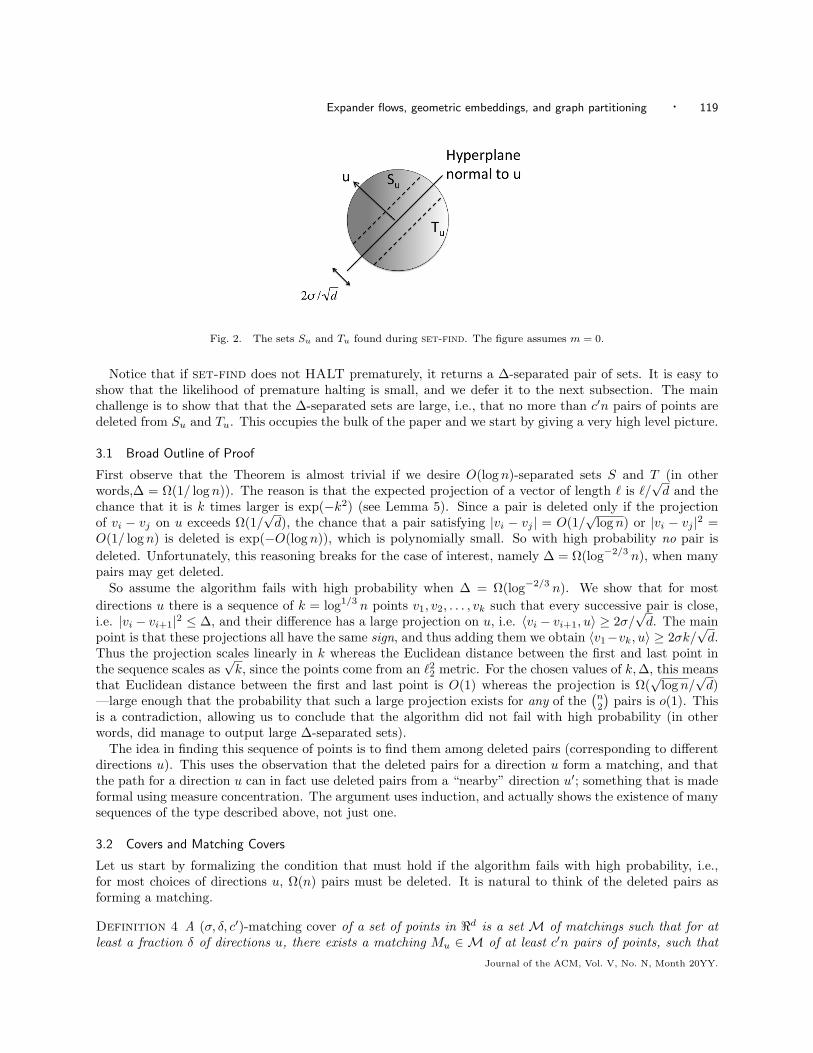
Fig. 2. The sets Su and Tu found during set-find. The figure assumes m = 0.

Notice that if set-find does not HALT prematurely, it returns a ∆-separated pair of sets. It is easy toshow that the likelihood of premature halting is small, and we defer it to the next subsection. The mainchallenge is to show that that the ∆-separated sets are large, i.e., that no more than cn pairs of points aredeleted from Su and Tu. This occupies the bulk of the paper and we start by giving a very high level picture.

3.1 Broad Outline of Proof

First observe that the Theorem is almost trivial if we desire O(log n)-separated sets S and T (in otherwords,∆ = Ω(1/ log n)). The reason is that the expected projection of a vector of length is /

√d and the

chance that it is k times larger is exp(−k2) (see Lemma 5). Since a pair is deleted only if the projectionof vi − vj on u exceeds Ω(1/

√d), the chance that a pair satisfying |vi − vj | = O(1/

√log n) or |vi − vj |2 =

O(1/ log n) is deleted is exp(−O(log n)), which is polynomially small. So with high probability no pair isdeleted. Unfortunately, this reasoning breaks for the case of interest, namely ∆ = Ω(log−2/3

n), when manypairs may get deleted.

So assume the algorithm fails with high probability when ∆ = Ω(log−2/3n). We show that for most

directions u there is a sequence of k = log1/3n points v1, v2, . . . , vk such that every successive pair is close,

i.e. |vi − vi+1|2 ≤ ∆, and their difference has a large projection on u, i.e. vi − vi+1, u ≥ 2σ/√

d. The mainpoint is that these projections all have the same sign, and thus adding them we obtain v1−vk, u ≥ 2σk/

√d.

Thus the projection scales linearly in k whereas the Euclidean distance between the first and last point inthe sequence scales as

√k, since the points come from an 22 metric. For the chosen values of k, ∆, this means

that Euclidean distance between the first and last point is O(1) whereas the projection is Ω(√

log n/√

d)—large enough that the probability that such a large projection exists for any of the

n2

pairs is o(1). This

is a contradiction, allowing us to conclude that the algorithm did not fail with high probability (in otherwords, did manage to output large ∆-separated sets).

The idea in finding this sequence of points is to find them among deleted pairs (corresponding to differentdirections u). This uses the observation that the deleted pairs for a direction u form a matching, and thatthe path for a direction u can in fact use deleted pairs from a “nearby” direction u; something that is madeformal using measure concentration. The argument uses induction, and actually shows the existence of manysequences of the type described above, not just one.

3.2 Covers and Matching Covers

Let us start by formalizing the condition that must hold if the algorithm fails with high probability, i.e.,for most choices of directions u, Ω(n) pairs must be deleted. It is natural to think of the deleted pairs asforming a matching.

Definition 4 A (σ, δ, c)-matching cover of a set of points in d is a set M of matchings such that for atleast a fraction δ of directions u, there exists a matching Mu ∈M of at least cn pairs of points, such that



each pair (vi, vj) ∈ Mu, satisfies

vi − vj , u ≥ 2σ/√

d.

The associated matching graph M is defined as the multigraph consisting of the union of all matchingsMu.

In the next section, we will show that step 1 succeeds with probability δ. This implies that if withprobability at least δ/2 the algorithm did not produce sufficiently large ∆-separated pair of sets, then withprobability at least δ/2 many pairs were deleted. Thus the following lemma is straightforward.Lemma 3If set-find fails with probability greater than 1− δ/2, on a unit c-spread 22-representation, then the set ofpoints has a (σ, δ/2, c)-matching cover.

The definition of (σ, δ, c)-matching cover M of a set of points suggests that for many directions there aremany disjoint pairs of points that have long projections. We will work with a related notion.

Definition 5 ((σ, δ)-uniform-matching-cover) A set of matchings M (σ, δ)-uniform-matching-coversa set of points V ⊆ d if for every unit vector u ∈ d, there is a matching Mu of V such that every(vi, vj) ∈ Mu satisfies |u, vi − vj| ≥ 2σ√

d, and for every i, µ(u : vi matched in Mu) ≥ δ. We refer to the set

of matchings M to be the matching cover of V .

Remark 4 The main difference from Definition 4 is that every point participates in Mu with constantprobability for a random direction u, whereas in Definition 4 this probability could be even 0.Lemma 4If a set of n vectors is (σ, γ,β)-matching covered by M, then they contain a subset X of Ω(nδ) vectors thatare (σ, δ)-uniformly matching covered by M, where δ = Ω(γβ).

Proof: Consider the multigraph consisting of the union of all matchings Mu’s as described in Definition 4.The average node is in Mu for at least γβ measure of directions. Remove all nodes that are matched on fewerthan γβ/2 measure of directions (and remove the corresponding matched edges from the Mu’s). Repeat.The aggregate measure of directions removed is at most γβn/2. Thus at least γβn/2 aggregate measure ondirections remains. This implies that there are at least γβn/4 nodes left, each matched in at least γβ/4measure of directions. This is the desired subset X.

To carry out our induction we need the following weaker notion of covering a set:

Definition 6 ((, δ)-cover) A set w1, w2, . . . , of vectors in d is an (, δ)-cover if every |wj | ≤ 1 andfor at least δ fraction of unit vectors u ∈ d, there exists a j such that u,wj ≥ . We refer to δ as thecovering probability and as the projection length of the cover.

A point v is (, δ)-covered by a set of points X if the set of vectors x− v|x ∈ X is an (, δ)-cover.

Remark 5 It is important to note that matching covers are substantially stronger notion than covers. Forexample the d-dimensional hypercube 1√

d−1, 1d is easily checked to be an (Ω(1),Ω(1))-cover (equivalently,

the origin is (Ω(1),Ω(1)) covered), even though it is only (Θ(1),Θ(1/√

d)) uniformly matching covered. Thisexample shows how a single outlier in a given direction can cover all other points, but this is not sufficientfor a matching cover.

3.3 Gaussian Behavior of Projections

Before we get to the main lemma and theorem, we introduce a basic fact about projections and use it toshow that step 1 of set-find succeeds with good probability.Lemma 5 (Gaussian behavior of projections)If v is a vector of length in d and u is a randomly chosen unit vector then

(1) for x ≤ 1, Pr[|v, u| ≤ x√d] ≤ 3x.



(2) for x ≤√

d/4, Pr[|v, u| ≥ x√d] ≤ e−x2/4.

Formally, to show that step 1 of set-find succeeds with good probability, we prove that the point setssatisfy conditions in the following definition.

Definition 7 A set of n points v1, . . . , vn ∈ d is (σ, γ, c)-projection separated if for at least γ fractionof the directions u, |Su| ≥ 2cn, where

Su = i : vi, u ≥ m + σ/√

d,

with m being the median value of vi, u.

Using part (i) of Lemma 5, we show that the points are sufficiently projection separated. Here, it isconvenient for the points to be on the surface of the unit sphere. Later, for approximating sparsest cutwe prove a similar statement without this condition.

Lemma 6For every positive c < 1/3, there are c, σ, δ > 0, such that every c-spread unit 22-representation is (σ, δ, c)-projection separated.

Proof: The c-spread condition states that

k,j |vk − vj |2 ≥ 4c(1−c)n2. Since |vk − vj | ≤ 2, we can concludethat

k,j |vk − vj | ≥ 2c(1 − c)n2. Applying Markov’s inequality, we can conclude that |vi − vj | ≥ c(1 − c)

for at least c(1− c)n2 pairs.For these pairs i, j, condition (1) of Lemma 5 implies that for a random u, that |vi, u− vj , u| is at least

c(1− c)/(9√

d) with probability at least 1/3.This implies that for σ = c(1 − c)/18, the expected number of pairs where |vi, u − vj , u| ≥ 2σ/

√d is

at least (2/3)c(1− c)n2. Each such pair must have at least one endpoint whose projection is at least σ/√

d

away from m; and each point can participate in at most n such pairs. Therefore the expected number ofpoints projected at least σ/

√d away from m is at least (2/3)c(1− c)n.

Applying Markov’s bound (and observing that the number of points is at most n) it follows that withprobability at least (1/3)c(1 − c) at least (1/3)c(1 − c)n points are projected at least σ/

√d away from m.

By symmetry, half the time a majority of these points are in Su. Thus the lemma follows with δ = c =(1/6)c(1− c). c = (1/6)c(1− c).

3.4 Main Lemma and Theorem

We are now ready to formally state a lemma about the existence, for most directions, of many pairs of pointswhose difference vi − vj has a large projection on this direction. (Sometimes we will say more briefly thatthe “pair has large projection.”) For each k, we inductively ensure that there is a large set of points whichparticipate as one endpoint of such a (large projection) pair for at least half the directions. This lemma (andits variants) is a central technical contribution of this paper.

Definition 8 Given a set of n points that is (σ, δ, c)-matching covered by M with associated matchinggraph M , we define v to be in the k-core, Sk, if v is (k σ

2√

d, 1/2)-covered by points which are within k hops

of v in the matching graph M .

Lemma 7For every set of n points v1, . . . , vn that is (σ, δ, c)-matching covered by M with associated matchinggraph M , there are positive constants a = a(δ, c) and b = b(δ, c) such that for every k ≥ 1:

(1) Either |Sk| ≥ akn.

(2) Or there is a pair (vi, vj) with distance at most k in the matching graph M , such that

|vi − vj | ≥ bσ/√

k.



We use this lemma below to show that set-find finds Ω(1/log1/3n)-separated sets. Later, we develop a

modified algorithm for finding Ω(1/√

log n)-separated sets.Subsequently, the aforementioned paper by J. R. Lee [2005] strengthened case 1 of the lemma to show the

existence of Sk of size at least |M |/2, and thus that case 2 meets the stronger condition that |vi − vj | ≥ gσ

for some constant g. This implies that set-find without any modification finds large Ω(1/√

log n)-separatedsets.

We can now prove the following theorem.

Theorem 8Set-find finds an ∆-separated set for a c-spread unit 22-representation v1, . . . , vn with constant probability

for some ∆ = Ω(1/ log2/3n).

Proof: Recall, that, by Lemma 3, if set-find fails, then the set of points is (σ, δ, c)-matching covered.Moreover, each pair (vi, vj) in any matching Mu for a direction u satisfies |vi − vj | ≤

√∆ and vi − vj , u ≥

2σ/√

d.

We will now apply Lemma 7 to show that such a matching covered set does not exist for ∆ = Θ(1/ log2/3n),

which means that set-find cannot fail for this ∆. Concretely, we show that neither case of the Lemmaholds for k = bσ/

√∆ where b is the constant defined in the Lemma.

Let us start by dispensing with Case 2. Since the metric is 22, a pair of points (vi, vj) within distance k inthe matching graph satisfies |vi − vj |2 ≤ k∆, and thus |vi − vj | ≤

√k∆. For our choice of k this is less than

bσ/√

k, so Case 2 does not happen.Case 1 requires that for at least 1

2 of the directions u there is a pair of vectors (vi, vj) such that |vi − vj | ≤√k∆ and where vi − vj , u ≥ kσ/2

√d.

For any fixed i, j, the probability that a randomly chosen direction satisfies this condition is at mostexp(−kσ2/16∆), which can be made smaller than 1/2n2 by choosing some ∆ = Ω(1/ log2/3

n) since k =Θ(log1/3

n). Therefore, by the union bound, the fraction of directions for which any pair i, j satisfies thiscondition is less than n2/2n2 ≤ 1/2. Thus Case 1 also cannot happen for this value of ∆.

This proves the theorem.

4. PROOF OF LEMMA 7

4.1 Measure concentration

We now introduce an important geometric property of covers. If a point is covered in a non-negligible fractionof directions, then it is also covered (with slightly smaller projection length) in almost all directions. Thisproperty follows from measure concentration which can be stated as follows.

Let Sd−1 denote the surface of the unit ball in d and let µ(·) denote the standard measure on it. For anyset of points A, we denote by Aγ the γ-neighborhood of A, namely, the set of all points that have distanceat most γ to some point in A.

Lemma 9 (Concentration of measure)If A ⊆ Sd−1 is measurable and γ >

2√

log(1/µ(A))+t√d

, where t > 0, then µ(Aγ) ≥ 1− exp(−t2/2).

Proof: P. Levy’s isoperimetric inequality (see Ball [1997]) states that µ(Aγ)/µ(A) is minimized for sphericalcaps4. The lemma now follows by a simple calculation using the standard formula for (d-1)-dimensionalvolume of spherical caps, which says that the cap of points whose distance is at least s/

√d from an equatorial

plane is exp(−s2/2).

The following lemma applies measure concentration to boost covering probability.

4Levy’s isoperimetric inequality is not trivial; see Schechtman [2003] for a sketch. However, results qualitatively the same —butwith worse constants— as Lemma 9 can be derived from the more elementary Brunn-Minkowski inequality; this “approximateisoperimetric inequality” of Ball, de Arias and Villa also appears in Schechtman [2003].



Lemma 10 (Boosting Lemma)Let v1, v2, . . . , be a finite set of vectors that is an (, δ)-cover, and |vi| ≤ . Then, for any γ >

√2 log(2/δ)+t√

d,

the vectors are also an (− γ, δ)-cover, where δ = 1− exp(−t2/2).

Proof: Let A denote the set of directions u for which there is an i such that u, vi ≥ . Since |vi − u|2 =1 + |vi|2 − 2u, vi we also have:

A = Sd−1 ∩

i

Ball

vi,

1 + |vi|2 − 2

,

which also shows that A is measurable. Also, µ(A) ≥ δ by hypothesis. Thus by Lemma 9, µ(Aγ) ≥1− exp(−t2/2).

We argue that for each direction u in Aγ , there is a vector vi in the (, δ) cover with vi, u ≥ − 2γ asfollows. Let u ∈ A, u ∈ Aγ ∩ Sd−1 be such that |u− u| ≤ γ.

We observe that u, vi = u, vi+ u − u, vi ≥ − γ, since |vi| ≤ .

Combined with the lower bound on µ(Aγ), we conclude that the set of directions u such that there is ani such that u, vi ≥ − 2γ has measure at least 1− exp(−t2/2).

4.2 Cover Composition

In this section, we give the construction that lies at the heart of the inductive step in the proof of Lemma 7.Let X ⊆ d be a point set that is uniform (, δ)-matching-covered, where Mu denotes as usual the matching

associated with direction u. Suppose Z ⊆ X consists of points in X that are (1, 1 − δ/2)-covered, and forvi ∈ Z let Zi denote points that cover vi.

The following lemma shows how to combine the cover and matching cover to produce a cover for a set Z

with projection length the sum of the projection lengths of the original covers.

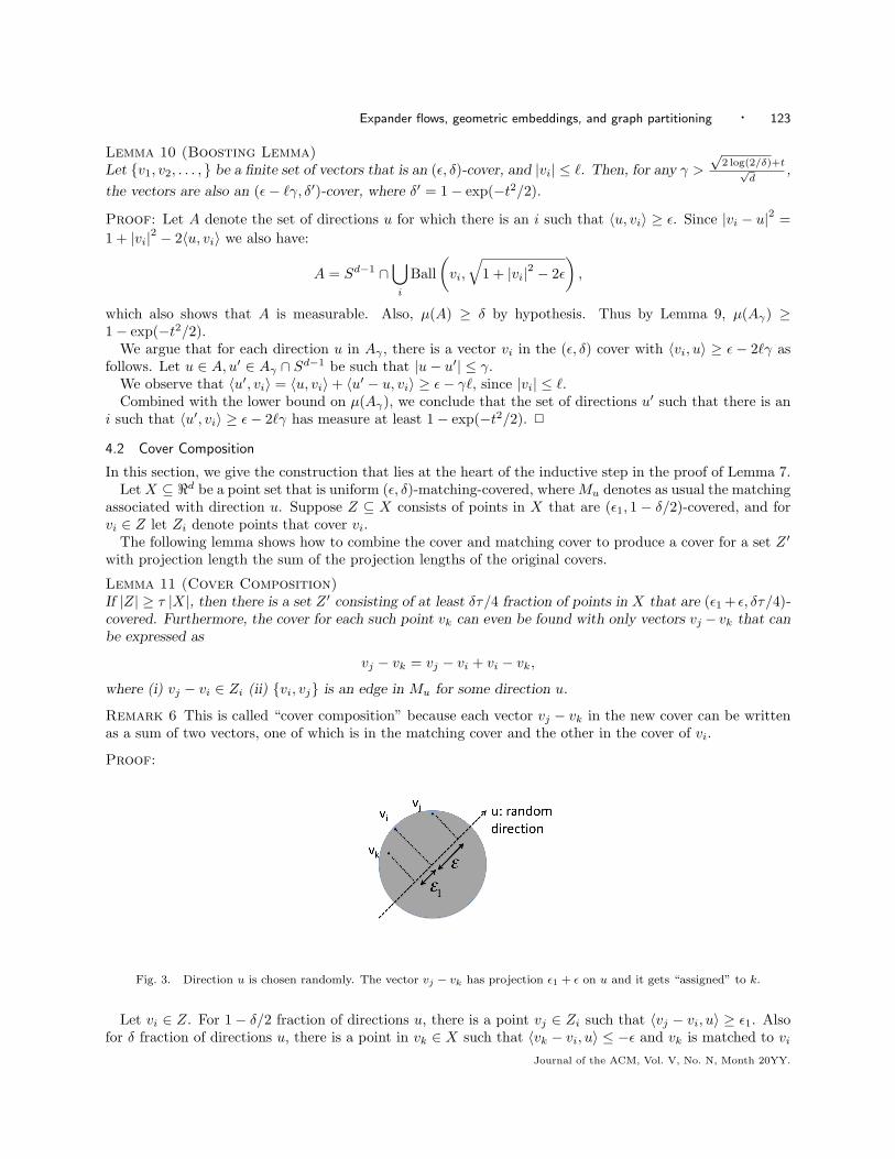
Lemma 11 (Cover Composition)If |Z| ≥ τ |X|, then there is a set Z consisting of at least δτ/4 fraction of points in X that are (1 + , δτ/4)-covered. Furthermore, the cover for each such point vk can even be found with only vectors vj − vk that canbe expressed as

vj − vk = vj − vi + vi − vk,

where (i) vj − vi ∈ Zi (ii) vi, vj is an edge in Mu for some direction u.

Remark 6 This is called “cover composition” because each vector vj − vk in the new cover can be writtenas a sum of two vectors, one of which is in the matching cover and the other in the cover of vi.

Proof:

Fig. 3. Direction u is chosen randomly. The vector vj − vk has projection 1 + on u and it gets “assigned” to k.

Let vi ∈ Z. For 1− δ/2 fraction of directions u, there is a point vj ∈ Zi such that vj − vi, u ≥ 1. Alsofor δ fraction of directions u, there is a point in vk ∈ X such that vk − vi, u ≤ − and vk is matched to vi



in the matching Mu. Thus for a δ/2 fraction of directions u, both events happen and thus the pair (vj , vk)satisfies vj − vk, u ≥ 1 + . Since vj ∈ Zi and vk ∈ X, we “assign” this vector vj − vk to point vk fordirection u, as a step towards building a cover centered at vk. Now we argue that for many vk’s, the vectorsassigned to it in this way form an (1 + , δ |Z| /2 |X|)-cover.

For each point vi ∈ Z, for δ/2 fraction of the directions u the process above assigns a vector to a pointin X for direction u according to the matching Mu. Thus on average for each direction u, at least δ|Z|/2vectors get assigned by the process. Thus, for a random point in X, the expected measure of directions forwhich the point is assigned a vector is at least δ|Z|/2 |X|.

Furthermore, at most one vector is assigned to any point for a given direction u (since the assignment isgoverned by the matching Mu). Therefore at least δ |Z| /4 |X| fraction of the points in X must be assigneda vector for δ |Z| /4 |X| = δτ/4 fraction of the directions.

We will define all such points of X to be the set Z and note that the size is at least δ |Z| /4 as required.

For the inductive proof of Lemma 7, it is useful to boost the covering probability of the cover obtained inLemma 11 back up to 1− δ/2. This is achieved by invoking the boosting lemma as follows.

Corollary 12If the vectors in the covers for Z have length at most

√

d

4

log 8τδ + 2

log 2

δ

then the (1 + , τδ/4)-covers for Z are also (1 + /2, 1− δ/2)-covers.

Proof:This follows from Lemma 10, since the loss in projection in this corollary is /2 which should be less than

γ where is the length of the vectors in the cover and γ is defined as in Lemma 10. Solving for yields theupper bound in the corollary.

Though the upper bound on the length in the hypothesis appears complicated, we only use the lemmawith = Θ(1/

√d) and constant δ. Thus, the upper bound on the length is Θ(1/

log(1/τ)). Furthermore,

1/τ will often be Θ(1).

4.3 Proof of Lemma 7

The proof of the lemma is carried out using Lemmas 10, and Corollary 12 in a simple induction.Before proving the lemma, let us restate a slight strengthening to make our induction go through.

Definition 9 Given a set of n points that is (σ, δ, c)-matching covered by M with associated matchinggraph M , we define v to be in the (k, ρ)-core, Sk,ρ, if v is (k σ

2√

d, 1− ρ)-covered by points which are within k

hops of v in the matching graph M .

Claim 13For constant δ, and every k ≥ 1,

(1) |Sk,δ/2| ≥ ( δ4 )k|X|

(2) or there is a pair (vi, vj) such that |vi − vj | = Ω(σ/√

k) and vi and vj are within k hops in the matchinggraph M .

Proof:Since the set of points is (σ, δ, c)-matching covered, Lemma 4 implies that there exists a (σ, δ)-uniform

matching cover M of a subset X of the point set. For k = 1, the claim follows by setting S1,δ/2 = X.Now we proceed by induction on k.Clearly if case 2 holds for k, then it also holds for k + 1. So assume that case 1 holds for k, i.e., Sk,δ/2

satisfies the conditions of case 1. Composing the covers of Sk,δ/2 with the matching cover M using Lemma 11Journal of the ACM, Vol. V, No. N, Month 20YY.


yields a cover for a set Z of size at least δ4 |Sk| with covering probability Θ(|Sk|/|X|), but with projection

length that is larger by = Ω(1/√

d). To finish the induction step the covering probability must be boostedto 1− δ/2 which by Lemma 10 decreases the projection length by

log Θ(|X|/|Sk|)/√

d = O(√

k/√

d) (11)

where upper-bounds the length of the vectors in the cover. If this decrease is less than /2, then thepoints in Z are (k/2 + /2, 1− δ/2)-covered and Sk+1,δ/2 is large as required in case 1. Otherwise we have/2 = Θ(σ/

√d) = O(

√k/√

d), which simplifies to ≥ gσ/√

k, for some constant g and thus case 2 holdsfor k + 1.

Remark 7 An essential aspect of this proof is that the k-length path (from Mk) pieces together pairs frommany different matchings Mu. Consider, for example, given a direction u and a matching Mu with projection on u, how we produce any pair of points with larger projection on u. Clearly, edges from the matching Mu

do not help with this. Instead, given any pair (x, y) ∈ Mu, we extend it with a pair (y, z) ∈ Mu for somedifferent direction u where (y, z) also has a large projection on u. The existence of such a pair (y, z) followsfrom the boosting lemma.

5. ACHIEVING ∆ = Ω(1/√

LOG N)

Theorem 1 requires ∆ = Ω(1/√

log n) whereas we proved above that set-find finds large ∆-separated setsfor ∆ = Ω(log−2/3

n). Now we would like to run set-find for ∆ = Ω(1/√

log n). The main problem inproving that set-find succeeds for larger ∆ is that our version of Lemma 7 is too weak. Before seeing howto remedy this it is useful to review how the proof of Theorem 1 constrains the different parameters andresults in a Θ(1/ log2/3

n) upper boundon ∆.

(1) In the proof of Lemma 7 we can continue to inductively assert case 1 (producing covered set Sk) ofClaim 13 as long as the right hand side of Equation (11) is less than σ/2

√d, i.e., as long as 2 1/k,

where bounds the lengths of the vectors.(2) By the triangle inequality, = O(

√k∆).

(3) Deriving the final contradiction in the proof of Theorem 8 requires that exp(−k/∆) 1/n2.

The limit on the vector lengths in item 1, combined with item 2, requires that k ≤ 1/∆1/2, and thus item3 constrains ∆ to be O(1/ log2/3

n).The improvement derives from addressing the limit on vector lengths in item 1, which arises from the

need to boost the covering probability for Sk (whose size decreases exponentially in k) from Θ(|Sk|/|X|) to1 − δ/2 as detailed in Equation (11). Thus, we would like to prevent the size of Sk from decreasing belowΩ(|X|). This will allow the induction to continue until the vectors have length Ω(1). To do so, we will usethe fact that any point close to a point which is (, δ)-covered is also (, δ)-covered where ≈ and δ ≈ δ.

This is quantified in Lemma 14.

Lemma 14 (Covering Close Points)Suppose v1, v2, . . . ∈ d form an (, δ)-cover for v0. Then, they also form an ( − ts√

d, δ − e−t2/4)-cover for

every v0 such that |v0 − v0| ≤ s.

Proof: If u is a random unit vector, Pru[u, v0 − v0 ≥ ts√d] ≤ e−t2/4.

Remark 8 Lemma 14 shows that (, δ) covers of a point are remarkably robust. In our context where wecan afford to lose Θ(1/

√d) in projection length, even a Θ(1)-neighborhood of that point is well covered.

Definition 10 (ζ-proximate graph) A graph G on a set of points v1, . . . , vn ∈ d is called ζ-proximate iffor each edge (vi, vj) in G, satisfies |vi − vj | ≤ ζ. A set of vertices S is non-magnifying if |S∪Γ(S)| < |V |/2,

where Γ(S) is the set of neighbors of S in G.Journal of the ACM, Vol. V, No. N, Month 20YY.


Notice that for any set S if the ζ-proximate graph is chosen to have edges between all pairs with distanceat most ζ that if T = V − S − Γ(S) then S, T is a ζ2-separated pair of sets. We will use ζ2 = ∆, thus if weever find a non-magnifying set S of size Ω(n) then we are done.

We prove a stronger version of Lemma 7 where case 2 only occurs when vectors have Ω(1) length byensuring in case 1 that the (k, δ/2)-core, Sk,δ/2, has size at least |X|/2.

The induction step in Lemma 11 now yields a set, which we denote by Sk+1, of cardinality δ|X|, which iscovered by X with constant covering probability and with projection length increased by Ω(1/

√d). If Sk+1

is a non-magnifying set in the ζ-proximate graph, we can halt (we have found a ζ-separated pair of sets forthe ζ-proximate graph above). Otherwise, Sk+1 can be augmented with Γ(Sk+1) to obtain a set T of size|X|/2 which by Lemma 14 is covered with projection length that is smaller by O(ζ/

√d) and is contained in

Sk+1,δ/2.Then, we boost the covering probability at a cost of reducing the projection length by O(/

√d) where is

the length of the covering vectors. Thus when ζ 1, we either increase the projection length by Ω(1/√

d)or is too large or we produce a non-magnifying set. This argument yields the following enhanced versionof Lemma 7:Lemma 15For every set of points X, that is (δ,σ)-uniform matching covered by M with associated matching graphM , and a ζ-proximate graph on the points for ζ ≤ ζ0(δ, c, σ), at least one of the following is true for everyk ≥ 1, where g = g(δ, c) is a positive constant.

(1) The (k, δ/2)-core, Sk,δ/2, has cardinality at least |X|/2(2) There is a pair (vi, vj) with distance at most k in the matching graph M , such that

|vi − vj | ≥ g.

(3) The set, Sk , is non-magnifying in the ζ-proximate graph for some k < k.

We can now prove Theorem 1. We use set-find with some parameter ∆ = Θ(1/√

log n). If it fails tofind a ∆-separated set the point set must have been (σ, δ, c)-matching covered where δ, c, and σ are Θ(1).We first apply Lemma 4 to obtain a (σ, δ)-uniform matching covered set X of size Ω(n). We then applyLemma 15 where the edges in the ζ-proximate graph consist of all pairs in X whose 22 distance is less thansome ζ2 = Θ(1/

√log n). If case 3 ever occurs, we can produce a pair of ζ-separated of size Ω(n). Otherwise,

we can continue the induction until k = Ω(√

log n) at which point we have a cover with projection lengthΘ(√

log n/√

d) consisting of vectors of O(1) length. As in our earlier proof, this contradicts the assumptionthat set-find failed.

Thus, either set-find gives a ∆-separated pair of large sets, or for some k, the ζ-neighborhood of Sk,Γ(Sk), is small and thus, Sk, V − Γ(Sk) forms a ζ-separated pair of large sets. Clearly, we can identify suchan Sk by a randomized algorithm that uses random sampling of directions to check whether a vertex is wellcovered.

This proves Theorem 1.

Remark 9 Lee’s direct proof that set-find [2005] produces Ω(1/√

log n)-separated sets relies on the fol-lowing clever idea: rather than terminating the induction with a non-magnifying set (in the ζ-proximategraph), he shows how to use the non-magnifying condition to bound the loss in covering probability. Themain observation is that after cover composition, the covering probability is actually |Sk|/|Γ(Sk)| rather thanour pessimistic bound of |Sk|/|X|. Thus by insisting on the invariant that |Γ(Sk)| = O(|Sk|), he ensuresthat the covering probability falls by only a constant factor, thus incurrring only a small boosting cost andallowing the induction to continue for k = Ω(1/∆) steps. Maintaining the invariant is easy since Sk canbe replaced by Γ(Sk) with small cost in projection length using Lemma 14. The point being that over thecourse of the induction this region growing (replacing Sk by Γ(Sk)) step only needs to be invoked O(log n)times.Journal of the ACM, Vol. V, No. N, Month 20YY.


6. O(√

LOG N) RATIO FOR SPARSEST CUT

Now we describe a rounding technique for the SDP in (8) – (10) that gives an O(√

log n)-approximationto sparsest cut. Note that our results on expander flows in Section 7 give an alternative O(

√log n)-

approximation algorithm.First we see in what sense the SDP in (8) –(10) is a relaxation for sparsest cut. For any cut (S, S)

consider a vector representation that places all nodes in S at one point of the sphere of squared radius(2 |S|

S)−1 and all nodes in |S| at the diametrically opposite point. It is easy to verify that this solution is

feasible and has valueE(S, S)

/ |S|S

.Since

S ∈ [n/2, n], we conclude that the optimal value of the SDP multiplied by n/2 is a lower bound

for sparsest cut.The next theorem implies that the integrality gap is O(

√log n).

Theorem 16There is a polynomial-time algorithm that, given a feasible SDP solution with value β, produces a cut (S, S)satisfying

E(S, S) = O(β |S|n

√log n).

The proof divides into two cases, one of which is similar to that of Theorem 1. The other case is dealtwith in the following Lemma.

Lemma 17For every choice of constants c, τ where c < 1, τ < 1/8 there is a polynomial-time algorithm for the following

task. Given any feasible SDP solution with β =

i,j∈E |vi − vj |2, and a node k such that the geometric

ball of squared-radius τ/n2 around vk contains at least cn vectors, the algorithm finds a cut (S, S) withexpansion at most O(βn/c).

Proof: Let d(i, j) denote |vi − vj |2, and when i, j is an edge e we write we for d(i, j). The weights we

turn the graph into a weighted graph.Let X be the subset of nodes that correspond to the vectors in the geometric ball of radius τ/n2 around

vk. The algorithm consists of doing a breadth-first search on the weighted graph starting from X. For s ≥ 0let Vs be the set of nodes whose distance from X is at most s, and let Es be the set of edges leaving Vs. Weidentify s for which the cut (Vs, Vs) has the lowest expansion, say αobs, and output this cut.

The expansion of the cut (Vs, Vs) is

|Es|min

|Vs| ,

Vs

.

Since |Vs| ≥ c ·Vs

, the expansion is at most

|Es|c ·

Vs

,

allowing us to conclude |Es| ≥ cαobs

Vs

for all s.To finish, we need to show that αobs = O(βn/c).Since

i<j d(i, j) = 1, the triangle inequality implies that each node m also satisfies:

i,j

d(i,m) + d(j,m) ≥ 1,

which implies

j

d(j,m) ≥ 1/2n. (12)

Separating terms corresponding to j ∈ X and j ∈ X in (12) and using cτ < 1/8 we obtain for the specialnode k:



j ∈X

d(j, k) ≥ 12n −

τn2 · cn ≥ 3

8n . (13)

The Lemma’s hypothesis also says

e∈E

we = β. (14)

As we noticed in the proof of Corollary 2, each edge e = i, j only contributes to Es for s in the openinterval (s1, s2), where s1 = d(i,X) and s2 = d(j,X). Triangle inequality implies that |s2 − s1| ≤ we.

Thus

β =

e∈E

we ≥

s>0|Es| ds ≥

s>0cαobs

Vs

ds.

Furthermore, we note that

s>0

Vs

ds =

i ∈X

d(i,X) ≥

i ∈X

(d(i, k)− τn2 ).

Thus, from equation (13) we have that

s>0

Vs

ds ≥ 38n − n · τ

n2>

14n

.

Combining the above inequalities, we obtain β ≥ cαobs/4n, or, in other words αobs = O(βn/c).

Now, in case the conditions of Lemma 17 does not hold, we run set-find.The following lemma ensures that for any point set that is c-spread and does not meet the conditions of

Lemma 17 that the procedure proceeds to Step 2 of set-find with a reasonable probability for a value of σ

that is Ω(1).

Lemma 18Given a c-spread set of points where no more than n/10 of them are contained in a ball of diameter 1/10,there is a σ = O(c) such that Step 1 of set-find does not HALT with probability at least Ω(1).

Proof:We begin with the following claim.

Claim 19For at least 1/20 of the directions, at least 1/20 of the pairs are separated by at least 1/90

√d in the projection.

Proof:Consider a vertex vi. The number of pairs vi, vj where |vi − vj | ≥ 1/10 is at least 9(n − 1)/10. Over all

pairs, the number is 9n(n− 1)/10. For unordered pairs, this is 9n(n− 1)/20.

For each such pair, the probability that vi and vj fall at least 1/90√

d apart is at least 1/3 from Lemma 5.Thus, the expected number of pairs that are separated by an interval of length 1/20

√d is at least 9n(n−1)/60.

Using the fact that the expected number can never be larger than n(n− 1)/2, we see that with probabilityat least 9/120 at least 9n(n− 1)/120 pairs are separated by at least 1/90

√d.

Notice that set-find with σ = 1/180 only HALTS in step 1 if more than 90% of the nodes are within1/180

√d of the median point. This does not occur with probability more than 19/20. Thus, Set-Find

succeeds with Ω(1) probability.

To finish, we observe that if the procedure fails in step 2, then the point set must be (σ, Θ(1),Θ(1))matching covered. We can then use Lemma 15 to produce a cut or to derive a contradiction as we didbefore.Journal of the ACM, Vol. V, No. N, Month 20YY.


7. EXPANDER FLOWS: APPROXIMATE CERTIFICATES OF EXPANSION

Deciding whether a given graph G has expansion at least α is coNP-complete (Blum et al. [1981]) and thushas no short certificate unless the polynomial hierarchy collapses. On the other hand, the value of the SDPused in the previous sections gives an “approximate” certificate of expansion. Jerrum and Sinclair [1989]and then Leighton and Rao [1999] previously showed how to use multicommodity flows to give “approxi-mate” certificates; this technique was then clarified by Sinclair [1992] and Diaconis and Saloff-Coste [1993].Their certificate was essentially an embedding of a complete graph into the underlying graph with minimalexpansion. This certificate could certify expansion to within a Θ(log n) factor.

The results of this section represent a continuation of that work but with a better certificate: for anygraph with α(G) = α we can exhibit a certificate to the effect that the expansion is at least Ω(α/

√log n).

Furthermore, this certificate can be computed in polynomial time. The certificate involves using multicom-modity flows to embed (weighted) expander graphs. The previous approaches were the same except that theexpander was limited to be the complete graph. In our approach, we can choose the expander which is theeasiest to embed in the underlying graph.

We remark that this view led to recent faster algorithms of Arora, Kale and Hazad [2004] for approximatingsparsest cuts. We note that this view essentially follows from SDP duality, in the sense that the certificatewe use is a feasible solution to the dual of the semi-definite program that we used in previous sections.

In this discussion it will be more convenient to look at weighted graphs. For a weighted graph G = (V,W )in which cij denotes the weight on edge i, j the sparsest cut is defined as

Φ(G) = minS⊆V :|S|≤n/2

i∈S,j∈S ci,j

|S|S

.

We similarly define α(G).A word on convention. Weighted graphs in this section will be symmetric, i.e., cij = cji for all node pairs

i, j. We call

j cij the degree of node i. We say that a weighted graph is d-regular if all degrees are exactlyd. We emphasize that d can be a fraction.

7.1 Multicommodity flows as graph embeddings

A multicommodity flow in an unweighted graph G = (V,E) is an assignment of a demand dij ≥ 0 to eachnode pair i, j such that we can route dij units of flow from i to j, and can do this simultaneously for all pairswhile satisfying capacity constraints. More formally, for each i, j and each path p ∈ Pij there exists fp ≥ 0such that

∀i, j ∈ V

p∈Pij

fp = dij (15)

∀e ∈ E

pe

fp ≤ 1. (16)

Note that every multicommodity flow in G can be viewed as an embedding of a weighted graph G =(V,E, dij) on the same vertex set such that the weight of edge i, j is dij . We assume the multicommodityflow is symmetric, i.e., dij = dji. The following inequality is immediate from definitions, since flows do notexceed edge capacities.

α(G) ≥ α(G) (17)

The following is one way to look at the Leighton-Rao result where Kn is the complete graph on n nodes.The embedding mentioned in the theorem is, by (17), a certificate showing that expansion is Ω(α/ log n).

Theorem 20 (Leighton-Rao [1999])If G is any n-node graph with α(G) = α, then it is possible to embed a multicommodity flow in it with eachfij = α/n log n (in other words, a scaled version of Kn).



Remark 10 The same theorem is usually stated using all fij = 1 (i.e., an unweighted copy of Kn) andthen bumping up the capacity of each edge of G to O(n log n/α). A similar restatement is possible for ourtheorem about expander flows (Theorem 24).

We note that the embedding of Theorem 20 can be found in polynomial time using a multicommodityflow computation, and that this embedding is a “certificate” via (17) that α(G) = Ω(α/ log n).

7.2 Expanders and Eigenvalues

Expanders can be defined in more than one way. Here, we first define the edge expansion ratio of a cut asthe ratio of the weight of edges across the cut to the total weighted degree of edges incident to the side thatis smaller with respect to total weighted degree. The edge expansion ratio of a graph is the minimum edgeexpansion ratio of any cut. Furthermore, a regular weighted graph, is a weighted graph where all the nodeshave the same weighted degree where the weighted degree of a node is the sum of the weights of the incidentedges. We note that the conductance is the edge expansion ratio divided by the total weighted degree of thebig side of the cut.

Definition 11 (Expanders) For any c > 0, a d-regular weighted graph (wij) is a β-expander if for everyset of nodes S, w(S, S) =

i∈S,j∈S wij is at least βd |S|. That is, its edge expansion ratio is at least β.

If a regular weighted graph is a β-expander, then the second eigenvalue of its Laplacian lies in the interval[β2/2, 2β] (see, for example, Alon [1986; Sinclair [1992].) In fact, we have the following algorithmic versionfrom Alon[1986] as well as Alon-Milman[1985].

Lemma 21There is a polynomial time algorithm that given a regular weighted graph with edge expansion ratio γ, findsa cut of weighted edge expansion ratio

√γ/2.

The next lemma extends the algorithm to output a balanced cut of small edge expansion ratio.

Lemma 22For any constant c > 0 there is a polynomial time algorithm that, given any regular weighted graph and anumber γ > 0 behaves as follows. If the graphs has a c-balanced cut of edge expansion ratio less than γ

then the algorithm outputs a c/2-balanced cut of edge expansion ratio 2√γ. If the graph does not have sucha cut, the algorithm finds a set of at least (1 − c/2)n nodes such that the induced subgraph (with deletededges replaced by self-loops) on them has edge expansion ratio at least 2γ.

Proof: First, we find a non-expanding cut in the weighted graph using the algorithm of Lemma 21 withthis value of γ. It either outputs a cut with edge expansion ratio at most √γ or else fails, in which case wehave verified that the graph has edge expansion ratio at least 2γ. In the former case, we delete the nodeson the small side of the cut and repeat on the remaining graph, where a self-loop is added to each nodewith weight equal to the removed degree for that node. We continue until the number of deleted nodes firstexceeds a c/2 fraction of the nodes. Now there are three cases to consider.

First, if the process deletes less than c/2 fraction of the vertices, then the remaining graph (which has atleast (1 − c/2)n vertices) has edge expansion ratio 2γ, and thus in the original graph every c-balanced cuthas edge expansion ratio at least γ.

Second, if the process deletes between c/2 and 1/2 of the nodes, then the union of the deleted sets givesa cut with edge expansion ratio at most √γ and we can therefore just output this union.

Finally, if the process deletes more than half the nodes in total then the final removed set had size greaterthan c/2 and has edge expansion ratio 2√γ, so the algorithm can output this final removed set.

Usually the word “expander” is reserved for the case when β > 0 is a fixed constant independent of thegraph size, in which case the second eigenvalue is bigger than some fixed positive constant. Thus an expanderfamily can be recognized in polynomial time by an eigenvalue computation, and this motivates our definitionof expander flows.Journal of the ACM, Vol. V, No. N, Month 20YY.


7.3 Expander flows

An expander flow is a multicommodity flow that is a β-expander for some constant β. Such flows can beused to certify the expansion of a graph.Lemma 23If a graph G contains a multicommodity flow (fij) that is d-regular and is a β-expander, then α(G) ≥ βd.

Proof: For every set S of nodes, the amount of flow leaving S is at least βd, and hence this is a lowerbound on the number of graph edges leaving S.

The previous Lemma is most useful if β is constant, in which case an eigenvalue computation can be usedto verify that the given flow is indeed an expander. Thus a d-regular expander flow may be viewed as acertificate that the expansion is Ω(d). The following Theorem says that such flows exist for d = α/

√log n in

every graph G satisfying α(G) = α. This is an interesting structural property of every graph, in the samespirit as Theorem 20. It also yields a certificate that α(G) = Ω(α/

√log n).

Theorem 24There is a constant β > 0 such that every n-vertex graph G contains a d-regular multicommodity flow in itthat is a β-expander, where d = α(G)/

√log n.

The theorem above is implied by the following algorithmic version of the theorem.Theorem 25There is a β0 > 0 and a polynomial-time algorithm that, given a graph G = (V,E) and a degree bound d,either finds a d-regular β0-expander flow in G or else finds a cut of expansion O(d

√log n).

The following lemma implies that to prove Theorem 25 it suffices to find a flow that expands on sets ofsize Ω(n) rather than all sets. It shows that given a flow that expands on large sets, one can either extendthis flow to expand on all sets or find a small cut.Lemma 26There is a polynomial time algorithm with the following property. Given a d-regular flow in a graph G =(V,E) where for all S ⊂ V , |S| ≥ cn, satisfies

i∈S,j∈S

fij ≥ βd|S|,

the algorithm either finds a cut of expansion O(d) or finds a 2d-regular Ω(β2) expander flow as long asβ = O(1).

Proof: We apply Lemma 22 to the weighted graph induced by the flow and obtain a subgraph B (with selfloops corresponding to the removed edges) which has (1− c/2)n ≥ 3n/4 nodes and has edge expansion ratioat least β2.

We now augment the given flow by embedding a single flowpath to each of the deleted nodes, A, as follows.We form a flow network, with each vertex in A being the source of d units of flow and each vertex in theremaining expander to be a possible sink of d units of flow, and place capacity one on each edge. We run amax-flow computation and either route d|A| units of flow or find a cut that cuts off some number say l ofthe sources from any remaining sink. In the latter case, the number of edges is at most dl, and thus the cuthas expansion at most d. Otherwise, the union of this flow and the previous d-regular flow can be embeddedwith constant congestion in G.

Furthermore, the resulting union is an Ω(β2) expander flow: Any cut S where at least 1/3 of S is in B

has edge expansion ratio in the induced flow graph of β2/3. Otherwise, at least 2/3 of S is in A, in whichcase the flow sends at least 2d|S|/3 units of flow into B at least d|S|/3 of which must go to nodes not in S.Thus, the cut has edge expansion ratio at least 1/3 which is Ω(β2) when β = O(1).

To make the final expander flow regular, we can add self-loops to augment the degree of each vertex to2d. This changes the edge expansion ratio by at most a factor of two.

Thus, to prove Theorem 25 it suffices to prove the following lemma.Journal of the ACM, Vol. V, No. N, Month 20YY.


Lemma 27For every β > 0 there is a γ = γ(β) > 0 and a polynomial time algorithm that, given a graph G = (V,E)and a degree bound d, either computes a d-regular flow (fij) satisfying for all S ⊂ V , |S| ≥ |V | /6

i∈S,j∈S

fij ≥ βd|S|,

or finds a cut of expansion γd√

log n.

Proof: The algorithm tries to find a feasible solution to the following linear program, where the goal is tofind a flow that expands on all large sets. Let Pij be the set of paths that go from i to j.

∀i

j

p∈Pij

fp ≤ d (18)

∀e

j

e∈p

fp ≤ 1 (19)

∀S ⊆ V, |V |/6 ≤ |S| ≤ |V |/2

i∈S,j∈S

p∈Pij

fp ≥ βd |S| . (20)

We note that if constraint (20) was enforced for all sets rather than just large sets, the resulting linearprogram would specify an expander flow. Note also that we only require the degree of the demand graph tobe at most d rather than exactly d. Any flow with max degree d can be trivially changed to a d-regular flowby adding self-loops at each node, which represent fictitious flows that use up no capacity.

Even though this linear program has exponentially many constraints, we can use the Ellipsoid algorithm tosolve it approximately in the following sense. Using the algorithm of Lemma 22 as an approximate separationoracle in the Ellipsoid algorithm, we can guarantee that if the LP is feasible for a certain β, then we canfind a solution that satisfies all constraints for a somewhat smaller value Ω(β2). Furthermore, if the LP isinfeasible for this value of β, then this algorithm finds a dual feasible solution of negative value to the closelyrelated linear program where the constraints (20) apply to sets of size down to |V |/6.

Thus the heart of the proof is to show how to produce a cut with expansion O(d√

log n) given such a dualfeasible solution. We will use ideas from our earlier SDP rounding algorithm, even though we are reasoningabout a linear program, not an SDP.

The dual has nonnegative variables zS for each S of size between |V |/6 and |V |/2 and the followingconstraints.

min

e

we + d

i

si − βd

S

zS |S|

e∈p

we + si + sj ≥

S:i∈S,j∈S

zS ∀i, j∀p ∈ Pij (21)

zS , we, si ≥ 0

We can assume that

S zS = 1 by rescaling, since scaling does not affect the sign of the dual objectivefunction.

Clearly, if the dual optimum is positive then the primal was feasible and hence an expander flow exists forthat value of β. To prove Lemma 27, we show that if β is such that the dual has a negative valued solutionthen we can use it to produce a cut of expansion O(d

√log n), where the constant in O(·) depends upon β.

Let us consider the we’s as weights on the edges. Then use the zS variables to define a well-spread 22-representation of the graph in M , where each of the M coordinates stands for a cut S where zS > 0.Each vertex x is mapped to a vector vx where the Sth coordinate is ±√zS depending on which side of S

it lies. Now |vi − vj |2 is up to a constant factor the same as the sum of zS ’s for all cuts (S, S) where i, j



are on opposite sides. This is the so-called “cut -metric,” and hence the vector representation is 22. (Thatis, |vi − vj |2 is a valid distance function satisfying triangle inequality.) Moreover, the sum of |vi − vj |2 overall pairs is Ω(n2). This is because zS is non-zero only for S’s that have size Ω(n), and thus the coordinatecorresponding to such a cut contributes Θ(zS) to the 22 distance for a constant fraction of pairs i, j. Hencethe typical pair of vertices is Ω(1) apart in 22 distance.

Thus the hypothesis of Lemma 28 (the next lemma below) is satisfied. Using the algorithm of that Lemmawe can either generate a cut of expansion O(d

√log n) or generate rn disjoint pairs with the following property.

For each pair i, j the length of the shortest path connecting them with respect to the weight function we haslength at most W/nd where W =

e we, and

|vi − vj |2 =

i∈S,j∈S

zS = ζ (22)

(i.e. the shortest path from i, j crosses a constant fraction of cuts). We show that the existence of suchpairs contradicts the assumption that the dual value was negative and hence the algorithm of Lemma 28must have generated a cut of expansion O(d

√log n).

Indeed, if such pairs exist then summing over the constraints (21) for them, we obtain

W

d+

i

si ≥ rζn,

or equivalently that

e

we + d

i

si − ζrdn ≥ 0.

Recall that the dual value is min

e we + d

i si − βd

S zS |S|. Observing that

S zS |S|[n/6, n] andchoosing a sufficiently small constant β, we make the dual value positive, and this is the desired contradiction.

Lemma 28For every c > 0 there are constants ζ = ζ(c) > 0, r = r(c) > 0, γ = γ(c) > 0 and a polynomial-timealgorithm with the following property. Given a graph G = (V,E), a number d > 0, an assignment ofnonnegative weights (we)e∈E to the edges, and a 22-representation v1, v2, . . . , vn where the distance betweenthe average vertex pair is at least c, the algorithm either outputs a cut of capacity γd

√log n or finds a list of

rn node pairs (with no vertex appearing in more than one pair) such that each pair (i, j) in the list satisfies:

length of shortest path from i to j in the weighted graph ≤ W

nd(23)

|vi − vj |2 ≥ ζ (24)

Proof: Our algorithm attempts first to find a small cut as follows:

(1) Project the vectors in the 22-representation onto a random direction u and identify two sets A and B

whose projections are ≥ m + σ/√

n and ≤ m− σ/√

n respectively on u where m is the median value ofthe projection of the vectors and σ is an appropriately small constant.

(2) It can be shown as we did in our analysis of sparsest cut that with good probability |A| , |B| are bothΩ(n). Let A be the smaller one. Solve the single commodity max flow problem in graph G where eachedge has capacity C = 1/kd with k = Θ(

√log n), and there is a unit capacity edge between the source

vertex and each node in A and a similar edge between the sink and each node in B. Use the algorithmto either compute a feasible flow of value |A| or output the minimum cut.

Notice, if the algorithm outputs a cut for any direction, this cut has expansion at most kd. This is becausethis cut must disconnect l vertices in A (resp., B) from the sink (resp., source), and the capacity of this cutmust be at most l. Hence the number of edges in the cut must be at most l/C ≤ lkd. Thus in this case weobtain a cut of expansion at most kd.



So suppose the algorithm finds a flow of value |A| for most directions u. We show how to apply Lemma 15to either find a cut of expansion O(d

√log n) or to produce a pair (i, j) satisfying conditions (23) and (24).

(We then indicate how the argument actually yields Ω(n) such pairs.) To apply that lemma, we must formmatching covers and define a proximity graph. Below, distance will refer to distance in the original weightedgraph with respect to the weights we’s on the edges, whereas geometric distance refers to squared Euclideandistance among the corresponding vectors.

The definition of the proximity graph is easy: there is an edge between each pair of vertices (i, j) whosedistance most W/kdn. If a pair of vertices is adjacent in the proximity graph and also has geometric distanceΩ(1) then such a pair satisfies (23) and (24) and we are done. So assume that every pair of adjacent verticesin the proximity graph have geometric distance at most ζ for an arbitrarily small ζ > 0.

Now we define the matching covers. For each direction u, use flow decomposition on the flow computedin step 2 above to obtain Ω(n) flowpaths. These flowpaths naturally define a pairing of nodes, since eachflowpath consists of a source edge to some node a ∈ A followed by a path to node b ∈ B followed by a sinkedge from b to the sink. Such a flowpath can be thought of as pairing a with b, and since each of these nodeshas a unique edge to the source/sink, this pairing is one-to-one (i.e., a partial matching). Now define thelength of the flowpath to be the sum of the edge weights in the path. The total length of all the flowpathsis at most CW since each edge can appear in at most C flowpaths. Thus, the average flowpath has lengthat most CW/ |A| = O(W/nkd). For a direction u, retain only those pairs in the partial matching where theflowpath length is at most twice the average length. This yields a matching with Ω(n) pairs where the pairsare within O(W/nkd) distance.

Now we have the matching covered point set and the ζ-proximate graph as required by the hypothesis ofLemma 15. Let k = Θ(

√log n) be some large enough multiple of

√log n, such that as in our earlier proofs,

it is impossible for the set Sk in the lemma statement to be nonempty (simply because no element can beprojection covered with such large projections). Then either case 2 or 3 of Lemma 15 must hold for k.

If case 3 of Lemma 15 holds then we obtain a non-magnifying set S of size Ω(n) in the ζ-proximategraph. Hence the set of nodes with no direct edges to S in the proximate graph (i.e. nodes whose distanceto S in the original graph is at most W/kdn) have size Ω(n). Now we choose a random positive δ in theinterval [0, W/kdn] and output the set containing all nodes whose distance (with respect to the weights we’son the edges) to the closest point of S is at most δ. The expected number of edges in this cut is at mostW/(W/kdn) = kdn. As already noted, each side of the cut has Ω(n) nodes. Thus the expected expansion ofthe cut is O(kd).

Case 2 of Lemma 15 yields a pair of vertices i, j whose geometric distance is Ω(1) and that are k matchinghops away, which corresponds to distance kW/kdn = O(W/dn) in the original graph since both k and k

are Θ(√

log n).Thus in every case we obtain a pair (i, j) satisfying (23) and (24). Now we note that the argument can

be repeated Ω(n) times to generate more such pairs. Indeed, deleting this pair leaves a set of vertices thatremains matching covered for slightly worse parameters; it removes at most 2 pairs from the Θ(n) pairs ineach matching. Thus, either the process can be repeated Θ(n) times to yield Θ(n) pairs or it fails at somepoint and produces a cut in some iteration as stated in the lemma.

We note that as before the analysis can be simplified using Lee’s techniques [2005]. In particular, cuts canbe produced using only a projection based procedure as is the case for finding sparse cuts using semidefiniteprogramming.

7.4 Expander flows as dual solutions

Now we show that expander flows are actually a natural family of dual solutions to the SDP for sparsestcut. Denote by OPT (W ) the value of the simplest SDP relaxation (with no triangle inequality) of thisproblem: find vectors v1, v2, . . . , vn ∈ n so as to:Journal of the ACM, Vol. V, No. N, Month 20YY.


min

i,j

ci,j |vi − vj |2 (25)

i =j

|vi − vj |2 = 1 (26)

Let OPT∆(W ) denote the value of the relaxation when we also impose the triangle inequality constraints.Now we relate OPT (·) and OPT∆(·).

Recall from our discussion of expander flows that a multicommodity flow in G can be viewed as anembedding of the demand graph D = (dij). We will show that such a flow is a dual solution to the SDPrelaxation with triangle inequality (we have learnt that this observation was known to others, includingSudan and Williamson).

Lemma 29 (Flows as dual solutions)If a demand graph D = (dij) can be embedded in G = (V,W ) then

OPT∆(W ) ≥ OPT (D).

Remark 11 Of course, when D is an expander, then the value OPT (D) is (upto scaling) essentially thesame as the eigenvalue bound for sparsest cut.

To prove the lemma we need to write the duals. Let us do this for the simple SDP, first rewriting it using xij

and zij to replace |vi − vj |2 and < vi, vj > respectively. We use diag(ai) to denote the n× n matrix whichhas a1, a2, . . . , an on the diagonal and 0 everywhere else.

PRIMAL DUAL (27)

min

i,j

cijxij max z (28)

i,j

xij = 1 z + sij = cij ∀i, j (29)

∀i, j xij + 2zij − zii − zjj = 0 sij unrestricted (30)

(zij) is psd diag(

j =i

sij)− (sij)i =j is psd (31)

Now we consider the SDP with triangle inequality. The usual formulation is to write for each triple i, j, k

an additional constraint: xij + xjk ≥ xik . We use an equivalent but more complicated formulation: if Pij

denotes the set of paths from i to j in the complete graph on n vertices, then

∀i, j, ∀p ∈ Pij ,

(u,v)∈p

xuv ≥ xij (32)

Now let us write the primal and the dual.Journal of the ACM, Vol. V, No. N, Month 20YY.


PRIMAL DUAL

min

i,j

cijxij max z

i,j

xij = 1 z + sij −

p∈Pij

fp + tij = cij ∀i, j (33)

∀i, j xij + 2zij − zii − zjj = 0 sij unrestricted (34)

∀i, j, ∀p ∈ Pij ,

(u,v)∈p

xuv ≥ xij (35)

(zij) is psd diag(

j =i

sij)− (sij)i =j is psd (36)

Here tij is a shorthand for

pi,j fp.Now let D be the demand graph of any multicommodity flow that can be embedded in G. A flow is an

assignment of nonnegative values to fp’s such that tij ≤ cij (indeed, the only nonzero fp’s are for p that areactually paths in G). Fixing these values of fp’s, finding the best values to z and the sij ’s is nothing butthe same as finding OPT (W ) where W is the weighted graph in which W

ij is cij − tij + Dij , where Dij isthe total flow from i to j, namely

p∈Pij

fp. Of course, since tij ≤ cij , this is lower bounded by OPT (D)where D is the demand graph of the flow. Thus the lemma is proved.

8. THE OPEN QUESTIONS

Currently it is completely plausible that our techniques can be strengthened to achieve an approximationratio much better than

√log n for uniform sparsest cut. Originally it was suggested in Goemans [1998]

that the SDP with triangle inequality has an integrality gap of O(1) but Khot and Vishnoi [2005] showedthat the gap is Ω(log log1/6

n), which was improved to Ω(log log n) by Krauthgamer and Rabani [2006] forthe nonuniform sparsest cut. Recently, Devanur et al. [2006] showed that the Ω(log log n) gap holds even forthe uniform version. As noted earlier, the example of the boolean hypercube shows that our main theorem(Theorem 1) about the existence of large ∆-separated subsets cannot be improved, so some newer idea seemsnecessary.

Below we provide a suggested roadmap for attacking these questions. We three questions. All concern anyconstant degree graph G = (V,E) and any unit-22- representation v1, v2, . . . , vn, that is c-spread for someconstant c.

Is there a function s(n) = o(√

log n) such that:

Question 1:. there is always an edge i, j ∈ E such that |vi − vj |2 = Ω(α/s(n))?

Question 2:. there are pairs of vertices i, j such that dG(i, j) = O(s(n)/α) and |vi − vj |2 = Ω(1)?Question 3:. Version of Question 2 whereby for some τ > 0, an arbitrary set of τ fraction of nodes are

forbidden from being chosen as i, j and nevertheless these i, j exist.

Earlier in the paper we proved that the answer to these questions is Yes if s(n) = O(√

log n). The authorscould not agree on a guess as to whether or not the answer is Yes to any of these questions for an s(n) thatgrows slower.

Now we summarise, without detailed proofs, the implications if the answers to these questions are Yes.

Lemma 30(1) If the integrality gap of the SDP is O(s(n)) then the answer to Question 1 is Yes.

(2) A Yes answer to Question 2 suffices to prove that the integrality gap is O(s(n)).(3) A Yes answer to Question 3 implies the existence of expander flows in graphs that certify expansion of

α/s(n). Namely, Theorem 24 is true with d = α/s(n).Journal of the ACM, Vol. V, No. N, Month 20YY.


(4) A Yes answer to Question 2 implies YES for question 1.

Proof:

(1) If the integrality gap of the SDP is O(s(n)) then the value of the objective is Ω(αn/s(n)) and hence atleast one edge has value Ω(α/s(n)).

(2) Uses a modification of our original proof that the integrality gap is O(√

log n).(3) Question 3 is a stronger version of statements proved earlier. One can mimic the proof of Theorem 24

(specifically, the last few lines of Lemma 27) using this stronger version.

8.1 Bringing the Question “down” to 1

Before explaining the title of this section we first recall the connection between cut problems and em-beddings into 1. A unit 22-representation v1, v2, . . . , vn of a graph is said to be 1 if there is a set ofvectors u1, u2, . . . , un such that |vi − vj |2 = |ui − uj |1. We say that it is 1 upto distortion c if |ui − uj |1 ≤|vi − vj |2 ≤ c · |ui − uj |1. The importance of embeddings to cut problems arises from the following equivalentcharacterization.Lemma 31 (well-known)A unit 22-representation v1, v2, . . . , vn is 1 iff there is a αS ≥ 0 associated with each cut (S, S) such that

|vi − vj |2 =

S

αSdS(i, j), (37)

where dS(i, j) = 0 if i, j are on the same side of the cut and 4 otherwise. (In other words, 1 representationscorrespond exactly to the cut cone.)

Proof: One direction is trivial from convexity since every cut metric is 1.For a proof of the other direction see Shmoys’ survey [1995] or Matousek’s book [2002].

Thus minimization over 1 metrics is exactly equivalent to minimizing over cuts (and thus NP-hard).Goemans and Linial independently conjectured that every 22-representation is 1 upto a distortion factorO(1). If true, this would have implied an integrality gap of O(1) for nonuniform sparsest cut, butrecently Khot and Vishnoi showed that distortion (log log n) is necessary. However the best upper boundon the distortion is O(

√log n log log n), so a large gap remains.

One may reasonably question whether it makes much sense to focus attention exclusively on 22 metricswhen these metrics merely happen to capture the properties of one family of SDPs. Shouldn’t one expendmore effort in identifying stronger SDP relaxations by specifying more constraints than the triangle inequal-ity? After all, procedures such as Lovasz-Schrijver [1991] give us an infinite hierarchy of progressively tighterSDP relaxations to choose from. (The triangle inequality constraint is implied already in the relaxation atthe third level of this hierarchy.)

Now we point out that at least in context of our Questions, adding other constraints (in addition to thetriangle inequality) to the SDP may not help. We bring “down” the Questions to 1 so that it suffices toprove them for 1 metrics. Thus although adding other constraints could conceivably give a class of metricsthat is a proper subset of 22, proving our conjectures for that other class of metrics will not be any easier,since that class of metrics (being a relaxation of cut metrics) would always contain 1.

[Question 4:] If the unit-22-representation is actually 1, then there is a vertex pair i, j such that dG(i, j) =O(s(n)/α) and |vi − vj |2 = Ω(1).

Lemma 32Questions 2 and 4 are equivalent.

Proof: Yes to Question 2 ⇒ Yes to Question 4: Since 1 metrics are a subcase of 22 metrics, Question 4 istrivially a subcase of Question 2.



Yes to Question 4 ⇒ Yes to Question 2: Given any unit-22-representation v1, v2, . . . , vn of the graph,consider the uniform distribution on all hyperplane cuts (a la [GW]). Represent this distribution usingLemma 31 by an 22-representation that is 1, namely, a set of unit vectors u1, u2, . . . , un where

|ui − uj |2 = Pr[i, j are separated in hyperplane cut produced using v1, . . . , vn].

Let i, j be the pair of nodes in G whose existence follows if Question 4 has a Yes answer. Namely, |ui − uj |2 =Ω(1). Then these also suffice for Question 2 since if

Pr[i, j are separated in hyperplane cut on v1, . . . , vn] = Ω(1),

then |vi − vj |2 = Ω(1) also.

Remark 12 We can make a robust form of Question 4 whereby the pair exists even if we forbid τn nodesfrom playing the role of i, j. Giving a Yes answer to that question is equivalent to showing that expanderflows can be used to certify an expansion of α/s(n).

9. CONCLUSIONS

In the four years since the initial distribution of this paper, the geometric techniques introduced here havefound many uses in designing other SDP-based approximation algorithms as well as resolving open questionsin metric space embeddings. We see several promising avenues of research in the near future.

First, there appears to be plenty of scope to use more sophisticated geometric arguments in analysing SDPs.Procedures such as Lovasz-Schrijver [1991] or Sherali-Adams [1990] in principle give an infinite family of SDPrelaxations that have thus far resisted all attempts at analysis but may have low integrality gaps. Since thetriangle inequality constraints are obtained trivially in these frameworks, perhaps our analysis of the triangleinequality constraints gives a hint how to analyse more complicated SDPs.

Second, as already mentioned even the SDPs with triangle inequality are not fully understood as yet: thereis a big gap between the lower bounds and upperbounds known on the integrality gap. A similar observationholds for questions about geometric embeddings such as the distortion required to embed 22 metrics into 1.

Finally, there is a need to design efficient approximation algorithms, since solving SDPs is fairly inefficient(though polynomial time). Solving the SDP of (4)–(7) takes about n4.5 time for an n-node graph usinginterior point methods. As mentioned, a more efficient O(n2)-time algorithm is now known (Arora et al.[2004]) that uses expander flows. Recently a more general primal-dual framework was invented (Arora andKale [2007]) for replacing SDPs with faster approximation algorithms for problems other than sparsestcut. Our Structure Theorem plays an important role in the analysis of the running time. It would beinteresting to continue to improve the running times, and to extend the framework to even more problems.

Finally, we feel expander flows ought to have other applications besides estimating the edge expansionratio/expansion. Some applications to geometric analysis have already been found (Naor et al. [2005]).

Acknowledgements

This project evolved over several years. A partial list of people who gave us useful feedback about our ideasand/or thought about our conjectures (apologies to people we forgot): Farid Alizadeh, Dorit Aharonov,Noga Alon, Moses Charikar, Michel Goemans, Eran Halperin, Mohammed Hajiaghayi, Subhash Khot, RobiKrauthgamer, Tom Leighton, Laci Lovasz, Ran Raz, Madhu Sudan, Vijay Vazirani, Santosh Vempala, DavidWilliamson.

We are very grateful to James Lee for comments on our first manuscript. He drew our attention to thegeometric core of our argument, which helped us greatly improve the presentation.

REFERENCES

Agarwal, A., Charikar, M., Makarychev, K., and Makarychev, Y. 2005. o(√

logn) approximation algorithms for minuncut, min 2cnf deletion, and directed cut problems. In STOC ’05: Proceedings of the thirty-seventh annual ACM symposiumon Theory of computing. ACM Press, New York, NY, USA, 573–581.

Alizadeh, F. 1995. Interior point methods in semidefinite programming with applications to combinatorial optimization. SIAMJ. Optim. 5, 1, 13–51.



Alon, N. 1986. Eigenvalues and expanders. Combinatorica 6, 2, 83–96. Theory of computing (Singer Island, Fla., 1984).

Alon, N. and Milman, V. D. 1985. λ1, isoperimetric inequalities for graphs, and superconcentrators. J. Combin. Theory Ser.B 38, 1, 73–88.

Arora, S., Hazan, E., and Kale, S. 2004. 0(√

log n) approximation to sparsest cut in O(n2) time. In FOCS ’04: Proceedings ofthe 45th Annual IEEE Symposium on Foundations of Computer Science (FOCS’04). IEEE Computer Society, Washington,DC, USA, 238–247.

Arora, S. and Kale, S. 2007. A combinatorial, primal-dual approach to semidefinite programs. In STOC ’07: Proceedings ofthe thirty-ninth annual ACM symposium on Theory of computing. ACM, New York, NY, USA, 227–236.

Arora, S., Lee, J. R., and Naor, A. 2008. Euclidean distortion and the sparsest cut. J. Amer. Math. Soc. 21, 1, 1–21(electronic).

Aumann, Y. and Rabani, Y. 1998. An O(log k) approximate min-cut max-flow theorem and approximation algorithm. SIAMJ. Comput. 27, 1, 291–301 (electronic).

Ball, K. 1997. An elementary introduction to modern convex geometry. In Flavors of geometry. Math. Sci. Res. Inst. Publ.,vol. 31. Cambridge Univ. Press, Cambridge, 1–58.

Blum, M., Karp, R., Vornberger, O., Papadimitriou, C., and Yannakakis, M. 1981. The complexity of testing whether agraph is a superconcentrator. Inf. Proc. Letters 13, 164–167.

Charikar, M., Hajiaghayi, M. T., Karloff, H., and Rao, S. 2006. l22 spreading metrics for vertex ordering problems. InSODA ’06: Proceedings of the seventeenth annual ACM-SIAM symposium on Discrete algorithm. ACM Press, New York,NY, USA, 1018–1027.

Chawla, S., Gupta, A., and Räcke, H. 2005. Embeddings of negative-type metrics and an improved approximation togeneralized sparsest cut. In SODA ’05: Proceedings of the sixteenth annual ACM-SIAM symposium on Discrete algorithms.Society for Industrial and Applied Mathematics, Philadelphia, PA, USA, 102–111.

Cheeger, J. 1970. A lower bound for the smallest eigenvalue of the laplacian. Problem in Analysis, 195–199.

Chung, F. R. K. 1997. Spectral graph theory. CBMS Regional Conference Series in Mathematics, vol. 92. Published for theConference Board of the Mathematical Sciences, Washington, DC.

Danzer, L. and Branko, G. 1962. On two problems of p. erdos and v. l. klee concerning convex bodies (in german). Math.Zeitschrift 79, 95–99.

Devanur, N., Khot, S., Saket, R., and Vishnoi, N. 2006. Integrality gaps for sparsest cut and minimum linear arrangementproblems. In STOC’06: Proceedings of the 38th Annual ACM Symposium on Theory of Computing. ACM, New York,537–546.

Diaconis, P. and Saloff-Coste, L. 1993. Comparison theorems for reversible markov chains. Annals of Applied Probability 3,696–730.

Enflo, P. 1969. On the nonexistence of uniform homeomorphisms between Lp-spaces. Ark. Mat. 8, 103–105 (1969).

Feige, U., Hajiaghayi, M., and Lee, J. R. 2005a. Improved approximation algorithms for minimum-weight vertex separators.In STOC ’05: Proceedings of the thirty-seventh annual ACM symposium on Theory of computing. ACM Press, New York,NY, USA, 563–572.

Feige, U., Hajiaghayi, M. T., and Lee, J. R. 2005b. Improved approximation algorithms for minimum-weight vertex sepa-rators [extended abstract]. In STOC’05: Proceedings of the 37th Annual ACM Symposium on Theory of Computing. ACM,New York, 563–572.

Feige, U. and Lee, J. R. 2007. An improved approximation ratio for the minimum linear arrangement problem. Inform.Process. Lett. 101, 1, 26–29.

Goemans, M. X. 1998. Semidefinite programming and combinatorial optimization. In Proceedings of the International Congressof Mathematicians, Vol. III (Berlin, 1998). Doc. Math., 657–666 (electronic).

Goemans, M. X. and Williamson, D. P. 1995. Improved approximation algorithms for maximum cut and satisfiabilityproblems using semidefinite programming. J. Assoc. Comput. Mach. 42, 6, 1115–1145.

Grotschel, M., Lovasz, L., and Schrijver, A. 1993. Geometric algorithms and combinatorial optimization, Second ed.Algorithms and Combinatorics, vol. 2. Springer-Verlag, Berlin.

Jerrum, M. and Sinclair, A. 1989. Approximating the permanent. SIAM J. Comput. 18, 6, 1149–1178.

Karakostas, G. 2005. A better approximation ratio for the vertex cover problem. In Automata, languages and programming.Lecture Notes in Comput. Sci., vol. 3580. Springer, Berlin, 1043–1050.

Karger, D., Motwani, R., and Sudan, M. 1998. Approximate graph coloring by semidefinite programming. J. ACM 45, 2,246–265.

Karloff, H. J. and Zwick, U. 1997. A 7/8-approximation algorithm for max 3sat? In Proc. of 38th IEEE Foundations ofComputer Science (FOCS). 406–415.

Khandekar, R., Rao, S., and Vazirani, U. 2006. Graph partitioning using single commodity flows. In STOC ’06: Proceedingsof the thirty-eighth annual ACM symposium on Theory of computing. ACM Press, New York, NY, USA, 385–390.



Khot, S. and Vishnoi, N. 2005. The unique games conjecture, integrality gap for cut problems and embeddability of negativetype metrics into 1. In FOCS ’05: Proceedings of the 46th Annual IEEE Symposium on Foundations of Computer Science.IEEE Computer Society, Washington, DC, USA, 53–62.

Krauthgamer, R., Lee, J. R., Mendel, M., and Naor, A. 2005. Measured descent: a new embedding method for finitemetrics. Geom. Funct. Anal. 15, 4, 839–858.

Krauthgamer, R. and Rabani, Y. 2006. Improved lower bounds for embeddings into l1. In SODA ’06: Proceedings of theseventeenth annual ACM-SIAM symposium on Discrete algorithm. ACM, New York, NY, USA, 1010–1017.

Lang, K. and Rao, S. 2004. A flow-based method for improving the expansion or conductance of graph cuts. In IPCO.325–337.

Lee, J. R. 2005. On distance scales, embeddings, and efficient relaxations of the cut cone. In SODA ’05: Proceedingsof the sixteenth annual ACM-SIAM symposium on Discrete algorithms. Society for Industrial and Applied Mathematics,Philadelphia, PA, USA, 92–101.

Leighton, T. and Rao, S. 1999. Multicommodity max-flow min-cut theorems and their use in designing approximationalgorithms. Journal of the ACM (JACM) 46, 6, 787–832.

Linial, N., London, E., and Rabinovich, Y. 1995. The geometry of graphs and some of its algorithmic applications. Combi-natorica 15, 2, 215–245.

Lovasz, L. and Schrijver, A. 1991. Cones of matrices and set-functions and 0-1 optimization. SIAM J. Optim. 1, 2, 166–190.

Matousek, J. 2002. Lectures on discrete geometry. Graduate Texts in Mathematics, vol. 212. Springer-Verlag, New York.

Naor, A., Rabani, Y., and Sinclair, A. 2005. Quasisymmetric embeddings, the observable diameter, and expansion propertiesof graphs. J. Funct. Anal. 227, 2, 273–303.

Nesterov, Y. and Nemirovskii, A. 1994. Interior-point polynomial algorithms in convex programming. SIAM Studies inApplied Mathematics, vol. 13. Society for Industrial and Applied Mathematics (SIAM), Philadelphia, PA.

Schechtman, G. 2003. Concentration, results and applications. In Handbook of the Geometry of Banach Spaces, volume 2,W. Johnson and J. Lindenstrauss, Eds. North Holland. Draft version available from Schechtman’s website.

Shahrokhi, F. and Matula, D. W. 1990. The maximum concurrent flow problem. J. Assoc. Comput. Mach. 37, 2, 318–334.

Sherali, H. and Adams, W. 1990. A hierarchy of relaxations between the continuous and convex hull representations forzero-one programming problems. SIAM J. Discrete Math. 3, 3, 411–430.

Shmoys, D. S. 1995. Cut problems and their application to divide and conquer. In Approximation Algorithms for NP-hardproblems, D. Hochbaum, Ed. PWS Publishing.

Sinclair, A. 1992. Improved bounds for mixing rates of Markov chains and multicommodity flow. Combin. Probab. Com-put. 1, 4, 351–370.


Expander Flows, Geometric Embeddings and Graph Partitioningarora/pubs/arvfull.pdfExpander ﬂows,...

Documents

Transcript of Expander Flows, Geometric Embeddings and Graph Partitioningarora/pubs/arvfull.pdfExpander ﬂows,...