Exit times and the generalised dispersion problem Benjamin Devenish and David Thomson Met Office,...
40
Exit times and the generalised dispersion problem Benjamin Devenish and David Thomson Met Office, UK
-
date post
21-Dec-2015 -
Category
Documents
-
view
229 -
download
0
Transcript of Exit times and the generalised dispersion problem Benjamin Devenish and David Thomson Met Office,...

Exit times and the generalised dispersion problem
Benjamin Devenish and
David Thomson
Met Office, UK

Ballistic vs diffusive process
T̂B » (½¡ 1)r¾u
» (½¡ 1)r 2=3
"1=3
T̂D » (½¡ 1)2r 2
K (r )
» (½¡ 1)2r 2=3
"1=3
For ½¡ 1¿ 1

Outline of talk
• Theoretical results for exit times for a diffusive process
• Kinematic simulation
• DNS
• Lagrangian stochastic model

Exit time pdf for diffusive process
• Exit time pdf
• Absorbing boundary at r = R
• Constant flux at r = 0
• Initial separation
• Transformed diffusion equation
r0 = R=½
@h@t =
@2h@t2
¡ f (m;d)@@»
µh»
f (m;d) = (d¡ 1+ m=2)=(1¡ m=2)
pE (t) = ¡ddt
Z
jr j<Rp(r; t) dr
h(»;t) = rd¡ 1+m=2p(r;t)
»= r1¡ m=2=(1¡ m=2)
K (r) / rm

Exit time pdf II
• Exit time pdf (following Boffetta & Sokolov 2002)
• Lagrangian relative velocity decorrelation time scale
• Closed form solutions only for special cases
pE (t) =1
2~T(2¡ m)2½¡ (1¡ d=2¡ m=2)
1X
k=1
j º;kJ º (j º;k=½1¡ m=2)
J º+1(j º;k)exp
µ¡
14j 2º;k(2¡ m)2 t
~T
one dimensional problem in (»;t) space
for d = 3, m = ¡ 4 ) f (m;d) = 0di®usivity balances curvature of sphere

Special case d=3, m=-4
Jacobi’s transformation for theta functions
µ1(z;t) = ¡ iei z+¼it=4µ3(z + ¼2 + ¼t
2 )
µ3(z;t) = (¡ it)¡ 1=2ez2=¼itµ3
¡zt ; ¡ 1
t
¢
pE (t) =9
2~T
s~T
9¼t@@¹
1X
k=¡ 1
(¡ 1)k exp
Ã
¡µ
¹ ¡12
+k¶2 ~T
9t
!
pE (t) = ¡9~T
@@¹
X
k
(¡ 1)k sin· µ
k ¡12
¶2¼¹
¸exp
Ã
¡ 9µ
k ¡12
¶2 ¼2t~T
!
pE (t) =9
2~T
@@¹
µ1
µ¹ ;
9t~T
¶¹ = 1=½3
Express pE (t) in terms of theta function of ¯rst kind

Exit time pdf for : small times I
½¡ 1¿ 1
Let ½= 1+±and consider limit ±! 0 for ¯xed t ¿ ~T
pE (t) = ¡
s~T
9¼t3
X
k
(¡ 1)k
µk ¡
3±2
¶exp
Ã
¡19
µk ¡
3±2
¶2 ~Tt
!
+O(±2)
pE (t) »
sT̂D
2¼t3exp
Ã
¡12
T̂D
t
!
+O(±2)
For½¡ 1¿ 1, T̂D » ±2~T
pE (t) »(½¡ 1)R
½
r1
2¼K t3exp
µ¡
(½¡ 1)2
½2
R2
2K t
¶Since T̂D » (½¡ 1)2R2=2½2K
Restrict t ¿ T̂D ; leading order term governed by minkjk ¡ 3±=2j

Exit time pdf for : small times II
½¡ 1¿ 1
pE (t) »(½¡ 1)R
½
r1
2¼K t3exp
µ¡
(½¡ 1)2
½2
R2
2K t
² 1-D Brownian motion
² Modeof pdf is T̂D
² For ¯xed ½, pE (t) ! 0 as t ! 0
² For t À T̂D , pE (t) ! 1=t3=2

Exit time pdf for : intermediate times
Consider T̂D ¿ t ¿ ~T for limit ±! 0
pE (t) »±~T
X
k
j 2º;k exp
µ¡ j 2
º;kt~T
¶+ O(j 2
º;k±2)
Exponential term becomes negligible when j º;k À ( ~T=t)1=2
Need to ensure that error is bounded when j º;k » ( ~T=t)1=2
Require j 2º;k±2 ¿ 1 ) t À ±2 ~T ) t À T̂D since T̂D » ±2 ~T
½¡ 1¿ 1
Taylor expansion of Bessel function
Let s = j º;k
qt=~T
In limit ds ! 0 (corresponds to t ¿ ~T)
pE (t) »±~T
Ã~Tt
! 3=2 Z 1
0s2 exp(¡ s2) ds +O(j 2
º;k±2)Independent of d and m
pE (t) »±~T
1X
s=1;ds
s2dsexp(¡ s2)
Ã~Tt
! 3=2
+ O(j 2º;k±2)

Exit time pdf for
½À 1
For small argument
pE (t) »1~T
X
k
j º+1º;k
J º+1(j º;k)exp
µ¡ j 2
º;kt~T
¶+ O(j º+3
º;k ½m¡ 2)
J º (x) » xº + O(xº +2) as x ! 0
pdf is independent of ½at leading order

Positive moments of exit time pdf
r 2C0 = ¡ p(r;0); r 2Cn = ¡ nCn¡ 1 for n > 1
Closed form expressions derivable from hierarchy of Poisson equations:
For ½¡ 1¿ 1
htn i » (½¡ 1) ~TnX
k
j ¡ 2nº;k + O(j ¡ (2n¡ 1)
º ;k ±2)
) htn i / (½¡ 1) for all nFor ½À 1
htn i » ~TnX
k
j ¡ (2n+1)+ºº;k
J º +1(j º ;k)+ O(j ¡ 2n+º +1
º;k ½m¡ 2)
independent of ½
Cn(r) = nZ 1
0p(r;t)tndt htn i = n
Z
jr j<RCn(r) dr:

Negative moments of exit time pdf
For ½¡ 1¿ 1
ht¡ n i »1~Tn
µ½
½¡ 1
¶2n 2n¡ (n + 1=2)p
¼
) ht¡ n i / (½¡ 1)¡ 2n
Analytical expressions only possible for special case d = 3, m = ¡ 4

Kinematic simulation I
• Linear superposition of random Fourier modes
• Prescribed energy spectrum
• Possible to represent wide range of scales
• Includes turbulent-like structures e.g.– eddying, straining and streaming regions

Kinematic simulation II• No coupling of modes in k.s.
• Particles are swept through the small eddies by the large eddies
• Decreased correlation time of small eddies• Particles have less time to be affected
by the smaller eddies
) no sweeping of small scales by large scales
) pairs will separate more slowly
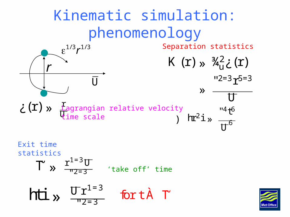
Kinematic simulation: phenomenology
U
r
2/3
1/3
rr
U
1/3 1/3 r
¿(r) » rU
~T » r 1=3U"2=3
hti » Ur 1=3
"2=3
Separation statistics
K (r) » ¾2u¿(r)
»"2=3r5=3
U
Exit time statistics
) hr2i »"4t6
U6
‘take off’ time
for t À ~T
Lagrangian relative velocity time scale

• Inertial range • 1200 modes• Unidirectional mean flow
• Adaptive time step based on local decorrelation time scale
Separation statistics
Exit time statistics
U(10;0;0) À ¾u = 1
L=́ = 106 ¡ 108

Mean exit time Mean square exit time
Mean inverse exit time
KSstatistics

KS pdf
½= 1:075

KS pdf
½= 2

Direct numerical simulation
• Homogeneous isotropic turbulence• cubic lattice• Taylor-scale Reynolds number • Two million Lagrangian particles• Sampling rate • • Data available from Cineca supercomputing
centre, Bologna, Italy
07.0
31024
280R
¿́ = 3:3¢10¡ 2, TL = 1:2, ´ = 5¢10¡ 3, L = 3:14, " = 0:81, C0 = 5:2

Mean exit time Mean square exit time
Mean inverse exit time
DNS statistics

DNS pdf
½= 1:075

Survival probability
• Probability that a pair will be in sphere of radius R after time t

DNS pdf
½= 2

DNS exit time pdfs
• No power law scaling for • Mean exit time lies within power law scaling
range for – relative velocity of average pair decreases faster than
decorrelation time scale – majority of pairs separate diffusively
• Exponential decay of tail agrees with diffusive behaviour for – only slow separators are diffusive– observed with low probability
• Self-similarity of tail decreases with increasing • For tail of pdf affected by and L• Tail of pdf for is ‘stretched’ version of
tail for
2
075.1
2
075.12
075.1

Richardson’s constantScaling of exit time moments according to K41
Since Cn(½) = Fn(½)k¡ n0 and g= 1144=81k3
0 weget
htn i = Cn(½)r2n=3="n=3
Require model to relate Cn(½) to g
Richardsons di®usion equation with K (r) = k0"1=3r4=3
g =114481
r2
"
µFn(½)htn i
¶3=n

Richardson’s constantfrom positive moments
½= 1:075
½= 2

Richardson’s constant II
• Finite duration of simulation– slowest separators do not have time to reach large r
• Statistical noise
• Intermittency
• Velocity memory– little impact on higher positive moments– likely to affect negative moments
² g calculated from mean exit timeappears to be independent of ½
² ´ and L e®ects
{ extent of plateau increases with decreasing ½
{ greater e®ect for ½À 1 than for ½¡ 1¿ 1
{ h1=t3i independent of mean dissipation rate{ small but a®ects ½¡ 1¿ 1 more than ½À 1
{ statistics for decreasing ½and r increasingly noisy

Richardson’s constant from negative moments
Cn(½) = An(½)g¡ n=3
Dimensional arguments ) Cn(½) / k¡ n0
g=r2
"
µht¡ n iA¡ n
¶3=n
A¡ n calculated from stochastic di®erential equationcorresponding to di®usion equation

Richardson’s constantfrom negative moments
½= 1:075
½= 2

Richardson’s constant from negative moments II
• Exit times for DNS larger (slower) than for diffusive process
• Inverse exit times for DNS smaller than for diffusive process
g will decreasewith decreasing ½
) h1=ti factor of ½¡ 1 too small
g» (½¡ 1)3 for ½¡ 1¿ 1
² Since T̂B is correct timescale for DN S for ½¡ 1¿ 1
² g calculated from h1=ti scales like

Richardsons constant calculated from h1=ti

Lagrangian stochastic model
• Quasi-one-dimensional
• Magnitude of separation calculated from longitudinal relative velocity
• Treat r and vr jointly as continuous Markov process
• Assume infinite inertial subrange
• C0 enters model explicitly
– can study effects of velocity memory

Lagrangian stochastic model II
• Pdf of Eulerian velocity difference– weighted sum of three Gaussians– constructed such that first three
moments are consistent with K41
a0 = C0dlnf E
d»¡
73f E
Z »
¡ 1»0f E (»0) d»0
d»="1=3
r2=3a0(»)dt +
"1=6
r1=3
p2C0dW(t)
dr = ("r)1=3»dt
Drift term Diffusion term
»= (vr =r)1=3

Richardson’s constant from positive moments of Q1D model

Richardson’s constant from negative moments of Q1D model

² Error larger for smaller ½² Error decreases monotonically with n for ½= 2
² For ½= 1:075 error decreases monotonically only for n > 1
² Mean invariant to ½
² Error decreases with increasing C0
Richardson’s constantcalculated from positivemoments
² Error largest for second order moment for ½= 1:075

Richardson’s constant from positive moments II
g =114481
r2
"
µFn(½)htn i
¶3=n
Richardson’s constant calculated from
For di®usiveprocess Fn(½) and htn i scale like½¡ 1
) g» (½¡ 1)3(1¡ n)=n
For ½¡ 1¿ 1
For ballistic process htn i scales like (½¡ 1)n
Independent of ½for n = 1

g calculated fromht2i for C0 = 1

Conclusions
• Physics of separation process intimately related to spacing of thresholds
• Kinematic simulation reaches its diffusive limit earlier than real turbulence
• In real turbulence velocity memory is important
• Spacing of thresholds and order of moment important for calculating Richardson’s constant
di®usive limit reached only for large½