Existence of Invariant Norms in p-adic Representations of ...eassaf/AssafEran_PhD thesis.pdf ·...

Existence of Invariant Norms in p-adicRepresentations of Reductive Groups

Thesis submitted for the degree of Doctor of Philosophy

by

Eran Assaf

Submitted to the Senate of the Hebrew University of Jerusalem

November 2016

This work was carried out under the supervision ofProf. Ehud de Shalit

Acknowledgements

First and foremost, I would like to thank my advisor, Prof. Ehud de Shalit, for hisguidance. Udi’s intuition and ideas significantly aided my research, and helped methink differently about mathematics. Udi has also introduced me to the academic worldin general, and important events in our field of research, in particular. His naturalamity and optimistic views, combined with his willingness to improve processes in theuniversity and in our society in general, has impressed and inspired me greatly.

Next, I would like to thank my thesis committee - Prof. David Kazhdan and Prof.Michael Schein - for their time and insights. In addition, I would like to thank David forintroducing me to algebraic groups, and for his mathematical and meta-mathematicalideas and advice throughout my studies. Even though this work is very technical,David’s views about simplicity in mathematics have helped me to see things moreclearly.

I would also like to thank my fellow graduate students for their friendship, and manyhelpful talks and ideas. Special thanks are due to Uri Brezner and his profound under-standing of algebraic geometry, to Adina Cohen for many fruitful discussions, to AmitOphir and Oren Becker for our special seminar, to Cy Maor for tea and council, and tomy officemates Yatir Halevi and Ohad Drucker.

Finally, I would like to thank my wife and family for their support all throughout mystudies, which has enabled this research.

2

Abstract

This thesis lies in the framework of the p-adic Langlands programme, whose goal

is to deepen our understanding about fundamental problems in number theory, such

as the solution of Diophantine equations, the study of elliptic curves, and the study

of Shimura varieties. The Langlands programme aims at creating a correspondence

between certain representations of Galois groups and certain representations of the

Adelic points of suitable reductive groups. An important and interesting particular

case is class field theory, in which such a correspondence has been established,

between characters of the Galois group and Dirichlet characters of the Ideles.

As a part of the Langlands programme, Robert Langlands has introduced the

Local Langlands Conjectures, which describe a correspondence between complex

representations of a reductive algebraic group G over a local field F and homomor-

phisms of the Galois group of F into the L-group of G. These conjectures have been

proven for G = GL(n) and for several other cases. This correspondence is preserved

in l-adic representations, where l is not the characteristic of the residue field of F.

However, when l = p is the characteristic of the residue field of F, this correspondence

no longer holds.

The purpose of the p-adic Langlands programme is to create a similar correspon-

dence between some of the p-adic representations of the reductive group, and some

of the p-adic representations of the Galois group. Such a correspondence has been

shown for G = GL(2) when the field is Qp. In this case, the representations of Gwhich took part in the correspondence were Banach spaces with a G-invariant norm.

In the cases where the representation of the Galois group is geometric, these spaces

have algebraic vectors (that the G-action on them is locally polynomial) which form

a locally algebraic representation of G with a G-invariant norm, dense in the original

Banach space.

The relation between these spaces and the representations of the Galois group

raised the possibility of generalizing the correspondence to other fields or other

groups by looking at the locally algebraic representations of the reductive group G,

finding G-invariant norms and completing with respect to these norms to obtain

Banach Spaces which are the candidates to correspond to the appropriate represen-

tations of the Galois group.

Therefore, Breuil and Schneider conjectured a criterion for the existence of an in-

variant norm in a p-adic representation of the group G = GL(n), and even generalized

it to an arbitrary split reductive group.

In this work, we prove several special cases of this conjecture. The problems

3

considered here can be classified into two interconnected topics – the existence of

invariant norms in locally algebraic representations of GL(2) over a local field, and

the existence of invariant norms in locally algebraic representations of U(3) over a

local field.

The methods employed in this thesis can also be classified into two essential

types - one method is reduction of the problem to pure p-adic analysis, which we

could only perform for G = GL(2), while the other methods use the homology of

the Bruhat-Tits tree of the reductive group G, and could be generalized to arbitrary

unramified groups by employing similar methods on the Bruhat-Tits building, with

increasing technical difficulty.

In Chapter 2, we prove the existence of an invariant norm in locally algebraic

representations of GL(2) over a local field, when the Breuil-Schneider criterion holds,

for unramified representations of small weight, and for smooth tamely ramified

representations. Even though both results have been known before, each result was

proved in a different method, and this is the first method proving both.


representations of GL(2) over a local field, when the Breuil-Schneider criterion holds,

for some unramified representations of higher weights. Apart from the restriction

on the weight, we have here a technical restriction on the representation, which we

could not remove, but we estimate that it is purely technical.


representations of U(3) over a local field, when the Breuil-Schneider criterion holds,

for unramified representations of small weight, and for smooth tamely ramified

representations. Each result is achieved using a different method.

None of the chapters have been published yet.

4

Letter of Contribution

This thesis contains three papers.

Two of the papers, included as chapters 3 and 4, are authored by Eran Assaf, and arethe result of Eran Assaf’s research during his PhD studies under the supervision of theadvisor, Prof. Ehud de Shalit. Both papers are still unpublished.

The paper ”Kirillov models and the Breuil-Schneider conjecture for GL2(F)”, included aschapter 2 in this thesis is authored by Eran Assaf, David Kazhdan and Ehud de Shalit,and remains unpublished. The following paragraphs clarify the different contributionsof each author, as required by the Hebrew University in order to include the paper as apart of Eran Assaf’s Ph.D. thesis.

David Kazhdan initiated the research project that eventually led to this paper. Hesuggested the idea of using Kirillov models in order to reduce the problem to p-adicanalysis, but most mathematical work (including the precise definitions, claims andproofs) has been done by Ehud de Shalit and Eran Assaf, who are the two equal maincontributors for this paper. This paper is a direct continuation and generalization of aprevious paper authored by David Kazhdan and Ehud de Shalit, which only deals withthe smooth case.

Roughly speaking, Eran Assaf’s contribution to the paper lies mainly in the exceptionalcase and the simplification of the tamely ramified case, and Ehud de Shalit’s contributionto the paper lies mainly in introducing the lattices, establishing the recursion relations,and proving the unramified case. In particular, Section 2, which describes the prelimi-naries on Fourier analysis, lattices and the Kirillov model, and Section 3, which describesthe proof of the unramified case are due to Ehud de Shalit. Due to Eran Assaf are Section4, which describes the proof in the tamely ramified case, and Section 5, which describesthe proof in the exceptional case.

Prof. Ehud de Shalit

Eran Assaf

5

Contents

1 Introduction 7

2 Kirillov models and the Breuil-Schneider conjecture for GL2(F) 27

3 Existence of Invariant Norms in p-adic Representations of GL2(F)of Large Weights 44

4 Existence of Invariant Norms in p-adic Representations of U3(F) 87

6

1 Introduction

The p-adic local Langlands programme

Let p be a prime number, and let n be a positive integer. Let F be a finite extension ofQp,and let WF be the Weil group of F. Let l be a prime number, such that l , p.

Local class field theory gives an isomorphism between the abelianization of the Weilgroup, Wab

F and the multiplicative group F×. Equivalently, we have a natural bijectionbetween complex (resp. l-adic) continuous characters of WF and complex (resp. l-adic)smooth characters of F×.

This theory has a non-abelian generalization, the local Langlands correspondence. The(classical) local Langlands correspondence for GLn over p-adic fields, proved by Harrisand Taylor [16], by Henniart [17], and later by Scholze [23] asserts the existence of acanonical bijection between the set of isomorphism classes of irreducible continuouscomplex (resp. continuous l-adic, see Vigneras [27]) representations of WF of dimen-sion n and the set of isomorphism classes of complex (resp. l-adic) smooth irreduciblesupercuspidal representations of GLn(F).

This correspondence is moreover compatible with reduction modulo l ([25]) and withcohomology ([16]).

The original aim of the local p-adic Langlands programme is to look for a possible p-adicanalogue of the classical and l-adic correspondence, stated in the previous subsection.

Note that when considering continuous p-adic representations, Grothendieck’s l-adicmonodromy theorem no longer holds, and we might have wild ramification that cannotbe solved by passage to a finite extension of F. This shows that we have a richer categoryof representations of WF in the p-adic case, while the category of smooth representationsof GLn(F) does not see the field of coefficients, hence remains the same. This suggests thatone needs to enlarge the category considered on the reductive side, and that one indeedneeds a p-adic correspondence, which essentially differs from the l-adic correspondence.

The local p-adic correspondence for GL2(Qp) was fully developed, essentially by Berger,Breuil and Colmez in [2], [8] and completed by Colmez, Dospinescu and Paskunas in[9], using the theory of (ϕ,Γ)-modules.

The p-adic local Langlands correspondence associates to certain 2-dimensional contin-

7

uous representations of Gal(Qp/Qp), certain Banach spaces equipped with a unitarycontinuous action of GL2(Qp). It has three important compatibility properties:

• compatibility with reduction modulo p [1]

• compatibility with classical local Langlands correspondence [8, 12]

• local-global compatibility with completed etale cohomology [12]

These properties already have remarkable global applications. For example, Kisinshows in [20] that the compatibility with the classic local Langlands correspondence,under some weak technical assumptions, implies the Breuil-Mezard conjecture on mod-ular multiplicities [5]. Combined with the proof of Serre’s modularity conjecture byKhare-Winterberger-Kisin, Emerton’s local-global compatibility then allows one to provemany cases of the Fontaine-Mazur conjecture, which characterizes the representationsof Gal(Q/Q) arising from classical modular forms.

If F is a finite extension of Qp, it is natural to ask how to associate p-adic representationsof GL2(F) to 2-dimensional p-adic representations of Gal(F/F). This problem turns outto be far more delicate when F , Qp and even the theory modulo p for GL2(F) is verymuch involved. Furthermore, as Colmez’s technique in [8] specifically associates to a(ϕ,Γ)-module a 2-dimensional representation of the Galois group, it is not clear yet howto approach the case of GLn(F) for n > 2, even when F = Qp, or more generally, theF-points of an arbitrary reductive group G.

In order to obtain a first approximation to what we might expect in such cases, wewill first introduce some notions regarding Banach space representations of reductivegroups, and then recall some of the constructions arising when n = 2 and F = Qp.

Representations of Reductive Groups

Let C be a field of characteristic 0, used as the field of coefficients.

Let G be a connected reductive group defined over F, a finite extension of Qp, and setG = G(F).

Definition 1. Smooth Representation

A representation π : G→ GL(V) on a C-vector space V is called smooth if the stabilizer of eachvector v ∈ V is open in G.

8

Definition 2. Smooth Admissible Representation

A smooth representation π : G→ GL(V) on a C-vector space V is called admissible if for everyopen subgroup H ⊆ G the space VH of H-invariants in V is finite-dimensional.

The following theorem is highly important in the development of the theory of smoothrepresentations, and was proved by Jacquet in [19]

Theorem 3. Let (π,V) be an irreducible smooth representation of G. Then (π,V) is admissible.

We now focus our attention on the case where C is p-adic.

Assume from now on that C is a finite extension ofQp, OC its ring of integers. Let $ ∈ OC

be a uniformizer, and κC = OC/$OC the residue field, of cardinality q. Let | · | denote theabsolute value on C, normalized so that |$| = q−1.

As we mentioned before, in this case, it is reasonable to introduce larger classes of rep-resentations, since enriching the category of representations of the reductive groups isnecessary for extending the local Langlands correspondence to p-adic Galois representa-tions. First, as in the l-adic case (see Vigneras, [27]), we introduce the notion of a unitaryBanach space representation.

Definition 4. Unitary Banach Space Representation

Let (V, ‖ · ‖) be a Banach C-vector space. A Unitary C-Banach space representation of G (onV) is a G-action by continuous linear automorphisms such that the map G × V → V giving theaction is continuous, and given by isometries, i.e. for all g ∈ G and all v ∈ V

‖gv‖ = ‖v‖.

In order to motivate what follows, we would like to mention two pathologies of Banachspace representations:

• There exist non-isomorphic topologically irreducible Banach space representationsV and W of G for which nevertheless there is a nonzero G-equivariant continuouslinear map V →W (similarly to the case of real Lie groups).

• Even such a simple commutative group such as G = Zp has infinite dimensionaltopologically irreducible Banach space representations (see [11]).

9

It is clear that in order to avoid such pathologies we have to impose an additionalfiniteness condition on our Banach space representations. This condition will be calledadmissiblity, and in a series of papers, Schneider and Teitelbaum found out what seemsto be the right notion (see [21]).

Definition 5. Admissibility

Let G be a finite dimensional p-adic Lie group. A C-Banach space representation V of G iscalled admissible if there is a G-invariant bounded open lattice L ⊆ V such that for any opennormal subgroup H ⊆ G the κC-vector space (L/$L)H of H-invariant elements in L/$L is finitedimensional.

We point out that this condition implies that V is admissible if and only if there isa G-invariant bounded open lattice L ⊆ V such that L/$L is an admissible smoothrepresentation of G over the residue field κC.

The following proposition, which is proved by Schneider and Teitelbaum in [21, Lemma3.4] and the discussion following it, shows that it is enough to check the condition for asingle open normal subgroup H ⊆ G which is pro-p. Moreover, Schneider and Teitelbaumshow that if one considers the invariants by such an open normal pro-p subgroup, onecan take any open G-invariant lattice.

Proposition 6. Let V be a C-Banach space representation of G. Let H ⊆ G be an open normalpro-p subgroup. Assume that there is a G-invariant bounded open lattice L ⊆ V such that theκC-vector space (L/$L)H of H-invariant elements in L/$L is finite dimensional. Then V isadmissible.

Conversely, if V is admissible, then for any G-invariant bounded open lattice L ⊆ V, the κC-vectorspace (L/$L)H of H-invariant elements in L/$L is finite dimensional.

The p-adic local Langlands correspondence for GL2(Qp) (see [2], [8] and [9]) gives a bijec-tion between isomorphism classes of 2-dimensional absolutely irreducible continuousrepresentations of Gal(Qp/Qp) over C and isomorphism classes of absolutely irreducible,non-ordinary, admissible unitary Banach representations of GL2(Qp) over C.

Restricting the bijection to the potentially semi-stable Galois representations, with dis-tinct Hodge-Tate weights, one obtains an important subcategory on the reductive side,consisting of completions of irreducible locally algebraic representations.

For this reason, we proceed to define locally algebraic representations. But first, let usdefine an algebraic representation.

10

LetG :=

(ResF/QpG

)C

be the reductive group over C obtained by base extension from the Weil restriction fromF to Qp of G. Write

G := G(C) = G(F ⊗Qp C).

The ring homomorphism F → F ⊗Qp C which sends a to a ⊗ 1 induces an embedding ofgroups G ↪→ G.

Definition 7. Let (τ,V) be a representation of G on a C-vector space. Then τ is algebraic ifthere is a rational representation τ of G on V such that τ is the pullback of τ via G ↪→ G.

We now turn to the definition of a locally algebraic representation.

Definition 8. Let (π,V) be a representation of G over C. We say that v ∈ V is locally algebraicif there exists a compact open subgroup Kv ⊆ G and a finite dimensional subspace U ⊆ Vcontaining the vector v such that Kv leaves U invariant and operates on U via restriction to Kv ofa finite dimensional algebraic representation of G. We denote by Valg

⊆ V the subspace of locallyalgebraic vectors. If V = Valg, we say that V is locally algebraic.

An important result, proved by Prasad in [22, Appendix], gives an explicit descriptionof the irreducible locally algebraic representations of G.

Theorem 9. Let π be an irreducible locally algebraic representation of G. Then there is anirreducible algebraic representation τ of G, and an irreducible smooth representation σ of G, suchthat π = τ ⊗ σ. Conversely, if τ and σ are as above, then π is an irreducible locally algebraicrepresentation of G.

This will allow us to restrict our attention mostly to representation of the form π = τ⊗σ.

The Breuil-Schneider Conjecture

We would like to formulate a p-adic correspondence for arbitrary n and F. In order tohave an idea as to how such a correspondence should be obtained, let us take anotherlook at the construction of the correspondence for GL2(Qp).

In general, for potentially semi-stable n-dimensional continuous representations of theabsolute Galois group Gal(F/F), it is possible to attach a smooth representation σ = σ(ρ) of

11

GLn(F), as in the classical case. However, ρ σ(ρ) is no longer reversible. Nevertheless,as the coefficient field is now an extension ofQp, if we assume that ρ has distinct Hodge-Tate weights, we may also construct an irreducible algebraic representation τ = τ(ρ) ofGLn(F) from the Hodge-Tate weights of ρ. We will specify the explicit construction whenformulating the conjecture subsequently.

Still, one cannot reconstruct ρ from σ(ρ) and τ(ρ). The problem is that the semi-stablerepresentations ρ are classified by their filtered (ϕ,N)-modules, and not only by their(ϕ,N)-modules and the Hodge-Tate weights. The Hodge filtration is lost when con-structing the representations τ(ρ) and σ(ρ). Note that as the coefficient field is p-adic,these two representations live in the same universe, and it makes sense to consider therepresentation π = σ ⊗ τ. These representations are no longer smooth, neither are theyalgebraic, but they are locally algebraic.

The p-adic local Langlands correspondence for GL2(Qp) takes any continuous represen-tation ρ : Gal(Qp/Qp)→ GL2(Qp) and attaches to it a unitary Banach space Π(ρ) with anadmissible unitary GL2(Qp)-action. This map ρ Π(ρ) is reversible, and compatiblewith classical local Langlands in the following sense: When ρ is potentially semistablewith distinct Hodge-Tate weights,

Π(ρ)alg = τ(ρ) ⊗Qpσ(ρ)

Furthermore, Π(ρ)alg = 0 otherwise (see [8, Theorem VI.6.13]).

When ρ is irreducible, Π(ρ) is known to be the completion of τ(ρ) ⊗Qpσ(ρ) relative to a

suitable GL2(Qp)-invariant norm ‖·‖which corresponds to the lost Hodge filtration.

As for a general field F, if ρ : Gal(F/F) → GLn(Qp) is potentially semi-stable , one candefine the representation π = BS(ρ) := τ(ρ) ⊗Qp

σ(ρ). This representation is a densesubrepresentation of a unitary GLn(F) Banach representation Π(ρ) if and only if it admitsa GLn(F)-invariant norm.

This suggests, at least as a first approximation, that the existence of such an invariantnorm will be equivalent to having a representation corresponding to a potentially semi-stable representation.

We now formulate the conjecture more precisely.

Let G = GLn(F), n ≥ 2. Let F′ be a finite Galois extension of F, and F′0 its maximalunramified subfield. Assume [F′0 : Qp] = |HomQp(F

′

0,C)| and let p f ′ be the cardinality

12

of the residue field of F′0 and ϕ′

0 the Frobenius on F′0 (raising to the p-th power eachcomponent of the Witt vectors).

Let ModF′/F be the category of discrete finite dimensional (ϕ,N,Gal(F′/F))-modules. LetWDF′/F be the category of finite dimensional Weil-Deligne representations over C whichare unramified when restricted to W(F/F′). Fontaine, in [14], constructs a functor WD :ModF′/F →WDF′/F which induces an equivalence of categories.

Now, if (ρ,N,V) is an object of WDF′/F such that ρ is semisimple, we have by the classicallocal Langlands correspondence, a smooth irreducible representation of G over Qp, σunit

corresponding to (ρ,N,V), normalized so that the central character of σunit is det(r,N,V)◦Art−1

F , with ArtF being Artin’s reciprocity map from local class field theory, sendinguniformizers to geometric Frobenii. Note that σunit depends on a choice of q1/2 in Qp.

Breuil and Schneider in [6] construct a modification, σ of σunit, which does not dependon the choice of q1/2, and is a smooth representation of G over C. If (ρ,N,V) is an objectof WDF′/F we denote by (ρ,N,V)ss its ρ-semisimplification.

Conjecture 10. The Breuil-Schneider Conjecture

Fix an object (ρ,N,V) of WDF′/F such that ρ is semisimple. For each ι : F ↪→ C, fix a list of nintegers i1,ι < i2,ι < . . . < in,ι. Let σ be the smooth representation of G over C described above. Leta j,ι = −in+1− j,ι − ( j − 1) and denote by τ the unique Qp-rational representation of G over C suchthat τ = ⊗ιτι with τι of highest weight (a1,ι, . . . , an,ι).

The following conditions are equivalent:

1. There is an invariant norm on τ ⊗C σ.

2. There is a (ϕ,N,Gal(F′/F))-module D such that

WD(D)ss = (ρ,N,V)

and an admissible filtration (FiliDF′,ι)i,ι preserved by Gal(F′/F) on DF′ := F′ ⊗F0 D suchthat ∀ι : F ↪→ C

FiliDF′,ι/Fili+1DF′,ι , 0 ⇐⇒ i ∈ {i1,ι, . . . , in,ι}.

This asserts that the existence of an invariant norm on τ⊗Cσ is equivalent to the existenceof a (weakly) admissible filtered (ϕ,N,Gal(F′/F))-module, the semisimplification of itsimage being (ρ,N,V), namely (ρ,N,V) is becoming semi-stable over F′.

13

By the equivalence of categories stated by Fontaine, and proved by Colmez-Fontaine,the conjecture predicts that the existence of an invariant norm on τ ⊗C σ is equivalent tothe existence of a potentially semi-stable representation V of GF of dimension n over C,such that its Hodge-Tate weights are the −i j,ι and such that the ρ-semisimplification ofits associated Weil-Deligne representation has σ as a Langlands parameter (modified asabove).

The “if” part is completely known for GLn(F) ([18]), and is due to Y. Hu. The “only if”part remains open, even for n = 2.

Next, we introduce the notion of an integral structure, whose existence in a representationis equivalent to the existence of a G-invariant norm.

Definition 11. Integral Structure

Let V be a representation of G on a C-vector space. An integral structure in V is an OC[G]-submodule which spans V over C and contains no C-line.

An integral structure is also referred to in the literature as a separated lattice.

Note that asking for a norm in a representation V over C, a finite extension of F, amountsto asking for an integral structure, that is a sub-OC[GLn(F)]-module generating V overC which contains no C-line: Given a norm || · ||, the unit ball is an integral structure.Conversely, given an integral structure Λ, its gauge ||x|| = q−vΛ(x)

C , where vΛ(x) = sup{v |x ∈ $vΛ} is a norm. Thus we are looking for integral structures in locally algebraicrepresentations of GLn(F).

The equivalence of norms gives rise to an equivalence relation on lattices, called com-mensurability. Explicitly, two integral structures in a representation are commensurableif each of them is contained in a scalar multiple of the other. Note that any two finitelygenerated integral structures are commensurable, hence of minimal nonzero commen-surability class.

Already in [6], the authors discuss a generalization to the case of an arbitrary splitreductive group G. In fact, they construct a Banach space for any pair (ξ, ζ) where ξ is adominant weight of the split torus T and ζ ∈ T′, the torus of the Langlands dual group.Given this pair, they construct a family of p-adic Galois representations with values in theLanglands dual group G′. Conjecture 10 is then equivalent to asserting that this Banachspace is nonzero for G = GLn(F). We note that this conjecture can be formulated purelyin terms of the reductive group G, ignoring the original Weil-Deligne representation. In

14

order to do so, we recall Emerton’s treatment of these ideas ([13]).

Emerton’s condition and arbitrary reductive groups

In [22], Prasad shows that any irreducible locally algebraic representation of a p-adicreductive group, G, is of the form σ ⊗ τ with σ smooth and τ algebraic. Moreover,V = σ ⊗ τ is irreducible if and only if both σ and τ are irreducible. If V admits a G-invariant norm, the central character must be unitary. Let P be a parabolic subgroup ofG, with unipotent radical N and Levi quotient M. Let N0 be some compact open subgroupof N. Let δ denote the modulus character of P (which is trivial on N, and so induces acharacter of M = P/N, which we also denote by δ; concretely, δ(m) = [mN0m−1 : N0]). LetJP(V) denote Emerton’s Jacquet module (with respect to P) of V, i.e. if V = σ ⊗ τ, then

JP(V) = τN⊗C (resG

Pσ)Nδ1/2

Let ZM be the center of M. Write Z+M := {z ∈ ZM | zN0z−1

⊂ N0}.

Lemma 12. (Emerton)

Let χ be a locally algebraic C-valued character of ZM. If the χ-eigenspace of JP(V) is nonzero, andV admits a G-invariant norm, then∣∣∣χ(z)δ−1(z)

∣∣∣ ≤ 1 ∀z ∈ Z+M

In [18], Hu shows that this is equivalent, in the case of GLn(F), to the requirement thatV arises from a potentially semi-stable Galois representation. Thus, it makes sense toreformulate the conjecture for arbitrary reductive groups.

Conjecture 13. Assume that for any locally algebraic character χ : ZM → C× with JP(V)χ , 0,∣∣∣χ(z)δ−1(z)∣∣∣ ≤ 1 ∀z ∈ Z+

M

and that the central character of V is unitary. Then V admits a G-invariant norm.

15

Progress on the Breuil-Schneider conjecture

• Note that the central character of BS(ρ) always attains values in O×C. Sorensen ([24])has proved for any connected reductive group G defined over Qp, that if τ is anirreducible algebraic representation of G(Qp), and σ is an essentially discrete seriesrepresentation of G(Qp), both defined over C, then τ ⊗C σ admits a G(Qp)-invariantnorm if and only if its central character is unitary.

• On 2013 there has been spectacular progress on the BS conjecture in the principalseries case, which is the most difficult, by joint work of Caraiani, Emerton, Gee,Geraghty, Paskunas and Shin ([7]). Using global methods, they construct a candi-date Π, which could depend on some global data in addition to ρ, for a p-adic localLanglands correspondence for GLn(F) and are able to say enough about it to provenew cases of the conjecture. Their conclusion is even somewhat stronger than theexistence of a norm on BS(ρ), in that it asserts admissibility.

Both works employ global methods, and as this is a question of local nature, we believethat there must be some local method to recover these results. There has also been someprogress employing local methods, which yields results also for finite extensions of Qp,namely:

• For GL2(F), Vigneras ([26]) constructed an integral structure in tamely ramifiedsmooth principal series representations, satisfying the assumption that they arisefrom p-adic potentially semistable Galois representations.

• For GL2(Qp), Breuil ([4]) used compact induction together with the action of thespherical Hecke algebra to produce a separated lattice in BS(ρ) where π = BS(ρ) isan unramified locally algebraic principal series representation, under some tech-nical p-smallness condition on the weight. This was later generalized to GL2(F) byde Ieso ([10]).

• For general split reductive groups, Große-Klonne ([15]) looked at the universalmodule for the spherical Hecke algebra, and was able to show some cases of theconjecture for unramified principal series, again under some p-smallness conditionon the Coxeter number (when F = Qp) plus other technical assumptions.

16

New cases of the Breuil-Schneider conjecture

Let p be a prime number. Let F be a finite extension of Qp. Fix a uniformizer $ of F, andlet q be the cardinality of its residue field κF = OF/$OF. Let vF : F× → Z be the valuationon F normalized so that vF($) = 1. Let C be a finite extension of F. Here and in whatfollows, we fix one embedding F ↪→ C and consider the special case of Conjecture 10where the algebraic representation τ is trivial for the other embeddings.

Let G be a reductive group over F and let G = G(F) be the group of its F-points.

In this work, we consider the principal series representations of the reductive groups G,and prove the existence of invariant norms in some of these representations. The caseof locally algebraic principal series representations seems to be the most difficult whenconsidering the existence of G-invariant norms, or equivalently an integral structure.

Quite generally, if G is an arbitrary reductive group, and π = τ ⊗ σ is an irreduciblelocally algebraic representation of G = G(F), the simpler σ is algebraically, the harder thequestion of existence of G-invariant norms inπbecomes. An obvious necessary conditionis for the central character of π to be unitary, i.e. attain values in O×C. Assume thereforethis is the case. If σ is supercuspidal (its matrix coefficients are compactly supportedmodulo the center), the existence of a G-invariant norm is obvious. As mentionedabove, using global methods and the trace formula, existence of a G-invariant norm canalso be proved when σ is essentially discrete series (its matrix coefficients are squareintegrable modulo the center) [24]. In these cases, no further restrictions are imposed onπ. At the other extreme stand principal series representations, where one should imposesevere restrictions on π, and the problem becomes very difficult. We therefore focus ourattention on these representations.

In this thesis we show the existence of a G-invariant norm by showing the existence of anintegral structure, hence the completion with respect to the resulting norm is nonzero.However, we do not show admissibility of the resulting completion. In some cases,we consider a finitely generated integral structure, hence the resulting completion isnecessarily the universal completion, which is known to be non-admissible, for example,when F , Qp (see [3]).

We consider two specific groups - the group GL2(F) is considered in chapters 2 and 3,while in chapter 4 we consider the unitary group U3(F).

17

Studying the Kirillov Model for GL2(F)

In chapter 2, we provide a proof of two results, which were until now proved in twodifferent methods, using a unified and new framework. We prove the Breuil-Schneiderconjecture for both smooth tamely ramified principal series representations and unram-ified locally algebraic principal series representations of small weight. This is achievedby looking at the Kirillov model of the representation, and transforming the question onintegral structures to a problem in p-adic analysis.

In order to state the result more precisely, let χ1, χ2 be smooth characters of F× attainingvalues in C×, let B be the Borel subgroup of upper triangular matrices in G = GL2(F) andlet

σ = IndGB (χ1, χ2)

be the smooth (not normalized!) principal series representation induced from the char-acter χ1 ⊗ χ2, viewed as a character on the torus of diagonal matrices, and inflated toB. Explicitly, we require f (bg) = (χ1 ⊗ χ2)(b) · f (g)∀b ∈ B, g ∈ G. Assume that χ1, χ2 arechosen such that σ is irreducible. Fix integers m and n ≥ 0, and let

τ = det(·)m⊗ Symn

where Symn denotes the n-th symmetric power of the standard representation of G. Weuse the space of univariate polynomials of degree at most n, C[u]≤n, as a model for therepresentation Symn.

The Breuil-Schneider conjecture for π = τ ⊗ σ asserts that π admits an integral structureif and only if the following two conditions are satisfied:

(i)∣∣∣χ1($)χ2($)$2m+n

∣∣∣ = 1

(ii) 1 ≤ |χ1($)$m| ≤

∣∣∣q−1$−n∣∣∣

It is known that these two conditions are necessary. In Chapter 2, we prove the followingtheorem.

Theorem 14. Assume that (i) and (ii) are satisfied. Assume, in addition, that either

(1) χ1 and χ2 are unramified and n < q, or

(2) χ1 and χ2 are tamely ramified and n = 0.

18

Then π admits an integral structure.

Each of the cases (1) and (2) was already known ([26], [4], [10]), but treated separately.Here, using the study of the Kirillov model of the representation π, one can transformthe problem to a problem in p-adic functional analysis, and use it to prove both cases.The restrictions on ramification level and algebraic weight are also needed in the afore-mentioned works. In fact, this is true even though Breuil, de Ieso and Vigneras all usethe method of compact induction, working on the Bruhat-Tits tree of G = GL2(F), whileour approach takes place in a certain dual space.

The Kirillov model K of π is the space of functions on F×

K = C∞c (F, τ)χ1 + C∞c (F, τ)ωχ2

where ω is the norm character, namely the unramified character satisfying ω($) = q−1,and C∞c (F, τ) is the space of smooth compactly supported functions on F with values inτ. For the action of G on this model, see Chapter 2, Section 1.3.

Fourier analysis implies that an arbitrary function φ ∈ K may be expanded annulus-by-annulus as

φ =

∞∑l=l0

∑β∈F/OF

Cl(β)φl,β

for some l0 ∈ Z, some predetermined functions φl,β ∈ C∞c (F,C), which are supported on$lO×F and the coefficients Cl(β) ∈ τ satisfy certain explicit recursion relations.

The theorem is based on the following observation. Let the assumptions be as in thetheorem. If V0 is an OC[G]-module spanned by a nonzero vector in the Kirillov model K,one can find a family of OC-lattices (M0(β))β∈F/OF in τ, such that if φ ∈ V0 vanishes outsideof OF, it has an expansion as above with C0(β) ∈M0(β) for all β.

We note that while this claim is sufficient to prove the theorem, it is not clear that theyare equivalent.

The first step in the proof of this theorem is standard, showing commensurability be-tween V0 and a certain OC[B]-module of finite type Λ, which is spanned by an explicitset of nice functions E. If one considers φ ∈ Λ and expresses it as a linear combination ofthe functions in E, and expand it annulus-by-annulus, the Cl(β) satisfy certain recursiverelations. If one further assumes that φ vanishes away from OF, we must have somecancellation. By increasing induction, one shows that for l ≤ 0, the Cl(β) belong to a

19

certain OC-lattice Ml(β) in τ, which depends on l and β, but not on φ.

The main phenomenon which assists us in establishing the theorem is that there are twodistinct families of lattices, which coincide when n < q. In fact, for any β ∈ F/OF and anyinteger l, one may define the disc

Dl(β) ={α ∈ F |

∣∣∣α − $−lβ∣∣∣ ≤ ∣∣∣$−l

∣∣∣}and consider

Nl(β) ={P ∈ C[u]≤n

| |P(α)| ≤ |$|−nl∀α ∈ Dl(β)

}This family of lattices has the nice property that for any γ ∈ F/OF we have⋂

{β∈F/OF|πβ=γ}

Nl(β) = $nNl+1(γ) (1)

Similarly, one may define

Ml(β) = SpanOC

{($−l

)n−i (u − $−lβ

)i| 0 ≤ i ≤ n

}This family of lattices has the nice property that

Ml(β) ⊆Ml+1($β). (2)

When n < q, it turns out that Ml(β) = Nl(β). In this case, both properties combined withthe recursive relations on the coefficients, suffice to establish the proof.

However, when n ≥ q, this is no longer the case. In fact, if one begins with a familyof lattices Ml(β), we may modify it either to satisfy property (1) or property (2), call theresulting families M]

l (β) and M[l (β) respectively.

It turns out that if n ≥ q the process of performing the [ and ] operations alternatelyresults in modules which contain a C-line. This means that the approach taken here ofusing these properties combined with the recursive relations, essentially fails for n ≥ q.

The other drawback of this approach is that the Kirillov model has such an explicitdescription as a space of functions only for G = GL2(F). For other reductive groups,working with the Kirillov model is much more difficult, and no longer reduces theproblem purely to functional analysis. Furthermore, in the case of G = GL2(F), the

20

Kirillov model can be identified with a Fourier transform of the standard model (up tomultiplication by a character). For other reductive groups, this is no longer the case, andwhen the unipotent radical of B is no longer abelian, a possible approach is to replacethe Kirillov model with the non-abelian Fourier transform of the standard model, whichagain is much more complicated.

Large Algebraic Weights for GL2(F)

Although many results were obtained for representations of GL2(F), it has been verydifficult to prove the existence of GL2(F)-invariant norms in locally algebraic representa-tions of large weights, and all results known so far have severe restriction on the weights.In Chapter 3, we provide a proof of several results, establishing the existence of GL2(F)-invariant norms in many unramified locally algebraic representations of large weights.We employ methods developed by Breuil in [4] and by de Ieso in [10].

Keeping notations, we let τ = det(·)m⊗ Symn, and write n = d · q + r with 0 ≤ r < q.

We also set a = (χ−11 ($) + q · χ−1

2 ($)) · $−m∈ C. We further denote by e the ramification

degree of F over Qp. In this case, the Breuil-Schneider conditions are equivalent simplyto a ∈ OC. Then the main theorem we prove in Chapter 3 is

Theorem 15. Assume that one of the following conditions is satisfied:

(i) n ≤ 12q2 with r < q − d and vF(a) ∈ [0, 1].

(ii) n ≤ 12q2 with 2vF(a) − 1 ≤ r ≤ q − d and vF(a) ∈ [1, e].

(iii) n ≤ min(p · q − 1, 1

2q2), with d − 1 ≤ r and vF(a) ≥ d.

Then π admits an integral structure.

The proof of this theorem relies on the ideas of Breuil in [4], and it is highly technical andinvolved. The main idea is looking at ρ as a quotient of the universal spherical modulefor compact induction. This universal module has a natural integral structure, whoseimage under the quotient map is an excellent candidate to be an integral structure in ρ.The quotient is formed using the Hecke algebra, and the analysis is performed on theBruhat-Tits tree of G = GL2(F).

In fact, if τ0 is the OC-points of the algebraic representation τ, it can be viewed naturallyas a lattice in τ, which gives rise to the lattice indG

KZ(τ0) in indGKZ(τ), where K = GL2(OF) is

21

the standard maximal compact subgroup, Z = Z(G) is the center of G, and indGKZ is the

functor of compact induction.

Now, the representation indGKZ(τ) can be viewed as functions on the vertices of the Bruhat-

Tits tree, taking values in τ (up to a choice of a representative at each vertex). Denoteby BN ⊆ indG

KZ(τ) the subset of functions supported on the ball of radius N aroundthe standard chamber. Denote by T a Hecke operator generating the spherical Heckealgebra, normalized so that it is integral and $−1T is not.

Then, following Breuil, showing that indGKZ(τ0) is an integral structure reduces to the

following statement.

Theorem 16. Let the assumptions be as in the previous theorem. For all large enough N ∈ Z>0

there exists a constant ε ∈ Z≥0 depending only on N,n, a such that for all k ∈ Z≥0, and allf ∈ indG

KZ(τ) we have

(T − a)( f ) ∈ BN + $kindGKZτ0 ⇒ f ∈ BN−1 + $k−εindG

KZτ0.

Writing f =∑M

m=0 fm with fm supported on the sphere of radius N + m, one can show theabove by decreasing induction on m, using the explicit formula defining T.

The theorem and its proof are far from satisfying. There are many artificial restrictionsarising from this method of proof, since we rely on certain ”miracles” such as divisibilityof binomial coefficients and invertibility of certain matrices. Moreover, the proof depends(as in Breuil’s original proof for n < 2p) on a certain choice of representatives for κF inOF, namely the Teichmuller representatives. Except from being unnatural, it means thatgeneralization of this method to other reductive groups, where there is not always suchnice choice of representatives, is far from immediate. Indeed, the unipotent radical Nof the parabolic subgroup B is not as simple, and not always abelian. For example,if G = GL3(F), then N is the Heisenberg group. Therefore, we might not always haveTeichmuller representatives.

Moreover, it seems that there should be a more enlightening way of establishing thisresult, since one may reduce the statement of the theorem to a statement about I(1)-invariants of the reduction mod $k, where I(1) is the pro-p Iwahori subgroup corre-sponding to B, namely I(1) = red−1(N(κF)) with red the reduction mod $. This followsfrom the fact that we could restate it as the injectivity of a certain map between profi-nite I(1)-modules, which is equivalent to injectivity on the I(1)-invariants. However,

22

trying to establish the injectivity on the I(1)-invariants did not seem to be any easier, andconsequently is left out of the current work.

We hope that further study of the role of the I(1)-invariants in the reductions mod $k forG = GL2(F) and, more generally, the role of I(1)-cohomology for groups of higher rank,will lead to a more complete statement of the theorem in the future.

Invariant Norms for U3(F)

As many attempts were made in order to find criteria for the existence of integralstructures in representations of GL2(F), where F is a finite extension of Qp, towardsthe proof of the Breuil-Schneider conjecture, which concerns the case of GLn(F), andsomewhat more generally, the case of split reductive groups, very little is known aboutthe correspondence for non-split reductive groups, in particular for the unitary group.In chapter 4, we prove the existence of invariant norms in both smooth tamely ramifiedprincipal series representations of U3(F) and in unramified locally algebraic principalseries representations of U3(F) of small weight. We do so by employing the methodsdeveloped by Vigneras in [26] and by Große-Klonne in [15].

Let us state our result more precisely. Let E be a quadratic extension of F, and assumethat C contains also the normal closure of E. We also set for the rest of the introduction$ = $E a uniformizer of E (and not of F!!) and q = qE to be the cardinality of the residuefield of E. Let V be a 3-dimensional vector space over E, and let x 7→ x be the nontrivialinvolution in Gal(E/F). Denote by θ the Hermitian form on V represented by the matrix

0 0 10 1 01 0 0

with respect to the standard basis on V. Explicitly

(u, v) =tvθu.

LetG = U3(F) = U3(θ) =

{g ∈ GL3(E) | tgθg = θ

}Let B be its Borel subgroup of upper triangular matrices, and let M be the maximal

23

(nonsplit) torus of diagonal matrices contained in it. Letχ : E× → C× andχ1 : U1(F)→ C×

be smooth characters, where U1(F) ={x ∈ E | x · x = 1

}are the norm 1 elements. Then

one can consider χ ⊗ χ1 as a character of M, and inflate it to a character of B. We let

σ = IndGB (χ ⊗ χ1)

be the smooth principal series representation. Fix some a, b ∈ Z≥0 and some d ∈ Z. Let τbe the irreducible algebraic representation of U3 of highest weight

diag(z1, z2, z−11 ) 7→ za

1zb1 · det(g)d

with respect to B.

In chapter 4 we prove

Theorem 17. Assume that either

(i) χ, χ1 are unramified, and that a, b < p, or

(ii) χ, χ1 are tamely ramified, and that a = b = 0.

Then π admits an integral structure if and only if

|$|−a−b≤ |χ($)| ≤

∣∣∣q−2$−a−b∣∣∣

We note that this result holds both when E/F is unramified, and when E/F is ramified.Here, in contrast with chapter 2, the results are proved by two different methods. Case(i) is proved by the method of Breuil, as in [4], while case (ii) is proved by the methodVigneras uses in [26].

Although U3(F) is rank one, so the analysis on the Bruhat-Tits tree remains quite similarto GL2(F), its Borel subgroup already has a nonabelian unipotent radical, which com-plicates the computations. The existence of two conjugacy classes of maximal compactsubgroups, and the treatment of both ramified and unramified extensions E/F, whichyield different reductions, turned this generalization to be quite more involved than itappears to be.

We comment that although some of the methods employed in this work could be gener-alized to groups of higher rank, we wanted to focus on small rank, as there is still muchyet to understand already there.

24

References

[1] Laurent Berger. Representations modulaires de GL2(Qp) et representations galoisiennes de dimension2. Asterisque, 330:263–279, 2010.

[2] Laurent Berger and Christophe Breuil. Sur quelques representations potentiellement cristallines deGL2(Qp). Asterisque, 330:155–211, 2010.

[3] Christophe Breuil. Sur quelques representations modulaires et p-adiques de GL2(Qp): I. CompositioMathematica, 138(2):165–188, 2003.

[4] Christophe Breuil. Sur quelques representations modulaires et p-adiques de GL2(Qp): II. JOURNAL-INSTITUTE OF MATHEMATICS OF JUSSIEU, 2(1):23–58, 2003.

[5] Christophe Breuil and Ariane Mezard. Multiplicites modulaires et representations de GL2(Zp) et deGal(Qp/Qp) en ` = p. appendice par guy henniart. sur l’unicite des types pour gl2. Duke Math. J.,115(2):205–310, 11 2002.

[6] Christophe Breuil and Peter Schneider. First steps towards p-adic langlands functoriality. Journal furdie reine und angewandte Mathematik (Crelles Journal), 2007(610):149–180, 2007.

[7] Ana Caraiani, Matthew Emerton, Toby Gee, David Geraghty, Vytautas Paskunas, and Sug Woo Shin.Patching and the p-adic local langlands correspondence. arXiv preprint arXiv:1310.0831, 2013.

[8] Pierre Colmez. Representations de GL2 (Qp) et (φ, γ)-modules. Asterisque, 330(281):509, 2010.

[9] Pierre Colmez, Gabriel Dospinescu, and Vytautas Paskunas. The p-adic local langlands correspon-dence for GL2(Qp). arXiv preprint arXiv:1310.2235, 2013.

[10] Marco De Ieso. Existence de normes invariantes pour GL2. Journal of Number Theory, 133(8):2729–2755,2013.

[11] Bertin Diarra. Sur quelques repre´ sentations p-adiques de zp. In Indagationes Mathematicae (Proceed-ings), volume 82, pages 481–493. Elsevier, 1979.

[12] Matthew Emerton. Local-global compatibility in the p-adic langlands programme for GL2/Q. preprint,2010.

[13] Matthew Emerton et al. p-adic L-functions and unitary completions of representations of p-adicreductive groups. Duke Mathematical Journal, 130(2):353–392, 2005.

[14] Jean-Marc Fontaine. Representations l-adiques potentiellement semistables. Asterisque, (223):321–348, 1994.

[15] Elmar Große-Klonne. On the universal module of p-adic spherical hecke algebras. American Journalof Mathematics, 136(3):599–652, 2014.

[16] Michael Harris and Richard Taylor. The Geometry and Cohomology of Some Simple Shimura Varieties.(AM-151), volume 151. Princeton university press, 2001.

[17] Guy Henniart. Une preuve simple des conjectures de langlands pour GL (n) sur un corps p-adique.Inventiones mathematicae, 139(2):439–455, 2000.

25

[18] Yongquan Hu. Normes invariantes et existence de filtrations admissibles. Journal fur die reine undangewandte Mathematik (Crelles Journal), 2009(634):107–141, 2009.

[19] Herve Jacquet. Sur les representations des groupes reductifs p-adiques. CR Acad. Sci. Paris Ser. AB,280:A1271–A1272, 1975.

[20] Mark Kisin. The fontaine-mazur conjecture for GL2. Journal of the American Mathematical Society,22(3):641–690, 2009.

[21] Peter Schneider and Jeremy Teitelbaum. Banach space representations and iwasawa theory. Israeljournal of mathematics, 127(1):359–380, 2002.

[22] Peter Schneider, Jeremy Teitelbaum, and Dipendra Prasad. U(g)-finite locally analytic representa-tions. Representation Theory of the American Mathematical Society, 5(5):111–128, 2001.

[23] Peter Scholze. The local langlands correspondence for GL n over p-adic fields. Inventiones mathemat-icae, 192(3):663–715, 2013.

[24] Claus M Sorensen. A proof of the breuil-schneider conjecture in the indecomposable case. Annals ofMathematics, 177:1–16, 2013.

[25] Marie-France Vigneras. Correspondance de langlands semi-simple pour gl (n, f) modulo l, p.Inventiones mathematicae, 144(1):177–223, 2001.

[26] Marie-France Vigneras. A criterion for integral structures and coefficient systems on the tree of PGL(2, F). Pure and Applied Mathematics Quarterly, 4(4), 2008.

[27] Marie-France Vigneras et al. Banach l-adic representations of p-adic groups. Asterisque Journal, 327(1),2010.

26

2 Kirillov models and theBreuil-Schneider conjecture for GL2(F)

Eran Assaf, David Kazhdan and Ehud de ShalitUnpublished

27

KIRILLOV MODELS AND THE BREUIL-SCHNEIDER

CONJECTURE FOR GL2(F )

ERAN ASSAF, DAVID KAZHDAN, AND EHUD DE SHALIT

Abstract. Let F be a local field of characteristic 0. The Breuil-Schneiderconjecture for GL2(F ) predicts which locally algebraic representations of thisgroup admit an integral structure. We extend the methods of [K-dS12], which

treated smooth representations only, to prove the conjecture for some locallyalgebraic representations as well.

1. Introduction

1.1. Background. Let F be a local field of characteristic 0 and residue character-istic p, π a fixed uniformizer of F, and q the cardinality of its residue field OF /πOF .Let E be an algebraic closure of F .

Let G be a reductive group over F and G = G(F ). A locally algebraic represen-tation (ρ, Vρ) of G over E is a representation of the type

(1.1) ρ = τ ⊗ σ

where (τ, Vτ ) is (the E-points of) a finite dimensional rational representation of G,and (σ, Vσ) is a smooth representation of G over E. An integral structure V 0

ρ in Vρis an OE [G]-submodule which spans Vρ over E, but does not contain any E-line.

If τ and σ are irreducible then ρ is irreducible as well ([P01], Theorem 1). Insuch a case, a non-zero OE [G]-submodule V 0

ρ of Vρ is an integral structure if and

only if it is properly contained in Vρ. Indeed, the union of all E-lines in V 0ρ , as well

as the subspace of Vρ spanned by V 0ρ over E, are both E[G]-submodules of Vρ. If

0 ⊂ V 0ρ ⊂ Vρ (both inclusions being proper), the irreducibility of ρ implies that the

first is 0, and the second is Vρ.Two integral structures in Vρ are commensurable if each of them is contained

in a scalar multiple of the other. In general, Vρ need not contain an integralstructure. When such an integral structure exists, it need not be unique, even up tocommensurability. However, if ρ is irreducible, and an integral structure does exist,there is a unique commensurability class of minimal integral structures, namely theclass of any cyclic OE [G]-module. Thus, when ρ is irreducible, to test whetherintegral structures exist at all, it is enough to check that for some 0 6= v ∈ Vρ,OE [G]v is not the whole of Vρ.

The existence (and classification) of integral structures in irreducible locally al-gebraic representations is a natural and important question for the p-adic localLanglands programme (see [Br10]). When G = GLn, a precise conjecture for theconditions on τ and σ under which an integral structure should exist in ρ wasproposed by Breuil and Schneider in [Br-Sch07], and became known as the Breuil-Schneider conjecture. The necessity of these conditions was proved there in some

1

28

2 ERAN ASSAF, DAVID KAZHDAN, AND EHUD DE SHALIT

special cases, and by Hu [Hu09] in general. The sufficiency tends to be, in thewords of Vigneras [V], either “obvious” or “very hard”, even for GL2.

Quite generally, if G is an arbitrary reductive group, the simpler σ is algebraicly,the harder the question becomes. An obvious necessary condition is for the centralcharacter of ρ to be unitary1. Assume therefore that this is the case. If σ issupercuspidal (its matrix coefficients are compactly supported modulo the center),the existence of an integral structure is obvious. Using global methods and the traceformula, existence of an integral structure can also be proved when σ, realized overC by means of some field embedding E ↪→ C, is essentially discrete series (itsmatrix coefficients are square integrable modulo the center)2[So13]. In these cases,no further restrictions are imposed on τ . At the other extreme stand principalseries representations, where one should impose severe restrictions on τ, and theproblem becomes very hard.

We warn the reader that for arithmetic applications, the minimal integral struc-tures in an irreducible Vρ are often insufficient. In particular, they may be non-admissible, in the sense that their reduction modulo the maximal ideal of OE isa non-admissible smooth representation over Fq. In such a case, even if minimalintegral structures are known to exist, the existence of larger admissible integralstructures is a mystery, which is resolved only in special cases, again by globalmethods. See [Br04].

1.2. The main result. We now specialize to G = GL2. In this case the fullBreuil-Schneider conjecture is known when F = Qp, but only by indirect methodsinvolving (φ,Γ)-modules and Galois representations. It comes as a by-product ofthe proof of the p-adic local Langlands correspondence (pLLC ). This large-scaleproject [B-B-C] depends so far crucially on the assumption F = Qp. It is thereforedesirable to have a direct local proof of the Breuil-Schneider conjecture, which doesnot depend on pLLC, and which holds for arbitrary F . As mentioned above, if σ iseither supercuspidal or special, there are no restrictions on τ and integral structuresare known to exist. We therefore assume that σ = Ind(χ1, χ2) is an irreducibleprincipal series representation.

In this work we prove the Breuil-Schneider conjecture for GL2(F ) in the followingcases: (1) The characters χ1 and χ2 are unramified, τ = det(.)m ⊗ Symn, and theweight is low: n < q (2) The χi are tamely ramified, and τ = det(.)m. The secondcase has been done in [K-dS12] already, but the proof presented here is somewhatcleaner.

To formulate our theorem, let χi be smooth characters of F× with values in E×,and ω the unramified character3 for which ω(π) = q−1. Let B be the Borel subgroupof upper triangular matrices in G, and consider the principal series representation

(1.2) (Vσ, σ) = IndGB(χ1, χ2).

1A character χ : F× → E× is unitary if its values lie in O×E .

2The notion of “essentially discrete series” should be invariant under Aut(C), hence indepen-dent of the embedding of E in C. This is known for GLn by the work of Bernstein-Zelevinski,and for the classical groups by Tadic.

3This character is usually denoted |.| over C. We will have to consider |ω(π)|, the absolutevalue of q−1 as an element of E, and we found the notation ||π|| too confusing.

29

KIRILLOV MODELS AND THE BREUIL-SCHNEIDER CONJECTURE FOR GL2(F ) 3

This is the space of functions f : G→ E for which (i)

(1.3) f

((t1 s0 t2

)g

)= χ1(t1)χ2(t2)f(g)

and (ii) there exists an open subgroup H ⊂ G, depending on f, such that f(gh) =f(g) for all h ∈ H. The group G acts by right translation:

(1.4) σ(g)f(g′) = f(g

′g).

The central character of σ is χ1χ2, and IndGB(χ1, χ2) ' IndGB(ωχ2, ω−1χ1), unless

this representation is reducible. In fact, σ is reducible precisely when χ1/ωχ2 =ω±1. In this “special” case σ is indecomposable of length 2, and its irreducibleconstituents are a one-dimensional character and a twist of the Steinberg represen-tation by a character. The Breuil-Schneider conjecture for a twist of Steinberg, andany τ , is known (for GL2(F ), see [T93] or [V08]), however, as kindly pointed outto us by one of the referees, the case where σ is an extension of the trivial represen-tation by the Steinberg representation (in that order) is not considered there andwe are unaware of efforts made in that direction for an arbitrary τ when F 6= Qp.Nevertheless, we exclude this case from now on, and assume that σ is irreducible.

Next, fix integers m and n ≥ 0, and consider the rational representation

(1.5) (Vτ , τ) = det(.)m ⊗ Symn,

where Symn denotes the nth symmetric power of the standard representation ofG. Put

λ = χ1(π), µ = ωχ2(π),(1.6)

λ = λπm, µ = µπm.

The Breuil-Schneider conjecture for ρ = τ ⊗ σ predicts that ρ has an integralstructure if and only if the following two conditions are satisfied:

(1.7) (i) |λµqπn| = 1 (ii)|λ| ≤ |q−1π−n|, |µ| ≤ |q−1π−n|.Condition (i) means that the central character of ρ is unitary. Given (i), (ii) is

equivalent to 1 ≤ |λ| ≤ |q−1π−n| or to the symmetric condition for µ. It is known(and easy to prove) that these two conditions are necessary.

Theorem 1.1. Assume that (i) and (ii) are satisfied. Assume, in addition, thateither (1) χ1 and χ2 are unramified and n < q, or (2) that χ1 and χ2 are tamelyramified and n = 0. Then ρ has an integral structure.

Although our method is new, and gives some new insight into the minimal in-tegral structure (see Theorem 1.2 below), the two cases have been known before:case (1) by Breuil [Br03] (for Qp) and de Ieso [dI12] (for general F ), and case (2)by Vigneras [V08]. It is interesting to note that the restriction n < q in case (1)and the restriction on tame ramification in case (2) are also needed in the abovementioned works. In fact, Breuil, de Ieso and Vigneras all use, in one way or an-other, the method of compact induction, replacing the representation ρ by a localsystem on the tree of G. Our approach takes place in a certain dual space of func-tions on F. Any attempt to translate it to the set-up of the tree involves the p-adicFourier transform, which is unbounded, and makes it impossible to trace back thearguments. The way in which the weight and ramification restrictions are broughtto bear on the problem are also not similar, yet the very same restrictions turn outto be necessary for the proofs to work.

30


1.3. An outline of the proof. As in [K-dS12], our approach is based on a studyof the Kirillov model of ρ. For the sake of exposition we now exclude the caseχ1 = ωχ2, which requires special attention. Assuming χ1 6= ωχ2, the Kirillovmodel of ρ is then the following space of functions on F − {0}:(1.8) K = C∞c (F, τ)χ1 + C∞c (F, τ)ωχ2 ⊆ C∞(F×, τ).

Here C∞c (F, τ) is the space of Vτ -valued locally constant functions of compactsupport on F. The model K is obtained by tensoring τ with the classical Kirillovmodel of the smooth representation σ (see [Bu98]). It contains K0 = C∞c (F×, τ),the subspace of functions vanishing near 0, and K/K0 consists of two copies of Vτ .When τ = 1, this is just the Jacquet module of K. The characters χ1 and ωχ2

are the exponents of the Jacquet module, the two characters by which the torus ofdiagonal matrices acts on it.

We record the action of an element

(1.9) g =

(a b0 1

)∈ B

on φ ∈ K. Fix an additive character ψ : F → E× under which OF is its ownannihilator for the pairing (β, x) 7→ ψ(βx). Then

(1.10) ρ(g)φ(x) = τ(g) (ψ(bx)φ(ax)) .

The action of G in the model K depends on the choice of ψ, but only up to isomor-phism.

At this point, we must introduce more notation and recall some easy facts. LetUF = O×F be the group of units in OF . Let 1S be the characteristic function ofS ⊂ F, and φl = 1πlUF (l ∈ Z). If b ∈ F , write ψb(x) = ψ(bx). The function

ψb(π−lx)φl(x) depends only on β, the image of b in W = F/OF , so from now on we

denote it by ψβ(π−lx)φl(x). Any locally constant function on the annulus πlUF canbe expanded as a finite linear combination of these functions. Moreover, Fourieranalysis on the disk πlOF implies that

(1.11)∑

β∈WCl(β)ψβ(π−lx)φl(x) = 0

if and only if Cl(β) depends only on πβ, i.e.

(1.12) Cl(β) = Cl(β′) if β − β′ ∈W1 = π−1OF /OF .

The same applies of course to Vτ -valued functions, except that now the coefficientsCl(β) ∈ Vτ .

An arbitrary function φ ∈ K may be expanded annulus-by-annulus as

(1.13) φ =∞∑

l=l0

∑

β∈WCl(β)ψβ(π−lx)φl(x),

where Cl(β) ∈ Vτ , l0 ∈ Z is the valuation of the outermost annulus on which φ issupported, and for every l only finitely many Cl(β) 6= 0. The only restriction on φis imposed by the asymptotics as x → 0. In particular, finite linear combinationsas above represent the elements of K0. One should think of the β as frequencies,and of the Cl(β) as the amplitudes attached to these frequencies on the annulusπlUF . These amplitudes are not uniquely defined since we may add to Cl(β) a

31


perturbation Cl(β) without affecting φ|πlUF , provided Cl(β) = Cl(β′) whenever

β − β′ ∈W1. But as explained above, this is the only ambiguity.Theorem 1.1 follows from the following more precise result, which makes the

integral structure on Vρ “visible”.

Theorem 1.2. Let the assumptions be as in Theorem 1.1. Let V 0ρ be the OE [G]-

submodule of Vρ = K spanned by a non-zero vector. Then there exist OE-latticesM0(β) ⊂ Vτ such that if φ ∈ V 0

ρ vanishes outside OF , it has an expansion as abovewith C0(β) ∈M0(β) for every β.

Note that we do not claim that the values of φ ∈ V 0ρ are bounded on UF , nor at

any other point. The amplitudes can be bounded only separately, and only on thefirst annulus where φ does not vanish. Since the C0(β) are not uniquely defined,one still needs a simple argument to show that this is good enough.

Proposition 1.3. Theorem 1.2 implies Theorem 1.1.

Proof. We shall show that V 0ρ 6= Vρ, so in view of the irreducibility of ρ, V 0

ρ willbe an integral structure. Consider the function φ = Cφ0 where C ∈ Vτ lies outsideM =

∑β∈W1

M0(β). Suppose, by way of contradiction, that φ ∈ V 0ρ . Then φ is also

given by an expansion as in Theorem 1.2. For x ∈ UF we must have then

(1.14) C =∑

β∈WC0(β)ψβ(x).

This forces, as we have seen, the equality C0(0) − C = C0(β) for β ∈ W1 − {0} .But this contradicts the choice of C. �

We now make some comments on the proof of Theorem 1.2. The first step isstandard. Using the decomposition G = BK, K = GL2(OF ), we show that V 0

ρ iscommensurable with a certain OE [B]-module of finite type Λ which also spans Vρover E. We may therefore prove the assertion of the theorem for Λ instead of V 0

ρ .Our Λ will be spanned over OE by an explicit infinite set E of nice functions.

Pick a φ ∈ Λ, express it as a linear combination of the functions in E , andexpand it annulus-by-annulus as above. The coefficients Cl(β) then satisfy recursiverelations, in which the coefficients used to express φ as a linear combination of Efigure out.

Suppose that φ vanishes off OF . It may still be the case that Cl(β) 6= 0 forsome β and l < 0. However, cancellation must take place, and as we have seen,Cl(β) depends then, for l < 0, on πβ only. We proceed by increasing induction onl and show that Cl(β) must belong, for l ≤ 0, to a certain OE-lattice Ml(β) ⊂ Vτ ,depending on l and β, but not on φ. When l = 0 we reach the desired conclusion.

Two phenomena assist us in establishing these bounds on the coefficients. Thefirst, which has already been utilized in our previous work [K-dS12], is that in therecursive relations for Cl(β) we encounter terms such as

(1.15)∑

πα=β

Cl−1(α).

As long as l ≤ 0, the q summands are all equal, so their sum is equal to qCl−1(αβ),where αβ is any one of the α’s. The factor q is small, and helps to control Cl(β).

The second phenomenon is new, and more subtle. The information that Cl(β)depends only on πβ, puts a further restriction on Cl(β), beyond lying in Ml(β),

32


which is vital for the deduction that the Cl+1(γ) lie in Ml+1(γ). For example,assume that m = 0 and n = 1, so τ is the standard representation of G on E2, andlet e1 and e2 be the standard basis. In this example, up to scaling,

(1.16) Ml(β) = SpanOE{π−le1, e2 − π−lβe1

}

(note that this is indeed well defined, i.e. depends only on βmodOF ). It is easilychecked that if Cl(β) ∈Ml(β) for all β, and in addition, Cl(β) depends only on πβ,then in fact

(1.17) Cl(β) ∈ SpanOE{π−le1, π(e2 − π−lβe1)

}.

This minor improvement on Cl(β) ∈Ml is crucial for our method to work. Roughlyspeaking, the first phenomenon described above takes care of the factor q−1 incondition (1.7)(ii), while the second one takes care of the π−n.

The inductive procedure requires also the relation Ml(β) ⊂Ml+1(πβ). It is herethat we need the condition n < q. We may modify the definition of Ml(β) toguarantee this relation without any restriction on n, but we then lose the subtlephenomenon to which we alluded in the previous paragraph. At present, we areunable to hold the rope at both ends simultaneously.

When χ1 and χ2 are unramified this is the end of the story. When χ1 andχ2 are ramified, two types of complications occur. First, we must give up thealgebraic part τ (except for the benign twist by the determinant). Second, in therecursive relations used to define Cl(β), Gauss sums intervene. These Gauss sumshave denominators which are still under control if the characters are only tamelyramified, but if the χi are wildly ramified, our method breaks down. It is interestingto note that the well-known estimates on Gauss sums intervene also in Vigneras’proof of the tamely-ramified smooth case of the conjecture.

In the remaining cases, not covered by (1) or (2), it is possible that Theorem 1.2fails, yet Theorem 1.1 continues to hold, for a different reason. It will be interestingto check numerically whether one should expect Theorem 1.2 in general. Even forF = Qp, where, as mentioned above, the full conjecture is known, it is unclear tous whether Theorem 1.2 holds beyond cases (1) and (2).

2. Preliminary results

2.1. Fourier analysis on OF . The discrete group W = F/OF is the topologicaldual of OF via the pairing

(2.1) (β, x) 7→ ψβ(x) = ψ(βx).

Every locally constant E-valued function on OF has a unique finite Fourier expan-sion

(2.2) φ =∑

β∈Wc(β)ψβ(x).

The proof of the following easy lemma is left to the reader.

Lemma 2.1. (i) φ|UF = 0 if and only if c(β) depends only on πβ. (ii) φ|πOF = 0if and only if

∑πβ=γ c(β) = 0 for every γ ∈W.

The lemma is immediately translated to a similar one in the disk πlOF usingthe functions ψβ(π−lx) as a basis for the expansion.

33


2.2. Lattices in Vτ . If β ∈W and l ∈ Z let

(2.3) Dl(β) ={α ∈ F | |α− π−lβ| ≤ |π−l|

}.

This disk indeed depends only on βmodOF . Note that

(2.4) Dl+1(γ) =∐

πβ=γ

Dl(β).

Let τ = det(.)m ⊗ Symn. Identify Vτ with E[u]≤n, the space of polynomials ofdegree at most n, with the action

(2.5) τ

((a bc d

))ui = (ad− bc)m(a+ cu)n−i(b+ du)i.

Let

(2.6) Nl(β) ={P ∈ Vτ | |P (α)| ≤ |π|−nl ∀α ∈ Dl(β)

}.

These are lattices in Vτ .

Lemma 2.2. (i) For any γ ∈W

(2.7)⋂

πβ=γ

Nl(β) = πnNl+1(γ).

(ii) Assume that n < q. Then

(2.8) Nl(β) = SpanOE{

(π−l)n−i(u− π−lβ)i (0 ≤ i ≤ n)}.

(iii) Assume that n < q. Then

(2.9) Nl(β) ⊂ Nl+1(πβ).

Proof. (i) If P ∈ Nl(β) then it is bounded by |π|−nl on Dl(β). But the q disksDl(β), for the β satisfying πβ = γ, cover Dl+1(γ). The result follows.

(ii) Clearly P ∈ Nl(β) if and only if πnlP (π−lu+ π−lβ) ∈ N0(0). It is thereforeenough to prove that |P (α)| ≤ 1 for all α ∈ OF if and only if P ∈ OE [u]≤n. This iswell-known, but note that it fails if n ≥ q (consider π−1(uq − u)).

(iii) This is an immediate consequence of (ii).�

2.3. Passing from OE [B]-modules to OE [G]-modules. Consider the represen-tation Vρ, where ρ = τ ⊗ σ, τ = det(.)m ⊗ Symn, and σ = IndGB(χ1, χ2) are as inthe introduction.

Proposition 2.3. Let v1, . . . , vr ∈ Vσ be such that the module Λσ =∑rj=1OE [B]vj

spans Vσ over E. Let

(2.10) Λ =n∑

i=0

r∑

j=1

OE [B](ui ⊗ vj

)⊂ Vρ.

Then Λ is commensurable with every cyclic OE [G]-submodule of Vρ.

Proof. Let K = GL2(OF ) and recall that G = BK. If N ≤ K is a subgroup offinite index fixing all the vj , then N preserves the finitely generated OE-submodule

(2.11)∑

i,j

OE(ui ⊗ vj),

34


because τ(K) preserves OE [u]≤n. It follows that∑i,j OE [K](ui ⊗ vj) is finitely

generated over OE . Since Λ spans Vρ over E, there is a constant c ∈ E such that

(2.12)∑

i,j

OE [K](ui ⊗ vj) ⊂ cΛ.

But then ∑

i,j

OE [G](ui ⊗ vj) = OE [B]∑

i,j

OE [K](ui ⊗ vj)

⊂ OE [B](cΛ) = cΛ.(2.13)

On the other hand, Λ ⊂∑i,j OE [G](ui⊗vj). The two inclusions prove the proposi-tion, since the sum of a finite number of cyclic modules, all being commensurable,is again commensurable with any cyclic module.

�

Corollary 2.4. To prove Theorem 1.2 we may replace V 0ρ by Λ.

2.4. The Kirillov model and a choice of Λ. Assume from now on that χ1 6=ωχ2. The exceptional case χ1 = ωχ2 requires special attention and will be dealtwith in the end. Let K be the model of Vρ described in the introduction. For {vj}we choose the two functions

(2.14) v1 = F′0(x) = 1OFχ1, v2 = F

′′0 = 1OF ωχ2.

Let F′k(x) = F

′0(π−kx) and similarly F

′′k (x) = F

′′0 (π−kx). Since

(2.15) σ

((π−k −π−kβ

1

))F′0(x) = ψβ(−π−kx)F

′k(x)

and similarly for F′′0 (x), we see that Λσ = OE [B]F

′0 +OE [B]F

′′0 spans Vσ over E.

Lemma 2.5. Let Λ =∑ni=0

∑2j=1OE [B]

(ui ⊗ vj

), where v1 = F

′0 and v2 = F

′′0 .

Then every element of Λ can be written as a finite sum

(2.16) φ =∞∑

k=k0

∑

β∈Wc′k(β)ψβ(−π−kx)F

′k(x) + c

′′k(β)ψβ(−π−kx)F

′′k (x),

where c′k(β), c

′′k(β) ∈ π−kmNk(β)., and k0 ∈ Z is the minimal k for which the

coefficients are nonzero.

Proof. Since the central character of ρ is unitary (condition (1.7)(i)), it is enoughto span Λ by matrices in the mirabolic subgroup

(2.17)

{(a b0 1

)}≤ B.

Furthermore, as B ∩K stabilizes∑ni=0

∑2j=1OE

(ui ⊗ vj

), we see that

Λ =∑

k∈Z

∑

β∈WOEρ

((π−k −π−kβ

1

))(ui ⊗ vj

)

=∑

k∈Z

∑

β∈Wπ−km(π−k)n−i(u− π−kβ)i ⊗ ψβ(−π−kx)

(OEF

′k(x) +OEF

′′k (x)

).

The coefficients (π−k)n−i(u− π−kβ)i ∈ Nk(β), see Lemma 2.2(ii).�

35


3. The unramified case

3.1. The recursion relations. Assume now that χ1 and χ2 are unramified. Recallthat λ = χ1(π), µ = ωχ2(π), and φl = 1πlUF . Then

(3.1) F′k(x) =

∞∑

l=k

λl−kφl, F′′k (x) =

∞∑

l=k

µl−kφl.

Pick a φ ∈ Λ. Substituting (3.1) in the expression (2.16), and rearranging thesum “by annuli” we get

(3.2) φ =∞∑

l=k0

∑

β∈WCl(β)ψβ(−π−lx)φl(x),

where

Cl(β) = C′l (β) + C

′′l (β),(3.3)

C′l (β) =

l∑

k=k0

λl−k∑

πl−kα=β

c′k(α),

C′′l (β) =

l∑

k=k0

µl−k∑

πl−kα=β

c′′k(α).

We deduce that

C′k0(β) = c

′k0(β)(3.4)

C′l (β) = λ

∑

πα=β

C′l−1(α) + c

′l(β),

and similarly for C′′l (β), with µ instead of λ. We now derive from these relations a

recursion relation for the Cl(β), going two generations backwards.

Lemma 3.1. Let cl = c′l + c

′′l . Then Ck0(β) = ck0(β) and

Cl+1(γ) = (λ+ µ)∑

πβ=γ

Cl(β)− µλ∑

πβ=γ

∑

πα=β

Cl−1(α)

−∑

πβ=γ

(λc′′l (β) + µc

′l(β)) + cl+1(γ).(3.5)

Proof. We add the relations that we have obtained for C′l (β) and C

′′l (β) and rear-

range them. We do the same at level l + 1. Letting α, β and γ range over W asusual, we get

Cl(β) = λ∑

πα=β

Cl−1(α) + (µ− λ)∑

πα=β

C′′l−1(α) + cl(β),

Cl+1(γ) = λ∑

πβ=γ

Cl(β) + (µ− λ)∑

πβ=γ

C′′l (β) + cl+1(γ).(3.6)

36


To deal with the middle term in the second equation we use the recursive relationfor C

′′l (β) and then eliminate (µ− λ)

∑πα=β C

′′l−1(α) using the first equation:

(µ− λ)∑

πβ=γ

C′′l (β) = (µ− λ)

∑

πβ=γ

µ

∑

πα=β

C′′l−1(α) + c

′′l (β)

= µ∑

πβ=γ

Cl(β)− λ

∑

πα=β

Cl−1(α)− cl(β)

+(µ− λ)∑

πβ=γ

c′′l (β)

= µ∑

πβ=γ

Cl(β)− µλ∑

πβ=γ

∑

πα=β

Cl−1(α)

−∑

πβ=γ


′l(β)).(3.7)

The lemma follows from this.�

3.2. Conclusion of the proof. Let ρ satisfy the conditions of Theorem 1.2, i.e.the estimates (1.7)(i) and (ii) on λ and µ, and n < q. Pick a φ ∈ Λ as before, andexpand it as in (3.2). Assume that it vanishes outside of OF . Let

(3.8) Ml(β) = q−1π−n−lmNl(β).

Lemma 3.2. For every k0 ≤ l ≤ 0 and every β ∈W, Cl(β) ∈Ml(β).

Proof. We apply Lemma 2.2 and Lemma 2.5, and prove the desired bound on Cl(β)by increasing induction on l.

When l = k0, Ck0(β) = ck0(β) ∈ π−k0mNk0(β) ⊂ Mk0(β). Suppose that thelemma has been established up to index l, and l+1 ≤ 0. Then Cl(β) (resp. Cl−1(α))depends only on πβ(resp. πα), since φ vanishes on F−OF . We invoke the recursionrelation (3.5) for Cl+1(γ). The term

(3.9)∑

πβ=γ


′l(β)) ∈Ml+1(γ)

since c′l(β), c

′′l (β) ∈ π−lmNl(β), |µ|, |λ| ≤ |q−1π−n−m|, and because of the relation

Nl(β) ⊂ Nl+1(γ), that holds whenever πβ = γ. That

(3.10) cl+1(γ) ∈Ml+1(γ)

is clear. The term

(3.11) (λ+ µ)∑

πβ=γ

Cl(β) ∈Ml+1(γ)

because the q summands Cl(β) are equal, hence belong to

(3.12)⋂

πβ=γ

Ml(β) = q−1π−n−lm⋂

πβ=γ

Nl(β) = q−1π−lmNl+1(γ).

Thus∑πβ=γ Cl(β) ∈ π−lmNl+1(γ), while |λ+ µ| ≤ |q−1π−n−m|. Finally,

(3.13) µλ∑

πβ=γ

∑

πα=β

Cl−1(α) ∈Ml+1(γ)

37


for similar reasons: For a given β, the q summands Cl−1(α) are equal, so belong to

(3.14)⋂

πα=β

Ml−1(α) = q−1π−n−(l−1)m⋂

πα=β

Nl−1(α) = q−1π−(l−1)mNl(β).

This implies that their sum,∑πα=β Cl−1(α) ∈ π−(l−1)mNl(β) ⊂ π−(l−1)mNl+1(γ).

But |µλ| = |q−1π−n−2m|, so for every β

(3.15) µλ∑

πα=β

Cl−1(α) ∈ q−1π−n−(l+1)mNl+1(γ) = Ml+1(γ).

Since each of the four terms in (3.6) has been shown to lie in Ml+1(γ), the proofof the induction step is complete.

�

When l = 0, C0(β) ∈M0(β), and this proves Theorem 1.2.

4. The case χ1 = ωχ2

We finally deal with the one excluded case, when χ1 = ωχ2. After a twist by acharacter of finite order we may assume that χ1 is unramified. In this case λ = µand the Kirillov model is the space

(4.1) K = C∞c (F, τ)χ1 + C∞c (F, τ)vχ1,

where v : F× → Z ⊂ E is the normalized valuation. The action of B is still givenby (1.10). Once more, K contains K0 = C∞c (F×, τ) as a subspace. When τ = 1,the quotient K/K0 is the Jacquet module. The torus acts on it non-semisimply, by

(4.2)

(t1

t2

)7→ χ1(t1t2)

(1 v(t1/t2)

1

).

Following the notation of Section 3, we let

(4.3) F′0 = χ11OF , F

′′0 = −vχ11OF

and

(4.4) F′k =

∞∑

l=k

λl−kφl, F′′k =

∞∑

l=k

(k − l)λl−kφl.

The module Λ consists of all the functions φ as in (2.16), and any such φ can beexpanded “by annuli” as in (3.2). The coefficients of the expansion are given by(3.3), except that the last equation now takes the shape

(4.5) C′′l (β) =

l∑

k=k0

(k − l)λl−k∑

πl−kα=β

c′′k(α).

The recursion relation for C′l (β) is given by (3.4) but C

′′l (β) needs a modification.

Lemma 4.1. We have C′′k0

(β) = 0, C′′k0+1(β) = −λ∑πα=β c

′′k0

(α), and for l > k0

(4.6) C′′l+1(γ) = 2λ

∑

πβ=γ

C′′l (β)− λ2

∑

πβ=γ

∑

πα=β

C′′l−1(α)− λ

∑

πβ=γ

c′′l (β).

Proof. A straightforward exercise.�

38


Lemma 4.2. The following recursion relation holds:(4.7)

Cl+1(γ) = 2λ∑

πβ=γ

Cl(β)− λ2∑

πβ=γ

∑

πα=β

Cl−1(α)− λ∑

πβ=γ

(c′′l (β) + c

′l(β)) + c

′l+1(γ).

Proof. We write

C′l+1(γ) = λ

∑

πβ=γ

C′l (β) + c

′l+1(γ)

= 2λ∑

πβ=γ

C′l (β)− λ

∑

πβ=γ

λ

∑

πα=β

C′l−1(α) + c

′l(β)

+ c

′l+1(γ)

= 2λ∑

πβ=γ

C′l (β)− λ2

∑

πβ=γ

∑

πα=β

C′l−1(α)− λ

∑

πβ=γ

c′l(β) + c

′l+1(γ)(4.8)

and we add the result to the recursive relation for C′′l+1(γ).

�

Note the similarity with Lemma 3.1. The rest of the proof of Theorem 1.2 isnow identical to that given in the case λ 6= µ in Section 3.2.

5. The tamely ramified case

For the sake of completeness we treat also case (2) of the theorem, which iscovered by [K-dS12]. The proof is the same, except that we have cleaned up thecomputations.

5.1. The recursion relations. Assume from now on that at least one of thecharacters χ1 and χ2 is ramified, but τ = det(.)m, i.e. n = 0. Since a twist of ρby a character of finite order does not affect the validity of Theorem 1.2, we mayassume that χ2 is unramified. We let ε be the restriction of χ1 to UF , and extendit to a character of F× so that ε(π) = 1. We denote by ν ≥ 1 the conductor of ε.Letting λ = χ1(π) and µ = ωχ2(π) as before, we have

(5.1) χ1(uπk) = ε(u)λk, ωχ2(uπk) = µk

if u ∈ UF .Recall that

(5.2) F′k = ε

∞∑

l=k

λl−kφl, F′′k =

∞∑

l=k

µl−kφl.

The module Λ consists this time of functions of the form

φ(x) =

∞∑

k=k0

∑

β∈Wc′k(β)ψβ(−π−kx)F

′k(x) + c

′′k(β)ψβ(−π−kx)F

′′k (x)(5.3)

=∞∑

l=k0

∑

β∈WCl(β)ψβ(−π−lx)φl(x),

39


with c′k(β), c

′′k(β) ∈ π−mkOE , and some Cl(β) which we are now going to compute.

Let, as before

C′l (β) =

l∑

k=k0

λl−k∑

πl−kα=β

c′k(α)

C′′l (β) =

l∑

k=k0

µl−k∑

πl−kα=β

c′′k(α).(5.4)

These coefficients satisfy the recursion relations

C′k0(β) = c

′k0(β)(5.5)

C′l (β) = λ

∑

πα=β

C′l−1(α) + c

′l(β),

and similarly for C′′l (β), with µ instead of λ. In terms of the C

′l (β) and the C

′′l (β)

we have(5.6)

φ(x) = ε(x)∞∑

l=k0

∑

β∈WC′l (β)ψβ(−π−lx)φl(x) +

∞∑

l=k0

∑

β∈WC′′l (β)ψβ(−π−lx)φl(x).

Invoking the Fourier expansion of ε(x)φl(x) (see [K-dS12], Corollary 2.2) wefinally get the formula

(5.7) Cl(β) =τ(ε−1)

qν

∑

u∈UF /UνF

ε−1(u)C′l (β − π−νu) + C

′′l (β).

Here UνF denotes the group of units which are congruent to 1 modulo πν , and τ(ε−1)is the Gauss sum

(5.8) τ(ε−1) =∑

u∈UF /UνF

ψ(π−νu)ε(u).

We recall the well-known identity

(5.9) τ(ε)τ(ε−1) = ε(−1)qν .

5.2. Operators on functions on W . As in [K-dS12], Section 3.4, we introducesome operators on the space C of E-valued functions on W with finite support. Iff ∈ C we define

• The suspension of f

(5.10) Sf(β) =∑

πα=β

f(α).

• The convolution of f with a character ξ of UF , of conductor ν ≥ 1

(5.11) Eξf(β) =τ(ξ−1)

qν

∑

u∈UF /UνF

ξ−1(u)f(β − π−νu).

40


• The operator Π

(5.12) Πf(β) = f(πβ).

We decompose C as a direct sum C = C0⊕ C1, where

C0 =

{f |∀β,

∑

πt=0

f(β + t) = 0

}(5.13)

C1 = {f |f(β)depends only on πβ} .Lemma 5.1. (i) The projection onto C1 is

(5.14) P1 =1

qΠS.

(ii) Let ξ be any non-trivial character. Then the projection onto C0 is

(5.15) P0 = EξEξ−1 = Eξ−1Eξ.

(iii) If ξ is non-trivial then SEξ = 0 and EξEξ−1Eξ = Eξ.

Proof. All the statements are elementary, and best understood if we associate to fits Fourier transform

(5.16) f(x) =∑

β∈Wf(β)ψβ(x)

(x ∈ OF ) and apply Lemma 2.1. See [K-dS12], Section 3.4.�

For f, g1, . . . , gr ∈ C we write f = O(g1, . . . , gr) to mean that in the sup norm||f || ≤ max ||gi||.

5.3. Conclusion of the proof in the tamely ramified case. We assume fromnow on that ν = 1, i.e. ε is tamely ramified. The Breuil-Schneider estimates on λand µ are

|π−m| ≤ |λ|, |µ| ≤ |q−1π−m||λµ| = |q−1π−2m|.

Fix a φ ∈ Λ as in (5.3), so that

(5.17) c′k, c

′′k = O(π−mk),

and assume that it vanishes off OF . We shall prove by increasing induction on lthat for l ≤ 0

(5.18) C′l , C

′′l = O(q−1π−ml).

When we reach l = 0 this will imply Theorem 1.2, even uniformly in β, thanks tothe fact that the algebraic part of ρ is essentially trivial.

Using the notation of the last sub-section, we can write the recursion relations(5.5) as

C′k0 = c

′k0 , C

′′k0 = c

′′k0

C′l = λSC

′l−1 + c

′l(5.19)

C′′l = µSC

′′l−1 + c

′′l .

41


Besides Cl(β) we introduce Cl(β) so that the following formulae hold

Cl = EεC′l + C

′′l(5.20)

Cl = Eε−1C′′l + C

′l .

Here the first formula is just (5.7). The second shows that the amplitudes Cl(β)

are analogously associated with the function φ(x) = ε−1(x)φ(x).Next, we observe that since SEε = SEε−1 = 0, we can rewrite the recursion

relations as

C′l = λSCl−1 + c

′l

C′′l = µSCl−1 + c

′′l .(5.21)

For l ≤ 0 the functions Cl−1 and Cl−1 belong to the subspace that we have called

C1, because φ and φ vanish on πl−1UF . This implies the following result.

Lemma 5.2. For l ≤ 0,

C′l = O(λqCl−1, c

′l)

C′′l = O(µqCl−1, c

′′l ).(5.22)

We can now proceed with the induction. When l = k0 (5.17) clearly implies(5.18). Assume that l ≤ 0 and that (5.18) has been established up to index l−1. As

C′l−2 = O(q−1π−m(l−2)), and as C

′′l−2 = O(q−1π−m(l−2)) = O(q−2τ(ε−1)π−m(l−2)),

we obtain from (5.20) and the fact that ν = 1 the estimate

(5.23) Cl−2 = O(q−2τ(ε−1)π−m(l−2)).

By the lemma, this gives

(5.24) C′′l−1 = O(µq−1τ(ε−1)π−m(l−2), c

′′l−1) = O(µq−1τ(ε−1)π−m(l−2))

(the last equality coming from |µq−1τ(ε−1)| ≥ |π−m|). A second application of

(5.20), the identity (5.9), and the induction hypothesis for C′l−1 (recall |µ| ≥ |π−m|)

yield

(5.25) Cl−1 = O(µq−1π−m(l−2)).

A second application of the lemma finally gives

C′l = O(λµπ−m(l−2), c

′′l )

= O(q−1π−ml, c′′l ) = O(q−1π−ml).(5.26)

Symmetrically, we get the same estimate on C′′l . This completes the proof of (5.18)

at level l, and with it, the proof of Theorem 1.2.

References

[B-B-C] L.Berger, C.Breuil, P.Colmez (Eds.): Representationsp -adiques de groupesp-adiques, Asterisque, 319, 330, 331 (2008-2010).

[Br03] C. Breuil: Sur quelques representations modulaires et p-adiques de GL2(Qp)II,J. Inst. Math. Jussieu 2 (2003), 1-36.

[Br04] C.Breuil, Invariant L et serie speciale p-adique, Annales ScientifiquesE.N.S. 37 (2004), 559-610.

42


[Br10] C.Breuil: The emerging p-adic Langlands programme, Proceedings of theInternational Congress of Mathematicians, Hyderabad, India, 2010.

[Br-Sch07] C.Breuil, P.Schneider: First steps towards p-adic Langlands functo-riality, J. Reine Angew. Math. 610 (2007)149-180.

[Bu98] D.Bump: Automorphic Forms and Representations,Cambridge UniversityPress, 1998.

[dI12] M.de Ieso, Analyse p-adique et completes unitaires universeles pour GL2(F ),Ph.D. thesis, Orsay,2012.

[dS08] E.de Shalit: Integral structures in locally algebraic representations, un-published notes (2008).

[Hu09] Y.Hu: Normes invariantes et existence de filtrations admissibles, J. ReineAngew. Math. 634 (2009), 107-141.

[K-dS12] D.Kazhdan, E.de Shalit: Kirillov models and integral structures in p-adic smooth representations of GL2(F ), J.Algebra 353 (2012), 212-223.

[P01] D.Prasad, appendix to P.Schneider, J.Teitelbaum: U(g)-finite locally ana-lytic representations, Representation Theory 5 (2001), 111-128.

[So13] C.Sorensen: A proof of the Breuil-Schneider conjecture in the indecom-posable case, Annals of Mathematics 177(2013),1-16.

[T93] J.Teitelbaum, Modular representations of PGL2 and automorphic formsfor Shimura curves, Invent. Math. 113(1993), 561-580.

[V08] M.-F.Vigneras, A criterion for integral structures and coefficient systemson the tree of PGL(2, F ), Pure and Appl. Math. Quat. 4 (2008), 1291-1316.

43

3 Existence of Invariant Norms inp-adic Representations of GL2(F) ofLarge Weights

Eran AssafUnpublished

44

Existence of Invariant Norms in p-adic Representationsof GL2(F ) of Large Weights

Eran Assaf

Abstract

In [4] Breuil and Schneider formulated a conjecture on the equivalence of the ex-istence of invariant norms on certain p-adically locally algebraic representationsof GLn(F ) and the existence of certain de-Rham representations of Gal(F/F ),where F is a finite extension of Qp. In [3, 9] Breuil and de Ieso proved thatin the case n = 2 and under some restrictions, the existence of certain admis-sible filtrations on the φ-module associated to the two-dimensional de-Rhamrepresentation of Gal(F/F ) implies the existence of invariant norms on thecorresponding locally algebraic representation of GL2(F ). In [3, 9], there isa significant restriction on the weight - it must be small enough. In [5] theconjecture is proved in greater generality, but the weights are still restricted tothe extended Fontaine-Laffaille range. In this paper we prove that in the casen = 2, even with larger weights, under some restrictions, the existence of certainadmissible filtrations implies the existence of invariant norms.

1. Introduction, Notation and Main Results

1.1. Introduction

Let p be a prime number. Let F be a finite extension of Qp, and let C be afinite extension of Qp which is “large enough” in a precise way to be definedin Section 2. This paper lies in the framework of the p-adic local Langlandsprogramme, whose goal is to associate to certain n-dimensional continuous p-adic representations of Gal(F/F ), certain representations of G = GLn(F ).If F = Qp and n = 2, then this is essentially well understood - one hasa correspondence V 7→ Π(V ) ([6],[13],[8]) associating to a 2-dimensional C-representation V ofGal(Qp/Qp), a unitary admissible representation ofGL2(Qp).This correspondence is compatible with the classical local Langlands correspon-dence and with completed étale cohomology ([10]).Other cases seem somewhat more delicate. In particular, Breuil and Schneiderhave formulated in [4] a conjecture, generalizing a previous conjecture of Schnei-der and Teitelbaum [16], which reveals a deep connection between the categoryof n-dimensional continuous de-Rham representations of Gal(F/F ), and certainlocally algebraic representations of GLn(F ).

Preprint submitted to Elsevier April 14, 2017

45

By the theory of Colmez and Fontaine ([7]), one knows that a de-Rham represen-tation of Gal(F/F ), V , is equivalent to a vector space, D = DdR(V ), equippedwith an action of the Weil-Deligne group of F and a filtration, such that thefiltration and the action satisfy a certain relation called weak admissibility. Tothis object, called the filtered (φ,N)-module attached to V , one can associatea smooth representation π of GLn(F ) by a slight modification of the classicallocal Langlands correspondence ([4], p. 16-17). On the other hand, the Hodge-Tate weights of the filtration give rise to an irreducible algebraic representationof GLn(F ), which we denote by ρ. The Breuil-Schneider conjecture essentiallysays that the existence of a weakly admissible filtration on D must be equivalentto the existence of a GLn(F )-invariant norm on the locally algebraic represen-tation ρ ⊗ π. We mention that partial results, in this generality, have beenobtained by Hu ([12]), who proved that the existence of an invariant norm onρ⊗π implies the existence of a weakly admissinble filtration on D, and Sorensen([18]), who proved the equivalence when π is essentially discrete series.In this paper we consider the particular case where n = 2, and the representationof the Galois group is crystalline.Let D be a φ-module of rank 2 over F⊗QpC, equipped with a weakly admissiblefiltration. Imposing some additional technical restrictions on the weights ofthe filtration and on the smooth part, we show in this paper that the locallyalgebraic representation Π(D) associated to D according to the above processadmits a G-invariant norm. The methods we employ in order to prove thisresult are well-known and were previously employed by Breuil ([3]) and de Ieso([9]). The novelty of this paper is the extension of these methods to largerweights, even though this is accompanied by a substantial restriction on thesmooth representation, π.We remark that in [5], the authors have proved many cases of the conjectureformulated by Breuil and Schneider, using global methods. However, the resultswe obtain in this paper are not included in their work, as they restrict the weightsto be in the extended Fontaine-Laffaille range, which, for n = 2, means that theweight is small.

1.2. Notation

Let p be a prime number. Fix an algebraic closure Qp of Qp, and a finiteextension F of Qp, contained in Qp. Denote by OF the ring of integers of F ,by pF its maximal ideal, and by κF = OF /pF its residue field. We also fix auniformizer $ = $F ∈ pF .Denote by C a finite extension of Qp satisfying |S| = [F : Qp], where S :=Homalg(F,C), and containing a square root of σ($) for every σ ∈ S.Denote by OC the ring of integers of C, by pC its maximal ideal, and by κC =OC/pC its residue field. We also fix a uniformizer $ = $C ∈ pC .We denote f = [κF : Fp], q = pf the size of the residue field, and by e we denotethe ramification index of F over Qp, so that [F : Qp] = ef and κF ' Fq. Wedenote by F0 = Frac(W (κF )) the maximal unramified subfield of F , and by ϕ0

46

the absolute Frobenius of degree p in Gal(F0/Qp). We denote by Gal(F/F ) theGalois group of F and by W (F/F ) its Weil group. Class field theory gives riseto a homomorphism rec : W (F/F )ab → F× (Artin reciprocity map) which wenormalize by sending the coset of the arithmetic Frobenius to $−1O×F .Denote by v = vF the p-adic valuation on Qp normalized by vF ($) = 1. Ifx ∈ F , we let |x| = q−vF (x). If λ ∈ κF , we denote by [λ] the Teichmüllerrepresentative of λ in OF . If µ ∈ C×, we denote by nr(µ) : F× → C× theunramified character sending $ to µ.Denote by G the algebraic group GL2 defined over OF , and let G = G(F ) beits F -points.Let B be the Borel subgroup of G consisting of upper triangular matrices, andlet B = B(F ) be its F -points.Let N be the unipotent radical of B, and let N = N(F ) be its F -points.Let K be the group GL2(OF ), which is, up to conjugation, the unique maximalcompact subgroup of G. Let I be the Iwahori subgroup of K corresponding toB, and let I(1) be its pro-p-Iwahori.Recall that the reduction mod pF induces a surjective homomorphism

red : K → G(κF )

and that I = red−1(B(κF )) and I(1) = red−1(N(κF )).We denote by Z ' F× the center of G, and denote

α =

(1 00 $

), w =

(0 11 0

), β = αw =

(0 1$ 0

).

If λ ∈ OF , we denote

wλ =

(0 11 −λ

).

If n = (nσ)σ∈S ,m = (mσ)σ∈S are elements of ZS≥0, we write:(i) n! =

∏σ∈S nσ!

(ii) |n| = ∑σ∈S nσ(iii) n−m = (nσ −mσ)σ∈S(iv) n ≤ m if nσ ≤ mσ for all σ ∈ S(v)

(nm

)= n!

m!(n−m)!

(vi) If z ∈ OF , we write zn =∏σ∈S σ(z)nσ .

1.3. Main Results

We fix (λ1, λ2) ∈ C× × C× such that λ1λ−12 /∈ {q2, 1} and k ∈ ZS≥0. Denote

S+ = {σ ∈ S | kσ 6= 0} ⊆ S

47

We also fix some ι ∈ S, and partition S+ according to the action of σ ∈ S+ onthe residue field. More precisely, for each l ∈ {0, . . . , f − 1}, denote

Jl = {σ ∈ S+ | σ([ζ]) = ι ◦ ϕl0([ζ]) ∀ζ ∈ κF }.

For example, if F is unramified, then |Jl| ≤ 1 for all l.If i ∈ Z, we denote by i the unique representative of i mod f in {0, . . . , f − 1}.For σ ∈ Jl, we denote

vσ = inf{i | 1 ≤ i ≤ f, Jl+i 6= ∅

}

that is, the smallest power of Frobenius ϕ0 that is needed to pass from Jl toanother, nonempty Jk.We denote by χ : GL2(F )→ F× the character defined by

(a bc d

)7→ $−vF (ad−bc)

For k ∈ Z≥0, we denote by ρk the irreducible algebraic representation of Gof highest weight diag(x1, x2) 7→ xk2 with respect to B, the Borel subgroup ofupper triangular matrices.We regard it also as a representation of G = G(F ), and for any σ ∈ S, denoteby ρσk the base change of ρk to a representation of G⊗F,σ C.Also, for any σ ∈ S, we fix a square root of σ($) and write ρσ

k= ρσk ⊗C (σ ◦χ)

k2 .

For k ∈ ZS≥0, we write

ρk =⊗

σ∈Sρσkσ , ρ

k=⊗

σ∈Sρσkσ

Let T be the standard maximal torus of B consisting of diagonal matrices, andlet T = T(F ).

Definition 1.1. Let θ : T → C× be a C-character of T inflated to B, viaT ' B/N . The smooth principal series representation corresponding to θ is

IndGB(θ) =

{f : G→ C | ∃Uf open s.t. f(bgk) = θ(b)f(g)

∀g ∈ G, b ∈ B, k ∈ Uf

}

with the group G acting by right translations, namely (gf)(x) = f(xg) for allx, g ∈ G and f ∈ IndGB(θ) .

Finally, we denote by

π = IndGB(nr(λ−11 )⊗ nr(λ−12 ))

the smooth unramified parabolic induction.Note that the hypothesis on (λ1, λ2) assures us that π is irreducible.

48

We shall from now on consider the irreducible locally algebraic representationsof the form ρ

k⊗ π.

Note that ρk is not the most general irreducible algebraic representation of G,as it can be twisted by a power of the determinant.However, for the purpose of existence of G-invariant norms, a twist by a powerof the determinant is equivalent to a twist by a power of χ, which can be thenabsorbed by π into the values of λ1, λ2.The Breuil-Schneider conjecture can be reformulated as follows (see [9])

Conjecture 1.2. The following two statements are equivalent:(i) The representation ρk ⊗ π admits a G-invariant norm, i.e. a p-adic normsuch that ‖gv‖ = ‖v‖ for all g ∈ G and v ∈ ρk ⊗ π.(ii) The following inequalities are satisfied:

• vF (λ−11 ) + vF (λ−12 ) + |k| = 0

• vF (λ−12 ) + |k| ≥ 0

• vF (qλ−11 ) + |k| ≥ 0

The implication (i)⇒ (ii) of Conjecture 1.2 follows from the work of Hu, whichshows it in full generality (for GLn(F )) in [12], using a result of Emerton ([11],Lemma 1.6).It remains to show (ii)⇒ (i).The case λ1 ∈ O×C (resp. qλ2 ∈ O×C ) is treated in [9, Prop. 4.10] hence we mayassume that λ1, qλ2 /∈ O×C .In [3, 9] Breuil and de Ieso represent ρ

k⊗π as a quotient of a compact induction.

We briefly recall the definition of locally algebraic compact induction.

Definition 1.3. Let G be a topological group, and let H be a closed subgroup.Let R be either OC or C. Let (π, V ) be an R-linear representation of H overa free R-module of finite rank V . We denote by indGHπ or by indGHV the lo-cally algebraic compact induction of (π, V ) from H to G. The space of therepresentation is

indGHπ =

{f : G→ V | f(hg) = π(h)f(g) ∀h ∈ H

f has compact support mod H, f is locally algebraic

}

and G acts on indGHπ by right translation, i.e. (gf)(x) = f(xg) for all g, x ∈ G.

Then

ρk⊗ π '

indGKZρk

(T − a)indGKZρk=: Πk,a

where a = λ1+qλ2 ∈ pC , ρ0kis an OC-lattice in ρk, ind

GKZ denotes the compact

induction, and T is the usual Hecke operator [1].

49

We then have a natural map

θ :indGKZρ

0k

(T − a)(indGKZρ0k)→ Πk,a

whose image is denoted by Θk,a.This is a sub-OC [K]-module of finite type which generates ρ

k⊗ π over C.

Proving Conjecture 1.2 is then equivalent to proving that Θk,a is separated, i.e.does not contain a C-line (see [11, Prop. 1.17]) . In this paper, we prove thatthis is the case, for some additional values of k and a.This generalizes the previous works of Breuil and de Ieso in [3, 9], using similarmethods.In fact, de Ieso proves the following theorem:

Theorem 1.4. We follow the preceding notations. The morphism θ is injectiveif and only if the following two conditions are satisfied:(i) For all l ∈ {0, . . . , f − 1}, |Jl| ≤ 1 .(ii) For all σ ∈ Jl

kσ + 1 ≤ pvσ .

As a corollary, it follows that under these conditions Θk,a is separated.In this paper, we prove that even in some cases where θ is not injective, thelattice Θk,a is still separated. Namely, we prove the following theorem:

Theorem 1.5. We follow the preceding notations. Assume that |S+| = 1,denote by σ the unique element in S+, and let k = kσ = d ·q+r, with 0 ≤ r < q.Assume that one of the following three conditions is satisfied:(i) k ≤ 1

2q2 with r < q − d and vF (a) ∈ [0, 1].

(ii) k ≤ 12q

2 with 2vF (a)− 1 ≤ r < q − d and vF (a) ∈ [1, e].(ii) k ≤ min

(p · q − 1, 12q

2), d− 1 ≤ r and vF (a) ≥ d.

Then Θk,a is separated.

Therefore, these conditions on k, a ensure the existence of a G-invariant normon ρ

k⊗ π, establishing new cases of Conjecture 1.2.

Example 1.6. Here are a couple of explicit examples for the established newcases:

1. Let p 6= 2, k = 12 (q2 − 1) and vF (a) ∈ [0,min(e, q+1

4 )]. Then, as k =12 (q − 1)q + 1

2 (q − 1), we see that d = r = 12 (q − 1), hence

2vF (a)− 1 ≤ 2 · q + 1

4− 1 =

1

2(q − 1) = r < q − d =

1

2(q + 1)

so either (i) or (ii) in Theorem 1.5 is satisfied, showing that the latticeΘk,a is separated in this case.

50

2. Let q = p 6= 2, k = 12 (p2 − 1) and vF (a) ≥ 1

2 (p − 1). As in the previousexample, d = r = 1

2 (p − 1), hence d − 1 ≤ r, and vF (a) ≥ d. This showsthat condition (iii) in Theorem 1.5 is satisfied, showing that the latticeΘk,a is separated in this case.

2. Preliminaries

2.1. The Bruhat-Tits Tree

We refer to [2] and [17] for further details concerning the construction andproperties of the Bruhat-Tits tree of G.Let T be the Bruhat-Tits tree of G: its vertices are in equivariant bijection withthe left cosets G/KZ.The tree T is equipped with a combinatorial distance, and G acts on it byisometries.We denote by s0 the standard vertex, corresponding to the trivial class KZ.Equivalently, as the vertices are in equivariant bijection with homothety classesof lattices in F 2, s0 corresponds to the homothety class of the lattice OF ⊕OF .For n ≥ 0, we call the collection of vertices in T at distance n from the standardvertex s0, the circle of radius n.Recall that we have the Cartan decomposition

G =∐

n∈NKZα−nKZ =

(∐

n∈NIZα−nKZ

)∐(∐

n∈NIZβα−nKZ

). (1)

In particular, for any n ∈ N, the classes of KZα−nKZ/KZ correspond tovertices si of T such that d(si, s0) = n. Denote I0 = {0}, and for any n ∈ N>0

In ={

[µ0] +$[µ1] + . . .+$n−1[µn−1] | (µ0, . . . , µn−1) ∈ κnF}⊆ OF

is a set of representatives for OF /$nOF .For n ∈ N and µ ∈ In, we denote :

g0n,µ =

($n µ0 1

), g1n.µ =

(1 0$µ $n+1

).

We note that g00,0 is the identity matrix, g10,0 = α and that, for all n ∈ N andany µ ∈ In , we have g1n,µ = βg0n,µw. Then, g0n,µ and g1n,µ define a system ofrepresentatives for G/KZ:

G =

∐

n∈N,µ∈Ing0n,µKZ

∐

∐

n∈N,µ∈Ing1n,µKZ

. (2)

51

For n ∈ N we denote

S0n = IZα−nKZ =

∐

µ∈Ing0n,µKZ, S1

n = IZβα−nKZ =∐

µ∈Ing1n,µKZ

and we let Sn = S0n

∐S1n and Bn = B0

n

∐B1n, where B0

n =∐m≤n S

0m and

B1n =

∐m≤n S

1m.

In particular, we have S0 = KZ∐αKZ.

Remark 2.1. Recall, as in [2, 9] that S0n

∐S1n−1 (resp. B0

n

∐B1n−1) is the col-

lection of vertices in T at distance n (resp. at most n) from s0. Similarly,S1n

∐S0n−1 (resp. B1

n

∐B0n−1) is the collection of vertices in T at distance n

(resp. at most n) from αs0.

We denote by R either the field C or its ring of integers OC . Let σ be acontinuous R-linear representation of KZ on a free R-module of finite rankVσ. We denote by indGKZσ the R-module of functions f : G → Vσ compactlysupported modulo Z, such that

f(κg) = σ(κ)f(g) ∀κ ∈ KZ, g ∈ G

with G acting by right translations, i.e. (g · f)(g′) = f(g′g).As in [1], for g ∈ G, v ∈ Vσ, we denote by [g, v] the element of indGKZσ supportedon KZg−1 and such that [g, v](g−1) = v.Then we have

∀g, g′ ∈ G, v ∈ Vσ g·[g′, v] = [gg′, v], ∀g ∈ G, κ ∈ KZ, v ∈ Vσ [gκ, v] = [g, σ(κ)v]

We can think of indGKZσ as a vertex coefficient system on T , having σ as themodule on each vertex, identifying [g, v] with the vector v at the vertex corre-sponding to g, i.e. identifying vertex g with KZg−1. Note that the choice ofrepresentative for gKZ affects the choice of vector v ∈ σ.Recall the following result ([1, §2]), which gives a basis for the R[G]-moduleindGKZσ.

Proposition 2.2. Let B be a basis for Vσ over R, and let G be a system ofrepresentatives for left cosets of G/KZ. Then the family of functions I :={[g, v] | g ∈ G, v ∈ B} forms a basis for indGKZσ over R.

Remark 2.3. The representation indGKZσ is isomorphic to the representation ofG given by the R[G]-module R[G] ⊗R[KZ] Vσ. More precisely, if g ∈ G andv ∈ Vσ , then the element g ⊗ v corresponds to the function [g, v].From proposition 2.2 and the decomposition (2), any function f ∈ indGKZσ canbe written uniquely as a finite sum of the form

f =

n0∑

n=0

∑

µ∈In

([g0n,µ, v

0n,µ] + [g1n,µ, v

1n,µ])

52

with v0n.µ, v1n,µ ∈ Vσ, and where n0 is a non-negative integer, which depends onf . We call the support of f the collection of gin,µ such that vin,µ 6= 0. We writef ∈ Sn (resp. Bn, S0

n, etc. ) if the support of f is contained in Sn (resp. Bn, S0n,

etc. ). We write f ∈ B0 if the support of f is contained in B0n for some n, and

f ∈ B1 if the support of f is contained in B1n for some n.

Let π be a continuous R-linear representation of G over an R-module. From [1],we have a canonical isomorphism of R-modules

HomR[G](indGKZσ, π) ' HomR[KZ](σ, π |KZ)

which translates to the fact that the functor of compact induction indGKZ is leftadjoint to the restriction functor, and is called compact Frobenius reciprocity.

2.2. Hecke Algebras

Let σ be a continuous R-linear representation of KZ over a free R-module Vσof finite rank. The Hecke algebra H(KZ, σ) associated to KZ and σ is theR-algebra defined by

H(KZ, σ) = EndR[G](indGKZσ).

We can interpret H(KZ, σ) as a convolution algebra. In fact, denote by HKZ(σ)the R-module of functions ϕ : G→ EndR(Vσ) compactly supported modulo Z,such that

∀κ1, κ2 ∈ KZ, ∀g ∈ G, ϕ(κ1gκ2) = σ(κ1) ◦ ϕ(g) ◦ σ(κ2).

This is a unitary R-algebra with the convolution product defined, for all ϕ1, ϕ2 ∈HKZ(σ) and all g ∈ G, by the following formula:

ϕ1 ∗ ϕ2(g) =∑

xKZ∈G/KZϕ1(x) ◦ ϕ2(x−1g).

It admits as a unit element the function ϕe = [1, id] defined by

ϕe(g) =

{σ(g) g ∈ KZ0 else

.

One may verify that the bilinear map

HKZ(σ)× indGKZσ → indGKZσ

(ϕ, f) 7→ Tϕ(f)(g) :=∑

xKZ∈G/KZϕ(x)

(f(x−1g)

)

equips indGKZσ with the structure of a left HKZ(σ)-module, which commuteswith the action of G.The following Lemma is well known, see e.g. [9, Lemma 2.4].

53

Lemma 2.4. The map

HKZ(σ) → H(KZ, σ)

ϕ 7→ Tϕ(f)

is an isomorphism of R-algebras. In particular, if g ∈ G, and if v ∈ Vσ, theaction of Tϕ on [g, v] is given by

Tϕ([g, v]) =∑

xKZ∈G/KZ[gx, ϕ(x−1)(v)]. (3)

We assume now that R = C. Denote by 1 the trivial representation of KZ andassume that σ is the restriction to KZ of a locally analytic representation (inthe sense of [15, 14]) of G on Vσ. By [16], the map

ισ : HKZ(1) → HKZ(σ)

ϕ 7→ (ϕ · σ)(g) := ϕ(g)σ(g)

is then an injective homomorphism of C-algebras. Before we state a conditionassuring the bijectivity of ισ, we recall the existence of a Qp-linear action of theLie algebra g of G on the space Vσ defined by

∀x ∈ g,∀v ∈ Vσ, xv =d

dtexp(tx)v |t=0

where exp : g 99K G denotes the exponential map defined locally in the neigh-bourhood of 0 ([[14, §2]).This action is extended to an action of the Lie algebra g⊗Qp C, and allows deIeso to obtain the following result: (see [9, Lemma 4.2.5])

Lemma 2.5. If the g⊗Qp C-module Vσ is absolutely irreducible, then the mapισ is bijective.

3. Representations of GL2(F )

3.1. Qp-algebraic representations of GL2(F )

For k ∈ N, we denote by ρk the irreducible algebraic representation of G ofhighest weight diag(x1, x2) 7→ xk2 with respect to B, and we consider it also asa representation of G = G(F ).For σ ∈ S, we denote by ρσk the base change of ρk to a representation of G⊗F,σC.We denote by χ : GL2(F )→ F× the character defined by

(a bc d

)7→ $−vF (ad−bc).

54

Also, choose a square root of σ(π) in C, and let

ρσk

= ρσk ⊗C (σ ◦ χ)k2 .

For σ ∈ S and k ∈ N, we identify ρσkwith the representation of G given by the

C-vector spacek⊕

i=0

C · xk−iσ yiσ

of homogeneous polynomials of degree k in xσ, yσ with coefficients in C, onwhich G acts by the following formula:

(a bc d

)(xk−iσ yiσ) =

(σ ◦ χ

(a bc d

)) k2

(σ(a)xσ+σ(c)yσ)k−i(σ(b)xσ+σ(d)yσ)i.

(4)If wσ ∈ ρσk and if g ∈ G, we denote simply gwσ for the vector obtained fromletting g act on wσ.

Remark 3.1. The formula (4) assures, in particular, that for every wσ ∈ ρσk($ 00 $

)wσ = wσ.

Fix k = (kσ)σ∈S ∈ NS , and let

Ik ={i = (iσ)σ∈S ∈ NS , 0 ≤ iσ ≤ kσ ∀σ ∈ S

}.

We denote by ρk (resp. ρk) the representation of G on the following vector

space

Vρk :=⊗

σ∈Sρσkσ

(resp. Vρ

k:=⊗

σ∈Sρσkσ

)

on which an element(a bc d

)∈ G acts componentwise. In particular, for all

⊗σ∈S wσ ∈ Vρk we have:

ρk

(a bc d

)(⊗

σ∈Swσ

)=⊗

σ∈S

((a bc d

)wσ

).

These are two absolutely irreducible representations of G which remain abso-lutely irreducible even when we restrict them to the action of an open subgroupof G ([4, §2]).For all i ∈ Ik, we let:

ek,i :=⊗

σ∈Sekσ,iσ

55

where, for any σ ∈ S, ekσ,iσ denotes the monomial xkσ−iσσ yiσσ . We then denoteby Uk the endomorphism of Vρ

kdefined by

Uk :=⊗

σ∈SUσkσ

where Uσk denotes, for all σ ∈ S and k ∈ N, the endomorphism of ρσkgiven, with

respect to the basis (ek,i)ki=0 by the diagonal matrix

Uσk =

σ($)k 0 · · · 0

0 σ($)k−1. . .

......

. . . . . . 00 · · · 0 1

.

In [9, Lemma 3.2], de Ieso proves the following Lemma.

Lemma 3.2. There exists a unique function ψ : G→ EndC(Vρk) supported in

KZα−1KZ such that:(i) For any κ1, κ2 ∈ KZ we have ψ(κ1α

−1κ2) = ρk(κ1) ◦ ψ(α−1) ◦ ρ

k(κ2).

(ii) ψ(α−1) = Uk.

We remark that in fact, ψ = ρk|KZα−1KZ , since

Uk = ρk(α−1) (5)

By Lemma 2.4, we know that the Hecke algebra H(KZ, ρk) is naturally iso-

morphic to the convolution algebra HKZ(ρk) of functions ϕ : G → EndC(Vρ

k)

compactly supported modulo Z, such that

∀κ1, κ2 ∈ KZ, g ∈ G, ϕ(κ1gκ2) = ρk(κ1) ◦ ϕ(g) ◦ ρ

k(κ2).

It follows that the map ψ from Lemma 3.2 corresponds to an operator T ∈H(KZ, ρ

k) whose action on the elements [g, v] for g ∈ G and v ∈ Vρ

kis given

by the formula (3).Moreover,Remark 3.3. A simple argument using the Bruhat-Tits tree of G shows that Tis injective on indGKZρk.

3.2. Lattices

We keep the notations of Section 3.1 and denote by ρσ,0k

, for σ ∈ S and k ∈ N,the representation of the group KZ on the OC-module

k⊕

i=0

OC · xk−iσ yiσ

56

of homogeneous polynomials of degree k, on which an element(a bc d

)∈ K

acts by(a bc d

)(xk−iσ yiσ

)= (σ(a)xσ + σ(c)yσ)

k−i(σ(b)xσ + σ(d)yσ)

i

and the matrix($ 00 $

)∈ Z acts as the identity. If wσ ∈ ρσ,0k and if g ∈ G,

we simply denote by gwσ the vector obtained from letting g act on wσ.

Definition 3.4. Let V be a C-vector space. A lattice L in V is a sub-OC-module of V , such that, for any v ∈ V , there exists a nonzero element a ∈ C×such that av ∈ L. A lattice L is called separated if

⋂n∈N$

nL = 0, which isequivalent to demanding that it contains no C-line.

Example 3.5. The OC-module ρσ,0k

is a separated lattice of ρσk, which is more-

over stable under the action of KZ.

Remark 3.6. There are many choices of possible separated lattices in ρσk, which

are stable under the action of KZ. Another natural choice (and in some senseeven more natural than ours), as pointed out by one of the referees, is the lattice

k⊕

i=0

OC ·xk−iσ yiσ

(k − i)! · i!

which, in the case q > p, is different from ρσ,0k

. However, as using this lat-tice facilitates some of the technical aspects, others become more difficult. Inparticular, we strongly use the divisibilty by powers of p of certain binomialcoefficients, which is not possible when using this alternative lattice. Therefore,we have not been able to use different lattices in order to prove more cases ofthe conjecture. We have further hypothesized the possibility of using differentlattices for different values of vF (a), but this as well did not yield any results.

Example 3.7. We denote by ρ0kthe representation of KZ on the following

spaceVρ0

k=⊗

σ∈Sρσ,0kσ

on which an element(a bc d

)∈ KZ acts via

ρ0k

(a bc d

)(⊗

σ∈Swσ

)=⊗

σ∈S

((a bc d

)wσ

)(6)

The example 3.5 assures us that the OC-module Vρ0kis a separated lattice of

the space Vρkconstructed in Section 3.1. Therefore, the OC-module indGKZρ

0k

57

is also a separated lattice of indGKZρk and is, by construction, stable under theaction of G.By Remark 2.3, we can deduce the existence of an injective map H(KZ, ρ0

k)→

H(KZ, ρk). Moreover, one verifies that the operator T ∈ H(KZ, ρ

k) defined in

Section 3.1, induces by restriction a G-equivariant endomorphism of indGKZρ0k,

which we again denote by T .The following Lemma is proved in [9, Lemma 3.3], but for sake of completenesswe include here a proof of both isomorphisms.

Lemma 3.8. There are isomorphisms of OC-algebras Hρ0k(KZ,G) ' OC [T ]

and Hρk(KZ,G) ' C[T ].

Proof. The space Vρkis an absolutely irreducible g ⊗Qp C-module, hence by

Lemma 2.5, ιρkis an isomorphism of C-algebras. Lemma 2.4 shows that there

exists a unique morphism of C-algebras uρk

: HC(KZ,G)→ Hρk(KZ,G) mak-

ing the following diagram commute

HKZ(C)∼ //

ιρk

��

HC(KZ,G)

uρk

��HKZ(ρ

k)

∼ // Hρk(KZ,G)

(7)

By construction, this morphism is an isomorphism of C-algebras. Denote byT1 ∈ HC(KZ,G) the element corresponding to 1KZα−1KZ ∈ HKZ(C) by Frobe-nius reciprocity.If ϕ ∈ HKZ(C), then as it has compact support, by the Cartan decomposition(1), it is supported on

∐ni=0KZα

−iKZ for some integer n. As ϕ is KZ-bi-invariant (recall that C is the trivial representation), its restriction to eachKZα−iKZ is constant, hence we may write ϕ =

∑ni=0 ϕi · 1KZα−iKZ . Let

Ti ∈ HC(KZ,G) be the operator corresponding to 1KZα−iKZ by Frobeniusreciprocity. Then we see that the Tn’s span HC(KZ,G) over C. Geometrically,Tn is the operator associating to a vertex s the sum of the vertices at distancen from s: this is because

1KZα−nKZ =∑

KZx∈KZ\KZα−nKZ1KZx =

=∑

KZx∈KZ\KZα−nKZ[x−1, 1] =

∑

KZx∈KZ\KZα−nKZx−1 · [1, 1]

and then the x−1s0 are all distinct and give all vertices s′ ∈ T0 such that s′ isKZ-equivalent to sn = α−ns0. This means that (s0, s

′) is equivalent to (s0, sn),

58

which is precisely our assertion. From the geometrical description of Tn, onegets directly, since the tree T is (q + 1)-regular, that

T 21 = T2 + (q + 1)Id

T1Tn−1 = Tn + qTn−2 ∀n ≥ 3

It follows that for all n, Tn ∈ OC [T1] is monic of degree n. In particular,HC(KZ,G) ' C[T1]. Since uρ

k(T1) = T , it follows that Hρ

k(KZ,G) ' C[T ].

Let us show that the restriction of this isomorphism to Hρ0k(KZ,G) has image

OC [T ].As T ∈ Hρ0

k(KZ,G), clearly OC [T ] is contained in the image. Let p(T ) ∈ C[T ]

be a polynomial corresponding to an element in Hρ0k(KZ,G).

Assume deg(p) = n, and let an be the leading coefficient, i.e. p(T ) = anTn +

pn−1(T ), where deg(pn−1) = n− 1. It follows that p(T ) = anTn + qn−1(T ), forsome q with deg(qn−1) = n− 1.We recall that Tn is the image under the natural isomorphisms of 1KZα−nKZ ∈HKZ(C), which maps to 1KZα−nKZ · ρk ∈ HKZ(ρ

k), finally mapping to

Tn([g, v]) =∑

xKZ∈G/KZ[gx,1KZα−nKZ(x−1)ρ

k(x−1)(v)] =

=∑

xKZ∈KZα−nKZ/KZ[gx, ρ

k(x−1)(v)]

Since αn ∈ KZα−nKZ, and polynomials of order less than n are supported on∐n−1i=0 KZα

−iKZ, it follows that for any v ∈ ρk, one has

(p(T )([1, v]))(αn) = (anTn([1, v])) (αn) = anρk(α−n)(v) = anUnk (v)

where the right most equality follows from (5).In particular, taking v =

⊗σ:F↪→C y

kσσ , we see that v ∈ ρ0

k, hence [1, v] ∈

indGKZρ0k. As we assume p(T ) ∈ Hρ0

k(KZ,G) = EndOC [G](ind

GKZρ

0k), it follows

that p(T )([1, v]) ∈ indGKZρ0k, hence anUnk (v) = (p(T )([1, v]))(αn) ∈ ρ0

k. But, by

definition of U , we see that Uk(v) = v, hence anv ∈ ρ0k.However, by definition of ρ0

k, this is possible if and only if an ∈ OC . Therefore,

we see that anTn ∈ OC [T ], and it suffices to prove the claim for p(T )− anTn =pn−1(T ), which is a polynomial of degree less than n.Proceeding by induction, where the induction basis consists of constant polyno-mials, which can be integral if and only if they belong to OC , we conclude thatp(T ) ∈ OC [T ].

59

3.3. Formulas

We keep the notations of Sections 3.1 and 3.2. For 0 ≤ m ≤ n, we denote by[·]m : In → Im the “truncation” map, defined by:

[n−1∑

i=0

$i[µi]

]

m

=

{∑m−1i=0 $i[µi] m ≥ 1

0 m = 0

For µ ∈ In, we denote

λµ =µ− [µ]n−1$n−1 ∈ I1

so that if µ =∑n−1i=0 $

i[µi], then λµ = [µn−1].We then have the following two results (see [3, 9]), where ψ denotes the functiondefined in Lemma 3.2.

Lemma 3.9. Let n ∈ N, µ ∈ In, and let v ∈ Vρ0k. We have:

T([g0n,µ, v]

)= T+

([g0n,µ, v]

)+ T−

([g0n,µ, v]

)

where

T+([g0n,µ, v]

):=∑

λ∈I1

[g0n+1,µ+$nλ,

(ρk(w) ◦ ψ(α−1) ◦ ρ

k(wλ)

)(v)]

and

T−([g0n,µ, v]

):=

{[g0n−1,[µ]n−1

,(ρk(ww−λµ) ◦ ψ(α−1)

)(v)]

n ≥ 1

[α,ψ(α−1)(v)] n = 0

Lemma 3.10. Let n ∈ N, µ ∈ In, and let v ∈ Vρ0k. We have:

T([g1n,µ, v]

)= T+

([g1n,µ, v]

)+ T−

([g1n,µ, v]

)

where

T+([g1n,µ, v]

):=∑

λ∈I1

[g1n+1,µ+$nλ,

(ψ(α−1) ◦ ρ

k(wλw)

)(v)]

and

T−([g1n,µ, v]

):=

[g1n−1,[µ]n−1

,(ρk(w−λµ) ◦ ψ(α−1) ◦ ρ

k(w))

(v)]

n ≥ 1[Id,(ρk(w) ◦ ψ(α−1) ◦ ρ

k(w))

(v)]

n = 0

60

By using the equality g1n,µ = βg0n,µw, these two Lemmata yield the followingtwo equalities:

T+([g1n,µ, v]) = βT+([g0n,µ, ρk(w)(v)])

T−([g1n,µ, v]) = βT−([g0n,µ, ρk(w)(v)])

and also the following result

Corollary 3.11. Let n ∈ N, µ, λ ∈ In, i, j ∈ {0, 1} and v1, v2 ∈ Vρ0k. If i 6= j

or if µ 6= λ, then T+([gin,µ, v1]) and T+([gjn,λ, v2]) have disjoint supports.

The following Lemma is a simple generalization of [3], Lemma 2.2.2.

Lemma 3.12. Let v =∑

0≤i≤k ciek,i ∈ Vρ0k and λ ∈ OF . We have:

(ρk(w) ◦ ψ(α−1) ◦ ρk(wλ)

)(v) =

∑

0≤j≤k

$j

∑

j≤i≤kci

(i

j

)(−λ)i−j

ek,j (8)

(ρk(wwλ) ◦ ψ(α−1)

)(v) =

∑

0≤j≤k

∑

j≤i≤k$k−i

(i

j

)ci(−λ)i−j

ek,j (9)

ψ(α−1)(v) =∑

0≤j≤k$k−jcjek,j (10)

Proof. Equation (8) is proved in [9] and equation (10) is immediate. For equa-tion (9), we note that by equation (4), we have for any σ ∈ S and any 0 ≤ iσ ≤kσ:

(w ◦ wλ ◦ Ukσ ) (ekσ,iσ ) =

(1 −λ0 1

)(σ($)kσ−iσekσ,iσ

)=

= σ($)kσ−iσ · xkσ−iσ (y + σ(−λ)x)iσ =

= σ($)kσ−iσ ·iσ∑

jσ=0

(iσjσ

)σ(−λ)iσ−jσxkσ−jσyjσ =

= σ($)kσ−iσ ·iσ∑

jσ=0

(iσjσ

)σ(−λ)iσ−jσekσ,jσ

Using equation (6), we deduce that(ρk(wwλ) ◦ ψ(α−1)

)(v) =

∑

0≤i≤kci ·⊗

σ∈S(w ◦ wλ ◦ Ukσ ) (ekσ,iσ ) =

=∑

0≤i≤kci ·⊗

σ∈S

σ($)kσ−iσ ·

iσ∑

jσ=0

(iσjσ

)σ(−λ)iσ−jσekσ,jσ

=

61

=∑

0≤i≤kci ·

∏

σ∈Sσ($)kσ−iσ ·

∑

0≤j≤i

∏

σ∈S

(iσjσ

)·∏

σ∈Sσ(−λ)iσ−jσek,j =

=∑

0≤j≤k

∑

j≤i≤k$k−i ·

(i

j

)· ci · (−λ)i−j

ek,j

This leads to the following corollary, which is a simple generalization of [3],Corollary 2.2.3.

Corollary 3.13. Let m ∈ Z>0, a ∈ C, and for any µ ∈ Im (resp. µ ∈ Im−1,resp. µ ∈ Im+1), vmµ =

∑0≤i≤k c

mi,µ · ek,i (resp. vm−1µ =

∑0≤i≤k c

m−1i,µ · ek,i,

resp. vm+1µ =

∑0≤i≤k c

m+1i,µ · ek,i) an element of ρ

k. We denote

fm =∑

µ∈Im[g0m,µ, v

mµ ]

fm−1 =∑

µ∈Im−1

[g0m−1,µ, vm−1µ ]

fm+1 =∑

µ∈Im+1

[g0m+1,µ, vm+1µ ]

Then

T−(fm+1) + T+(fm−1)− afm =∑

µ∈Im

g0m,µ,

∑

0≤j≤kCmj,µ · ek,j

where

Cmj,µ =∑

j≤i≤k$k−i

(i

j

)·∑

λ∈kFcm+1i,µ+$m[λ]·[λ]i−j+$j ·

∑

j≤i≤kcm−1i,[µ]m−1

(i

j

)(−λµ)

i−j−acmj,µ

(11)

4. A Criterion for Separability

4.1. The main result

We adhere to the notations of Sections 3.2 and 3.3 and fix an embedding ι :F ↪→ C. Denote

S+ = {σ ∈ S | kσ 6= 0} ⊆ S

We partition S+ with respect to the action of σ ∈ S+ on the residue field of F .More precisely, for any l ∈ {0, . . . , f − 1}, we let

Jl ={σ ∈ S+ | σ(λ) = ι ◦ ϕl0(λ) ∀λ ∈ I1

}

62

where I1 = {[ζ] | ζ ∈ κF }. In particular, we remark that

f−1∐

l=0

Jl = S+, ∀l ∈ {0, . . . , f − 1} |Jl| ≤ e.

For any integer i ∈ Z, we denote by i the unique representative of i mod f in{0, . . . , f − 1}. We also let, for any σ ∈ Jl, γσ := l and

vσ = inf{i | 1 ≤ i ≤ f, Jl+i 6= ∅

}

that is the minimal power of Frobenius ϕ0 needed to pass from Jl to anothernonempty Jk.Let a ∈ pC . We let

Πk,a =indGKZρk

(T − a)(indGKZρk).

This is a locally algebraic representation of G, which can be realized as thetensor product of an algebraic representation with a smooth representation.More precisely, we have the following result, which is stated in [9].

Proposition 4.1. Let uσ = kσ2 for any σ ∈ S.

(i) If a /∈ {±((q + 1)$u}, then Πk,a is algebraicly irreducible and

Πk,a ' ρk ⊗ IndGB(nr(λ−11 )⊗ nr(λ−12 ))

where λ1, λ2 satisfyλ1λ2 = $k, λ1 + qλ2 = a

(ii) If a ∈ {±((q + 1)$u}, then we have a short exact sequence

0→ ρk⊗ StG ⊗ (nr(δ) ◦ det)→ Πk,a → ρ

k⊗ (nr(δ) ◦ det)→ 0

where StG = C0(P1(F ), C)/{constants} denotes the Steinberg representation ofG and where δ = (q + 1)/a.

As in [9], we defineΘk,a = Im

(indGKZρ

0k→ Πk,a

)

which is the same as

Θk,a =indGKZρ

0k

indGKZρ0k∩ (T − a)(indGKZρk)

.

This is a lattice in Πk,a and, since indGKZρ0k is a finitely generatedOC [G]-module,

we see that Θk,a is also a finitely generated OC [G]-module.

63

Now, the Breuil Schneider conjecture 1.2 asserts that ρk⊗π admits a G-invariant

norm.By [11, Prop. 1.17], this is equivalent to the existence of a separated lattice,and even to any finitely generated lattice being separated.The following conjecture is then a restatement of the Breuil-Schneider conjec-ture.

Conjecture 4.2. The OC-module Θk,a does not contain any C-line (it is sep-arated).

We also recall that Breuil, in [3] proves the conjecture for F = Qp and k < 2p−1,and that de Ieso, in [9], proves it when |Jl| ≤ 1 for all l ∈ {0, . . . , f − 1} and forany σ ∈ S+, kσ + 1 ≤ pvσ .The idea, as in [3], is to reduce the problem to a statement which we can proveinductively, sphere by sphere.As we shall use that idea repeatedly, we introduce a related definition. Abusingnotation, we denote by BN ⊆ indGKZρk the set of functions supported in BN =

B0N

∐B1N−1, where B

0N =

∐M≤N S

0M , B1

N =∐M≤N S

1M , and we have defined

S0M = Iα−MKZ, S1

M = Iβα−MKZ

We also recall thatB0, B1 denote the sets of functions supported on⋃N B

0N ,⋃N B

1N ,

respectively.

Definition 4.3. Let k ∈ NS , and let a ∈ OC . We say that the pair (k, a)is separated if for all N ∈ Z>0 large enough, there exists a constant ε ∈ Z≥0depending only on N, k, a such that for all n ∈ Z≥0, and all f ∈ B0

(T − a)(f) ∈ BN +$nindGKZρ0k⇒ f ∈ BN−1 +$n−εindGKZρ

0k

(12)

Remark 4.4. We slightly abuse notation here, as $ /∈ C, but as vF (σ($)) =vF ($) = 1 for all σ ∈ S, one may choose any embedding σ : F ↪→ C, andconsider σ($)n instead.

The upshot is that we have the following result.

Theorem 4.5. Let k ∈ NS, let a ∈ OC . If (k, a) is separated, then Θk,a isseparated.

Proof. First, note that if (12) holds for all f ∈ indGKZρk, then the proof of [3],Corollary 4.1.2 shows that Θk,a is separated.Next, for an arbitary f ∈ indGKZρk, write f = f0 + f1 with f0 ∈ B0 andf1 ∈ B1. Then by the formulas in Lemma 3.9 and Lemma 3.10, it follows that

supp((T − a)(f0)

)∩ supp

((T − a)(f1)

)⊆ S0 = B0 ⊆ BN

64

If we assume that

(T − a)(f0) + (T − a)(f1) = (T − a)(f) ∈ BN +$nindGKZρ0k

it follows that both (T − a)(f0) ∈ BN + $nindGKZρ0kand (T − a)(f1) ∈ BN +

$nindGKZρ0k.

Since f0 ∈ B0 and (k, a) is separated, it follows that f0 ∈ BN−1+$n−εindGKZρ0k.

Moreover, since T is G-equivariant, and $Z · Id acts trivially, we see that

β(T − a)(βf1) = (T − a)(f1) ∈ BN +$nindGKZρ0k

Since β acts by translation, it does not affect the values of the function, andsince βBN = BN , it follows that

(T − a)(βf1) ∈ BN +$nindGKZρ0k

with βf1 ∈ B0. Since (k, a) is separated, we get βf1 ∈ BN−1 +$n−εindGKZρ0k,

hence f1 ∈ BN−1 +$n−εindGKZρ0k.

In conclusionf = f0 + f1 ∈ BN−1 +$n−εindGKZρ

0k

as claimed.

It therefore remains to show that certain pairs (k, a) are separated.In this section, we will prove the following theorem:

Theorem 4.6. Assume that |S+| = 1, denote by σ the unique element in S+,and and let k = kσ = d · q+ r, with 0 ≤ r < q. Assume that one of the followingthree conditions is satisfied:(i) k ≤ 1

2q2 with r < q − d and vF (a) ∈ [0, 1].

(ii) k ≤ 12q

2 with 2vF (a)− 1 ≤ r < q − d and vF (a) ∈ [1, e].(iii) k ≤ min

(p · q − 1, 12q

2), d− 1 ≤ r and vF (a) ≥ d.

Then (k, a) is separated.

Corollary 4.7. Under the above conditions, Θk,a is separated, hence Πk,a ad-mits an invariant norm.

Since our assumptions include the fact that |S+| = 1, we may proceed with thefollowing notational simplifications.We assume that C contains F , and let σ = ι : F ↪→ C be the natural inclusion.We may further let k = kσ stand for the multi-index k corresponding to k, andsimilarly for all multi-indices.

65

4.2. PreparationBefore we prove the theorems, let us first prove the following useful lemmata,which we will employ later on.

Lemma 4.8. Let κ be a finite field of characteristic p containing Fq. Considera polynomial h ∈ κ[x], such that

h(x+ λ) ∈ xj · κ[x] ∀λ ∈ Fq

Thenh(x) ∈ (xq − x)j · κ[x]

Proof. We will prove the Lemma by induction on j. For j = 1, h(x+λ) ∈ x·κ[x]implies that h(λ) = 0 for all λ ∈ Fq, hence xq − x | h(x), as claimed.In general, h(x+λ) ∈ xj ·κ[x] ⊆ x·κ[x] for all λ ∈ Fq, hence h(x) = (xq−x)·g(x)for some g(x) ∈ κ[x], by the j = 1 case. But gcd(xq − x, xj) = x, hence we get

h(x+ λ) = (xq − x) · g(x+ λ) ∈ xj · κ[x]⇒ g(x+ λ) ∈ xj−1 · κ[x]

for all λ ∈ Fq.By the induction hypothesis, it follows that g(x) ∈ (xq − x)j−1 · κ[x], henceh(x) ∈ (xq − x)j · κ[x].

Lemma 4.9. Let k, d ∈ N. Let h(x) =∑ki=0 cix

i ∈ OC [x] be such that for all0 ≤ j ≤ d, and all λ ∈ Fq, we have

k∑

i=j

(i

j

)ci[λ]i−j ∈ $COC

where [λ] ∈ OF ↪→ OC is the Teichmüller representative of λ. Then h(x) ∈(xq − x)d+1 · OC [x] +$C · OC [x].

Proof. By our assumption, since

h(x+ [λ]) =k∑

i=0

ci(x+ [λ])i =k∑

i=0

ci

i∑

j=0

(i

j

)xj [λ]i−j =

=

k∑

j=0

k∑

i=j

(i

j

)ci[λ]i−j

xj (13)

we see thath(x+ [λ]) ∈

(xd+1, $C

)∀λ ∈ Fq

Equivalently, considering the image in kC = OC/$COC , we have h ∈ κC [x] ofdegree at most k, satisfyingh(x+ λ) ∈ (xd+1) for all λ ∈ Fq.By Lemma 4.8, we see that h(x) ∈ (xq−x)d+1·κC [x], hence h(x) ∈

((xq − x)d+1, $C

).

This establishes the Lemma.

66

Lemma 4.10. Let n, k, d ∈ N. Let f(x) =∑ki=0 cix

i ∈ OC [x] be such that forall 0 ≤ j ≤ d and all λ ∈ Fq we have

k∑

i=j

(i

j

)ci[λ]i−j ∈ $n

COC

where [λ] ∈ OF ↪→ OC is the Teichmüller representative of λ. Then f(x) ∈(xq − x)d+1 · OC [x] +$n

C · OC [x].

Proof. By induction on n. For n = 1, this is Lemma 4.9. Assume it holds forn− 1, and let us prove it for n.Since$n

COC ⊆ $n−1C OC , the induction hypothesis implies that f(x) ∈

((xq − x)d+1, $n−1

C

),

so we may write

f(x) = (xq − x)d+1 · g(x) +$n−1C · h(x)

By (13), our assumption implies that

f(x+ [λ]) ∈(xd+1, $n

C

)∀λ ∈ Fq

substituting in the above equation, we get

((x+ [λ])q − (x+ [λ]))d+1 · g(x+ [λ]) +$n−1

C · h(x+ [λ]) ∈ (xd+1, $nC)

But

(x+[λ])q−(x+[λ]) =

q∑

i=0

(q

i

)[λ]q−ixi−x−[λ] =

q∑

i=1

(q

i

)[λ]q−ixi−x ∈ x·OC [x]

since [λ]q = [λ] for all λ ∈ Fq. This shows that ((x+ [λ])q − (x+ [λ]))d+1 ∈

(xd+1) ⊆ (xd+1, $nC), hence

$n−1C · h(x+ [λ]) ∈ (xd+1, $n

C) ∀λ ∈ Fq

which implies that

h(x+ [λ]) ∈ (xd+1, $C) ∀λ ∈ Fq

Considering the reduction modulo $C , by Lemma 4.8, it follows that h(x) ∈((xq − x)d+1, $C

), hence

f(x) ∈((xq − x)d+1

)+$n−1

C ·((xq − x)d+1, $C

)=((xq − x)d+1, $n

C

)

establishing the claim.

67

Lemma 4.11. Let n ∈ Z, k, d ∈ N. Let f(x) =∑ki=0 cix

i ∈ C[x] be such thatfor all 0 ≤ j ≤ d and all λ ∈ Fq we have

k∑

i=j

(i

j

)ci[λ]i−j ∈ $n

COC

where [λ] ∈ OF ↪→ OC is the Teichmüller representative of λ. Then f(x) ∈(xq − x)d+1 · C[x] +$n

C · OC [x].

Proof. Let L = min0≤i≤k vC(ci). Consider g(x) = $−LC ·f(x) ∈ OC [x]. If n ≤ L,then as f(x) ∈ $L

COC [x] ⊆ $nCOC [x], we are done.

Else, g(x) satisfies for all 0 ≤ j ≤ d and all λ ∈ Fq

k∑

i=j

(i

j

)$−LC · ci[λ]i−j ∈ $n−L

C OC

with n−L ≥ 1, hence by Lemma 4.10, g(x) ∈ (xq−x)d+1 ·OC [x]+$n−LC ·OC [x],

hence f(x) ∈ (xq − x)d+1 · C[x] +$nC · OC [x] .

Lemma 4.12. Let n ∈ Z and let k ∈ N. Let d = bk/qc. Let (ci)ki=0 be a

sequence in C such that for all 0 ≤ j ≤ d, and all λ ∈ Fq, we have

k∑

i=j

(i

j

)ci[λ]i−j ∈ πnCOC

where [λ] ∈ OF ↪→ OC is the Teichmüller representative of λ. Then ci ∈ $nCOC

for all 0 ≤ i ≤ k.

Proof. By Lemma 4.11, we see that f(x) =∑ki=0 cix

i ∈ (xq − x)d+1 · C[x] +$nCOC [x], but deg(f) ≤ k < q(d+ 1), hence f(x) ∈ $n

COC [x]. This establishesthe Lemma.

Lemma 4.13. Let k, d ∈ N. Let f(x) =∑ki=0 cix

i ∈ C[x] and let n ∈ Z.Assume that for all 0 ≤ j ≤ d, and all λ ∈ Fq, we have

k∑

i=j

(i

j

)ci[λ]i−j ∈ $n

COC

where [λ] ∈ OF ↪→ OC is the Teichmüller representative of λ. Then

ci ∈ $nCOC ∀0 ≤ i ≤ d

b k−jq−1c∑

l=d

(l

d

)· cj+l(q−1) ∈ $n

COC ∀d+ 1 ≤ j ≤ d+ q − 1 (14)

68

Proof. By Lemma 4.11, we see that f(x) ∈ (xq − x)d+1 · C[x] + $nCOC [x]. We

proceed by reducing f(x) modulo (xq − x)d+1.In order to do so, we first have to understand the reduction of a general monomialxt modulo (xq − x)d+1.

We prove, by induction on s, that for every 0 ≤ s ≤⌊t−d−1q−1

⌋− d− 1 and every

t ≥ q(d+ 1) we have

xt ≡d+1∑

l=1

(−1)l+1

(d+ 1 + s

l + s

)·(l + s− 1

s

)xt−(l+s)(q−1) mod (xq−x)d+1 (15)

Indeed, for s = 0, this is simply a restatement of the binomial expansion, as

xt = xt−(d+1)·q · x(d+1)·q ≡ xt−(d+1)·q ·(x(d+1)q − (xq − x)d+1

)=

= xt−(d+1)·q ·(x(d+1)q −

d+1∑

l=0

(−1)l(d+ 1

l

)· (xq)(d+1)−l · xl

)=

= xt−(d+1)·q ·d+1∑

l=1

(−1)l+1

(d+ 1

l

)x(d+1)·q−l(q−1) =

=d+1∑

l=1

(−1)l+1

(d+ 1

l

)xt−l(q−1) mod (xq − x)d+1

Assume it holds for s− 1, and let us prove it holds for s.By the induction hypothesis

xt ≡d+1∑

l=1

(−1)l+1

(d+ s

l + s− 1

)(l + s− 2

s− 1

)xt−(l+s−1)(q−1) mod (xq − x)d+1

(16)

Since s ≤⌊t−d−1q−1

⌋− d− 1, we see that

(q − 1)(d+ 1 + s) ≤ t− (d+ 1)⇒ t− s(q − 1) ≥ q(d+ 1)

This implies, by the case s = 0, that

xt−s(q−1) ≡d+1∑

l=1

(−1)l+1

(d+ 1

l

)· xt−(l+s)(q−1) mod (xq − x)d+1

Substituting in (16) we get

xt ≡(d+ s

s

)·d+1∑

l=1

(−1)l+1

(d+ 1

l

)· xt−(l+s)(q−1) +

+d+1∑

l=2

(−1)l+1

(d+ s

l + s− 1

)(l + s− 2

s− 1

)xt−(l+s−1)(q−1) =

69

=

d+1∑

l=1

(−1)l+1

((d+ s

s

)(d+ 1

l

)−(d+ s

l + s

)(l + s− 1

s− 1

))xt−(l+s)(q−1)

Calculation yields(d+ s

s

)(d+ 1

l

)−(d+ s

l + s

)(l + s− 1

s− 1

)=

=(d+ s)!(d+ 1)!

s!d!l!(d+ 1− l)! −(d+ s)!(l + s− 1)!

(l + s)!(d− l)!l!(s− 1)!=

=(d+ s)! · (d+ 1) · (l + s)

(l + s) · s!l!(d+ 1− l)! −(d+ s)! · s · (d+ 1− l)(l + s) · (d+ 1− l)!l!s! =

=(d+ s)!

(l + s) · s!l!(d+ 1− l)! · ((d+ 1)l + (d+ 1)s− (d+ 1)s+ sl) =

=(d+ s+ 1)!

(l + s) · s!(l − 1)!(d+ 1− l)! =

=(d+ 1 + s)!

(l + s)!(d+ 1− l)! ·(l + s− 1)!

s!(l − 1)!=

(d+ 1 + s

l + s

)(l + s− 1

s

)

establishing the identity (15).It now follows from (15), by letting t = j + l(q − 1) and s = l − d− 1, that

f(x) =

k∑

i=0

cixi =

d∑

i=0

cixi +

d+q−1∑

j=d+1

b k−jq−1c∑

l=0

cj+l(q−1)xj+l(q−1) ≡

≡d∑

i=0

cixi+

d+q−1∑

j=d+1

d∑

l=0

cj+l(q−1)xj+l(q−1) +

b k−jq−1c∑

l=d+1

cj+l(q−1)

d+1∑

r=1

γr,l,d · xj−(r−d−1)(q−1) =

=

d∑

i=0

cixi+

d+q−1∑

j=d+1

d∑

l=0

cj+l(q−1) +

b k−jq−1c∑

m=d+1

δm,l,d · cj+m(q−1)

xj+l(q−1) mod (xq−x)d+1

whereγr,l,d = (−1)r+1

(l

r + l − d− 1

)·(r + l − d− 2

l − d− 1

)

andδm,l,d = (−1)d−l

(m

l

)(m− l − 1

d− l

).

As this is a polynomial of degree less than q(d + 1), and we know that f(x) ∈(xq − x)d+1 · C[x] +$n

C · OC [x], it follows that it must lie in $nC · OC [x].

In particular, ci ∈ $nCOC for all 0 ≤ i ≤ d, and looking at the coefficient of

xj+d(q−1) yields (14), as claimed.

70

Lemma 4.14. Let q be a power of a prime number p. Let k = d · q + r be suchthat d < q and 0 ≤ r < q − d. Then for any 0 ≤ i ≤ r, any 0 ≤ j ≤ d and anyj + 1 ≤ l ≤ d, one has p |

(k−i

k−j−l(q−1)).

Proof. Since i ≤ r < q, we know that 0 ≤ r − i < q and d < q, so thatk − i = d · q + (r − i) is the base q representation of k − i.Since j + 1 ≤ l ≤ d, one has 1 ≤ r + 1 ≤ r + l − j ≤ r + l ≤ r + d < q and itfollows that

k − j − l(q − 1) = d · q + r − l · q + l − j = (d− l) · q + (r + l − j)

is the base q representation of k − j − l(q − 1).Finally, by Kummer’s Theorem on binomial coefficients, as for any l ≥ j + 1and any i, j ≥ 0,

r + l − j ≥ r + 1 > r ≥ r − ithere is at least one digit in the base p representation of r+ l− j, which is largerthan the corresponding one in the base p representation of r − i, hence

p |(

k − ik − j − l(q − 1)

)

establishing the result.

Lemma 4.15. Let a ∈ Z. The matrix A = Am(a) ∈ Zm×m with entries(Ali)

ml,i=1 =

(a+li−1)satisfies detA = 1.

Proof. We prove it by induction on m. For m = 1, this is the matrix (1), whichis nonsingular.Note that for any 2 ≤ l ≤ m, and any 1 ≤ i ≤ m, one has

(a+ l

i− 1

)−(a+ l − 1

i− 1

)=

(a+ l − 1

i− 2

)

where(k−1)

= 0.Therefore, subtracting from each row its preceding row, we obtain the matrixB, with B1i = A1i for all 1 ≤ i ≤ m, and Bli =

(a+l−1i−2

).

By the induction hypothesis, the matrix (Bli)ml,i=2 is in factAm−1(a), det(Bli)

ml,i=2 =

1. But, as Bl1 = 0 for all l ≥ 2 and B11 = 1, it follows that detA = detB =1.

Corollary 4.16. Let a ∈ Z, m ∈ N. Let t ∈ {2, . . . ,m}. Consider the matrixA ∈ Zm×m with entries

Ali =

{(a+li−1)

t ≤ i ≤ m(a+l+1i−1

)1 ≤ i < t

∀l ∈ {1, 2, . . . ,m}

Then detA = 1.

71

Proof. This matrix is obtained from the one in Lemma 4.15 by adding each ofthe first t− 2 columns to its subsequent column, since

(a+ l + 1

i− 1

)=

(a+ l

i− 1

)+

(a+ l

i− 2

)

As these operations do not affect the determinant, the result follows.

Corollary 4.17. Let k ∈ N. Write k = d · q + r, with 1 ≤ d < p, 0 ≤ r < qand assume that d − 1 ≤ r. Let 1 ≤ m ≤ d. Then the matrix A ∈ Fm×mp withentries (Ail)

mi,l=1 =

(k−i+1

m+l(q−1)), is nonsingular.

Proof. For any 1 ≤ l ≤ m, we note that m+ l(q − 1) = lq + (m− l), hence (asd < q and r − i+ 1 ≥ r − d+ 1 ≥ 0) by Lucas’ Theorem

(k − i+ 1

m+ l(q − 1)

)=

(dq + r − i+ 1

lq + (m− l)

)≡(d

l

)·(r − i+ 1

m− l

)mod p

Since 1 ≤ l ≤ d < p, we get that the(dl

)are nonzero mod p, hence we can divide

the l-th column by the appropriate multiplier without affecting the singularityof A, call the resulting matrix B.Then Bil =

(r−i+1m−l

), which up to rearranging rows and cloumns, is the matrix

from Lemma 4.15, hence nonsingular. �

4.3. The case vF (a) ≥⌊kq

⌋

In this section, we will prove the following theorem, which will establish (iii) inTheorem 4.6.

Theorem 4.18. Let 0 ≤ k ≤ min(p · q − 1, q

2

2

). Assume further that k = dq+r

with d−1 ≤ r < q. Let a ∈ OC be such that vF (a) ≥ d, and let N ∈ Z>0. Thereexists a constant ε ∈ Z≥0 depending only on N, k, a such that for all n ∈ Z≥0,and all f ∈ indGKZρk


0k

Proof. As before, we may assume that f =∑Mm=0 fm where fm ∈ S0

N+m, anddenote fm = 0 for m > M . Looking at SN+m, we have the equations

T−(fm+1) + T+(fm−1)− afm ∈ $nindGKZρ0k

1 ≤ m ≤M + 1

We shall prove the theorem with ε = d.Assume, by descending induction on m, that fm, fm+1 ∈ $n−dindGKZρ

0k. We

will show that fm−1 ∈ $n−dindGKZρ0k.

72

By the above equations, we immediately obtain from (11) (note that afm ∈$nindGKZρ

0k, since vF (a) ≥ d)

k∑

i=j

(i

j

)cm−1i,µ [λ]i−j ∈ $n−d−jOC (17)

for all µ ∈ Im−1, all λ ∈ Fq, and all 0 ≤ j ≤ d.By Lemma 4.12, it follows that for all i, cm−1i,µ ∈ $n−2dOC .Next, for any 1 ≤ j ≤ d, consider the formulas for Cmj+l(q−1),µ for any 1 ≤ l ≤ d.Note that j + l(q − 1) ≤ d+ d(q − 1) = dq ≤ k.Since k ≤ q2/2, one has

d =

[k

q

]≤ k

q≤ q

2⇒ 2d ≤ q

so that n− 2d+ q ≥ n.Therefore, we get that

$j+l(q−1)(

i

j + l(q − 1)

)cm−1i,µ ∈ $qcm−1i,µ OC ⊆ $n−2d+qOC ⊆ $nOC

for all j, l. Since for i ≤ k − d, $d | $k−i and cm+1i,µ+$m[λ] ∈ $n−dOC , it follows

that

Cmj+l(q−1),µ ≡k∑

i=k−d+1

$k−i(

i

j + l(q − 1)

) ∑

λ∈κFcm+1i,µ+$m[λ][λ]i−j−l(q−1) ≡ 0 mod $nOC

Since k = d · q + r, with r ≥ d, we see that k − d + 1 − d · q = r + 1 − d ≥ 1,showing that for any 1 ≤ l ≤ d, any k−d+1 ≤ i ≤ k, we get i− j− l(q−1) ≥ 1,hence for any λ ∈ κF , [λ]i−j−l(q−1) = [λ]i−j . (Had i− j − l(q − 1) been 0, thisis violated when λ = 0!).By the induction hypothesis, we know that cm+1

k−i,µ ∈ $n−dOC . Write, for 0 ≤i ≤ d − 1 and 1 ≤ j ≤ d,

∑λ∈Fq c

m+1k−i,µ+πm[λ][λ]k−i−j = $n−d · xij for some

xij ∈ OC . Then the above equations for 1 ≤ l ≤ d yield

d−1∑

i=0

$i

(k − i

j + l(q − 1)

)· xij ≡ 0 mod $d (18)

Let us prove that that xij ∈ $j−iOC for all 1 ≤ j ≤ d and all 0 ≤ i ≤ j. Notethat for i = j, it is trivial, so we will prove it for 0 ≤ i ≤ j − 1.Indeed, fix j. Then, looking modulo $j , and setting yij = $ixij , one obtainsthe equations (for all 0 ≤ i ≤ j − 1 and all 1 ≤ l ≤ j)

j−1∑

i=0

(k − i

j + l(q − 1)

)· yij ≡ 0 mod $j .

73

By Corollary 4.17, with m = j, we see that the matrix of coefficients hereis nonsingular modulo p, hence also invertible modulo $j , and it follows thatyij ∈ $jOC for all 0 ≤ i ≤ j − 1. But this precisely means that

xij = $−iyij ∈ $j−iOC

as claimed.Therefore,

$i ·∑

λ∈Fqcm+1k−i,µ+$m[λ] · [λ]k−i−j = $i ·$n−dxij ∈ $n−d+jOC

Considering now the formulas for Cmj,µ, with 1 ≤ j ≤ d, we get

k∑

i=j

(i

j

)cm−1i,µ [λ]i−j ∈ $n−dOC .

This also holds when j = 0 trivially as a conequence of (17).Hence, applying once more Lemma 4.12,

cm−1i,µ ∈ $n−dOC

as claimed. Therefore, in this case, taking ε = d suffices.

4.4. The case 0 < vF (a) ≤ eIn this subsection, we will prove the following theorem. Since the case vF (a) = 0is covered by [9, Prop. 4.10], it establishes (i) and (ii) in Theorem 4.6, for thatcase.

Theorem 4.19. Let 0 ≤ k ≤ q2/2. Assume further that k = dq + r with0 ≤ r < q − d. Let a ∈ OC be such that 0 < vF (a) ≤ e. Assume either that0 < vF (a) ≤ 1 or that 2vF (a)− 1 ≤ r. Then (k, a) is separated.

We prove the theorem by considering two cases.We shall first prove the case where max(2vF (a) − 1, 1) ≤ r, and then the caser = 0, vF (a) ≤ 1.Unfortunately, we have not been able to provide a proof for the case 0 ≤ r <2vF (a)− 1.

Proof. Let f ∈ indGKZρk be such that (T − a)f ∈ BN + $nindGKZρ0k. We may

assume that f =∑Mm=0 fm where fm ∈ SN+m, and denote fm = 0 for m > M .

Looking at SN+m, we have the equations


1 ≤ m ≤M + 1 (19)

74

Our proof will be based on descending induction onm, showing that if fm, fm+1

are highly divisible, so must be fm−1.We will initially obtain some bound for the valuation of fm−1 using fm andfm+1, and then we will use that initial bound to bootstrap and obtain betterbounds on the valuation of fm,fm+1 and, in turn, fm−1.Moreover, we may assume that fm ∈ S0

N+m, using G-equivariance.We refer the reader to the definition of the coefficients cmj,µ in Corollary 3.13,and to formula (11).As under our assumptions |S+| = 1, we will usually replace the multi-indexnotation j by j = jσ.The idea of this part of the proof is as follows - the contribution from the T+

part (the inner vertex) has high valuation when j is large, while the contributionfrom the T− part (the outer vertices) has high valuation when j is small.Let us introduce the statements Am,Bm,Cm,Dm for the rest of the proof.The assumptions Am are made to ensure that for small values of j, the con-tribution from T+ is of high enough valuation, hence we can infer somethingabout its preimage (by the previous Lemmata). These give us the initial boundfor the valuation of fm−1.In the bootstrapping part, this bound shows that for large values of j, the maincontribution comes from T−, whence we must use Bm in order to obtain betterbounds on the valuation of fm. These bounds for large values of j can improveour bounds for small values of j by using the assumption Cm, which is a linearrelation involving one small value of j, while all the others are large.Finally, this is used to obtain a better bound on the valuation of fm−1, estab-lishing the theorem.

Am : cmj,µ ∈$n−j

a·OC ∀0 ≤ j ≤ d, cmi,µ ∈

$n−d

a·OC ∀0 ≤ i ≤ k ∀µ ∈ Im

Bm : cmk−j,µ ∈$n−j

a·OC ∀0 ≤ j ≤ d, cmi,µ ∈

$n−d

a·OC ∀0 ≤ i ≤ k ∀µ ∈ Im

Cm :

b k−iq−1c∑

s=j

(s

j

)·cmi+s(q−1),µ ∈

$n−j

a·OC ∀j+1 ≤ i ≤ j+q−1, ∀0 ≤ j ≤ d

Dm : cmi,µ ∈$n

a2· OC ∀0 ≤ i ≤ k

Assume, by descending induction on m, that Am,Bm,Bm+1,Cm hold for allµ, λ.Note that, as fM+1 = fM+2 = 0, they trivially hold for m = M + 1. We willprove that Am−1,Bm−1,Bm,Cm−1 hold.For this, we make use of the subsequent Lemma 4.20.We assume Am,Bm,Bm+1,Cm, hence by Lemma 4.20, we know that Am−1,Cm−1,Dm

also hold.

75

It remains to show that Bm−1 holds. In fact, we need only to show that cm−1k−j,µ ∈$n−j

a OC for all 0 ≤ j ≤ d.Note that since Bm holds, by applying Lemma 4.20 to m − 1, we see thatAm−2,Cm−2 hold as well, and so does Dm−1.

Next, we see from Dm−1 that we have cm−1k−j,µ ∈ $n

a2 OC ⊆ $n−j

a OC for allvF (a) ≤ j ≤ d, which we get “for free”. Therefore, it remains to show thatcm−1k−j,µ ∈ $n−j

a · OC for all 0 ≤ j < min(vF (a), d).Fix some 0 ≤ j < min(vF (a), d).Now, since by Lemma 4.14, p |

(i

k−j−l(q−1))for all k − 2vF (a) < i ≤ k and all

j+1 ≤ l ≤ d (here we use 2vF (a)−1 ≤ r < q−d), and by Bm, cmi,µ ∈ $n−k+i

a OCfor all k − 2vF (a) < i ≤ k, we get (as $e | p) that

$k−i ·(

i

k − j − l(q − 1)

)· cmi,µ ∈ $k−i+e · $

n−k+i

a· OC =

$n+e

a· OC ⊆ $nOC

(20)where the last inclusion follows from vF (a) ≤ e.Furthermore, since we have shown Dm, we know that cmi,µ ∈ $n

a2 OC = $n−2vF (a)OCfor all 0 ≤ i ≤ k, hence for i ≤ k − 2vF (a), we get

$k−i · cmi,µ ∈ $2vF (a) ·$n−2vF (a)OC = $nOC . (21)

At this point we make use of the hypothesis (19).It then follows from equation (11) for Cm−1k−j−l(q−1), and equations (20), (21) thatfor all µ ∈ Im−1

$k−j−l(q−1) ·k∑

i=k−j−l(q−1)

(i

k − j − l(q − 1)

)· cm−2i,[µ]m−2

[−λµ]i−k+j+l(q−1)−

−a · cm−1k−j−l(q−1),µ ∈ $nOC .But recall that l ≤ d, so that

k−j−l(q−1) = (d−l)·(q−1)+(r+d−j) ≥ r+d−j ≥ d+max(1, 2vF (a)−1)−j

where in the last inequality we use our assumption that r ≥ 1.

Since we have established Am−2, we know that cm−2i,µ ∈ $n−d

a · OC , hence

$k−j−l(q−1) · cm−2i,µ ∈ $n+max(1,2vF (a)−1)−j

a · OC ⊆ $n−jOC .Therefore, we obtain that a · cm−1k−j−l(q−1),µ ∈ $n−jOC , hence

cm−1k−j−l(q−1),µ ∈$n−j

aOC ∀j + 1 ≤ l ≤ d. (22)

We shall now use Cm−1 to infer from the divisibility of these coefficients, thedivisibility of the coefficient cm−1k−j,µ by $n−j

a as desired. This shall be done asfollows.

76

Let i be the unique integer satisfying j + 1 ≤ i ≤ j + q − 1 such that i ≡ k − jmod (q − 1), and let l0 =

⌊k−iq−1

⌋, so that k − j = i + l0(q − 1). (Recall that

k − j + q − 1 ≥ k − d+ q − 1 > k).

If i < q, we let A ∈ Z(j+1)×(j+1) be the matrix with entries Atl =(l0−lt

)jt,l=0

.

If i ≥ q, we let A be the matrix with entries

Atl =

{(l0−lt

)i− q < t ≤ j(

l0−l+1t

)0 ≤ t ≤ i− q ∀l ∈ {0, 1, 2, . . . , j}

In each of the cases, A ∈ GLj+1(Z), either by Lemma 4.15 or by Corollary 4.16.Therefore, there exists a non-trivial Z-linear combination of its rows, some αt ∈Z such that for all 0 ≤ l ≤ j

j∑

t=0

αtAtl = δl,0. (23)

For t > i− q, substituting in Cm−1 the value t for j, we obtain for all µ ∈ Im−1

Ξt :=

l0∑

s=t

(s

t

)· cm−1i+s(q−1),µ ∈

$n−t

a· OC ⊆

$n−j

a· OC .

Note that indeed t+ 1 ≤ j + 1 ≤ i ≤ t+ q − 1, as required.For 0 ≤ t ≤ i−q, substituting in Cm−1 the value t for j and the value i− (q−1)for i, we obtain for all µ ∈ Im−1

Ξt :=

l0∑

s=t−1

(s+ 1

t

)·cm−1i+s(q−1),µ =

l0∑

s=t

(s

t

)·cm−1i+(s−1)(q−1),µ ∈

$n−t

a·OC ⊆

$n−j

a·OC .

Note that indeed t+ 1 ≤ i− (q− 1) ≤ j ≤ d− 1 ≤ q− 1 ≤ t+ q− 1, as required.

Considering the linear combination∑jt=0 αtΞt, we see that

i−q∑

t=0

l0∑

s=t−1αt

(s+ 1

t

)· cm−1i+s(q−1),µ +

j∑

t=i−q+1

l0∑

s=t

αt

(s

t

)· cm−1i+s(q−1),µ =

=

j∑

t=0

αtΞt ∈$n−j

a· OC

which, reindexing, is the same as

l0+1∑

l=0

(i−q∑

t=0

αt

(l0 − l + 1

t

))·cm−1k−j−l(q−1),µ+

l0∑

l=0

j∑

t=i−q+1

αt

(l0 − lt

)·cm−1k−j−l(q−1),µ =

(24)

77

=

l0+1∑

l=0

(i−q∑

t=0

αt

(l0 − l + 1

t

))·cm−1i+l0(q−1)−l(q−1),µ+

l0∑

l=0

j∑

t=i−q+1

αt

(l0 − lt

)·cm−1i+l0(q−1)−l(q−1),µ

which lies in $n−j

a · OC .Since we assumed that r < q − d we have

k − j − (d+ 1)(q − 1) ≤ k − (d+ 1)(q − 1) = d · q + r − (dq + q − d− 1) =

= r − (q − d− 1) ≤ 0 < 1 ≤ j + 1 ≤ i = k − j − l0(q − 1)

showing that l0 ≤ d, hence for every j+1 ≤ l ≤ l0, by (22) we have cm−1k−j−l(q−1),µ ∈$n−j

a OC , so that (24) yields

j∑

l=0

(j∑

t=0

αtAtl

)· cm−1k−j−l(q−1),µ =

=

j∑

l=0

i−q∑

t=0

αt

(l0 − l + 1

t

)+

j∑

t=i−q+1

αt

(l0 − lt

) · cm−1k−j−l(q−1),µ ∈

$n−j

a· OC .

Now we apply (23) to see that this is no more than cm−1k−j,µ ∈ $n−j

a · OC , aswanted. This establishes Bm−1.At this point, we have established Am−1,Bm−1,Bm,Cm−1 from Am,Bm,Bm+1,Cm.By descending induction, this shows that Am,Bm,Bm+1,Cm hold for all m.

In particular, considering for example Am, we see that for any m, cmi,µ ∈ $n−d

a ·OC for all 0 ≤ i ≤ k, showing that fm ∈ $n−(d+vF (a)) · OC for all m.Thus, we have shown that if (T − a)f ∈ BN + $nindGKZρ

0k, then f ∈ BN−1 +

$n−(d+vF (a)) · OC .Therefore, in the case max(2vF (a) − 1, 1) ≤ r, taking ε = d + vF (a) suffices inorder to show that (k, a) is separated.

Lemma 4.20. Assume that for somem, Am,Bm+1,Cm hold. Then Am−1,Cm−1,Dm

hold as well.

Proof. From (19) and (11) we see that for any 0 ≤ j ≤ d

Cmj,µ =

k∑

i=j

$k−i(i

j

) ∑

λ∈κFcm+1i,µ+$m[λ][λ]i−j+$j

k∑

i=j

cm−1i,[µ]m−1

(i

j

)(−λµ)i−j−acmj,µ ∈ $nOC

(25)where λµ = µ−[µ]m−1

$m−1 .

By the hypothesis Bm+1, for any k − d < i ≤ k (and any µ), we have cm+1i,µ ∈

$n−k+i

a · OC , hence $k−i · cm+1i,µ ∈ $n

a · OC .

78

Also, for any 0 ≤ i ≤ k − d, by Bm+1, we have cm+1i,µ ∈ $n−d

a · OC , hence$k−i · cm+1

i,µ ∈ $d·$n−da · OC = $n

a · OC .We conclude that for any 0 ≤ i ≤ k, one has

$k−i · cm+1i,µ ∈ $n

a· OC . (26)

This implies that the first sum in (25) lies in $n

a · OC , hence

$jk∑

i=j

cm−1i,[µ]m−1

(i

j

)(−λµ)i−j − acmj,µ ∈

$n

aOC (27)

Furthermore, for any 0 ≤ j ≤ d, by Am, we know that cmj,µ ∈ $n−j

a · OC , hence

acmj,µ ∈ $n−jOC (28)

• If vF (a) ≤ j, we see that $n/a ∈ $n−jOC , so we get from (26), (28), and(25) that

$jk∑

i=j

(i

j

)cm−1i,µ [λ]i−j ∈ $n−jOC ⇒

k∑

i=j

(i

j

)cm−1i,µ [λ]i−j ∈ $n−2jOC (29)

for all vF (a) ≤ j ≤ d, for all µ ∈ Im−1 and for all λ ∈ κF .• If j ≤ vF (a), we see that $n−j ∈ $n

a · OC , so we get from (26), (28), and (25)that

$jk∑

i=j

(i

j

)cm−1i,µ [λ]i−j ∈ $n

a· OC ⇒

k∑

i=j

(i

j

)cm−1i,µ [λ]i−j ∈ $n−j

a· OC . (30)

In particular, by Lemma 4.12, we see that if vF (a) ≤ d, then cm−1i,µ ∈ $n−2dOCfor all 0 ≤ i ≤ k, and if vF (a) ≥ d, then cm−1i,µ ∈ $n−d

a · OC for all 0 ≤ i ≤ k.Substituting λ = 0 in (30) we get cm−1j,µ ∈ $n−j

a OC .Therefore, if vF (a) ≥ d, we have already established Am−1. In this case, since$n−d

a ∈ $n

a2 · OC , Dm trivially holds.If vF (a) < d, we consider the coefficients Cm2d,µ, C

m2d+1,µ, . . . , C

mk,µ. By (25) and

(26), using the fact that cm−1i,µ ∈ $n−2dOC for all i, we get that acmj,µ ∈ $n

a OCfor all j ≥ 2d.In particular, since, by assumption, q ≥ 2k/q ≥ 2d, we get that for any 1 ≤ j ≤2d− 1 and any 1 ≤ l,

j + l(q − 1) ≥ 1 + (q − 1) = q ≥ 2d

hence cmj+l(q−1),µ ∈ $n

a2 OC .

79

By the assumption Cm (substituting j for i and 0 for j), it follows also thatcmj,µ ∈ $n

a2 OC . Therefore acmj,µ ∈ $n

a OC for all 1 ≤ j ≤ 2d − 1, hence for all0 ≤ j ≤ k, establishing Dm. Note that the case j = 0 is given by Am.We may now consider once more the equations for Cm1,µ, . . . , Cmd,µ, and get from(26), (25) and Dm that ∀1 ≤ j ≤ d

$jk∑

i=j

(i

j

)cm−1i,µ [λ]i−j ∈ $n

aOC ⇒

k∑

i=j

(i

j

)cm−1i,µ [λ]i−j ∈ $n−j

aOC .

When j = 0, this holds by (30). By Lemma 4.12, it follows that cm−1i,µ ∈ $n−d

a OCfor all i. Also, it shows that cm−1j,µ ∈ $n−j

a OC for 1 ≤ j ≤ d, by substitutingλ = 0. Therefore, we have established Am−1 in this case as well.Finally, for any 0 ≤ j ≤ d, and for any 0 ≤ t ≤ j

k∑

i=t

(i

t

)cm−1i,µ [λ]i−t ∈ $n−t

a· OC ⊆

$n−j

a· OC

for all λ ∈ κF . Thus, by Lemma 4.13, substituting j for d and i for j, we getCm−1.

We now consider the case 0 < vF (a) ≤ 1 and r = 0, using a different argument.

Theorem 4.21. Let k = dq, and assume 1 ≤ d < q2 (note that this excludes

q = 2) . Let a ∈ OC be such that 0 < vF (a) ≤ 1, and let N ∈ Z>0. There existsa constant ε ∈ Z≥0 depending only on N, k, a such that for all n ∈ Z≥0, and allf ∈ indGKZρ0k:


0k

Proof. We may assume that f =∑Mm=0 fm where fm ∈ S0

N+m, and denotefm = 0 for m > M . Looking at SN+m , we have the equations


1 ≤ m ≤M + 1

Assume, by descending induction on m, that the following hold:

cm+1k,µ ∈

$n

a2OC , cm+1

k−j,µ ∈$n

aOC ∀0 < j ≤ d, cm+1

i,µ ∈ $n−d

aOC ∀0 ≤ i ≤ k ∀µ ∈ Im+1

cm0,µ ∈$n

aOC ,

b k−jq−1c∑

l=0

cmj+l(q−1),µ ∈$n

aOC ∀1 ≤ j ≤ d, cmi,µ ∈

$n−d

aOC ∀0 ≤ i ≤ k ∀µ ∈ Im

∑

λ∈κFcm+1k,µ+$m[λ][λ]l ∈ $n

aOC , ∀l ∈ {0, 1, 2, . . . , d, q − 1} ∀µ ∈ Im (31)

80

We will show that the same formulas hold for m− 1, hence establish that theyhold for all 0 ≤ m ≤M + 1.First, for µ ∈ Im−1 and λ ∈ κF , consider the formula for Cm0,µ+$m−1[λ] , see(11). By (31) with l = d, using the fact that [λ]q = [λ] for all λ ∈ κF , we knowthat

∑

λ′∈κFcm+1k,µ+$m−1[λ]+$m[λ′][λ

′]dq =∑


′]d ∈ $n

aOC

which is the first summand in the first sum in (11) with j = 0.

For i ≤ k − d, since we assume cm+1i,µ+$m−1[λ]+$m[λ′] ∈ $n−d

a OC , we see that

$k−i ·∑

λ′∈κFcm+1i,µ+$m−1[λ]+$m[λ′][λ

′]i ∈ $d · $n−d

a· OC =

$n

a· OC

Also, for k − d < i < k, since we assume cm+1i,µ+$m−1[λ]+$m[λ′] ∈ $n

a OC , we get

$k−i ·∑


′]i ∈ $n

a· OC

This shows that the entire first sum in (11) with j = 0 lies in $n

a · OC . Inaddition, we have assumed that cm0,µ+$m−1[λ] ∈ $n

a · OC . Therefore

k∑

i=0

cm−1i,µ [λ]i ∈ $n

aOC

Next, we consider the formulas for Cmj,µ+$m−1[λ] with 1 ≤ j ≤ d. By (31) withl = d− j for j 6= d and l = q − 1 for j = d, using the fact that [λ]q = [λ] for allλ ∈ κF , we know that

(k

j

) ∑


′]dq−j =

=

(k

j

) ∑


′]l ∈ $n

aOC ⊆ $n−dOC

which is the first summand in the first sum in (11).

Since for all i, we have cm+1i,µ+$m−1[λ]+$m[λ′] ∈ $n−d

a OC , when considering i < k

we also have 1 ≤ k − i, hence

$k−i(i

j

) ∑


′]i−j ∈ $ · $n−d

aOC ⊆ $n−dOC

81

where the last inclusion holds as vF (a) ≤ 1. This shows that the entire firstsum in (11) lies in $n−dOC .Since we also have cmj,µ+$m−1[λ] ∈ $n−d

a OC , by (11) we see that for all 1 ≤ j ≤ d

k∑

i=j

(i

j

)cm−1i,µ [λ]i−j ∈ $n−d−jOC

Therefore, by lemma 4.12 we have cm−1i,µ ∈ $n−2dOC for all i.Let 0 < j ≤ d. Looking at the formula for Cmk−j,µ, using the fact that k − j ≥dq − d = d(q − 1) ≥ 2d (recall q 6= 2), we see that the second sum satisfies

$k−jk∑

i=k−j

(i

k − j

)cm−1i,[µ]m−1

[λµ]i−(k−j) ∈ $2d ·$n−2dOC = $nOC

Also, we deduce from the hypothesis (31) with l = j that(

k

k − j

) ∑

λ∈κFcm+1k,µ+$m[λ][λ]k−(k−j) =

=

(k

k − j

) ∑

λ∈κFcm+1k,µ+$m[λ][λ]j ∈

(k

k − j

)· $

n

aOC ⊆ $nOC

since p |(kk−j)

=(

dq(d−1)q+(q−j)

)by Kummer’s theorem, and vF (a) ≤ 1.

For i < k − d, since we assume cm+1i,µ+$m[λ] ∈ $n−d

a OC , we see that

$k−i(i

j

)·∑

λ∈κFcm+1i,µ+$m[λ][λ]i−j ∈ $d+1 · $

n−d

a· OC =

$n+1

a· OC ⊆ $nOC

Also, for k − d ≤ i < k, since we assume cm+1i,µ+$m[λ] ∈ $n

a OC , and 1 ≤ k − i, weget

$k−i(i

j

)·∑

λ∈κFcm+1i,µ+$m[λ][λ]i−j ∈ $ · $

n

a· OC = $nOC

This shows that both sums in (11) lie in $nOC , hence also

a · cmk−j,µ ∈ $nOC

Furthermore, for any 1 ≤ j ≤ d, looking at the formulas for Cmj+(q−1),µ, . . . , Cmj+l(q−1),µ, . . .,

as j+ l(q− 1) ≥ j+ q− 1 ≥ q > 2d, by the same reasoning, we deduce from thehypothesis (31) with l = d− j that

a · cmj+l(q−1),µ ∈$n

aOC

82

Since∑b k−jq−1cl=0 cmj+l(q−1),µ ∈ $n

a OC for 1 ≤ j ≤ d, this shows that a·cmj,µ ∈ $n

a OCfor all 0 ≤ j ≤ k.We also note that p |

(dq

d+l(q−1))for all 1 ≤ l < d, by Kummer’s theorem,

therefore showing thata · cmd+l(q−1),µ ∈ $nOC

Since∑dl=0 c

md+l(q−1),µ ∈ $n

a OC , we deduce that

cmd,µ + cmdq,µ ∈$n

aOC (32)

Therefore, we have established that

cmk,µ ∈$n

a2OC , cmk−j,µ ∈

$n

aOC ∀0 < j ≤ d, , cmi,µ ∈

$n−d

aOC ∀0 ≤ i ≤ k

Returning to the formulas for Cm0,µ, Cm1,µ, . . . , Cmd,µ, we see that for all λ ∈ Fq onehas

k∑

i=0

cm−1i,µ [λ]i ∈ $n

aOC ,

k∑

i=1

icm−1i,µ [λ]i−1 ∈ $n−1

aOC , . . . ,

k∑

i=d

(i

d

)cm−1i,µ [λ]i−d ∈ $n−d

aOC

Therefore, by Lemma 4.12 we have cm−1i,µ ∈ $n−d

a OC for all i. Moreover, we seethat

cm−10,µ ∈ $n

aOC ,

b k−jq−1c∑

l=0

cmj+l(q−1),µ ∈$n

aOC ∀1 ≤ j ≤ d, cm−1i,µ ∈ $n−d

aOC ∀0 ≤ i ≤ k

It remains to establish (31) for m. Looking at the equation for Cmd,µ, we see thatfor all µ we have

$d ·k∑

i=d

(i

d

)cm−1i,[µ]m−1

[λµ]i−d − a · cmd,µ ∈ $nOC

since p |(kd

)=(dqd

). Fixing µ ∈ Im−1 and summing over all λ ∈ Fq, we get

a ·∑

λ∈Fqcmd,µ+$m−1[λ][λ]l −$d ·

k∑

i=d

(i

d

)cm−1i,µ

∑

λ∈Fq[λ]i+l−d ∈ $nOC

for any l ∈ {0, 1, 2, . . . , d, q − 1}.However, as

∑

λ∈Fq[λ]i ≡

{−1 q − 1 | i, i 6= 0

0 elsemod p

83

we obtain

a ·∑

λ∈Fqcmd,µ+$m−1[λ][λ]l −$d ·

[ k−d+lq−1 ]∑

h=1

(d− l + h(q − 1)

d

)cm−1d−l+h(q−1),µ ∈ $nOC

Fix some l ∈ {0, 1, . . . , d}. Note that for all h ≤ d− l, one has

p |(d− l + h(q − 1)

d

)=

(h · q + (d− l − h)

d

)

This means we have

a ·∑

λ∈Fqcmd,µ+$m−1[λ][λ]l−$d ·

d∑

h=d−l+1

(d− l + h(q − 1)

d

)cm−1d−l+h(q−1),µ ∈ $nOC

(33)For l = 0, this already implies

∑

λ∈Fqcmd,µ+$m−1[λ] ∈

$n

aOC

hence by (32) ∑

λ∈Fqcmdq,µ+$m−1[λ] ∈

$n

aOC

For arbitary l, we proceed as follows.Consider the formulas for Cm−10,µ , Cm−11,µ , . . . , Cm−1d,µ . We obtain as before thatcm−2i,µ ∈ $n−2dOC for all i.

We may now consider the formulas for Cm−1dq−l,µ, Cm−1(d−1)q−l+1,µ, . . . , C

m−1(d−l+1)q−1,µ.

Since(d− l + 1)q − 1 ≥ q − 1 ≥ 2d

we get(

dq

d− l + h(q − 1)

)·∑

λ∈Fqcmdq,µ+$m−1[λ][λ]l + a · cm−1d−l+h(q−1),µ ∈ $nOC

for all d− l + 1 ≤ h ≤ d. Substituing back in (33), we get(a+

1

a·

d∑

h=d−l+1

$d ·(

dq

d− l + h(q − 1)

)·(d− l + h(q − 1)

d

))·∑

λ∈Fqcmdq,µ+$m[λ][λ]l ∈ $nOC

Note that p |(

dqd−l+h(q−1)

)=(

dq(h−1)q+q+d−l−h

), hence

vF

($d

a·(

dq

d− l + h(q − 1)

)·(d− l + h(q − 1)

d

))≥ d+ 1− vF (a)

84

But, as vF (a) ≤ 1 < 1+d2 , it follows that vF (a) < d+ 1−vF (a), so that we must

havea ·∑

λ∈Fqcmdq,µ+$m[λ][λ]l ∈ $nOC

as claimed.Finally, looking at the formulas for Cm−1dq , . . . , Cm−1d+q−1, we have

(dq

d+ h(q − 1)

)·∑

λ∈Fqcmdq,µ+$m−1[λ][λ]q−1 + a · cm−1d+h(q−1),µ ∈ $nOC

for all 1 ≤ h ≤ d− 1, and∑

λ∈Fqcmdq,µ+$m−1[λ] + a · cm−1dq,µ ∈ $nOC

Substituting in (33), and recalling that∑dh=0 c

m−1d+h(q−1) ∈ $n

a OC , we obtain

(a+

1

a·$d ·

d−1∑

h=0

(d+ h(q − 1)

d

)·(

dq

d+ h(q − 1)

))·∑

λ∈Fqcmdq,µ+$m−1[λ][λ]l ∈ $nOC

since $2 | $d ·(dqd

).

Since vF (a) ≤ 1 < d+12 , this is only possible if

∑λ∈Fq c

mdq,µ+$m−1[λ][λ]q−1 ∈

$n

a OC . Therefore, we are done, and ε = d+ vF (a) suffices.

[1] Laure Barthel, Ron Livne, et al. Irreducible modular representations ofGL2 of a local field. Duke Mathematical Journal, 75(2):261–292, 1994.

[2] Christophe Breuil. Sur quelques représentations modulaires et p-adiques deGL2(Qp): I. Compositio Mathematica, 138(2):165–188, 2003.

[3] Christophe Breuil. Sur quelques representations modulaires et p-adiquesde GL2(Qp). II. JOURNAL-INSTITUTE OF MATHEMATICS OFJUSSIEU, 2(1):23–58, 2003.

[4] Christophe Breuil and Peter Schneider. First steps towards p-adic lang-lands functoriality. Journal für die reine und angewandte Mathematik(Crelles Journal), 2007(610):149–180, 2007.

[5] Ana Caraiani, Matthew Emerton, Toby Gee, David Geraghty, VytautasPaskunas, and Sug Woo Shin. Patching and the p-adic local langlandscorrespondence. arXiv preprint arXiv:1310.0831, 2013.

[6] Pierre Colmez. Représentations de GL2(Qp) et (φ, Γ)-modules. Astérisque,330(281):509, 2010.

85

[7] Pierre Colmez and Jean-Marc Fontaine. Construction des représentationsp-adiques semi-stables. Inventiones mathematicae, 140(1):1–43, 2000.

[8] Pierre Colmez, Gabriel Dospinescu, and Vytautas Paskunas. The p-adic lo-cal langlands correspondence for GL2(Qp). arXiv preprint arXiv:1310.2235,2013.

[9] Marco De Ieso. Existence de normes invariantes pour GL2. Journal ofNumber Theory, 133(8):2729–2755, 2013.

[10] Matthew Emerton. Local-global compatibility in the p-adic langlands pro-gramme for GL2(Qp). preprint, 2010.

[11] Matthew Emerton et al. p-adic L-functions and unitary completions ofrepresentations of p-adic reductive groups. Duke Mathematical Journal,130(2):353–392, 2005.

[12] Yongquan Hu. Normes invariantes et existence de filtrations admissibles.Journal für die reine und angewandte Mathematik (Crelles Journal), 2009(634):107–141, 2009.

[13] Vytautas Paškunas. The image of colmez montreal functor. Publicationsmathématiques de l’IHÉS, 118(1):1–191, 2013.

[14] Peter Schneider and Jeremy Teitelbaum. Locally analytic distributions andp-adic representation theory, with applications to GL2. Journal of theAmerican Mathematical Society, 15(2):443–468, 2002.

[15] Peter Schneider and Jeremy Teitelbaum. Algebras of p-adic distributionsand admissible representations. Inventiones mathematicae, 153(1):145–196, 2003.

[16] Peter Schneider, Jeremy Teitelbaum, Das Uferlose, and das Leben Stür-mende. Banach-hecke algebras and p-adic galois representations. Doc.Math, pages 631–684, 2006.

[17] Jean Pierre Serre. Trees. Springer, 1980.

[18] Claus M Sorensen. A proof of the breuil-schneider conjecture in the inde-composable case. Annals of Mathematics, 177:1–16, 2013.

86

4 Existence of Invariant Norms inp-adic Representations of U3(F)

Eran AssafUnpublished

87

Existence of Invariant Norms for p-adic representationsof U3(F )

Eran Assaf

Abstract

Let p be a prime, and let F be a finite extension of Qp. The p-adic Lang-lands programme attempts to associate certain representations of GLn(F ) withcertain n-dimensional representations of Gal(Qp/F ). More generally, one ex-pects to associate certain packets of representations of a reductive group G withcertain conjugacy classes of homomorphisms Gal(Qp/F ) → L

G. If V is a two-dimensional p-adic representation of the group Gal(Qp/Qp), it is known howto associate to it a continuous p-adic representation B(V ) of GL2(Qp). If F isa non-trivial finite extension of Qp, then a way of associating p-adic represen-tations of GL2(F ) to two-dimensional p-adic representations of Gal(Qp/F ) isyet to be found. Such is the case also for GLn(F ) or other reductive groupsdefined over Qp. One of the main tools in establishing the correspondence forGL2(Qp) was the existence of GL2(Qp)-invariant norms in certain locally alge-braic representations of GL2(Qp). We prove criteria for the existence of suchnorms in certain locally algebraic representations of U3(F ), where F is a finiteextension of Qp. This provides new instances of the Breuil-Schneider conjecture(generalized to quasi-split groups) about the existence of invariant norms oncertain locally algebraic representations of reductive groups.

Contents

1 Introduction 31.1 p-adic local Langlands correspondence for GL2(Qp) . . . . . . . . 31.2 The Breuil-Schneider conjecture . . . . . . . . . . . . . . . . . . . 31.3 Other reductive groups and the case of G = U3(F ) . . . . . . . . 51.4 Progress on the Breuil Schneider conjecture . . . . . . . . . . . . 61.5 Our work . . . . . . . . . . . . . . . . . . . . . . . . . . . . . . . 71.6 Notations . . . . . . . . . . . . . . . . . . . . . . . . . . . . . . . 81.7 Main Theorems . . . . . . . . . . . . . . . . . . . . . . . . . . . . 10

Preprint submitted to Elsevier April 14, 2017

88

2 The group U3(F ) 112.1 The Bruhat-Tits tree of U3 . . . . . . . . . . . . . . . . . . . . . 112.2 Structure of U3 . . . . . . . . . . . . . . . . . . . . . . . . . . . . 142.3 Filtrations on the stabilizers . . . . . . . . . . . . . . . . . . . . . 202.4 Lemmata on Finite fields . . . . . . . . . . . . . . . . . . . . . . 21

3 Representations of U3(F ) 253.1 Qp-algebraic representations of U3(F ) . . . . . . . . . . . . . . . 253.2 Compactly induced representations . . . . . . . . . . . . . . . . . 283.3 Locally algebraic principal series representations . . . . . . . . . 293.4 Spherical Hecke algebras . . . . . . . . . . . . . . . . . . . . . . . 303.5 The universal principal series . . . . . . . . . . . . . . . . . . . . 343.6 Integrality and separated lattices . . . . . . . . . . . . . . . . . . 40

4 Integrality in unramified principal series representations 424.1 Construction of Lattice . . . . . . . . . . . . . . . . . . . . . . . 42

5 Diagrams, Coefficient Systems and induced representations 495.1 Coefficient systems . . . . . . . . . . . . . . . . . . . . . . . . . . 505.2 Coefficient systems and stabilizers . . . . . . . . . . . . . . . . . 515.3 Diagrams . . . . . . . . . . . . . . . . . . . . . . . . . . . . . . . 525.4 Coefficient systems and induced representations . . . . . . . . . . 53

6 Coefficient systems and Integrality 596.1 Coefficient systems on the tree . . . . . . . . . . . . . . . . . . . 596.2 Integrality local criterion . . . . . . . . . . . . . . . . . . . . . . . 626.3 Integrality criterion for locally algebraic representations . . . . . 65

7 Integrality of principal series representations 707.1 Integrality criterion for smooth principal series representations . 717.2 Proof of Main Theorem . . . . . . . . . . . . . . . . . . . . . . . 777.3 Proof of sufficiency . . . . . . . . . . . . . . . . . . . . . . . . . . 91

8 Application to reduction and k-representations 1018.1 Reduction. . . . . . . . . . . . . . . . . . . . . . . . . . . . . . . . 1018.2 k-representations of G. . . . . . . . . . . . . . . . . . . . . . . . . 102

89

1. Introduction

1.1. p-adic local Langlands correspondence for GL2(Qp)

The classical local Langlands correspondence for GL2(Qp) is a bijection betweencertain two-dimensional Weil-Deligne representations of the Weil groupWQp andirreducible smooth representations of GL2(Qp).In this correspondence, the topology of the coefficient field, C, plays no role. Anatural source of Weil-Deligne representations are Galois representations.Thus, for l 6= p, with any continuous representation ρ : ΓQp = Gal(Qp/Qp) →GL2(Ql) one can associate a Weil-Deligne representation WD(ρ), and hence,by the classical local Langlands correspondence, an irreducible smooth repre-sentation πsm(ρ) of GL2(Qp) over Ql. Moreover, one can recover ρ from πsm(ρ).This completely fails for l = p.In the case l = p, if C is a finite extension of Qp, and ρ : ΓQp → GL2(C) ispotentially semistable, Fontaine showed that one can still attach a Weil-Delignerepresentation to ρ, WD(ρ), and hence πsm(ρ) still makes sense (see Breuil andSchneider [6]). However, ρ πsm(ρ) is no longer reversible. In addition, ρadmits Hodge-Tate weights, which correspond to an irreducible algebraic rep-resentation πalg(ρ) of GL2(Qp).Still, one cannot reconstruct ρ from πsm(ρ) and πalg(ρ). In p-adic Hodge theory,the potentially semistable ρ are classified by linear algebra data which includesa certain Hodge filtration, which is lost in the process of constructing theserepresentations.The p-adic local Langlands correspondence takes any continuous representationρ : ΓQp → GL2(C) and attaches to it a C-Banach space Π(ρ) with a unitaryGL2(Qp)-action.This map ρ Π(ρ) is reversible, and compatible with classical local Langlandsin the following sense: When ρ is potentially semistable, with distinct Hodge-Tate weights,

Π(ρ)alg = πalg(ρ)⊗C πsm(ρ)

Furthermore, Π(ρ)alg = 0 otherwise. Here V alg are the locally algebraic vectorsin V , as will be defined in Definition 3.6.When ρ is irreducible, Π(ρ) is known to be topologically irreducible, and there-fore the completion of πalg(ρ)⊗πsm(ρ) relative to a suitable GL2(Qp)-invariantnorm, which corresponds to the lost Hodge filtration.

1.2. The Breuil-Schneider conjecture

Let F be a finite extension of Qp, with residue field of cardinality q = pf . Thep-adic local Langlands correspondence remains unknown for GL2(F ).Using the case of GL2(Qp) as a guiding principle, BS(ρ) := πalg(ρ)⊗C πsm(ρ)can be defined for any potentially semi-stable representation

90

ρ : ΓF = Gal(Qp/F )→ GLn(C)

with distinct Hodge-Tate weights, and the Breuil-Schneider conjecture is thatBS(ρ) admits a GLn(F )-invariant norm. The resulting completion with respectto one of these norms should be closely related to the yet undefined Π(ρ). Letus state the exact formulation. Assume the Galois closure of F is contained inC.Let D = (WD,HTτ )τ∈Hom(F,C) be data consisting of a Weil-Deligne representa-tionWD, and tuples of integers HTτ = {w1,τ < . . . < wn,τ} for each embeddingτ : F ↪→ C. This data suffices to construct a smooth C-representation πsm(D) ofGLn(F ) via the classical local Langlands (up to some modifications - see Breuil[5] for further details). For each τ , we let πalg,τ (D) be the irreducible algebraicrepresentation of GLn(F ) of highest weight (wn,τ − (n − 1), . . . , w1,τ ) relativeto the upper-triangular Borel. Then let πalg(D) = ⊗τ∈Hom(F,C)πalg,τ (D), withGLn(F ) acting diagonally. We can then form BS(D) := πsm(D)⊗C πalg(D).Also, any p-adic potentially semistable representation ρ of Gal(Qp/F ) on ann-dimensional C-vector space, V , gives rise to a Weil-Deligne representationWD(ρ) and tuples of integers HTτ (ρ) for each embedding τ : F ↪→ C, asfollows. Let F ′ be a finite Galois extension of F such that V |Gal(Qp/F ′) issemistable. Set

D := (Bst ⊗Qp V )Gal(Qp/F′) ⊗F ′0⊗C C

where Bst is Fontaine’s semistable period ring, F′0 is the maximal unramified

subfield in F ′ and F′0 ↪→ C is any embedding.

It is an n-dimensional C-vector space endowed with a nilpotent endomorphismN coming from the one on Bst. We define r(w) on D by r(w) := ϕ−d(w) ◦ wwhere w is any element in the Weil group of F , w is its image in Gal(F ′/F ), d(w) ∈ fZ is the unique integer such that the image of w in Gal(Fp/Fp) isthe d(w)-th power of the absolute arithmetic Frobenius, and ϕ is the semilinearendomorphism coming from the action of Frobenius on Bst (as ϕ−d(w) ◦ w isF′0 ⊗ C-linear, r(w) goes down to D). This gives WD(ρ). HTτ (ρ) are just its

various Hodge-Tate weights.

Conjecture 1.1. (Breuil and Schneider [6]) There exists a p-adic n-dimensionalpotentially semi-stable representation ρ of Gal(Qp/F ) such that

D = (WD(ρ), HTτ (ρ))τ

if and only if BS(D) admits a GLn(F )-invariant norm.

The “if” part is completely known, and is due to Y. Hu (Hu [15]). The “only if”part remains open.Note that the existence of a G-equivariant norm is equivalent to the existenceof a separated lattice: Given a norm || · ||, the unit ball is a lattice. Conversely,given a lattice Λ, its gauge ||x|| = q

−vΛ(x)C , where vΛ(x) = sup{v | x ∈ πvCΛ}.

Thus we are looking for integral structures in BS(ρ).

91

1.3. Other reductive groups and the case of G = U3(F )

While many attempts were made in order to find criteria for the existence ofintegral structures in representations of GL2(F ), where F is a finite extensionof Qp, and towards the proof of the Breuil-Schneider conjecture, which concernsthe case of GLn(F ), very little is known about the correspondence for otherreductive groups.In fact, only in (Große-Klönne [14]) arbitrary split reductive groups were treatedfor the first time. However, we are not familiar with any work done concerningnon-split reductive groups, and the unitary group in particular.In such cases, it is still possible to consider the locally algebraic representationsof G = U3(F ) over a p-adic field C, and ask whether they admit a G-invariantnorm.One of the reasons for choosing U3(F ) over U2(F ), for example, is the possibilityto learn from it new insights that will help us better understand the case ofGL3(F ). Even though the case of U2(F ) = U(1, 1)(F ) seems simpler, andmaybe close to the case of SL2(F ), we have not explored this case, and are notaware of efforts made in this direction.In the case ofGLn(F ), Hu (in Hu [15]) shows that the requirement, in the Breuil-Schneider conjecture, that there exists such a p-adic n-dimensional potentiallysemi-stable Galois representation ρ, is equivalent to a condition formulated byEmerton (in Emerton et al. [11]), stated purely in terms of the reductive group.Explicitly, let G be a reductive group, and let P be a parabolic subgroup of Gwith unipotent radical N and Levi component M . Let N0 be some compactopen subgroup of N , and let ZM be the center of M . Write Z+

M := {z ∈ ZM |zN0z

−1 ⊂ N0}. Let δ denote the modulus character of P , which is trivial onN , hence induces a character on M = P/N , denoted also by δ. Concretely,δ(m) = [mN0m

−1 : N0]. Let JP (V ) denote Emerton’s Jacquet module (withrespect to P ) of a representation V . If V = πalg ⊗ πsm, we have

JP (V ) = πNalg ⊗C (resGPπsm)Nδ1/2

We then have the following Lemma in Emerton et al. [11].

Lemma 1.2. Let χ be a locally algebraic C-valued character of ZM . If theχ-eigenspace of JP (V ) is nonzero, and V admits a G-invariant norm, then

∣∣χ(z)δ−1(z)∣∣ ≤ 1 ∀z ∈ Z+

M

This criterion is equivalent, in the case of GLn(F ), to the existence of ρ. Asthis criterion is formulated purely in terms of the reductive group G, it givesrise to a generalization of the Breuil-Schneider conjecture to arbitrary reductivegroups.

Conjecture 1.3. Assume that for any locally algebraic character χ : ZM → C×

such that JP (V )χ 6= 0, one has∣∣χ(z)δ−1(z)

∣∣ ≤ 1 ∀z ∈ Z+M

92

and that the central character of V is unitary. Then V admits a G-invariantnorm.

1.4. Progress on the Breuil Schneider conjecture

• Note that the central character of BS(ρ) always attains values in O×C .Sorensen (Sorensen [25]) has proved for any connected reductive group Gdefined over Qp, that if πalg is an irreducible algebraic representation ofG(Qp), and πsm is an essentially discrete series representation of G(Qp),both defined over C, then πalg ⊗C πsm admits a G(Qp)-invariant norm ifand only if its central character is unitary.

• Recently there has been spectacular progress on the BS conjecture forGLn(F ) in the principal series case, which is the deepest, by joint workof Caraiani, Emerton, Gee, Geraghty, Paskunas and Shin (Caraiani et al.[8]). Using global methods, they construct a candidate Π for a p-adiclocal Langlands correspondence for GLn(F ) and are able to say enoughabout it to prove new cases of the conjecture. Their conclusion is evensomewhat stronger than the existence of a norm on BS(ρ), in that itasserts admissibility.

Both works employ the usage of global methods, and as this is a question of localnature, one hopes to find some local method to recover these results. There hasalso been some progress employing local methods, which yields results also forfinite extensions of Qp, namely:

• For GL2(F ), Vigneras (Vignéras [29]) constructed an integral structurein tamely ramified smooth principal series representations, satisfying theassumption that they arise from p-adic potentially semistable Galois rep-resentations.

• For GL2(F ), following the methods of Breuil over Qp, de Ieso (De Ieso [9])used compact induction together with the action of the spherical Heckealgebra to produce a separated lattice in BS(ρ) where BS(ρ) is an unram-ified locally algebraic principal series representation, under some technicalp-smallness condition on the weight.

• For GL2(F ), in a joint work with Kazhdan and de Shalit (Assaf et al.[3]), we have used p-adic Fourier theory for the Kirillov model to getintegral structures if BS(ρ) is a tamely ramified smooth principal series oran unramified locally algebraic principal series, satisfying the assumptionthat they arise from p-adic potentially semistable Galois representations.

• It is possible to generalize the assertions of the Breuil-Schneider conjec-ture to arbitrary split reductive groups. The conjecture then asserts theexistence of a G-invariant norm when certain conditions, which can beexpressed purely in terms of the reductive group, G, are met. For general

93

split reductive groups, Große-Klonne (Große-Klönne [14]) looked at theuniversal module for the spherical Hecke algebra, and was able to showsome instances of this generalization for unramified principal series, againunder some p-smallness condition on the Coxeter number (when F = Qp)plus other technical assumptions.

We will employ all of the above methods in our present paper.

1.5. Our work

Let p be a prime number. We fix an algebraic closure Qp of Qp, a finite ex-tension F of Qp and a quadratic extension E of F , both in Qp. We choosea finite extension C of Qp, which will serve as the field of coefficients for ourrepresentations. We assume that C contains the normal closure of E/Qp, sothat

|Hom(E,C)| = [E : Qp].

Let V be a 3 dimensional vector space over E. Let σ ∈ Gal(E/F ) be thenontrivial involution. We shall often denote x = σ(x) for x ∈ E.We shall denote by E1 the norm one elements in E, i.e.

E1 = U1(F ) = {x ∈ E | xx = 1}.

Denote by θ the Hermitian form on V represented by the matrix

0 0 10 1 01 0 0

with respect to the standard basis, which we will denote by l−1, l0, l1. Explicitly

(u, v) =tvθu

Let G = U3(F ) = U(θ) = {g ∈ GL3(E) | tgθg = θ} be the unitary group in

three variables over F .Let B be its Borel subgroup of upper triangular matrices, and let

M =

mt,s :=

ts

t−1

| t ∈ E×, s ∈ E1

' E

× × E1

be the maximal torus of diagonal matrices contained in it. Let χ : E× → C×andχ1 : E1 → C× be smooth characters, and define χM (mt,s) = χ(t)χ1(s). Wedenote by χB : B → C× its inflation to B, and write also χB = χ⊗χ1. Denote

IndGB(χB) =

{f : G→ C | ∃Uf open s.t. f(bgk) = χB(b)f(g)

∀g ∈ G, b ∈ B, k ∈ Uf

}

with the group G acting by right translations, namely (gf)(x) = f(xg) for allx, g ∈ G and f ∈ IndGB(χB).

94

For any τ ∈ Homalg(E,C), let dτ , 0 ≤ aτ , bτ be integers. Denote a = (aτ ), b =(bτ ), d = (dτ ) ∈ ZHomalg(E,C), and let ρa,b,d be the irreducible algebraic repre-sentation associated to them by subsection 3.1.Let π = IndGB(χ⊗χ1)⊗ρa,b,d. We shall show that any locally algebraic principalseries C-representation is of this form, hence we are interested in the existenceof G-invariant norms on these representations.We restrict ourselves to two cases: either χ, χ1 are unramified and the algebraicweights a, b are small, or χ, χ1 are tamely ramified and there is no algebraic part(the representation is smooth), and give a necessary and sufficient criterion inthese cases for the existence of a G-invariant norm.For the smooth case (a = b = 0), we shall employ the method of coefficientsystems on the Bruhat-Tits tree of U3, introduced by Vigneras in (Vignéras[29]), while for the unramified locally algebraic case, we will employ the methodsintroduced in (De Ieso [9]) and in (Große-Klönne [14]).In section 2, we recall some basic properties of the group G = U3(F ) and wereview briefly the construction and properties of the Bruhat-Tits tree associatedto it.In section 3, we classify locally algebraic representations of G, and introducestable OCG-modules which we conjecture to be integral structures in such rep-resentations. Here we show the connection between compact induction and theprincipal series representations in terms of the spherical Hecke algebra.In Section 4, we focus on unramified locally algebraic principal series represen-tations, and prove the first of our main theorems - a necessary and sufficientcriterion for such a representation to admit a G-invariant norm.In Section 5, we introduce the concept of G-equivariant coefficient systems onthe tree, and show that they are equivalent to “diagrams” - fundamental systemsin the tree which suffice to describe the entire coefficient system (see Definition5.8) . We further show the intimate connection between induced representationsof G, and G-equivariant coefficient systems on the tree.In Section 6, we give a local criterion for integrality of the 0-th homology ofcertain coefficient systems, as a representation of G. We further refine the cri-terion, and use the result of Schneider and Stuhler (Schneider and Stuhler [21]),to show that any irreducible locally algebraic representation can be attained asthe 0-th homology of some coefficient system on the tree.In Section 7, we focus our attention on the case of smooth tamely ramifiedprincipal series representations, and prove the second of our main theorems - anecessary and sufficient criterion for such a representation to admit aG-invariantnorm.In Section 8, we briefly discuss the relevance of these results to representationsover a finite field of characteristic p (mod p representations).

1.6. NotationsLet p > 2 be an odd prime number. We fix an algebraic closure Qp of Qp, afinite extension, F , of Qp, contained in Qp, and a quadratic extension, E, of F ,

95

contained in Qp. We choose a finite extension, C, of Qp, which will serve as thefield of coefficients for our representations. We choose it such that it satisfiesthe following condition:

|Homalg(E,C)| = [E : Qp]

For any field K (which could be either F,E or C), we denote by OK its ring ofintegers, by pK its maximal ideal, by πK a uniformizer of OK , by kK its residuefield, and by qK its cardinality.For any field K admitting an automorphism σ of order 2 (here K will be eitherE or kE), denote K− = {x ∈ K | σ(x) = −x} and K1 = {x ∈ K | x ·σ(x) = 1}.We let q = qE = pf , and denote by e the ramification index of E over Qp, so thatef = [E : Qp]. The p-adic valuation valE on Qp is normalized by valE(πE) = 1,and we set |x| = q

−valE(x)E for x ∈ Qp. We also let π = πE . Thus |π| = q−1.

Let V0 = O3E , and let l−1, l0, l1 be the standard basis. Let V = V0⊗OE E be its

scalar extension to a vector space over E.Let σ ∈ Gal(E/F ) be the nontrivial involution. We shall often write x = σ(x)for x ∈ E.

Denote by θ the Hermitian form on V0 repersented by the matrix

0 0 10 1 01 0 0

with respect to l−1, l0, l1. Explicitly

(u, v) =tvθu, θ =

0 0 10 1 01 0 0

Let G = U3 = U(θ) be the unitary group scheme over OF . Thus, for anyOF -algebra A

G(A) = U3(A) = {g ∈ GL3(OE ⊗OF A) | tgθg = θ}

is all the invertible linear transformations on V0 ⊗OF A which preserve θ.Denote by B = MN the Borel subgroup of upper triangular matrices in G,where M is the maximal torus of diagonal matrices contained in it, and N is itsunipotent radical.Denote G = G(F ), let K0 = GL3(OE) ∩ G, and let B = B(F ), M = M(F ),N = N(F ). Then

M =

mt,s :=

t 0 00 s 0

0 0 t−1

| t ∈ E×, s ∈ E1

' E

× × E1

Let χ : E× → C×and χ1 : E1 → C× be smooth characters, and defineχM (mt,s) = χ(t)χ1(s). We denote by χB : B → C× its inflation to B, andwrite also χB = χ⊗ χ1.

96

Denote

IndGB(χB) =

{f : G→ C | ∃Uf open s.t. f(bgk) = χB(b)f(g)

∀g ∈ G, b ∈ B, k ∈ Uf

}

with the group G acting by right translations, namely (gf)(x) = f(xg) for allx, g ∈ G and f ∈ IndGB(χB).We also denote

s =

0 0 10 1 01 0 0

, α =

π−1 0 00 1 00 0 π

, β = αs =

0 0 π−1

0 1 0π 0 0

Remark 1.4. Although we have s = θ, the symbol s is used when referring toan element of GL3(E), whileθ is used when referring to the hermitian form.

For any vector space W over C and any nonnegative integer n, we denote byT (W ) its tensor algebra, by SymW = T (W )/〈v⊗w−w⊗v|v,w∈W 〉 the symmetricalgebra over W , and by SymnW the n-th graded piece of SymW , which is then-th symmetric power of W . We denote by W ? the dual vector space.We shall write x1 · · ·xn for the representative of x1 ⊗ . . . ⊗ xn ∈ T (W ) inSymnW .For nonnegative integers a, b, we denote S(a, b) = SymaC3 ⊗ Symb(C3)?. Thenfor any a, b ≥ 1, there is a natural contraction map ιa,b : S(a, b)→ S(a−1, b−1),defined by

ιa,b(x1 · · ·xa ⊗ y1 · · · yb) =

a∑

i=1

b∑

j=1

〈xi, yj〉 · (x1 · · · xi · · ·xa ⊗ y1 · · · yj · · · yb)

We denote by ρ(a, b) = ker(ιa,b). For completeness, if ab = 0, we denote ρ(a, b) =S(a, b) be the entire space.The space S(a, b), as well as its subspace ρ(a, b), admit natural actions of G.In fact, for any d ∈ Z, this action can be twisted by detd, to obtain a represen-tation which we denote by ρ(a, b, d).The action will be described explicitly in subsection 2.3. These spaces will beused to describe the irreducible rational representations of G.We also fix an embedding ι : E ↪→ C, and denote other embeddings by τ : E ↪→C.

1.7. Main Theorems

Theorem 1.5. Let χ : E× → C× be an unramified character. For any τ ∈Homalg(E,C), let dτ , 0 ≤ aτ , bτ < p be integers, let a =

∑τ aτ , b =

∑τ bτ and

denoteρ =

⊗

τ∈Homalg(E,C)

ρτ , ρτ = ρ(aτ , bτ , dτ )⊗E,τ C

where ρ(aτ , bτ , dτ ) is as above. Then the following are equivalent:

97

1. πa+bχ(π)−1, q2πa+bχ(π) ∈ OC (equivalently∣∣π−a−b

∣∣ ≤ |χ(π)| ≤ |q−2π−a−b|)2. IndGB(χ)⊗ ρ admits a G-invariant norm.

Theorem 1.6. Let χ : E× → C× , χ1 : E1 → C× be tamely ramified charac-ters. Then the following are equivalent:

1. χ(π)−1, q2χ(π) ∈ OC (equivalently 1 ≤ |χ(π)| ≤ |q−2|)2. IndGB(χ⊗ χ1) admits a G-invariant norm.

Remark 1.7. Simple calculation shows that both theorems are in fact specialcases of Conjecture 1.3, specialized to the group G = U3(F ). This follows fromthe fact that the action of the non-trivial element in the Weyl group of G, w,on a character χ is given by χw = q2χ−1.

2. The group U3(F )

It has been brought to our attention that some of the material for this sectioncan also be found in Abdellatif [1], which even presents some generalizations forthe case of quasi-split group of rank one, and in Koziol and Xu [19].

2.1. The Bruhat-Tits tree of U3

In (Abramenko and Nebe [2]) it is proved that the Bruhat-Tits tree ofG = U3(F )can be obtained by considering the action of G on the Bruhat-Tits building ofGL3(E).Let X be the Bruhat-Tits building of GL3(E). It is a simplicial complex, whichmay be describes as follows. (We follow the descriptions given in Abramenkoand Nebe [2], Garrett [13]).Let V be a 3-dimensional vector space over E. Let π be a uniformizer of OE .Definition 2.1. Let V be a vector space over E. A lattice in V is a finitelygenerated OE-module spanning V over E.

We define an equivalence relation on the set of lattices in V as follows.

Definition 2.2. Two lattices L,L′ lie in the same dilation class if there existsa λ ∈ E× such that L′ = λL.

Then the vertices of X consist of dilation classes [L] of lattices L ⊂ V . Theedges of X consist of pairs {[L0], [L1]} where L0 ) L1 ) πL0.The 2-cells of X consist of triples {[L0], [L1], [L2]} where L0 ) L1 ) L2 ) πL0.The group GL3(E) acts on the left on X , by g[L] = [gL] for any g ∈ GL3(E).Equivalently, we may define

Definition 2.3. A chain of lattices in V , . . . ⊆ Li ⊆ Li+1 ⊆ . . . is calledadmissible if the set {Li}i∈Z is closed under multiplication by integral powersof π.

98

Then X is the partially ordered (by inclusion) set of all admissible chains oflattices. (see Abramenko and Nebe [2], 3.3).Let V = E3, and let {l−1, l0, l1} be the standard basis. Let (·, ·) be the Hermitianform on V defined by

(u, v) =tv ·

0 0 10 1 01 0 0

· u ∀u, v ∈ V

Let L0 = OEl−1+OEl0+OEl1. Given a lattice L = gL0, we see that det(πkg) =π3k det(g), hence valE(det(πkg)) = 3k+valE(det g). It follows that for any class[L], there exists a lattice L = gL0 with valE(det g) ∈ {0, 1, 2}. Thus we mayassociate a number (or type) to each vertex.

Definition 2.4. Let v = [L] be a vertex of X . Let g ∈ GL3(E) such thatL = gL0, then the type of v is valE(det g) mod 3.

Lemma 2.5. The hermitian form (·, ·) induces a non-type-preserving automor-phism σ of X , of order 2, by setting

L] = {v ∈ V | (v, l) ∈ OE ∀l ∈ L} , σ([L]) = [L]]

Proof. If [L′] = [L], there exists some λ ∈ E× such that L′ = λL, hence

(L′)]

= {v ∈ V | (v, l) ∈ OE ∀l ∈ L′} = {v ∈ V | (v, λl) ∈ OE ∀l ∈ L} =

= {v ∈ V | (λv, l) ∈ OE ∀l ∈ L} = λ−1 · L]

showing that[(L′)]

]= [L]], hence σ is well defined. Furthermore, we have

(L])]

= {v ∈ V | (v, l′) ∈ OE ∀l′ ∈ L]} = L

showing that σ2 = 1.

Remark 2.6. Note that if L = gL0 for some g ∈ GL3(E), and L] = g]L0 forsome g] ∈ GL3(E), we have

tg] · g ∈ GL3(OE)

hencedet(g]) · det(g) ∈ O×E ⇒ valE(det(g])) = −valE(det(g))

showing that vertices of type 0 are fixed by σ, while vertices of types 1, 2 arepaired by σ.This allows us to assign types also for orbits of σ - fixed points will be of type0, and orbits of length two will be of type 1.

This involution induces also a map on chains of lattices, defined by

L = . . . ⊆ Li ⊆ Li+1 ⊆ . . . , L] = . . . ⊆ L]i+1 ⊆ L]i ⊆ . . .

99

Definition 2.7. An admissible chain of lattices L is called #-admissible ifL# = L.

This suggests the following result.

Proposition 2.8. (Abramenko and Nebe [2], §8) The Bruhat-Tits tree, T , ofU3(F ) is the partially ordered set (by inclusion) of #-admissible chains of lat-tices.

For example, in the standard chamber of X , consisting of

v0 = [L0], v1 = [L1] =

1 0 00 1 00 0 π

L0

, v2 = [L2] =

1 0 00 π 00 0 π

L0

the admissible chain of lattices . . . ⊆ πL0 ⊆ L0 ⊆ π−1L0 ⊆ . . . representing v0

is also #-admissible, since (πkL0)] = π−kL0.However, the admissible chains of lattices . . . ⊆ πL1 ⊆ L1 ⊆ π−1L1 ⊆ . . ., and. . . ⊆ πL2 ⊆ L2 ⊆ π−1L2 ⊆ . . . representing v1, v2 are not #-admissible sinceL]1 = π−1L2.Instead, one sees that the admissible chain of lattices . . . ⊆ πL1 ⊆ L2 ⊆ L1 ⊆π−1L2 ⊆ π−1L1 ⊆ . . . representing the edge (v1, v2) is #-admissible.This shows that the edge (v1, v2) in X will contract to a single vertex in T .More generally, there are two types of minimal #-admissible chains of lattices,which correspond to the vertices of the tree T -Either Li+1 = πLi and L

]i = Li, in which case this is just an original vertex of

X , or there exists i such that L]i+1 = Li, in which case it is the contraction ofan edge of X .The edges of T are the contracted simplices of X - triangles contracted alongone edge.Let Tk denote the k-simplices of T , so that T0 are the vertices, and T1 are theedges. Let T1 denote the oriented edges.

Definition 2.9. If L is a lattice satisfying L ⊆ L# ⊆ π−1L, we say that L is astandard lattice.

Remark 2.10. We may identify the vertices of the tree T with the standardlattices, where each represents an equivalence classes (under # and homothety)of lattices.

We then have two types of vertices - the vertices represented by standard latticeswith L] = L, and the vertices represented by standard lattices L] ) L ) πL].Let

T 00 = {v ∈ T0 | v = [L], L = L]}, T 1

0 = {v ∈ T0 | v = ([L], [L]]), L 6= L]}

We call T 00 vertices of type 0, and T 1

0 vertices of type 1.

100

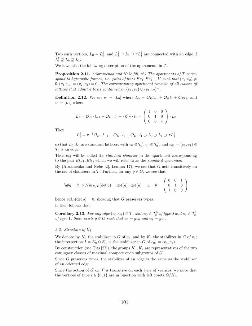
Two such vertices, L0 = L]0, and L]1 ⊇ L1 ⊇ πL]1 are connected with an edge if

L]1 ⊇ L0 ⊇ L1.We have also the following description of the apartments in T .

Proposition 2.11. (Abramenko and Nebe [2], §6) The apartments of T corre-spond to hyperbolic frames, i.e. pairs of lines Ev1, Ev2 ⊂ V such that (v1, v2) 6=0, (v1, v1) = (v2, v2) = 0. The corresponding apartment consists of all classes oflattices that admit a basis contained in {v1, v2} ∪ 〈v1, v2〉⊥.

Definition 2.12. We set v0 = [L0] where L0 = OEl−1 + OEl0 + OEl1, andv1 = [L1] where

L1 = OE · l−1 +OE · l0 + πOE · l1 =

1 0 00 1 00 0 π

· L0

ThenL]1 = π−1OE · l−1 +OE · l0 +OE · l1 ⊃ L0 ⊃ L1 ⊃ πL]1

so that L0, L1 are standard lattices, with v0 ∈ T 00 , v1 ∈ T 1

0 , and e01 = (v0, v1) ∈T1 is an edge.Then e01 will be called the standard chamber in the apartment correspondingto the pair El−1, El1, which we will refer to as the standard apartment.By (Abramenko and Nebe [2], Lemma 17), we see that G acts transitively onthe set of chambers in T . Further, for any g ∈ G, we see that

tgθg = θ ⇒ NmE/F (det g) = det(g) · det(g) = 1, θ =

0 0 10 1 01 0 0

hence valE(det g) = 0, showing that G preserves types.It then follows that

Corollary 2.13. For any edge (u0, u1) ∈ T , with u0 ∈ T 00 of type 0 and u1 ∈ T 1

0

of type 1, there exists g ∈ G such that u0 = gv0 and u1 = gv1.

2.2. Structure of U3

We denote by K0 the stabilizer in G of v0, and by K1 the stabilizer in G of v1;the intersection I = K0 ∩K1 is the stabilizer in G of e01 = (v0, v1).By construction (see Tits [27]), the groups K0,K1 are representatives of the twoconjugacy classes of maximal compact open subgroups of G.Since G preserves types, the stabilizer of an edge is the same as the stabilizerof an oriented edge.Since the action of G on T is transitive on each type of vertices, we note thatthe vertices of type i ∈ {0, 1} are in bijection with left cosets G/Ki.

101

Proposition 2.14. Representing the elements of G in the basis l−1, l0, l1, wehave

K0 = GL3(OE) ∩G, K1 =

OE OE π−1OEpE OE OEpE pE OE

∩G

K0 ∩K1 = I =

OE OE OEpE OE OEpE pE OE

∩G

Proof. Let g ∈ K0. Recall that L0 = OEl−1 +OEl0 +OEl1. Then, as [gL0] =[L0], and det(g) ∈ O×E , we must have gL0 = L0, whence gl−1, gl0, gl1 ∈ L0 =OEl−1 +OEl0 +OEl1.It follows that g ∈ M3(OE). Since g ∈ G ⊂ GL3(E) and g−1L0 = L0, bysymmetry we see that g ∈ GL3(OE)∩G. Conversely, if g ∈ GL3(OE)∩G, thenclearly gl−1, gl0, gl1 ∈ L0 , showing that gL0 ⊂ L0, and as g ∈ GL3(OE), we seethat g−1 ∈ GL3(OE) ∩ G, hence g−1L0 ⊂ L0, so L0 ⊂ gL0, showing equality.Therefore K0 = GL3(OE) ∩G.Next, let g ∈ K1. Since [gL1] = [L1] and det(g) ∈ O×E , we must have gL1 = L1

and furthermore gL]1 = L]1.

As L1 =

1 0 00 1 00 0 π

· L0, we see that L]1 =

π−1 0 00 1 00 0 1

· L0, and, with

the obvious definitions of g−1, g1,

g1L0 =

1 0 00 1 00 0 π−1

g

1 0 00 1 00 0 π

L0 = L0

g−1L0 =

π 0 00 1 00 0 1

g

π−1 0 00 1 00 0 1

L0 = L0

showing that g1, g−1 ∈ K0, whence

g ∈

1 0 00 1 00 0 π

K0

1 0 00 1 00 0 π−1

∩

π−1 0 00 1 00 0 1

K0

π 0 00 1 00 0 1

=

=

OE OE π−1OEOE OE π−1OEpE pE OE

∩

OE π−1OE π−1OEpE OE OEpE OE OE

∩G =

=


∩G

102

Conversely, if g ∈


∩G, then g1, g−1, defined as above,

satisfy g1, g−1 ∈ K0,hence g1L0 = L0, g−1L0 = L0, showing that gL1 = L1 and gL]1 = L]1.

The following proposition is a special case of (Tits [27], 3.3.3). It follows fromthe fact that Ki acts transitively on the vertices at distance 2n from vi.

Proposition 2.15. (Cartan decomposition) If we denote α =

π−1 0 00 1 00 0 π

,

and let i ∈ {0, 1} thenG =

∐

n∈Z≥0

Kiα−nKi.

The following proposition is a special case of (Tits [27], 3.3.1), but since ourcase is much simpler, we prove it directly.

Proposition 2.16. (Iwahori decomposition) We have

K0 = I∐

IsI, K1 = I∐

IβI

where

s =

0 0 10 1 01 0 0

, β = αs =

0 0 π−1

0 1 0π 0 0

.

Proof. If E/F is unramified, consider the natural reduction map ρ0 : K0 =GL3(OE) ∩ G → G(kF ) defined by reducing the entries modulo π. ThenI = ρ−1

0 (B(kF )) is the preimage of the parabolic subgroup of upper triangularmatrices over the residue field, and considering the Bruhat decomposition overthe residue field, we see that

G(kF ) = B(kF )∐

B(kF )sB(kF )

Taking preimages under ρ0, we see that

K0 = GL3(OE) ∩G = ρ−10 (G(kF )) = I

∐IsI

For K1, we consider the group

H(kF ) =

a 0 b0 c 0d 0 e

| c ∈ k1

E , ad, be ∈ k−E , ae+ db = 1

≤ G(kF )

where k−E = {x ∈ kE | x+ x = 0} and k1E = {x ∈ kE | x · x = 1}.

103

Consider the natural reduction map ρ1 : K1 → H(kF ) defined by

ρ1

a b π−1cπd e fπg πh i

=

a 0 c0 e 0g 0 i

mod π

Then I = ρ−11 (BH(kF )) where BH(kF ) ⊂ H(kF ) is the parabolic subgroup

of lower triangular matrices in H. Considering the Bruhat decomposition ofH(kF ) we see that

H(kF ) = BH(kF )∐

BH(kF )sBH(kF )

Taking preimages under ρ1, we see that

K1 = ρ−11 (H(kF )) = I

∐Iρ−1

1 (s)I = I∐

IβI

If E/F is ramified, we consider similarly the natural reductions ρ0 : K0 →O3(kF ) and ρ1 : K1 → H′(kF ), where

O3(kF ) = {g ∈ GL3(kF ) | tgθg = θ}

and

H′(kF ) =

a 0 b0 ±1 0c 0 d

| ad− bc = 1

≤ O3(kF )

Letting B′(kF ) ≤ O3(kF ) and B′H(kF ) ≤ H′(kF ) be the parabolic subgroupsof upper and lower triangular matrices, respectively, over the residue field, wemay consider the Bruhat decompositions of O3(kF ) and H ′(kF ) to obtain

O3(kF ) = B′(kF )∐

B′(kF )sB′(kF ), H′(kF ) = B′H(kF )

∐B′H(kF )sB

′H(kF )

Again, I = ρ−10 (B′(kF )) = ρ−1

1 (B′H(kF )) so taking preimages we obtain the

required result.

The geometric meaning is that the stabilizer of an edge e = (o(e), t(e)) ∈ T1

acts transitively on the remaining edges starting at o(e).Let N be the unipotent radical of G. Then N = N(F ) is given by

N =

nb,z :=

1 b z

0 1 −b0 0 1

| b, z ∈ E, z + z + bb = 0

The following is a consequence of (Tits [27] 1.15 and 3.5, see also Bruhat andTits [7] 4.4), but as in this specific case, it is much simpler, we provide a straight-forward proof.

104

Lemma 2.17. (Iwasawa decomposition) One has G = BK0 = BK1.

Proof. First note, by the Bruhat decomposition, that G = B∐BsN , hence it

is enough to show that for any n ∈ N , sn ∈ BK0 ∩BK1.Let n = nb,z ∈ N . If z ∈ OE , then bb = −z − z ∈ OE ∩ F = OF , hence b ∈ OE .In that case, note that

sn =

0 0 1

0 1 −b1 b z

=

π 0 00 1 00 0 π−1

·

0 0 π−1

0 1 −bπ πb πz

∈ BK1 ∩K0

Else, we have z−1 ∈ pE and as bb = −z − z, also z−1b, z−1b ∈ pE . In this case,we note that

sn =

0 0 1

0 1 −b1 b z

=

z−1 z−1b 1

0 1 −b0 0 z

·

1 0 0

z−1b −z−1z 0z−1 z−1b 1

∈ BK0∩BK1

For later use, we shall need a decomposition of G to left cosets of K0. For thatwe introduce some notation.Let N0 = N(OF ) = {nb,z ∈ N | b, z ∈ OE}, and for any r ∈ N,

N2r = {nb,z ∈ N | b ∈ πrOE , z ∈ π2rOE}

andN2r−1 = {nb,z ∈ N | b ∈ πrOE , z ∈ π2r−1OE}.

Further, for any r ∈ N, denote Nr = sNrs for the filtration on the oppositeunipotent radical. We then have

Proposition 2.18. For any n ≥ 0, let Rn be a system of representatives forN0/N2n, and for n ≥ 1 let Rn be a system of representatives for N1/N2n. Then

G =

∐

η∈Rn,n≥0

ηα−nK0

∐

∐

η∈Rn+1,n≥0

ηβα−nK0

where

α =

π−1 0 00 1 00 0 π

, β = αs =

0 0 π−1

0 1 0π 0 0

Proof. We have a Cartan decomposition G =∐n≥0K0α

−nK0 and a Iwahoridecomposition K0 = I

∐IsI. Let e be an edge in T , say connecting u0 to

u1. Then there exists a unique edge e′ in the standard apartment of T such

105

that the couple (e01, e) is G-equivalent to (e01, e′). Since e01 is fixed, they are

I-equivalent. More generally, we denote the vertices in the standard apartmentby (vn)n∈Z, and let eij = (vi, vj) for any i, j such that |i− j| = 1.It follows that the edges {e2n,2n+1, e2n+2,2n+1}n∈Z form a set of representativesfor I\T1

∼= I\G/I. Moreover, e2n,2n+1 = αne0,1 and e2n+2,2n+1 = αne2,1 =αnβe0,1. It follows that a set of representatives for the double cosets I\G/I isgiven by {αn, βαn}n∈Z.As αn+1K0 = βα−nK0 we see that in the decomposition

G =

∐

n≥0

Iα−nK0

∐

∐

n≥0

Iβα−nK0

the RHS indeed coversG. To see that the union is disjoint, note that Iα−nK0/K0

corresponds by action of I on α−nv0 to vertices at distance 2n from v0, whichare also at distance 2n+ 1 from v1 (i.e. the geodesic from v0 to them does notpass through v1). However, we know that the stabilizer of α−nv0 is α−nK0α

n.It follows that these vertices correspond bijectively to cosets I/I ∩ α−nK0α

n.Similarly, Iβα−nK0/K0 corresponds by action of I on βα−nv0 to vertices atdistance 2(n + 1) from v0, which are also at distance 2n + 1 from v1(i.e. thegeodesic from v0 to them passes through v1). However, we know that the sta-bilizer of βα−nv0 is βα−nK0α

nβ−1. It follows that these vertices correspondbijectively to cosets I/I ∩ βα−nK0α

nβ−1.Computation shows that

α−nK0αn ∩ I =

OE πnOE π2nOEπOE OE πnOEπOE πOE OE

∩G

βα−nK0αnβ−1 ∩ I =

OE OE OEπn+1OE OE OEπ2n+2OE πn+1OE OE

∩G

hence, the natural quotient maps N0 ↪→ I, N1 ↪→ I induce isomorphisms

I/α−nK0αn∩I ' N0/N2n, I/βα−nK0α

nβ−1∩I ' N1/N2n+2

Consequently, the proposition follows.

By the proof above, we see that in fact, considering only vertices of distance 2from v0, we get the following corollary:

Corollary 2.19. Let R1, R1 be as above. Then

K0α−1K0 = Iα−1K0

∐IβK0 =

∐

η∈R1

ηα−1K0

∐

∐

η∈R1

ηβK0

106

We also introduce a definition of “spheres” around the vertex v0.

Definition 2.20. For any 0 ≤ n ∈ Z, we let

S0n = Iα−nK0 =

∐

η∈Rnηα−nK0, S1

n+1 = Iβα−nK0 =∐

η∈Rn+1

ηβα−nK0

Let S0 = S00 , and for any n ∈ N, let Sn = S0

n

∐S1n = K0α

−nK0. Further,denote Bn =

∐ni=0 Si.

Remark 2.21. We note that Sn/K0 corresponds to the collection of vertices ofdistance 2n from v0, and that Bn/K0 corresponds to the collection of all verticesof type 0 of distance at most 2n from v0.

2.3. Filtrations on the stabilizers

We will define certain decreasing filtrations on the stabilizers defined above -I,K0 and K1, by normal subgroups which are compact open in G.We follow the construction described in (Schneider and Stuhler [21]), of filtra-tions on the stablilizers, and specialize it to our case, with G = U3(F ).It follows that we may define for each e ≥ 1 the subgroups

I(e) =

1 + πeOE πe−1OE πe−1OEπeOE 1 + πeOE πe−1OEπeOE πeOE 1 + πeOE

∩G

K0(e) =

1 + πeOE πeOE πeOEπeOE 1 + πeOE πeOEπeOE πeOE 1 + πeOE

∩G

K1(e) =

1 + πeOE πe−1OE πe−1OEπeOE 1 + πeOE πe−1OEπe+1OE πeOE 1 + πeOE

∩G

which are normal in I,K0,K1, respectively and compact open in G. In partic-ular, we see that

K0(1) =

U1E pE pE

pE U1E pE

pE pE U1E

∩G

I(1) =

U1E OE OE

pE U1E OE

pE pE U1E

∩G

and

K1(1) =

U1E OE OE

pE U1E OE

p2E pE U1

E

∩G

107

where U1E = 1 + pE .

These filtrations play a role in the main theorem in (Schneider and Stuhler [21],II.3.1), which allows us to interpret a representation as the 0-th homology of acoefficient system.Remark 2.22. One could also define the filtration corresponding to a facet σ byletting U (e)

σ be the stabilizer of all vertices which are at distance at most e fromσ.In particular, for i = 0, 1, Ki(1) is the stabilizer of the star pointed at vi , andI(1) is the stabilizer of all triangles containing e01 as an edge. However, we willnot use this description.

2.4. Lemmata on Finite fields

In what follows, p is a prime number, q is a power of p, and Fq is the uniquefield containing q elements.G(Fq) = U3(Fq) is the unitary group in three variables over Fq, i.e. U3(Fq) ={g ∈ GL3(Fq2) | t

gsg = s}, and F−q2 = {x ∈ Fq2 | x+ xq = 0}.We further let B(Fq) be the Borel subgroup of upper triangular matrices, andN(Fq) its unipotent radical. As before, we see that

N(Fq) =

nb,z =

1 b z0 1 −bq0 0 1

| b, z ∈ Fq2 , z + zq + bq+1 = 0

In addition, we consider O3(Fq) = {g ∈ GL3(Fq) |t gsg = s}, and its unipotentradical N′(Fq), which is given by

N′(Fq) =

nb.z =

1 b z0 1 −b0 0 1

| b, z ∈ Fq, 2z + b2 = 0

Lemma 2.23. For any q, one has

|N(Fq)| = q3, |F−q2 | = q, |N′(Fq)| = q

Moreover, for any 0 6= i ∈ F−q2 , F−q2 = Fq · i, and if p = 2, then F−q2 = Fq.

Proof. Assume that p 6= 2, and let α ∈ F×q2 be a generator, then αq+1 ∈ F×q isnot a square in Fq, as q+1

2 ∈ Z and(αq+1

2

)q−1

= αq2−1

2 = −1

so that αq+1

2 /∈ Fq. Further, we have(αq+1

2

)q= α

q(q+1)2 = −α q+1

2

108

so that, denoting i = αq+1

2 , we see that i = −i. As i /∈ Fq, {1, i} is a basis forFq2 over Fq, and for any b, z ∈ Fq2 we may write b = b1 + b2i, z = z1 + z2i, withb1, b2, z1, z2 ∈ Fq so that nb,z ∈ N(Fq) if and only if

2z1 = −(b21 − b22i2) ⇐⇒ z1 = −b21 − b22i2

2

Note that 2 is invertible in Fq, so this makes sense. It follows, that given b, z1 isuniquely determined, and z2 can attain any value. It follows that |N(Fq)| = q3

and∣∣∣F−q2

∣∣∣ = q.

Similarly, as 2 is invertible in Fq, N′(Fq) = {nb,−b2/2 | b ∈ Fq} is in bijectionwith Fq, hence |N′(Fq)| = q.If p = 2, we see that zq = −z ⇐⇒ zq = z, hence F−q2 = Fq, and we still have∣∣∣F−q2

∣∣∣ = |Fq| = q, and for some α ∈ Fq2\Fq, {1, α} is a basis for Fq2 over Fq, andfor any b, z ∈ Fq2 we may write b = b1 +b2α, z = z1 +z2α, with b1, b2, z1, z2 ∈ Fqso that nb,z ∈ N(Fq) if and only if

(α+ αq) · z2 = b21 + b22αq+1b22 + b1b2(α+ αq) ⇐⇒ z2 =

b21 + b22 · αq+1

α+ αq+ b1b2

Since α /∈ Fq, α 6= αq, hence α + αq 6= 0 is invertible, and z2 is uniquely welldefined for any b1, b2. z1 is determined arbitrarily, hence again |N(Fq)| = q3.Also, N′(Fq) = {nb,z | b = 0, z ∈ Fq} = {n0,z | z ∈ Fq} is again in bijection withFq, hence |N′(Fq)| = q.

The following lemma is a consequence, which will be used in Section 7, in thecourse of the proof of the main theorem.

Lemma 2.24. (a) Let 1 6= η : F×q2 → C be a character. Extend it to Fq2 bysetting η(0) = 0. Then for any 0 6= i ∈ F−q2 , one has

∑

z∈F−q2

η(z) =

0 η �F×q 6= 1

(q − 1)η(i) η �F×q = 1, p 6= 2

q − 1 η �F×q = 1, p = 2

and

∑

nb,z∈N(Fq)η(z) =

0 η �F×q 6= 1

−q(q − 1)η(i) η �F×q = 1, p 6= 2, η 6= 1

−q(q − 1) η �F×q = 1, p = 2, η 6= 1

q3 − 1 η = 1

(b) Let p 6= 2 and letη : F×q → C be a character. Extend it to Fq by settingη(0) = 0. Then

∑

b∈Fqη

(−b

2

2

)=

{0 η 6= εq, 1

η(− 1

2

)· (q − 1) η = εq, 1

109

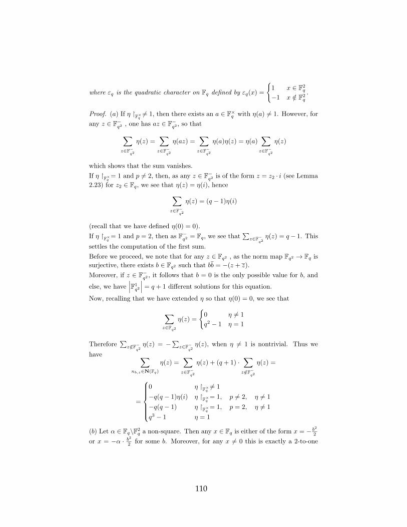
where εq is the quadratic character on Fq defined by εq(x) =

{1 x ∈ F2

q

−1 x /∈ F2q

.

Proof. (a) If η �F×q 6= 1, then there exists an a ∈ F×q with η(a) 6= 1. However, forany z ∈ F−q2 , one has az ∈ F−q2 , so that

∑

z∈F−q2

η(z) =∑

z∈F−q2

η(az) =∑

z∈F−q2

η(a)η(z) = η(a)∑

z∈F−q2

η(z)

which shows that the sum vanishes.If η �F×q = 1 and p 6= 2, then, as any z ∈ F−q2 is of the form z = z2 · i (see Lemma2.23) for z2 ∈ Fq, we see that η(z) = η(i), hence

∑

z∈F−q2

η(z) = (q − 1)η(i)

(recall that we have defined η(0) = 0).If η �F×q = 1 and p = 2, then as F−q2 = Fq, we see that

∑z∈F−

q2η(z) = q− 1. This

settles the computation of the first sum.Before we proceed, we note that for any z ∈ Fq2 , as the norm map Fq2 → Fq issurjective, there exists b ∈ Fq2 such that bb = −(z + z).Moreover, if z ∈ F−q2 , it follows that b = 0 is the only possible value for b, and

else, we have∣∣∣F1q2

∣∣∣ = q + 1 different solutions for this equation.

Now, recalling that we have extended η so that η(0) = 0, we see that

∑

z∈Fq2η(z) =

{0 η 6= 1

q2 − 1 η = 1

Therefore∑z/∈F−

q2η(z) = −∑z∈F−

q2η(z), when η 6= 1 is nontrivial. Thus we

have ∑

nb,z∈N(Fq)η(z) =

∑

z∈F−q2

η(z) + (q + 1) ·∑

z/∈F−q2

η(z) =

=

0 η �F×q 6= 1

−q(q − 1)η(i) η �F×q = 1, p 6= 2, η 6= 1

−q(q − 1) η �F×q = 1, p = 2, η 6= 1

q3 − 1 η = 1

(b) Let α ∈ Fq\F2q a non-square. Then any x ∈ Fq is either of the form x = − b22

or x = −α · b22 for some b. Moreover, for any x 6= 0 this is exactly a 2-to-one

110

map, with ±b giving x, and for x = 0, we have b = 0 in both forms, hence ifη 6= 1

0 = 2 ·∑

x∈Fqη(x) =

∑

b∈Fqη

(−b

2

2

)+∑

b∈Fqη

(−α · b

2

2

)= (1 + η(α)) ·

∑

b∈Fqη

(−b

2

2

)

If η 6= εq, then there exists such α with η(α) 6= −1 , hence the sum vanishes.

Corollary 2.25. If E/F is unramified (so that q = q2F and f is even), then

T is bihomogeneous with degrees q3/2 + 1 and q1/2 + 1 for vertices of types 0,1respectively. If E/F is ramified, then T is homogeneous of degree q + 1, whereq = qE is the cardinality of the residue field of E.

Proof. By the identification of vertices of the tree with (G/K0)∐

(G/K1), wesee that the vertices of each type have the same degree. We note that K0K1 =K1

∐Iα−1K1 and K1K0 = K0

∐IβK0.

Indeed, as each Ki acts transitively on the neighbours of vi, it follows from theIwasawa decomposition (Corollary 2.19). We thus see that these decompositionsto left cosets of K1 and K0 correspond to the degrees of v0, v1, respectively.

In particular, as K1K0 = K0

∐(∐η∈R1

ηβK0

), we see that the degree of type

1 vertices, d1, is∣∣R1

∣∣+ 1 =∣∣N1/N2

∣∣+ 1.To obtain the result for type 0 vertices, we must decompose Iα−1K1 to leftcosets of K1 in a similar manner, and obtain that I/I∩α−1K1α'N0/N1, hence thedegree of type 0 vertices, d0, is |N0/N1|+ 1.Assume first that E/F is unramified. In this case, we may take π ∈ F , so thatπ = π. Here and in what follows, nb,z = snb,zs.Consider first the homomorphism N1 → k−E = {x ∈ kE | x + xqF = 0} definedby nb,z 7→ (π−1z) mod π. This is well defined, since for nb,z ∈ N1, z ∈ πOE ,whence π−1z ∈ OE , and as z + z + bb = 0, with bb ∈ π2OE , we see thatπ−1z+π−1z ∈ πOE , so that (π−1z) mod π ∈ k−E . This is also a homomorphismsince

nb,z · nc,y = nb+c,y+z−bc 7→ (π−1(y + z)) mod π

as bc ∈ π2OE for all nb,z, nc,y ∈ N1. Further, , if nb,z ∈ N2 then z ∈ π2OE ,so that π−1z mod π = 0, showing that the map factors through N2. As this isprecisely the kernel, we have an injective homomorphism N1/N2 → k−E .This map is bijective - indeed, if α ∈ k−E , choose a ∈ OF such that a mod π =Nm(α). Then the polynomial x2 +a ∈ OF [x] ⊂ OE [x] has a root when reducedmod π, namely α. Therefore, by Hensel’s Lemma, it has also a root z ∈ OEsuch that z mod π = α. It follows that z + z = 0, hence z ∈ E− = {x ∈ E |x+ x = 0}. Now n0,πz ∈ N1 maps to α.Now, by Lemma 2.23,

∣∣k−E∣∣ = qF = q1/2, showing that d1 = q1/2 + 1.

For d0, consider the reduction map N0 → N(kF ). It is a homomorphism withkernel N1, hence N0/N1 ' N(kF ). As, by Lemma 2.23, |N(kF )| = q3/2, we seethat d0 = q3/2 + 1.

111

Next, consider the case when E/F is ramified.We now have a homomorphism N1 → kE = kF defined by nb,z 7→ (π−1z)mod π. It is well defined, since for nb,z ∈ N1, z ∈ πOE , hence π−1z ∈ OE .It is also a homomorphism with kernel N2, by the same reasoning as in theunramified case. Finally, if α ∈ kE = kF , we may lift it to some z ∈ F suchthat z mod π = α, and then z = z. Choosing π such that π2 ∈ F , we see thatπ = −π, hence πz = −πz, so that n0,πz ∈ N1 maps to α, showing surjectivity.It follows that d1 = |kE |+ 1 = q + 1.For d0, consider the reduction map N0 → N′(Fq). It is a homomorphism withkernel N1, hence N0/N1 ' N′(kF ). As, by Lemma 2.23, |N′(kF )| = q, we seethat d0 = q + 1.

3. Representations of U3(F )

3.1. Qp-algebraic representations of U3(F )

As before, let C be a finite extension of Qp, containing E, such that

|Homalg(E,C)| = [E : Qp].

For 0 ≤ a, b ∈ Z, denote S(a, b) = SymaC3 ⊗ Symb(C3)?. If a, b ≥ 1 one has anatural contraction map ιa,b : S(a, b)→ S(a− 1, b− 1) defined by

ιa,b (x1x2 · · ·xa ⊗ y1y2 · · · yb) =a∑

i=1

b∑

j=1

〈xi, yj〉 (x1x2 · · · xi · · ·xa⊗y1y2 · · · yj · · · yb)

Denote its kernel by V (a, b). If ab = 0, we let V (a, b) = S(a, b).For τ ∈ Homalg(E,C), dτ ∈ Z and 0 ≤ aτ , bτ ∈ Z, we denote by ρ(aτ , bτ , dτ )τ

the irreducible algebraic representation of U3 ⊗F,τ C of highest weight

χτ : g = diag(z1, z2, z−11 ) 7→ τ(z1)aτ τ(z1)bτ · τ(det(g))dτ

with respect to B.We identify ρ(aτ , bτ , dτ )τ with a representation of G on the C-vector spaceV (aτ , bτ ), as follows.By choosing a basis (xτ,1, xτ,2, xτ,3) for (C3)?, and a dual basis (yτ,1, yτ,2, yτ,3)for C3 = ((C3)?)?, we may identify SymaC3 with the space of homogeneouspolynomials of degree a in the xτ,k, and similarly identify Symb(C3)? with thespace of homogeneous polynomials of degree b in the yτ,k.Under this identification, S(aτ , bτ ) is identified with the space of (aτ , bτ )-bihomogeneouspolynomials in the xτ,k, yτ,k. Explicitly,

S(aτ , bτ ) =⊕

i,j∈Z3≥0

|i|=aτ ,|j|=bτ

C · xiτyjτ

112

where xτ = (xτ,1, xτ,2, xτ,3), yτ = (yτ,1, yτ,2, yτ,3), i = (i1, i2, i3), j = (j1, j2, j3)are such that |i| = i1 + i2 + i3 = aτ , |j| = j1 + j2 + j3 = bτ , and we denotexiτ = xi1τ,1x

i2τ,2x

i3τ,3 and yjτ = yj1τ,1y

j2τ,2y

j3τ,3.

As 〈xτ,k, yτ,l〉 = δkl, the map ιa,b now takes the following form

ιaτ ,bτ(xiτy

jτ

)= ιaτ ,bτ

(xi1τ,1x

i2τ,2x

i3τ,3 ⊗ yj1τ,1yj2τ,2yj3τ,3

)=

=3∑

k=1

3∑

l=1

ik∑

r=1

jl∑

s=1

〈xτ,k, yτ,l〉(x−1τ,k · xiτ ⊗ y−1

τ,l · yjτ)

=

=3∑

k=1

ikjkx−1τ,ky

−1τ,k · xiτyjτ =

(3∑

k=1

∂2

∂xτ,k∂yτ,k

)(xiτy

jτ

)

Therefore, we have

V (aτ , bτ ) =

{f(xτ , yτ ) ∈ S(aτ , bτ ) |

3∑

k=1

∂2f

∂xτ,k∂yτ,k= 0

}

This is the space of bihomogeneous polynomials of bidegree (aτ , bτ ) with coef-ficients in C satisfying a certain differential equation. G acts on it as follows-Any τ : E ↪→ C induces an embedding, which we denote by the same letterτ : GL3(E)→ GL3(C), as there is no risk of confusion.GL3(C) acts on C3 naturally, hence for any τ we obtain a natural G = U3(F ) ⊂GL3(E) action, which we denote by (g, v) 7→ τ(g) · v.This action also induces a natural right action on (C3)?, namely (v? ·τ(g))(v) =v?(τ(g) · v) for any v ∈ (C3)?, v ∈ C3.Therefore it induces an action on S(aτ , bτ ) defined by

(g · f)(xτ , yτ ) = τ(det(g))dτ · f(xτ · τ(g), τ(g)−1 · yτ )

Note that ιaτ ,bτ commutes with this action of G. Indeed, writing for simplicityg for τ(g), and x, y, a, b, d for xτ , yτ , aτ , bτ , dτ we obtain

ιa,b(g · f)(x, y) =3∑

k=1

∂2(g · f)

∂xk∂yk(x, y) =

3∑

k=1

∂

∂yk

(∂(g · f)

∂xk

)(x, y) =

= det(g)d ·3∑

k=1

∂

∂yk

3∑

j=1

gkj ·∂f

∂xj(x · g, g−1y)

=

= det(g)d ·3∑

k=1

3∑

l=1

(g−1)lk

3∑

j=1

gkj ·∂2f

∂xj∂yl(x · g, g−1y)

113

But∑3k=1(g−1)lkgkj = δlj , by definition, so that

ιa,b(g · f)(x, y) = det(g)d ·3∑

l=1

∂2f

∂xl∂yl(x · g, g−1y) = g · (ιa,b(f))(x, y)

Therefore V (aτ , bτ ) = ker ιaτ ,bτ ⊆ S(aτ , bτ ) is a subrepresentation with theinduced action.This representation of G is a realization of ρ(aτ , bτ , dτ )τ , with xaτ,1ybτ,3 the high-est weight vector, and xaτ,3ybτ,1 the lowest weight vector, with respect to B andM . If vτ ∈ ρ(aτ , bτ , dτ )τ and g ∈ G, we will denote simply by gvτ the action ofg on vτ .Fix a = (aτ )τ :E↪→C , b = (bτ )τ :E↪→C and d = (dτ )τ :E↪→C such that aτ , bτ ≥ 0.Denote by ρa,b,d the representation of G on the underlying vector space

ρ(a, b, d) =⊗

τ :E↪→Cρ(aτ , bτ , dτ )τ

for which an element g ∈ G acts componentwise.In particular, for any

⊗τ :E↪→C vτ ∈ ρ(a, b, d),

ρa,b,d(g)

( ⊗

τ :E↪→Cvτ

)=

⊗

τ :E↪→Cgvτ .

For i = (iτ ), j = (jτ ) sequences of iτ , jτ ∈ Z3≥0 with |iτ | = aτ , |jτ | = bτ , we

denotexiyj =

⊗

τ :E↪→Cxiττ y

jττ

The representations ρa,b,d are irreducible, and in fact exhaust all irreduciblealgebraic representations of G = U3(F ).This description of the irreducible algebraic representations of GL3 is given e.g.in (Fulton and Harris [12]) over C, and the consequence for representations ofU3 over C can be obtained, for example, by considering (Tits [26]).Note that this description, up to a twist by a power of the determinant, exhaustsall irreducible algebraic representations of G over C.For any τ : E ↪→ C, we may consider an endomorphism Uaτ ,bτ ∈ End(S(aτ , bτ ))whose action is described by

Uaτ ,bτ (xiτyjτ ) = τ(π)i1−j1+aτ · τ(π)j3−i3+bτ · xiτyjτ

for any i, j ∈ Z3≥0 such that |i| = aτ , |j| = bτ .

DenoteUa,b,d =

⊗

τ :E↪→CUaτ ,bτ ,dτ (3.1)

114

Lemma 3.1. There exists a unique function ψ : G → EndC (ρ(a, b, d)) sup-ported in K0α

−1K0 such that:(i) for all k1, k2 ∈ K0, we have ψ(k1αk2) = ρa,b,d(k1) ◦ ψ(α−1) ◦ ρa,b,d(k2).(ii) ψ(α−1) = Ua,b,d.

Proof. Suppose there exist two such functions ψ1, ψ2. Then by (ii), ψ1(α−1) =ψ2(α−1), hence by (i), ψ1(g) = ψ2(g) for all g ∈ K0α

−1K0, hence the unique-ness.For the existence, it suffices to show that ψ is well defined, i.e. that if k1α

−1k2 =α−1 with k1, k2 ∈ K0, then ψ(k1α

−1k2) = ψ(α−1).But for any i = (iτ )τ :E↪→C and j = (jτ )τ :E↪→C with iτ , jτ ∈ Z3

≥0 such that|iτ | = aτ and |jτ | = bτ , one has

Ua,b,d =⊗

τ :E↪→CUaτ ,bτ ,dτ =

( ∏

τ :E↪→Cτ(π)aτ+dτ · τ(π)bτ−dτ

)· ρa,b,d(α−1) (3.2)

For brevity, denote

πa,b,d =

( ∏

τ :E↪→Cτ(π)aτ+dτ · τ(π)bτ−dτ

)

Therefore, if k1α−1k2 = α−1 for some k1, k2 ∈ K0, then

ρa,b,d(k1) ◦ πa,b,d · ρa,b,d(α−1) ◦ ρa,b,d(k2) = πa,b,d · ρa,b,d(α−1)

henceρa,b,d(k1) ◦ ψ(α−1) ◦ ρa,b,d(k2) = ψ(α−1)

which finishes the proof.

3.2. Compactly induced representationsIn what follows R is either C or OC .Definition 3.2. Let G be a topological group, and let H be a closed subgroup.Let (π, V ) be a R-linear representation of H over a free R-module of finite rankV . We denote by indGHπ or by indGHV the smooth compact induction of (π, V )from H to G. The space of the representation is

indGHπ =

{f : G→ V | f(hg) = π(h)f(g) ∀h ∈ H

f has compact support mod H, f is smooth

}

and G acts on indGHπ by right translation, i.e. (gf)(x) = f(xg) for all g, x ∈ G.IfG is topological group,H is a closed subgroup, and (π, V ) is anR-representationof H, we denote by [g, v] ∈ indGHπ the function supported on the coset Hg−1

with value v ∈ V at g−1. Explicitly

[g, v](x) =

{π(h)(v) x = hg−1

0 x /∈ Hg (3.3)

115

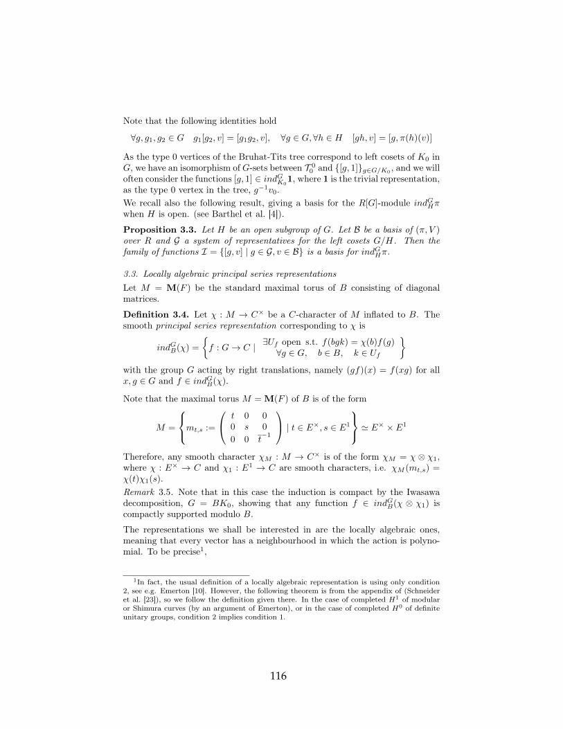
Note that the following identities hold

∀g, g1, g2 ∈ G g1[g2, v] = [g1g2, v], ∀g ∈ G,∀h ∈ H [gh, v] = [g, π(h)(v)]

As the type 0 vertices of the Bruhat-Tits tree correspond to left cosets of K0 inG, we have an isomorphism of G-sets between T 0

0 and {[g, 1]}g∈G/K0, and we will

often consider the functions [g, 1] ∈ indGK01, where 1 is the trivial representation,

as the type 0 vertex in the tree, g−1v0.We recall also the following result, giving a basis for the R[G]-module indGHπwhen H is open. (see Barthel et al. [4]).

Proposition 3.3. Let H be an open subgroup of G. Let B be a basis of (π, V )over R and G a system of representatives for the left cosets G/H. Then thefamily of functions I = {[g, v] | g ∈ G, v ∈ B} is a basis for indGHπ.

3.3. Locally algebraic principal series representationsLet M = M(F ) be the standard maximal torus of B consisting of diagonalmatrices.

Definition 3.4. Let χ : M → C× be a C-character of M inflated to B. Thesmooth principal series representation corresponding to χ is

indGB(χ) =

{f : G→ C | ∃Uf open s.t. f(bgk) = χ(b)f(g)

∀g ∈ G, b ∈ B, k ∈ Uf

}

with the group G acting by right translations, namely (gf)(x) = f(xg) for allx, g ∈ G and f ∈ indGB(χ).

Note that the maximal torus M = M(F ) of B is of the form

M =

mt,s :=

t 0 00 s 0

0 0 t−1

| t ∈ E×, s ∈ E1

' E

× × E1

Therefore, any smooth character χM : M → C× is of the form χM = χ ⊗ χ1,where χ : E× → C and χ1 : E1 → C are smooth characters, i.e. χM (mt,s) =χ(t)χ1(s).Remark 3.5. Note that in this case the induction is compact by the Iwasawadecomposition, G = BK0, showing that any function f ∈ indGB(χ ⊗ χ1) iscompactly supported modulo B.

The representations we shall be interested in are the locally algebraic ones,meaning that every vector has a neighbourhood in which the action is polyno-mial. To be precise1,

1In fact, the usual definition of a locally algebraic representation is using only condition2, see e.g. Emerton [10]. However, the following theorem is from the appendix of (Schneideret al. [23]), so we follow the definition given there. In the case of completed H1 of modularor Shimura curves (by an argument of Emerton), or in the case of completed H0 of definiteunitary groups, condition 2 implies condition 1.

116

Definition 3.6. A C-representation (π, V ) of G is called locally algebraic if:

1. The restriction of π to any compact open subgroup K of G is an algebraicdirect sum of finite dimensional irreducible representations of K.

2. For any vector v ∈ V , there exists a compact open subgroup Kv in G, anda finite dimensional subspace U of V , containing v, such that Kv leaves Uinvariant, and operates on U via restriction to Kv of a finite dimensionalalgebraic representation of G.

Definition 3.7. The locally algebraic C-representation of G, Vsm⊗Valg, whereVsm is a smooth representation, and Valg is an algebraic representation, is calleda locally algebraic principal series representation if Vsm is a smooth principalseries representation.

Recall the following result (see Appendix of (Schneider et al. [23]), Thm 1)about irreducibility of locally algebraic representations -

Theorem 3.8. Every irreducible locally algebraic representation π of G is thetensor product π = πalg ⊗ πsm of an irreducible algebraic representation πalgof G and a smooth irreducible algebraic representation πsm of G. Conversely,the tensor product πalg ⊗ πsm of an irreducible algebraic representation πalg ofG and an irreducible smooth representation πsm of G, is an irreducible locallyalgebraic representation of G.

As in this work, we are interested in irreducible locally algebraic representations,we will only consider representations of the form πalg ⊗ πsm. Furthermore, thecases where πsm is essentially discrete series or supercuspidal are known (seeSorensen [25]), hence we consider only the cases where πsm is an irreduciblesmooth principal series representation as above.We remark that the Breuil-Schneider conjecture also deals with indecomposablereducible representations, however we will not address this case presently.Thus, by the above classification of irreducible algebraic representations, we areinterested in representations of the form

(π, V ) = IndGB(χ⊗ χ1)⊗ ρa,b,d

where χ : E× → C, χ1 : E1 → C are smooth characters and a, b ∈ ZHomalg(E,C)≥0 .

3.4. Spherical Hecke algebras

Let R be either C or OC , let K be an open compact subgroup of G, and let ρ bea continuous R-linear representation of K over a free R-module Vρ of finite rank.The Hecke algebra Hρ(K,G) associated to K and ρ is the R-algebra defined by

Hρ(K,G) = EndR[G](indGKρ).

By Frobenius reciprocity for compact induction, for any R-representation π ofG, one has

HomR[G](indGKρ, π) ' HomR[K](ρ, π |K).

117

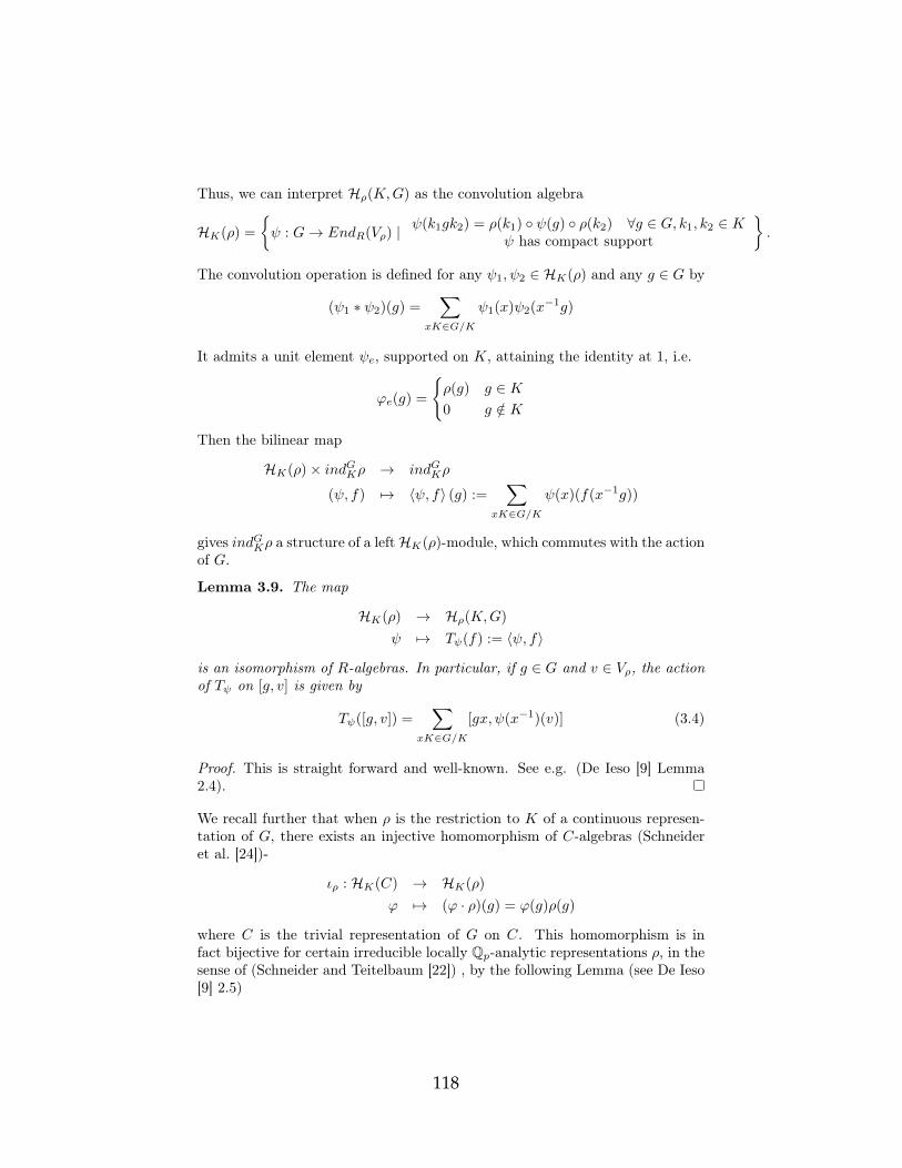
Thus, we can interpret Hρ(K,G) as the convolution algebra

HK(ρ) =

{ψ : G→ EndR(Vρ) | ψ(k1gk2) = ρ(k1) ◦ ψ(g) ◦ ρ(k2) ∀g ∈ G, k1, k2 ∈ K

ψ has compact support

}.

The convolution operation is defined for any ψ1, ψ2 ∈ HK(ρ) and any g ∈ G by

(ψ1 ∗ ψ2)(g) =∑

xK∈G/Kψ1(x)ψ2(x−1g)

It admits a unit element ψe, supported on K, attaining the identity at 1, i.e.

ϕe(g) =

{ρ(g) g ∈ K0 g /∈ K

Then the bilinear map

HK(ρ)× indGKρ → indGKρ

(ψ, f) 7→ 〈ψ, f〉 (g) :=∑

xK∈G/Kψ(x)(f(x−1g))

gives indGKρ a structure of a leftHK(ρ)-module, which commutes with the actionof G.

Lemma 3.9. The map

HK(ρ) → Hρ(K,G)

ψ 7→ Tψ(f) := 〈ψ, f〉

is an isomorphism of R-algebras. In particular, if g ∈ G and v ∈ Vρ, the actionof Tψ on [g, v] is given by

Tψ([g, v]) =∑

xK∈G/K[gx, ψ(x−1)(v)] (3.4)

Proof. This is straight forward and well-known. See e.g. (De Ieso [9] Lemma2.4).

We recall further that when ρ is the restriction to K of a continuous represen-tation of G, there exists an injective homomorphism of C-algebras (Schneideret al. [24])-

ιρ : HK(C) → HK(ρ)

ϕ 7→ (ϕ · ρ)(g) = ϕ(g)ρ(g)

where C is the trivial representation of G on C. This homomorphism is infact bijective for certain irreducible locally Qp-analytic representations ρ, in thesense of (Schneider and Teitelbaum [22]) , by the following Lemma (see De Ieso[9] 2.5)

118

Lemma 3.10. Let g = Lie(G). Then if the g ⊗Qp C-module Vρ is absolutelyirreducible, the map ιρ is bijective.

Recall that by Lemma 3.1, we have constructed ψ ∈ HK0(ρa,b) for any a, b ∈

ZHomalg(E,C)≥0 . By Lemma 3.9, it corresponds to a Hecke operator T ∈ Hρ(K0, G),

whose action on the elements [g, v] are given by the formula (3.4).

Lemma 3.11. There is a C-algebra isomorphism

Hρa,b,d(K0, G) ' C[T ]

Proof. The space Vρa,b,d is an absolutely irreducible g ⊗Qp C-module, henceιρa,b,d is an isomorphism of C-algebras. Lemma 3.9 shows that there exists aunique morphism of C-algebras uρa,b,d : HC(K0, G) → Hρa,b,d(K0, G) makingthe following diagram commute

HK0(C)∼ //

ιρa,b,d

��

HC(K0, G)

uρa,b,d

��HK0

(ρa,b,d)∼ // Hρa,b,d(K0, G)

(3.5)

By construction, this morphism is an isomorphism of C-algebras. Denote byT1 ∈ HC(K0, G) the element corresponding to 1K0α−1K0

∈ HK0(C) by Frobe-

nius reciprocity.If ϕ ∈ HK0

(C), then as it has compact support, by the Cartan decomposition(Proposition 2.15), it is supported on

∐ni=0K0α

−iK0 for some integer n. As ϕis K0-biinvariant (recall that C is the trivial representation), its restriction toeach Si = K0α

−iK0 is constant, hence we may write ϕ =∑ni=0 ϕi · 1K0α−iK0

.Let Ti ∈ HC(K0, G) be the operator corresponding to 1K0α−iK0

by Frobeniusreciprocity. Then we see that the Tn’s span HC(K0, G) over C. Geometrically,Tn is the operator associating to a vertex v of type 0 the sum of the vertices ofdistance 2n from v: this is because

1K0α−nK0=

∑

K0x∈K0\K0α−nK0

1K0x =

=∑

K0x∈K0\K0α−nK0

[x−1, 1] =∑

K0x∈K0\K0α−nK0

x−1 · [1, 1]

and then the x−1v0 are all distinct and give all vertices v′ ∈ T 00 such that v′ is

K0-equivalent to v2n. This means that (v0, v′) is equivalent to (v0, v2n), which

is precisely our assertion. From the geometrical description of Tn, one getsdirectly, using Corollary 2.25, that

T 21 =

{T2 + (q1/2 − 1)T1 + (q3/2 + 1)q1/2 E/F unramified

T2 + (q − 1)T1 + (q + 1)q E/F ramified

119

Explicitly, let d0, d1 be the degrees of vertices of types 0,1 respectively.If z is a vertex such that d(z, v) = 4, then there is a unique vertex w lying onthe geodesic from v to z with d(z, w) = 2 = d(v, w). Therefore, when applyingT 2

1 , each of them is counted once.If z is a vertex such that d(z, v) = 2, then there is a unique vertex u lying onthe geodesic from v to z, which is a common neighbour. This u has d1 − 2other neighbours whcih are at distance 2 from v, hence whem applying T 2

1 , it iscounted d1 − 2 times.Finally, v is counted once from every vertex of distance 2 from it. As there ared0 · (d1 − 1) such vertices, it is counted d0 · (d1 − 1) times.Since T 2

1 yields only vertices at distances 0, 2, 4 from v, these are all the possi-bilities, and we get

T 21 = T2 + (d1 − 2)T1 + d0 · (d1 − 1)

When we plug in the degrees in each of the cases, we get the answer.In any case, it follows that T2 ∈ C[T1]. Furthermore, for any n ≥ 3, we see that

T1Tn−1 =

{Tn + (q1/2 − 1)Tn−1 + q2Tn−2 E/F unramified

Tn + (q − 1)Tn−1 + q2Tn−2 E/F ramified

showing that if Tn−1 ∈ C[T1], then also Tn ∈ C[T1].Again, if we consider some vertex at distance 2n from v, there is a unique vertexat distance 2(n− 1) from v between them, which accounts for it when applyingT1Tn−1.If we consider a vertex at distance 2(n − 1) from v, there are d1 − 2 verticesof the same distance sharing a common neighbour with it, hence it is countedd1 − 2 times when applying T1Tn−1.Finally, if we have a vertex at distance 2(n−2) from v, there are (d0−1)(d1−1)vertices at distance 2(n − 1) from v, having this vertex on the geodesic, thuseach such vertex is counted (d0 − 1)(d1 − 1) times when applying T1Tn−1.When we plug in the degrees in each of the cases, we obtain the result.It follows that HC(K0, G) ' C[T1].As uρa,b,d(T1) = (πa,b,d)−1 · T , it follows that Hρa,b,d(K0, G) ' C[T ].

Finally, as described by Kato (Kato [17], Thm 3.2), we have an intimate con-nection between the Hecke algebra and the irreducible smooth principal seriesrepresentations.

Theorem 3.12. Let χ : M → C× be a smooth unramified character.Assume φ ∈ indGBχ is supported on BK0 and given there by φ(bk) = χ(b). Thenφ ∈

(indGBχ

)K0 .

120

Assume indGBχ is generated by φ. Define j : indGK0C → indGBχ by j(f) = Ff ,

whereFf (g) :=

∫

G

φ(gh−1)f(h)dh

Note: (i) Ff (bg) = χ(b)Ff (g)

(ii) Ff (g) =∑h∈K0\G φ(gh−1)f(h) = (f ∗ φ)(g)

Then j induces an isomorphism of G-representations

indGBχ 'indGK0

C

(T1 − αχ(T1)) · indGK0C

where αχ : HC(K0, G) → C is an algebra homomorphism of the Hecke algebrainduced by χ, and HC(K0, G) ' C[T1].

In particular, when indGBχ is irreducible, this holds. Thus, we obtain the fol-lowing corollary.

Corollary 3.13. Let χ : E× → C× be a smooth unramified character, and leta, b ∈ ZHomalg(E,C)

≥0 , d ∈ ZHomalg(E,C). Then if indGBχ is irreducible, one has

indGBχ⊗ ρa,b,d 'indGK0

ρa,b,d

(T − αχ(T )) · indGK0ρa,b,d

Proof. As ρa,b,d is a finite dimensional representation, tensoring with it is anexact functor, thus

indGBχ⊗ ρa,b,d '(indGK0

C)⊗ ρa,b,d(

(T1 − αχ(T1)) · indGK0C)⊗ ρa,b,d

However, by the commutative diagram (3.5), we see that(indGK0

C)⊗ ρa,b,d(

(T1 − αχ(T1)) · indGK0C)⊗ ρa,b,d

' indGK0ρa,b,d(

uρa,b,d(T1)− αχ(uρa,b,d(T1)))· indGK0

ρa,b,d

But, as uρa,b,d(T1) = (πa,b)−1 · T , the result follows.

In order to better understand the values of αχ(T1), we present the universalprincipal series.

3.5. The universal principal series

In this section, and in this section alone, R = C[t, t−1] where t is a variable, andlet χ : B → R× be the smooth character

χ

a ∗ ∗0 ∗ ∗0 0 a−1

= tvalE(a)

121

Note that these are not R and χ as they appear in previous sections.The universal unramified principal series representation is

π(χ) = indGBχ

Here valE : E× → Z is the normalized valuation on E such that valE(πE) = 1.Its specialization under t 7→ λ ∈ C× is π(χλ), the unramified principal seriesrepresentation.For any f ∈ π(χ), one may associate a locally-constant R-valued function f onN by the rule f(n) = f(sn).

Lemma 3.14. (i) This procedure identifies π(χ) with the space of locally con-stant functions on N satisfying

f(nb,z) = const · t−valE(z)

for all z large enough.

(ii) π(χ) is free of countable rank over R.

Proof. (i) We have

s ·

1 b z

0 1 −b0 0 1

=

z−1 −z−1b 1

0 −z−1z −b0 0 z

1 0 0

−z−1b 1 0z−1 z−1b 1

hence for large z, z−1b → 0, so one has f(nb,z) = t−valE(z) · f(1). By Bruhatdecomposition, this is reversible.Indeed, if F ∈ C∞(N) is a locally constant function satisfying F (nb,z) = c ·t−valE(z) for all z large enough, then we may define

fF (bsn) = χ(b) · F (n) ∀b ∈ B, n ∈ N

andfF (b) = χ(b) · c ∀b ∈ B

The function fF is well defined, since G = BsN∐B, with unique representa-

tives, by the Bruhat decomposition.Moreover, it is locally constant, as for g ∈ BsN it follows from the fact that Fis locally constant, and by the above equation

fF

1 0 0

−z−1b 1 0z−1 z−1b 1

= χ−1

z−1 −z−1b 1

0 −z−1z −b0 0 z

· F (nb,z)

so that for all z large enough,

fF

1 0 0

−z−1b 1 0z−1 z−1b 1

= tvalE(z) · c · t−valE(z) = c = fF (1)

122

This gives us an open compact neighbourhood of 1, such that fF is constantthere, and by translation, it shows that fF is locally constant on B.Finally, we note that fF (n) = fF (sn) = F (n) for all n ∈ N , and vice versa,

ff (bsn) = χ(b) · f(n) = χ(b) · f(sn) = f(bsn), ff (b) = χ(b) · f(1) = f(b)

showing that these are inverses.

Note that the functions f of compact support correspond to f vanishing on aneighbourhood of B.(ii) In this model, we see that π(χ) ∼= C∞c (N,R)⊕Rf0, where

f0(n) =

{1 n ∈ N(OE)

t−valE(z) n /∈ N(OE)

The space of locally constant function of compact support is easily seen to befree of countable rank.

3.5.1. Normed isotropic lines

Recall that B\G is identified with the space F of isotropic lines in V = E3. Wedenote such a line by ξ.The identification of B\G with F sends Bg to ξ(g) where

ξ(g) = E · g−1

100

Let B0 = ker(χ). We may similarly identify B0\G with the space F of equiva-lence classes of pairs

ξ = [ξ;M ]

where ξ is an isotropic line, and M ⊂ ξ is a lattice.The identification with B0\G sends B0g to ξ(g) = [ξ(g);M(g)] where

M(g) = OE · g−1

100

We call ξ a normed isotropic line.Indeed, we have a transitive action of G on the space of normed isotropic lines- namely g[ξ;M ] = [gξ; gM ].

Consider the normed isotropic line ξ(1) = [e1;OEe1] = [ξ0;M0]. Then g sta-blilizes ξ(1) if and only if g ∈ B, and g stabilizes OEe1 - this condition isequivalent to g11 ∈ O×E . Hence the stabilizer is B0.

123

The action of G on F corresponds to the action on B0\G by right translation

gξ(g′) = g · (g′)−1ξ(1) = ξ(g′g−1)

But B0\G carries also a commuting action of B on B0\G by left translation,which on F will be denoted b ∗ ξ, i.e.

b ∗ ξ(g) = ξ(bg)

It is well defined since B0 E B. If b =

z ∗ ∗0 y ∗0 0 z−1

, then this action is

given explicitly byb ∗ [ξ;M ] = [ξ; z−1M ]

3.5.2. The embedding of indGK0C in π(χ)

We shall now give a geometric interpretation for π(χ). Recall that R = C[t, t−1].Let Cχ(F) be the space of locally constant R-valued functions f on F whichare B-equivariant in the sense that

f(b ∗ ξ) = χ(b) · f(ξ)

for all b ∈ B. Explicitly, taking g =

π 0 00 1 00 0 π−1

= α−1, we see that

f([ξ;π−1M ]) = t · f([ξ;M ])

We let G act on Cχ(F) via its action on Fgf(ξ) = f(g−1ξ).

We may now identify π(χ) G-equivariantly with Cχ(F) , because a locally con-stant function f : G→ R satisfying

f(bg) = χ(b)f(g)

gives rise to a function f : F → R satisfying f(b ∗ ξ) = χ(b)f(ξ) if we letf(ξ(g)) = f(g) and vice versa.Using this interpretation, we now define ι : indGK0

C → π(χ), or what is thesame, ι : indGK0

C → Cχ(F).It is enough to define ι(1v) for some v ∈ T 0

0 . Let ξ be an isotropic line. Let Lbe a standard lattice (L = L]) such that v = [L]. Then L determines a normedisotropic line ξL = [ξ;M ] over ξ by letting M = L ∩ ξ.The function ι(1v) is uniquely defined on the fiber above ξ by the requirementthat

ι(1v)(ξL) = 1

When v0 is the standard lattice, this definition means, group theoretically, thatι(1K0

) is defined on BK = G by ι(1K0)(bk) = χ(b) for b ∈ B and k ∈ K.

124

3.5.3. Theorem

(i) The map ι is G-equivariant and, denoting q = qE ,

ι(T1φ) =

{(t · q2 + t−1 + (q1/2 − 1))ι(φ) E/F unramified

(t · q2 + t−1 + (q − 1))ι(φ) E/F ramified

(ii) The map ι induces by specializing t 7→ λ, ιλ : indGK0C → π(χλ) is the

map j described in Theorem 3.12, and when indGBχλ is irreducible, induces anisomorphism

indGBχλ 'indGK0

C

(T1 − λ−1 − λ · q2 − (qε − 1)) · indGK0C

with ε = 1/2 if E/F is unramified, and ε = 1 if E/F is ramified.

Proof. (i) Let L be a standard lattice representing v. Then gL is also a standardlattice representing gv. Then g(1v) = 1gv and g(ξL) = ξgL so

ι(g(1v))(g(ξL)) = 1

which shows that ι(g(1v)) = ι(1v) ◦ g−1 = g(ι(1v)).If ξ ∈ F we define the height of a vertex v (w.r.t. origin v0 and ξ) as follows.Let v0, v1, . . . , vr, . . . be the geoedesic from v0 to ξ (recall that F is identifiedwith the ends of the tree). Let k be such that vk lies on the geodesic from v toξ. Define

hξ(v) = k − d(v, vk)

This is independent of k. If we “hang” the tree down from ξ, vertices with thesame height are “equidistant” from ξ.Consider φ = 1v. If v ∈ T 0

0 we have

T1(1v) =∑

d(u,v)=2

1u

One of the neighbouring vertices, say u0, lies closer to ξ than v, i.e. hξ(u0) =hξ(v) + 1, and the other |N0/N1| vertices, say ui (1 ≤ i ≤ |N0/N1|) satisfyhξ(ui) = hξ(v)− 1.The vertex u0 has a single neighbour, w0, which lies even closer to ξ, so thathξ(w0) = hξ(v) + 2, and the other

∣∣N1/N2

∣∣ − 1 vertices, say wi (1 ≤ i ≤∣∣N1/N2

∣∣− 1) satisfy hξ(wi) = hξ(v).

Any of the ui (i > 0) has∣∣N1/N2

∣∣ other neighbours, wij(0 ≤ j <

∣∣N1/N2

∣∣)

which lie further from ξ, hence hξ(wij) = hξ(v)− 2 for all i > 0 and all j.

But for any ξ above ξ,ι(1w0

)(ξ) = ι(1v)(ξ) · t−1

125

while if 1 ≤ i <∣∣N1/N2

∣∣, then

ι(1wi)(ξ) = ι(1v)(ξ)

and if i > 0 and j is arbitrary, then

ι(1wij )(ξ) = ι(1v)(ξ) · t

In fact, the formula

ι(1v)(ξL0) = t

[hξ(v)

2

]

holds true, if L0 = O3E is the standard lattice representing v0.

It follows, using Lemma 2.23, that for v ∈ T 00 , if E/F is unramified

ι (T1(1v)) = ι(1v) · (t−1 + (q1/2 − 1) + t · q2)

while if E/F is ramified

ι (T1(1v)) = ι(1v) · (t−1 + (q − 1) + t · q2)

This proves (i)

(ii) Specializing t to λ, we obtain an intertwining operator ιλ : indGK0C →

indGBχλ which factors through (T1−λ−1−λ · q2− (qε− 1)) · indGK0C, and sends

1K0 to the spherical vector φ. As both ιλ, j are G-equivariant, and 1K0 generatesindGK0

C as a G-representation, they are both determined by the image of 1K0 .But ιλ(1K0

) = φ = j(1K0), hence ιλ = j.

As indGBχλ is irreducible, it follows from Theorem 3.12 that ιλ = j induces anisomorphism

π(χλ) ' indGK0C

(T1 − αχ(T1)) · indGK0C

where T1 acts as αχ(T1) on π(χλ). But we have shown in (i), that T1 acts onπ(χλ) as λ−1 + λ · q2 + (qε − 1), thus we obtain an isomorphism

π(χλ) ' indGK0C

(T1 − λ−1 − λ · q2 − (qε − 1)) · indGK0C

Corollary 3.15. Let χ : E× → C× be an unramified character, such thatχ(π) = λ and such that indGBχ is an irreducible representation of G. Leta, b ∈ ZHomalg(E,C)

≥0 , d ∈ ZHomalg(E,C), and denote πa,b,d =∏τ :E↪→C τ(π)aτ+dτ ·

τ(π)bτ−dτ ⊆ C. Then

indGBχ⊗ ρa,b,d 'indGK0

ρa,b,d

(T − πa,b,d · (λ−1 − λ · q2 − (qε − 1))) · indGK0ρa,b,d

with ε as above.

126

We denote for any c ∈ C

Πa,b,c =indGK0

ρa,b,0

(T − c) · indGK0ρa,b,0

where 0 : Homalg(E,C)→ Z is the zero map, and will later translate using theabove corollary conditions on c to conditions on λ.We shall denote from now on also

ρa,b := ρa,b,0, ρ(aτ , bτ )τ := ρ(aτ , bτ , 0)τ , πa,b := πa,b,0

3.6. Integrality and separated latticesLet us first define what does it mean for a representation of G to be integral.

Definition 3.16. Let R be a complete discrete valuation ring of fraction fieldS. An S-representation V of G of countable dimension with a basis generatinga G-stable R-submodule of L, is called integral of R-integral structure L.

One may equivalently define integral structures as separated lattices in the fol-lowing sense:

Definition 3.17. Let R be a complete discrete valuation ring of fraction fieldS. Let V be an S-representation of G. A lattice L in V is a sub-R-module ofV such that for all v ∈ V , there exists a nonzero element a ∈ S× such thatav ∈ L. A lattice L is called separated if it does not contain any S-line, whichis equivalent to

⋂n∈N π

nL = 0, where π ∈ R is a uniformizer.

The identification follows immediately:

Proposition 3.18. Let R be a complete discrete valuation ring of fraction fieldS. Let V be an S-representation of G. An integral structure in V is a G-stableseparated lattice in V .

Example 3.19. The sub-OC-module ρ0(aτ , bτ )τ ⊆ ρ(aτ , bτ )τ for any τ : E ↪→C is defined by

ρ0(aτ , bτ )τ =

f(xτ , yτ ) ∈

⊕

i,j∈Z3≥0

|i|=aτ ,|j|=bτ

OC · xiτyjτ |3∑

k=1

∂2f

∂xτ,k∂yτ,k= 0

It is a separated lattice in ρ(aτ , bτ )τ , which is further stable under the action ofK0.

Further, we note that Uaτ ,bτ , defined in 3.1 acts as τ(π)aτ · τ(π)bτ · α−1, hencepreserves ρ0(aτ , bτ )τ . Moreover, it satisfies

Uaτ ,bτ (xaττ,3ybττ,1) = xaττ,3y

bττ,1

and for any other such vector (i.e. (i, j) 6= (0, 0, aτ ), (bτ , 0, 0)), we see thatxiτy

jτ ∈ π · ρ0(aτ , bτ )τ .

127

Example 3.20. Therefore, we may also consider the sub-OC-module ρ0a,b =

⊗τ :E↪→C ρ

0(aτ , bτ )τ ⊂ ρa,b for any a, b ∈ (Z≥0)Homalg(E,C). Then ρ0

a,b is aseparated lattice in ρa,b which is stable under the action of K0.Consequently, the OC-module indGK0

ρ0a,b is also a separated lattice in indGK0

ρa,b,which is further stable under the action of G.

It follows that we have an injective map Hρ0a,b

(K0, G) ↪→ Hρa,b(K0, G), andthe operator T ∈ Hρa,b(K0, G) , defined in Lemma 3.9, induces by restriction aG-equivariant endomorphism of Hρ0

a,b(K0, G), which we denote by T as well.

Lemma 3.21. There is an isomorphism of OC-algebras Hρ0a,b

(K0, G) ' OC [T ].

Proof. Recall that by Lemma 3.11, we have an isomorphism of C-algebrasHρa,b(K0, G) ' C[T ].Moreover, the equations describing Tn as polynomial in T1, show that Tn ∈OC [T1], for all n. In fact, as Tn can be expressed as a monic polynomial of degreen in T1 with integral coefficients, it follows that (πa,b)nTn can be expressed asa monic polynomial of degree n in πa,bT1 = T , so that (πa,b)nTn ∈ OC [T ]. Letus write f(T ) = (πa,b)nTn for this polynomial.Let us show that its image on Hρ0

a,b(K0, G) is exactly OC [T ].

As T ∈ Hρ0a,b

(K0, G), clearly OC [T ] is contained in the image. Let p(T ) ∈ C[T ]

be a polynomial corresponding to an element in Hρ0a,b

(K0, G).

Assume deg(p) = n, and let an be the leading coefficient, i.e. p(T ) ≡ anTn +

pn−1(T ), where deg(pn−1) = n−1. It follows that p(T ) ≡ an(πa,b)nTn+qn−1(T ),for some q with deg(qn−1) = n− 1.We recall that Tn is the image under the natural isomorphisms of 1K0α−nK0

∈HK(C), which maps to 1K0α−nK0

· ρa,b ∈ HK(ρ), finally mapping to

Tn([g, v]) =∑

xK0∈G/K0

[gx,1K0α−nK0(x−1)ρa,b(x

−1)(v)] =

=∑

xK0∈K0α−nK0/K0

[gx, ρa,b(x−1)(v)]

Since αn ∈ K0α−nK0, and polynomials of order less than n are supported on∐n−1

i=0 K0α−iK0, it follows that for any v ∈ ρa,b, one has

(p(T )([1, v]))(αn) =(an(πa,b)nTn([1, v])

)(αn) = an(πa,b)nρa,b(α

−n)(v) = anUna,b(v)

where the right most equality follows from (3.2).In particular, taking v =

⊗τ :E↪→C x

aττ,3y

bττ.1, we see that v ∈ ρ0

a,b, hence [1, v] ∈indGK0

ρ0a,b. As we assume p(T ) ∈ Hρ0

a,b(K0, G) = EndOC [G](ind

GK0ρ0a,b), it fol-

lows that p(T )([1, v]) ∈ indGK0ρ0a,b, hence anU

na,b(v) = (p(T )([1, v]))(αn) ∈ ρ0

a,b.But, by definition of U , we see that Ua,b(v) = v, hence anv ∈ ρ0

a,b.

128

However, by definition of ρ0a,b, this is possible if and only if an ∈ OC . Therefore,

we see that anTn ∈ OC [T ], and it suffices to prove the claim for p(T ) − anTn,which is a polynomial of degree less than n.Proceeding by induction, where the induction basis consists of constant polyno-mials, who can be integral if and only if they belong to OC , we conclude thatp(T ) ∈ OC [T ].

4. Integrality in unramified principal series representations

As we are interested in studying the integrality of irreducible locally algebraicrepresentations, we consider representations of the form indGB(χ⊗ χ1)⊗ ρa,b,d.When discussing the existence of an integral structure, we may twist by a centralcharacter, hence one may assume that χ1 = 1.In addition, for any g ∈ G, det(g) ∈ O×E is a unit, hence integrality is notaffected by twists of the determinant, and we may assume that d = 0.Moreover, by Corollary 3.15, we may consider only representations of the formΠa,b,c.

4.1. Construction of Lattice

In order to hope for an integral structure in Πa,b,c, we should demand thatc ∈ OC . We intend to show that this is a sufficient condition, at least when a, bare small.We may now define for any α ∈ OC

Θa,b,c = Im(indGK0

ρ0a,b → Πa,b,c

)

This is a lattice in Πa,b,c, and as indGK0ρ0a,b is an OC [G]-module of finite type,

we see that Θa,b,c is also an OC [G]-module of finite type.

Conjecture 4.1. If c ∈ OC , then Θa,b,c is an integral structure in Πa,b,c.

Let ε = 12 if E/F is unramified, and ε = 1 if E/F is ramified.

Note that by Corollary 3.15, as qε − 1 is a unit, this implies

|π|a+b ·max(∣∣λ−1

∣∣ ,∣∣λ · q2

∣∣ , 1)

=∣∣πa,b

∣∣ ·∣∣λ−1 + λ · q2 + qε − 1

∣∣ ≤ 1

where the equality on the left holds since |λ−1| = |λ · q2| ⇒ |λ| = |q|−1 > 1,whence |λ−1| = |q| < 1.where a =

∑τ :E↪→C aτ , b =

∑τ :E↪→C bτ . We obtain

πa+b · χ(π)−1 ∈ OC , πa+b · q2 · χ(π) ∈ OC

which is the condition stated in Theorem 1.5.

129

We will further assume that c ∈ pC . The results will hold also trivially forc ∈ O×C .As T stabilizes indGK0

ρ0a,b, we have

(T − c)(indGK0ρ0a,b) ⊆ (T − c)(indGK0

ρa,b) ∩ indGK0ρ0a,b

Thus we have a surjective homomorphism of OC [G]-modules

θ :indGK0

ρ0a,b

(T − c)indGK0ρ0a,b

� Θa,b,c

When θ is injective, Θa,b,c is a quotient of a free OC-module. However, such aquotient might contain a C-line.As the following simple Lemma suggests, the missing ingredient is the complete-ness of the quotient ideal, which is clear in the above case.

Lemma 4.2. Let M be an OC-module. Let N ⊂ M be a submodule such thatN ⊗OC C is πC-adically complete, and such that (N ⊗OC C) ∩M = N . ThenM/N contains no C-line.

Proof. Assume that C · [m] ⊂ M/N for some m ∈ M . Then for any n ∈ N,there exists mn ∈M such that [mn] = π−nC [m], i.e. m− πnCmn ∈ N .But πC-adically, we see that limn→∞(m− πnCmn) = m, hence by completeness,m ∈ N ⊗OC C. Thus, m ∈ (N ⊗OC C) ∩M = N , so that [m] = 0. This showsthat M/N contains no C-line.

Consequently, if θ is injective, letting M = indGK0ρ0a,b and N = (T − c) ·M ,

we see that they satisfy the assumptions of the Lemma, establishing that Θa,b,c

contains no C-line, hence the conjecture is true. Therefore, we are interested indetermining when is θ injective.The following theorem is inspired by the work (Große-Klönne [14]), who provesa generalization of this statement for split reductive groups, and uses the ideaspresented there.

Theorem 4.3. The homorphism θ is injective iff(ρ0a,b ⊗ kC

)I(1)

is one-dimensional.

Proof. Begin by showing the “if “ statement. Let f ∈ indGK0ρa,b be such that

T (f)− cf ∈ indGK0ρ0a,b.

Recall that for any n ≥ 0 we have defined Sn = K0α−nK0, and Bn =

∐nm=0 Sm.

Moreover, we have Sm = S0m

∐S1m, where S0

m = Iα−mK0, S1m = Iβα1−mK0.

We further denote, for anyOC-module V , by Bn(V ), Sn(V ), Sin(V ) the functionssupported on Bn, Sn, Sin respectively, with values in V .Let n be the minimal integer such that f ∈ Bn(ρa,b). Write f =

∑nm=0 fm,

with fm ∈ Sm(ρa,b) . For any m, we let fm = f0m + f1

m with f im ∈ Sim(ρa,b).

130

Recall that by our earlier observations (Corollary 2.19)

K0α−1K0 = Iα−1K0

∐IβK0 =

∐

η∈N0/N2

ηα−1K0

∐

∐

η∈N1/N2

ηβK0

Letψ ∈ HK0(ρa,b) be the function corresponding to T , as defined in Lemma 3.1.

It now follows from (3.4) that for any g ∈ G and any v ∈ ρa,b

T ([g, v]) =∑

η∈N0/N2

[gηα−1, ψ(α) ◦ η−1(v)] +∑

η∈N1/N2

[gηβ, ψ(β−1) ◦ η−1(v)]

where we have used the fact that ψ is K0-bi-equivariant.Let us denote

T+([g, v]) =∑

η∈N0/N2

[gηα−1, ψ(α) ◦ η−1(v)]

T 0([g, v]) =∑

16=η∈N1/N2

[gηβ, ψ(β−1) ◦ η−1(v)]

andT−([g, v]) = [gβ, ψ(β−1)(v)]

Then T+(f0n) is supported on Sn+1, and as cf is supported on Bn, it follows by

assumption that T+(f0n) ∈ indGK0

ρ0a,b.

By the following Lemma 4.4, it will follow that f0n ∈ indGK0

ρ0a,b.

Similarly, since f1n ∈ S1

n, we see that βf1n ∈ S0

n−1, hence T+(βf1n) ∈ S0

n andβT+(βf1

n) is supported on Sn+1. Since cf is supported on Bn, by assumption,we see that also βT+(βf1

n) ∈ indGK0ρ0a,b.

However, it follows that T+(βf1n) ∈ indGK0

ρ0a,b, hence by the Lemma 4.4, we also

have βf1n ∈ indGK0

ρ0a,b, showing that f1

n ∈ indGK0ρ0a,b. Thus, fn = f0

n + f1n ∈

indGK0ρ0a,b.

Proceeding by induction, we see that f ∈ indGK0ρ0a,b, hence the result.

Conversely, if(ρ0a,b ⊗ kC

)I(1)

is not one dimensional, it must contains v 6=⊗

τ xaττ,1y

bττ,3 . Moreover, as

⊗τ x

aττ,3y

bττ,1 is not I(1)-invariant (unless the repre-

sentation is trivial, hence one-dimensional), it follows that sv 6= ⊗τ x

aττ,1y

bττ,3.

Therefore ψ(α) acts as a multiple of π, by construction, on both v and sv.By rescaling, we may further assume that v /∈ πρ0

a,b. Let δ ∈ {ι(π), c} be ofminimal valuation. (Here ι : E ↪→ C is a choice of a fixed embedding) It followsthat δ−1ι(π), δ−1c ∈ OC , hence

T+([1, δ−1v]) =∑

η∈N0/N2

[ηα−1, ψ(α) ◦ η(δ−1v)] =

131

=∑

η∈N0/N2

[ηα−1, δ−1ψ(α)(v)] ∈ indGK0ρ0a,b

also, as for any η ∈ N1, η ∈ 1 + πK0, we see that

T 0([1, δ−1v]) + T−([1, δ−1v]) =∑

η∈N1/N2

[ηβ, ψ(β−1) ◦ η−1(δ−1v)] =

=∑

η∈N1/N2

[ηβ, δ−1ψ(±αs) ◦ η−1(v)] ∈∑

η∈N1/N2

[ηβ, δ−1ψ(±α)(sv)] + indGK0ρ0a,b

where the sign is determined by ramification of E/F . As ψ(α) acts as a multipleof π also on sv, we deduce that T ([1, δ−1v]) ∈ indGK0

ρ0a,b. However, also c ·

[1, δ−1v] = [1, (δ−1c)v] ∈ indGK0ρ0a,b, showing that

(T − c)([1, δ−1v]) ∈ indGK0ρ0a,b ∩ (T − c)indGK0

ρa,b

while [1, δ−1v] /∈ indGK0ρ0a,b. Thus θ is not injective.

Lemma 4.4. Let n ∈ N, and let f0n ∈ S0

n(ρa,b) be such that T+(f0n) ∈ indGK0

ρ0a,b.

Assume(ρ0a,b ⊗ kC

)I(1)

is one-dimensional. Then f0n ∈ indGK0

ρ0a,b.

Proof. It suffices to show it for a function of the form [g, v], but then by theabove formula

T+([g, v]) ∈ indGK0ρ0a,b ⇐⇒ ψ(α) ◦ η−1(v) ∈ ρ0

a,b ∀η ∈ N0/N2

So we would like to show that this holds iff v ∈ ρ0a,b. We note further that

v 7→((ψ(α) ◦ η−1)(v)

)η∈N0/N2

: ρa,b → (ρa,b)|N0/N2|

is a linear map, and moreover, the matrix representing it has integral coefficients.Hence it is enough to show that its reduction mod πC is injective, which willshow that the map on the lattice is invertible, hence our result.Note that N2 = α−1N0α. Therefore, we have a natural conjugation map n2 7→αn2α

−1 : N2 → N0, so that any N0-module is also an N2-module.We use it to define for any N0-module V

indN0

N2V =

{f : N0 → V | f(n0n2) = αn2α

−1f(n2) ∀n0 ∈ N0, n2 ∈ N2

}

with N0 acting by left translation.Consider the map

ρ0a,b ⊗ kC → indN0

N2ρ0a,b ⊗ kC

v 7→ [n 7→ ψ(α)(n−1v)]

132

It is a map of N0-modules, which we want to show is injective.Next, we note that N0 is pro-p, and let U be the kernel of this map. If U 6= 0,then UN0 6= 0, hence it suffices to show that the map

(ρ0a,b ⊗ kC)N0 →

(indN0

N2ρ0a,b ⊗ kC

)N0

' (ρ0a,b ⊗ kC)N2

v 7→ [n 7→ ψ(α)(n−1v)] 7→ ψ(α)(v)

is injective.But (ρ0

a,b⊗ kC)N0 = (ρ0a,b⊗ kC)I(1) is one-dimensional, and clearly contains the

vector⊗

τ xaττ,1y

bττ,3, on which ψ(α) = ±s ◦ ψ(α−1) ◦ s acts as ±1, depending on

the ramification of E/F , by definition. Therefore, the above map is simply theidentity.

We may now make this criterion more explicit in terms of aτ , bτ .First, we note that if the weights are all p-restricted, then the reduction ρ0

a,b⊗kCremains irreducible (see, e.g. Jantzen [16]). In particular,

(ρ0a,b ⊗ kC

)I(1)

is theline spanned by the highest weight vector, hence one-dimensional, and we obtain

Corollary 4.5. If for all τ : E ↪→ C, 0 ≤ aτ , bτ < p, then θ is injective, andΠa,b,c is integral for all c ∈ OC .

Next, we consider several cases where we know θ fails to be injective.Let e be the ramification index of E over Qp, and denote q = pf , so that[E : Qp] = ef . Fix an embedding ι : E ↪→ C.Denote by S+ = {τ : E ↪→ C | aτ + bτ 6= 0} the embeddings for which we havea nontrivial component in our representation.For any l ∈ Z/fZ, let

Jl = {τ ∈ S+ | τ([ζ]) = ι([ζ]pl

) ∀ζ ∈ kE}

where [ζ] is the Teichmüller lift of ζ in E.For any τ ∈ Jl, we let

vτ = inf {1 ≤ i ≤ f | Jl+i mod f 6= ∅}

Note that vτ does not depend on τ but only on the unique l such that τ ∈ Jl.

Lemma 4.6. Assume there exists l ∈ Z/fZ such that |Jl| > 1. Then θ is notinjective.

Proof. By assumption, there exist distinct τ, ξ ∈ S+ such that ξ([ζ]) = τ([ζ])for all ζ ∈ kE . In this proof we shall denote by ρ the embeddings ρ : E ↪→ C.

133

Assume first that both aξ, aτ are nonzero. Then, setting iτ = (iτρ), iξ = (iξρ), i =(iρ), j = (jρ) with

iτρ =

{(aρ − 1, 1, 0) ρ = τ

(aρ, 0, 0) ρ 6= τ, iξρ =

{(aρ − 1, 1, 0) ρ = ξ

(aρ, 0, 0) ρ 6= ξ,

iρ = (aρ, 0, 0), jρ = (0, 0, bρ)

we may define v = xiτ

yj−xiξyj ∈ ρ0a,b⊗kC . Let us show that v is I(1)-invariant.

Indeed, I(1) acts via the reduction, hence it suffices to consider nβ,ζ ∈ N0, withβ, ζ ∈ OE .However,

nβ,ζ · xiτ

yj =⊗

ρ:E↪→C(tnρ(β),ρ(ζ) · xρ)i

τρ · (nρ(−β),ρ(ζ) · yρ)jρ =

=

⊗

ρ6=τxaρρ,1 · y

bρρ,3

⊗ xaτ−1

τ,1 · (xτ,2 + τ(β)xτ,1) · ybττ,3 = xiτ

yj + τ(β) · xiyj

and similarly, replacing τ by ξ, we get

nβ,ζ · xiξ

yj = xiξ

yj + ξ(β) · xiyj (4.1)

Thereforenβ,ζ · v = v + (τ(β)− ξ(β)) · xiyj

However, as ρ(πE) ∈ πCOC for all ρ : E ↪→ C, in particular for τ, ξ, we seethat in kC , τ(β) − ξ(β) depends only on β mod πE . Since it vanishes on theTeichmuller lifts, it vanishes everywhere, hence nβ,ζ · v = v, showing that v isI(1)-invariant, hence by Theorem 4.3, θ is not injective.Similarly, if both bξ, bτ are nonzero, we may consider jτ , jξ defined by

jτρ =

{(0, 1, bρ − 1) ρ = τ

(0, 0, bρ) ρ 6= τ, jξρ =

{(0, 1, bρ − 1) ρ = ξ

(0, 0, bρ) ρ 6= τ

and v = xiyjτ − xiyjξ ∈ ρ0

a,b ⊗ kC , then v is I(1)-invariant. Indeed

nβ,ζ · xiyjτ

= xiyjτ

+ τ(β) · xiyj

and τ(β) = ξ(β) in kC , showing that nβ,ζ · v = v. Hence, again, by Theorem4.3, θ is not injective.Finally, if w.l.o.g. bτ = aξ = 0, let us denote by σ : E → E the conjugation.Then ξ ◦σ : E ↪→ C is also an embedding. We may consider v = xi

τ

yj−xiyjξ◦σ .Then v is I(1)-invariant. Indeed

nβ,ζ ·v = xiτ

yj+τ(β)·xiyj−(xiyj

ξ◦σ+ ξ ◦ σ(β) · xiyj

)= v+(τ(β)−ξ(β))·xiyj = v

and once more, by Theorem 4.3, θ is not injective.

134

Lemma 4.7. If there exists ρ ∈ Jl such that either aρ ≥ pvρ or bρ ≥ pvρ , thenθ is not injective.

Proof. We distinguish three possible cases:(i) |S+| ≥ 2.(ii) |S+| = 1, and either aρ ≥ pvρ or bρ ≥ pvρ .Case (i) :We may assume that vρ < f , else S+ = Jl, so that |Jl| ≥ 2, and we are done byLemma 4.6.Therefore, there exists τ ∈ S+ such that for all ζ ∈ kE , ρ([ζ])p

vρ= τ([ζ]).

Assume first that aρ ≥ pvρ . Consider iρ, iτ , i, j defined by

iρξ =

{(aρ − pvρ , pvρ , 0) ρ = ξ

(aξ, 0, 0) ρ 6= ξ, iτξ =

{(aτ − 1, 1, 0) τ = ξ

(aξ, 0, 0) τ 6= ξ,

iξ = (aξ, 0, 0), jξ = (0, 0, bξ)

and let v = xiρ

yj − xiτ yj ∈ ρ0a,b ⊗ kC . Then v is I(1)-invariant. Indeed, for

β, ζ ∈ OE

nβ,ζ · xiρ

yj =

⊗

ρ6=ξxaξξ,1 · y

bξξ,3

⊗ xaρ−p

vρ

ρ,1 · (xρ,2 + ρ(β)xρ,1)pvρ · ybρρ,3 =

=

⊗

ρ6=ξxaξξ,1 · y

bξξ,3

⊗xaρ−p

vρ

ρ,1 ·(xp

vρ

ρ,2 + ρ(β)pvρxp

vρ

ρ,1

)·ybρρ,3 = xi

ρ

yj+ρ(β)pvρ ·xiyj

and in (4.1) we have seen that

nβ,ζ · xiτ

yj = xiτ

yj + τ(β) · xiyj

Thereforenβ,ζ · v = v +

(ρ(β)p

vρ − τ(β))· xiyj

By the choice of ρ, τ , we have ρ(β)pvρ

= τ(β) in kC , thus showing that v isI(1)-invariant, and by Theorem 4.3, that θ is not injective.Next, if bρ ≥ pvρ , we may consider jρ, jτ defined by

jρξ =

{(0, pvρ , bρ − pvρ) ρ = ξ

(0, 0, bξ) ρ 6= ξ, jτξ =

{(0, 1, bτ − 1) τ = ξ

(0, 0, bτ ) τ 6= ξ

and let v = xiyjρ − xiyjτ . Then for β, ζ ∈ OE

nβ,ζ · xiyjρ

=

⊗

ρ6=ξxaξξ,1 · y

bξξ,3

⊗ xaρρ,1 ·

(yρ,2 + ρ(β)yρ,3

)pvρ · ybρ−pvρ

ρ,3 =

135

=

⊗

ρ6=ξxaξξ,1 · y

bξξ,3

⊗xaρρ,1 ·

(yp

vρ

ρ,2 + ρ(β)pvρyp

vρ

ρ,3

)·ybρ−p

vρ

ρ,3 = xiyjρ

+ρ(β)pvρ ·xiyj

so thatnβ,ζ · v = v +

(ρ(β)p

vρ − τ(β))· xiyj = v

since the coefficients are in kC . Therefore, v is I(1)-invariant, and by Theorem4.3, θ is not injective.Case (ii):Since |S+| = 1, vρ = f . Assume first that aρ ≥ pvρ = pf = q. Set

v = x(aρ−1,1,0)ρ y(0,0,bρ)

ρ − x(aρ−q,q,0)ρ y(0,0,bρ)

ρ

Then for any β, ζ ∈ OE we see that

nβ,ζ · v = xaρ−1ρ,1 · (xρ,2 + ρ(β) · xρ,1) · ybρρ,3 − x

aρ−qρ,1 · (xρ,2 + ρ(β) · xρ,1)q · ybρρ,3 =

= xaρ−1ρ,1 xρ,2y

bρρ,3 + ρ(β) · xaρρ,1y

bρρ,3 − x

aρ−qρ,1 xqρ,2y

bρ−qρ,3 − ρ(β)q · xaρρ,1y

bρρ,3 = v

where the last equality follows from the fact that in kC , βq = β. Thus v isI(1)-invariant, and by Theorem 4.3, θ is not injective.If bρ ≥ pvρ = pf = q, set

v = x(aρ,0,0)ρ y(0,1,bρ−1)

ρ − x(aρ,0,0)ρ y(0,q,bρ−q)

ρ

Then for any β, ζ ∈ OE we see that

nβ,ζ · v = xaρρ,1 · (yρ,2 + ρ(β) · yρ,3) · ybρ−1

ρ,3 − xaρρ,1 · (yρ,2 + ρ(β) · yρ,1)q · ybρ−qρ,3 =

= xaρρ,1yρ,2y

bρ−1ρ,3 + ρ(β) · xaρρ,1y

bρρ,3 − x

aρρ,1y

qρ,2y

bρ−qρ,3 − ρ(β)q · xaρρ,1y

bρρ,3 = v

where the last equality follows from the fact that in kC , βq

= β. Thus v isI(1)-invariant, and by Theorem 4.3, θ is not injective.

This leads us to conjecture the following.

Conjecture 4.8. θ is injective iff :

1. For all l ∈ Z/fZ, |Jl| ≤ 1.2. For ρ ∈ Jl, one has aρ, bρ < pvρ .

We have only proven that these conditions are necessary.

5. Diagrams, Coefficient Systems and induced representations

It has been brought to our attention that the material for this section can alsobe found in Koziol and Xu [19].

136

5.1. Coefficient systemsCoefficient systems were introduced over C by Schneider and Stuhler [21]. Inthis section, we follow Paskunas [20] and translate the language of coefficientsystems to the group G.The notation σ will be used throughout this section to denote a simplex (eithera vertex or an edge in T ), as there is no risk for confusion with the previouslydefined embeddings E ↪→ C.Let T be the Bruhat-Tits tree of G. Let R be a commutative ring.

Definition 5.1. An R-coefficient system V = {Vσ}σ on a simplicial set Tconsists of R-modules Vσ for every simplex σ ⊂ T , along with linear restrictionmaps rτσ : Vτ → Vσ for every inclusion σ ⊂ τ , such that

• rσσ = idVσ for every σ

• For any σ ⊂ τ ⊂ ρ, one has rτσ ◦ rρτ = rρσ.

Equivalently, it is a functor from the category of simplices in T (with inclusionsas morphisms) to the category of R-modules.

Definition 5.2. Let V = ({Vσ}σ⊂T , {rτσ}σ⊂τ ) be an R-coefficient system on T .We say that V is G-equivariant if for every g ∈ G and every simplex σ ⊂ T , wehave linear maps gσ : Vσ → Vgσ satisfying the following properties:

• For every g, h ∈ G and every simplex σ ⊂ T , we have (gh)σ = ghσ · hσ• For every simplex σ ⊂ T , we have 1σ = idVσ .

• For every g ∈ G and every inclusion σ ⊂ τ , the following diagram com-mutes:

Vτgτ //

rτσ

��

Vgτ

rgτgσ

��Vσ

gσ // Vgσ

Definition 5.3. Let L = ({Lσ}σ⊂T , {rτσ}σ⊂τ ), M = ({Mσ}σ⊂T , {sτσ}σ⊂τ ) beG-equivariant R-coefficient systems on T . A morphism of G-equivariant R-coefficient systems on T , φ : L → M consists for any simplex σ ⊂ T of anR-morphism φσ : Lσ → Mσ, such that for any σ ⊂ τ and any g ∈ G thefollowing diagram commutes

Lτgτ //

rτσ

��

φτ

**

Lgτ

rgτgσ

��

φgτ

**Lσ

gσ //

φσ

**

Lgσφgσ

**

Mτgτ //

sτσ

��

Mgτ

sgτgσ

��Mσ

gσ // Mgσ

137

That is, for any g ∈ G and any σ ⊂ T we have φgσ ◦ gσ = gσ ◦ φσ, and for anyσ ⊂ τ we have sτσ ◦ φτ = φσ ◦ rτσ.

The G-equivariant R-coefficient systems on T , with the above morphisms forma category, which we denote by CoeffRG.

Definition 5.4. Let V be a G-equivariant R-coefficient system on T . Let T1

be the set of oriented edges of T .

• The R-module C0(V) of 0-chains is the set of functions φ : T0 →∏σ∈T0

Vσwith finite support such that φ(σ) ∈ Vσ for any vertex σ.

• The R-module C1(V) of oriented 1-chains is the set of functions ω : T1 →∏τ∈T1

Vτ with finite support such that ω(τ) ∈ Vτ for any edge τ , andω((σ, σ′)) = −ω((σ′, σ)). Further, denote (σ′, σ) = (σ, σ′).

• The boundary map ∂ : C1(V)→ C0(V) is the R-linear map sending an ori-ented 1-chain ω supported on one edge τ = (σ, σ′) to the 0-chain supportedon the vertices σ, σ′, with

∂ω(σ) = rτσω(σ, σ′), ∂ω(σ′) = rτσ′ω(σ′, σ)

Remark 5.5. The group G acts on the R-module of oriented i-chains for i = 0, 1,by

(gω)(gσ) = g(ω(σ))

for any g ∈ G and any oriented i-chain ω. The boundary ∂ is G-equivariant.

Definition 5.6. We define the 0-homology

H0(V) =C0(V)

∂C1(V)

and the 1-homology H1(V) = ker ∂. These are R-representations of G.

5.2. Coefficient systems and stabilizers

In what follows, let V = ({Vσ}σ⊂T , {rτσ}σ⊂τ ) be a G-equivariant R-coefficientsystem.

Proposition 5.7. The stabilizer in G of a simplex σ acts on Vσ and the restric-tions rτσ, rτσ′ are equivariant by the intersection of the stabilizers of the verticesσ, σ′ of τ .

Proof. For any g ∈ stabG(σ), we have a linear map gσ : Vσ → Vσ, since gσ = σ.Moreover, for any g, g′ ∈ stabG(σ) we have (gg′)σ = gg′σg

′σ = gσg

′σ, showing that

we have a left action of stabG(σ) on Vσ. Next, let g ∈ stabG(σ) ∩ stabG(σ′) =stabG(τ). Then for any v ∈ Vτ , we have

rτσ(gv) = rτσ(gτv) = (rgτgσgτ )(v) = (gσrτσ)(v) = gσ · rτσ(v) = g · rτσ(v)

showing equivariance of rτσ, and similarly for rτσ′

138

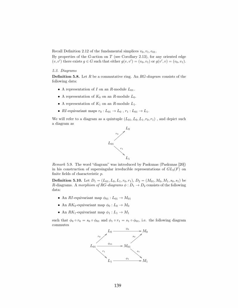
Recall Definition 2.12 of the fundamental simplices v0, v1, e01.By properties of the G-action on T (see Corollary 2.13), for any oriented edge(v, v′) there exists g ∈ G such that either g(v, v′) = (v0, v1) or g(v′, v) = (v0, v1).

5.3. DiagramsDefinition 5.8. Let R be a commutative ring. An RG-diagram consists of thefollowing data:

• A representation of I on an R-module L01.

• A representation of K0 on an R-module L0.

• A representation of K1 on an R-module L1.

• RI-equivariant maps r0 : L01 → L0 , r1 : L01 → L1.

We will refer to a diagram as a quintuple (L01, L0, L1, r0, r1) , and depict sucha diagram as

L0

L01

r0

==

r1

!!L1

Remark 5.9. The word “diagram” was introduced by Paskunas (Paskunas [20])in his construction of supersingular irreducible representations of GL2(F ) onfinite fields of characteristic p.

Definition 5.10. Let D1 = (L01, L0, L1, r0, r1), D2 = (M01,M0,M1, s0, s1) beR-diagrams. Amorphism of RG-diagrams φ : D1 → D2 consists of the followingdata:

• An RI-equivariant map φ01 : L01 →M01

• An RK0-equivariant map φ0 : L0 →M0

• An RK1-equivariant map φ1 : L1 →M1

such that φ0 ◦ r0 = s0 ◦ φ01 and φ1 ◦ r1 = s1 ◦ φ01, i.e. the following diagramcommutes

L0φ0 // M0

L01

r0

==

r1

!!

φ01 // M01

s0

<<

s1

""L1

φ1 // M1

139

The RG-diagrams with the above morphisms form a category, which we denoteby DiagRG.

5.4. Coefficient systems and induced representations

The coefficient systems on the tree will be intimately connected to certain rep-resentations of G. For this reason we introduce the following definition.

Proposition 5.11. There is an equivalence of categories between RG-diagramsand G-equivariant R-coefficient systems, that is DiagRG ' CoeffRG.

Proof. Consider the functor F : CoeffRG → DiagRG defined by

F (L) = (Le01, Lv0

, Lv1, re01v0, re01v1

), F (φ) = (φe01, φv0

, φv1)

for any G-equivariant R-coefficient system L = ({Lσ}σ⊂T , {rτσ}σ⊂τ ), and anyφ = {φσ}σ⊂τ ∈MorCoeffRG(L,M).Note that indeed, as K0,K1, I are the stabilizers of v0, v1, e01, respectively, sinceL is G-equivariant, we see that Le01

is an RI-module, Lv0is an RK0-module

and Lv1 is an RK1-module. In addition, it follows that the maps re01v0, re01v1

areRI-equivariant. It follows that F (L) ∈ Ob(DiagRG). Also, by definition of themorphisms we see that

φv0 ◦ re01v0

= se01v0◦ φe01 , φv1 ◦ re01

v1= se01

v1◦ φe01

so that F (φ) ∈MorDiagRG(L,M).Conversely, let D = (L01, L0, L1, r0, r1) be an RG-diagram. Let Vi = indGKi(Li)

and let V01 = indGI (L01).Since we have embeddings L0 ⊂ V0, L1 ⊂ V1 and L01 ⊂ V01, we think of the Li’sas embedded in the Vi’s, so that we have a G-action there, and we can considergLi.Recall that T0 = T 0

0

∐ T 10 and for any v ∈ T i0 , there exists g ∈ G such that

v = gvi. We set Lgvi = gLi ⊂ Vi. For any e ∈ T1, there exists g ∈ G such thate = ge01 and we set Lge01 = gL01 ⊂ V1.Note that this is well defined, since stabilizers of the vi act on Li, and thestabilizer of e01 acts on L01.Next, we desribe the G-action. If σ ⊂ T , either σ = ge01 or σ = gvi fori ∈ {0, 1}. Then either Lg′σ = Lg′ge01

= (g′g)Le01= g′Lσ or Lg′σ = Lg′gvi =

(g′g)Lvi = g′Lσ, so that the G-action is induced by its action on V0, V1 and V01,as G preserves types.Also, if σ ( τ , then τ ∈ T1 , and σ ∈ T0. In such a case, if σ ∈ T i0 , there existsg ∈ G such that τ = ge01 and σ = gvi.We set rτσ = rge01

gvi = grig−1, where the G-action is induced by its action on V01

and Vi. Again, this is well-defined, since ri are RI-equivariant, and I is thestabilizer of e01.

140

We claim that L = H(D) = ({Lσ}σ⊂T , {rτσ}σ⊂τ ) is aG-equivariant R-coefficientsystem.Indeed, since G acts on V0, V1, V01, we have (gh)σ = ghσ ·hσ for all g, h ∈ G andevery simplex σ ⊂ T , and 1σ = idLσ .Furthermore, by construction the rτσ satisfy rgτgσ ◦ gτ = gσ ◦ rτσ.Also, if φ : D1 → D2 is a morphism of diagrams, we set φgvi = gviφi

(g−1

)σif

σ = gvi ∈ T i0 and φσ = ge01φ01(g−1)σ if σ = ge01 ∈ T1.

We then let H(φ) = {φσ}σ⊂T , and as φgσ ◦ gσ = gσ ◦ φσ, andsge01gvi ◦ φge01

= sge01gvi ◦ ge01

◦ φ01 ◦ (g−1)ge01= gvi ◦ si ◦ φ01 ◦ (g−1)ge01

=

= gvi ◦ φi ◦ ri ◦ (g−1)ge01= φgvi ◦ gvi ◦ ri ◦ (g−1)ge01

= φgvi ◦ rge01gvi

we see that H(φ) ∈MorCoeffRG(H(D1), H(D2)).Clearly, F ◦H = idDiagRG , as F is simply a forgetful functor. Let us shows thatthere is a natural isomorphism η : H ◦ F → idCoeffRG .To avoid confusion, we will denote by L(g)σ the G-action on the G-equivariantR-coefficient system L. Consider the morphism ηL : (H ◦F )(L)→ L defined by

(ηL)gvi = L(g)vi ◦ ((H ◦ F )(L))(g−1)gvi

for i ∈ {0, 1, 01}. This is well defined, since for g ∈ Ki, both actions L(g) and(H ◦ F )(L)(g) coincide with the Ki-action on Li. (and I for L01, respectively).Moreover, this is an isomorphism, as we have an inverse given by

((H ◦ F )(L))(g)vi ◦ L(g−1)gvi

.Furthermore, for any g′ ∈ G we have

(ηL)g′gvi◦((H◦F )(L))(g′)gvi = L(g′g)vi◦((H◦F )(L))(g−1)gvi = L(g′)vi◦(ηL)gvi

and, denoting by (H ◦ F )(r) the restriction maps in (H ◦ F )(L) we also have

rge01gvi ◦ (ηL)ge01 = L(g)vi ◦ re01

vi ◦ ((H ◦F )(L))(g−1)ge01 = (ηL)gvi ◦ (H ◦F )(r)ge01gvi

showing that ηL is indeed a morphism of coefficient systems. Finally, we seethat the diagram

(H ◦ F )(L)ηL //

(H◦F )(φ)

��

Lφ

��(H ◦ F )(M)

ηM //Mcommutes for any φ : L →M. Indeed, for any σ = gvi ⊂ T we have

φσ ◦ (ηL)σ = φgvi ◦ L(g)vi ◦ ((H ◦ F )(L))(g−1)gvi =

=M(g)vi◦φvi◦((H◦F )(L))(g−1)gvi =M(g)vi◦(H◦F )(φ)vi◦((H◦F )(L))(g−1)gvi =

=M(g)vi ◦ ((H ◦ F )(M))(g−1)gvi ◦ (H ◦ F )(φ)gvi = (ηM)σ ◦ (H ◦ F )(φ)σ

showing that η is a natural isomorphism.

141

The above categorical equivalence in fact suggests the following interpretationof chains as induced representations.

Lemma 5.12. Let L be a G-equivariant R-coefficient system on T . Let L0 =L(v0), L1 = L(v1), and L01 = L(e01). Then

C0(L) ' indGK0L0 ⊕ indGK1

L1, C1(L) ' indGI L01

as RG-modules. Here indGHM denotes the compact induction of the R[H]-module M .

Proof. Let k ∈ {0, 1}. For any pointed k-simplex σ ⊂ Tk, and any k-chain ω ∈Ck(L), we let fσ,ω : G→ Lσ be the function defined by fσ,ω(g) = gg−1σω(g−1σ).Let K = stabG(σ) = {g ∈ G | gσ = σ}. Then for any k ∈ K

fσ,ω(kg) = (kg)g−1σω((kg)−1σ) = kσgg−1σω(g−1k−1σ) =

= kσ · gg−1σω(g−1σ) = k · fσ,ω(g)

Furthermore, ω has finite support, say S = supp(ω) ⊂ Tk. Let S ∩Gσ = {gασ |α ∈ A} be the elements of S in the orbit of σ under G, where gα ∈ G are someelements. Then A is finite.It follows that for g /∈ ⋃α∈AKg−1

α one has g−1 /∈ ⋃α∈A gαK, hence g−1σ /∈ S.Indeed, if g−1σ ∈ S, then there exists α ∈ A with g−1σ = gασ, hence g−1

α g−1σ =σ and g−1

α g−1 ∈ K so that g−1 ∈ gαK, contradiction.It follows that

fσ,ω(g) = gg−1σω(g−1σ) = gg−1σ(0) = 0

Therefore fσ,ω is finitely supported modulo K, hence fσ,ω ∈ indGKLσ.In addition, one has, under the G-action on indGKLσ, for any g, h ∈ G

(gfσ,ω)(h) = fσ,ω(hg) = (hg)(hg)−1σω((hg)−1σ) =

= hh−1σgg−1h−1σω(g−1h−1σ) = hh−1σ(gω)(h−1σ) = fσ,gω(h)

so that gfσ,ω = fσ,gω for any g ∈ G.Let us consider the maps ϕ0 : C0(L)→ indGK0

L0⊕ indGK1L1 and ψ0 : indGK0

L0⊕indGK1

L1 → C0(L), defined by

ϕ0(ω) = (fv0,ω, fv1,ω) , ψ0(f0, f1) = σ 7→{gv0(f0(g−1)) σ = gv0

gv1(f1(g−1)) σ = gv1

For any g ∈ G one has

ϕ0(gω) = (fv0,gω, fv1,gω) = (gfv0,ω, gfv1,ω) = g(fv0,ω, fv1,ω) = gϕ0(ω)

Therefore ϕ0 is G-equivariant.

142

Conversely, if f0 ∈ indGK0L0 and f1 ∈ indGK1

L1, then as they are compactlysupported modulo K0, K1, respectively, there exist finitely many elements inG, {gα}α∈A, {gβ}β∈B such that

supp(f0) ⊂⋃

α∈AK0gα, supp(f1) ⊂

⋃

β∈BK1gβ

Let S = {g−1α σ0 | α ∈ A} ∪ {g−1

β σ1 | β ∈ B}, and let σ ∈ T0 be such that σ /∈ S.If σ ∈ T 0

0 , then there exists g ∈ G such that σ = gv0. As σ /∈ S, we must havegv0 6= g−1

α v0 for any α ∈ A, so that g−1g−1α /∈ K0, hence g−1 /∈ K0gα for any

α ∈ A. It follows that g−1 /∈ ⋃α∈AK0gα, and in particular g−1 /∈ supp(f0).Thus

ψ0(f0, f1)(σ) = ψ0(f0, f1)(gv0) = gv0(f0(g−1)) = gv0

(0) = 0

Similarly, if σ ∈ T 10 , then σ = gv1 for some g ∈ G with g−1 /∈ ∪β∈BK1gβ , hence

g−1 /∈ supp(f1), so that

ψ0(f0, f1)(σ) = ψ0(f0, f1)(gv1) = gv1(f1(g−1)) = gv1(0) = 0

In any case, we see that supp(ψ0(f0, f1)) ⊂ S is finite. In addition, for anyσ ∈ T0, if σ ∈ T i0 for some i ∈ {0, 1}, let g ∈ G be such that σ = gvi, then

ψ0(f0, f1)(σ) = gvi(fi(g−1)) ∈ gviLi = Lgvi = Lσ

Therefore, we indeed see that ψ0(f0, f1) ∈ C0(L). In addition, for any g ∈ G,we see that for σ = hvi, i ∈ {0, 1} and h ∈ G one has

ψ0(g(f0, f1))(σ) = ψ0(gf0, gf1)(σ) = hvi((gfi)(h−1)) =

= hvi(fi(h−1g)) = gg−1hvi · (g−1h)vi(fi((g

−1h)−1)) =

= gg−1hvi · ψ0(f0, f1)(g−1hvi) = g(ψ0(f0, f1)(g−1σ)) = (g · ψ0(f0, f1))(σ)

Thus, ψ0(g(f0, f1)) = g · ψ0(f0, f1), showing that ψ0 is G-equivariant.Furthermore, for any ω ∈ C0(L) and any f0 ∈ indGK0

L0, f1 ∈ indGK1L1 we have

for any σ = gvi ∈ T i0 (here i ∈ {0, 1})

ψ0(ϕ0(ω))(σ) = gvi((ϕ0(ω))i(g−1)) = gvi(fvi,ω(g−1)) =

= gvi

((g−1

)gvi· ω(gvi)

)= ω(gvi) = ω(σ)

and for any g ∈ G

fvi,ψ0(f0,f1)(g) = gg−1viψ0(f0, f1)(g−1vi) = gg−1vi ·(g−1

)vi

(fi(g)) = fi(g)

Therefore fvi,ψ0(f0,f1) = fi and

ϕ0(ψ0(f0, f1)) = (fv0,ψ0(f0,f1), fv1,ψ0(f0,f1)) = (f0, f1)

143

This shows that ϕ0, ψ0 define isomorphisms of RG-modules

C0(L) ' indGK0L0 ⊕ indGK1

L1

Next, let us consider the maps ϕ1 : C1(L) → indGI (L01) and ψ1 : indGI L01 →C1(L), defined by

ϕ1(ω) = fe01,ω, ψ1(f) = σ 7→{ge01(f(g−1)) σ = ge01

−ge01(f(g−1)) σ = ge01

We have already shown that fe01,ω ∈ indGI (L01). Conversely, if f ∈ indGI L01, itis compactly supported modulo I, hence there exist finitely many elements inG, say {gα}α∈A such that supp(f) ⊂ ⋃α∈A Igα.Let S = {g−1

α e01}α∈A, and let σ ∈ T1 be such that σ, σ /∈ S. Since G actstransitively on the set of non-oriented edges T1, there exists g ∈ G such thateither σ = ge01 or σ = ge01.As σ, σ /∈ S, we must have ge01 6= g−1

α e01 for any α ∈ A, so that g−1g−1α /∈ I,

hence g−1 /∈ Igα, for any α ∈ A. In particular g−1 /∈ supp(f). Therefore

ψ1(f)(σ) =

{ψ1(f)(ge01) σ = ge01

ψ1(f)(ge01) σ = ge01

=

=

{ge01(f(g−1)) σ = ge01

−ge01(f(g−1)) σ = ge01

=

{ge01

(0) σ = ge01

−ge01(0) σ = ge01

= 0

It follows that supp(ψ1(f)) ⊂ S, hence ψ1 is finitely supported. In addition, forany σ ∈ T1, let g ∈ G be such that σ = ge01 or σ = ge01, then

ψ1(f)(σ) =

{ge01(f(g−1)) σ = ge01

−ge01(f(g−1)) σ = ge01

∈ ge01L01 = Lge01

= Lσ

Also, by definition ψ1(f)(σ) = −ψ1(f)(σ), hence ψ1(f) ∈ C1(L).For any g, h ∈ G one has

ϕ1(gω) = fe01,gω = g · fe01,ω = g · ϕ1(ω)

ψ1(g · f)(he01) = he01((gf)(h−1)) = he01

(f(h−1g)) =

= gg−1he01·(g−1h)e01

·f((g−1h)−1) = gg−1he01·ψ1(f)(g−1he01) = (g·ψ1(f))(he01)

showing that both ϕ1 and ψ1 are G-equivariant.Furthermore, for any ω ∈ C1(L) and any f ∈ indGI L01, we have for any σ =

ge01 ∈ T1 that

ψ1(ϕ1(ω))(σ) = ge01((ϕ1(ω))(g−1)) = ge01

(fe01,ω(g−1)) =

144

= ge01

((g−1

)ge01· ω(ge01)

)= ω(ge01) = ω(σ)

and for any g ∈ Gfe01,ψ1(f)(g) = gg−1e01

ψ1(f)(g−1e01) = gg−1e01·(g−1

)e01

(f(g)) = f(g)

Therefore fe01,ψ1(f) = f and

ϕ1(ψ1(f)) = fe01,ψ1(f) = f

This shows that ϕ1, ψ1 define isomorphisms of RG-modules

C1(L) ' indGI L01

Lemma 5.13. Let L be a G-equivariant R-coefficient system on T . Underthe isomorphisms in Lemma 5.12, the boundary map ∂ : C1(L) → C0(L) isdescribed as

∂([1, l01]) = ([1, r0(l01)], [1,−r1(l01)])

Here, we recall the definition of [g, v], as in (3.3).

Proof. Since indGI L01 consists of functions compactly supported mod H, andG acts by right translations, we see that it is spanned, as an RG-module byelements of the form [1, l]. Therefore, it suffices to describe ∂([1, l01]).However, using the morphism ψ1 in Lemma 5.12, we see that for any σ ∈ T1

ψ1([1, l01])(σ) =

{ge01([1, l01])(g−1) σ = ge01

−ge01([1, l01])(g−1) σ = ge01

=

=

ge01(g−1 · l01) σ = ge01, g ∈ I−ge01(g−1 · l01) σ = ge01, g ∈ I0 g /∈ I

=

l01 σ = e01

−l01 σ = e01

0 σ, σ 6= e01

So [1, l01] corresponds to the 1-chain supported on the single edge e01, hence∂(ψ1([1, l01])) is supported on the vertices v0, v1 and satisfies

∂(ψ1([1, l01]))(v0) = re01v0

(l01) = r0(l01)

∂(ψ1([1, l01]))(v1) = re01v1

(−l01) = −r1(l01)

Finally, we see that

∂([1, l01]) = ϕ0(∂(ψ1([1, l01]))) = ([1, r0(l01)], [1,−r1(l01)])

Corollary 5.14. The boundary map from the oriented 1-chains to the 0-chainsgives an exact sequence of RG-modules

0→ H1(L)→ indGI L01 → indGK0L0 ⊕ indGK1

L1 → H0(L)→ 0

145

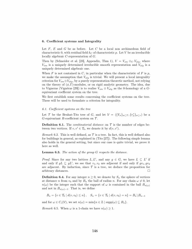
6. Coefficient systems and Integrality

Let F , E and G be as before. Let C be a local non archimedean field ofcharacteristic 0, with residual field kC of characteristic p. Let V be an irreduciblelocally algebraic C-representation of G.Then by (Schneider et al. [23], Appendix, Thm 1), V = Vsm ⊗C Valg, whereVsm is a uniquely determined irreducible smooth representation and Valg is auniquely determined algebraic one.When F is not contained in C, in particular when the characteristic of F is p,we make the assumption that Valg is trivial. We will present a local integralitycriterion for Vsm⊗Valg, by a purely representation theoretic method, not relyingon the theory of (φ,Γ)-modules, or on rigid analytic geometry. The idea, dueto Vigneras (Vignéras [29]) is to realise Vsm ⊗ Valg as the 0-homology of a G-equivariant coefficent system on the tree.We first establish some results concerning the coefficient systems on the tree.These will be used to formulate a criterion for integrality.

6.1. Coefficient systems on the tree

Let T be the Bruhat-Tits tree of G, and let V = ({Vσ}σ⊂T , {rτσ}σ⊂τ ) be aG-equivariant R-coefficient system on T .

Definition 6.1. The combinatorial distance on T is the number of edges be-tween two vertices. If v, v′ ∈ T0, we denote it by d(v, v′).

Remark 6.2. This is well defined, as T is a tree. In fact, this is well defined alsofor buildings in general, as explained in (Tits [27]). The following simple lemmaalso holds in the general setting, but since our case is quite trivial, we prove ithere as well.

Lemma 6.3. The action of the group G respects the distance.

Proof. Since for any two lattices L,L′, and any g ∈ G, we have L ⊆ L′ ifand only if gL ⊆ gL′, we see that v1, v2 are adjacent if and only if gv1, gv2

are adjacent. By induction, since T is a tree, we deduce the proposition forarbitrary distances.

Definition 6.4. For any integer n ≥ 0, we denote by Sn the sphere of verticesat distance n from v0 and by Bn the ball of radius n. For any chain ω 6= 0, letn(ω) be the integer such that the support of ω is contained in the ball Bn(ω)

and not in Bn(ω)−1. That is, we define

Bn = {v ∈ T0 | d(v, v0) ≤ n} , Sn = {v ∈ T0 | d(v, v0) = n} = Bn\Bn−1

and for ω ∈ Ci(V), we set n(ω) = min{n ∈ Z | supp(ω) ⊆ Bn}.

Remark 6.5. When ω is a 1-chain we have n(ω) ≥ 1.

146

Lemma 6.6. For any vertex v ∈ Sn with n ≥ 1, the neighbours of v belong toSn+1 except one neighbour which belongs to Sn−1.

Proof. Let w1, w2 ∈ Sn−1 be neighbours of v. Then by definition, there existpaths with no backtracking P1 = (v0, . . . , w1) and P2 = (v0, . . . , w2) of lengthn− 1.Furthermore, they do not intersect, since if P1 ∩ P2 6= ∅, take p = min{q ∈ P1 |q ∈ P1 ∩ P2} and obtain a cycle through v0 and p.It follows that P1vP

−12 = (v0, . . . , w1, v, w2, . . . , v0) is a cycle. But T is a tree,

hence it must contain backtracking, and as P1, P2 are non-intersecting paths,we must have (w1, v) = (w2, v), so that w1 = w2.

Notation 6.7. Let τv be the unique oriented edge starting from v and pointingtoward the origin v0.For any oriented 1-chain ω,

∂ω(v) = rτvv ω(τv) (6.1)

for all v ∈ Sn(ω).

For i = 0, 1, we identify naturally ui ∈ Vi = Vvi with a 0-chain supported onthe single vertex vi. We then consider the natural Ki-equivariant linear map

wi : Vi → H0(T ,V)

and the natural I-equivariant linear maps

w0 ◦ r0 : V01 → V0 → H0(T ,V), w1 ◦ r1 : V01 → V1 → H0(T ,V)

Lemma 6.8. If both r0, r1 are injective, then:1. the maps w0, w1 are injective.2. w0 ◦ r0 = w1 ◦ r1 is I-equivariant.

Proof. There is no non-zero 1-chain ω with ∂ω supported on the single vertexv0 because n(ω) ≥ 1 and ∂ω is not zero on Sn(ω) by (6.1) because r0, r1 areinjective. It follows that there is also no non-zero 1-chain ω with ∂ω supportedon the single vertex v1. As both wi and ri are I-equivariant, we have trivially theI-equivariance. Explicitly, if we consider ω, the oriented 1-chain with supporte01 such that ω(v0, v1) = u01 for some u01 ∈ V01, then we see that ∂ω is suchthat ∂ω(v0) = r0(u01) and ∂ω(v1) = −r1(u01), so that ∂ω = ω0−ω1, where ω1 isthe 0-chain with support v1 and value r1(u01) and ω0 is the 0-chain with supportv0 and value r0(u01). This shows that w1 ◦ r1 = w0 ◦ r0, as their difference is aboundary.

When ∂ is injective, we must have ker r0 ∩ ker r1 = 0. Indeed, else let u ∈ker r0 ∩ ker r1, and take ω to be the 1-chain supported on e01 with ω(e01) = u.By the formula (6.1) the converse is slightly weaker.

147

Lemma 6.9. ∂ is injective if both r0, r1 are injective.

Proof. Let ω 6= 0 be any oriented 1-chain and let v ∈ Sn(w); the edge τv belongsto the support of ω. By the formula (6.1), ∂ω(σ) = rτvv ω(τv) does not vanish.Indeed, as the G-action is transitive on each type, there exists g ∈ G such thatgv0 = v or gv1 = v and g(v0, v1) = τv (or −τv), whence either

0 = rτvv ω(τv) = rge01gv0◦ ge01

(g−1e01ω(τv)) = gv0

· re01v0

(g−1e01ω(τv)) = g · r0(g−1ω(τv))

or

0 = rτvv ω(τv) = rge01gv1◦ ge01(g−1

e01ω(τv)) = gv1 · re01

v1(g−1e01ω(τv)) = g · r1(g−1ω(τv))

But this implies (as the G-action is linear) that either r0(g−1ω(τv)) = 0 orr1(g−1ω(τv)) = 0, whence by injectivity of r0 and r1, g−1ω(τv) = 0, henceω(τv) = 0, contradiction.

We suppose from now on that the maps ri : V01 → Vi are injective.

Proposition 6.10. (Descent) Let φ 6= 0 be a 0-chain not supported only at theorigin. There exists an oriented 1-chain ω such that n(φ − ∂ω) < n(φ) if andonly if φ(v) ∈ rτvv Vτv for all v ∈ Sn(φ).

Proof. Let ω be an oriented 1-chain. By the formula (6.1), n(φ− ∂ω) < n(φ) isequivalent to n(ω) = n(φ) and

φ(v) = rτvv ω(τv)

for all v ∈ Sn(ω). When the necessary condition φ(v) ∈ rτvv Vτv is satisfied,say φ(v) = rτvv (vτv ) for some vτv ∈ Vτv for all v ∈ Sn(φ), the oriented 1-chainωφ supported on

⋃v∈Sn(φ)

τv with value vτv on τv, satisfies n(φ − ∂ω) < n(φ).The oriented 1-chains satisfying n(φ − ∂ω) < n(φ) are ωφ + ω′ where n(ω′) ≤n(φ)− 1.

When the R-module r0(V01) has a complement in V0, say V0 = W0⊕r0(V01), andv is of type 0, then the R-module rτvv (Vτv ) has a (non canonical) complement inVv, say Vv = Wv⊕rτv (Vτ ); Similarly, for v of type 1, when the R-module r1(V01)has a complement in V1, say V1 = W1 ⊕ r1(V01), and v is of type 1, then theR-module rτvv (Vτv ) has a (non canonical) complement in Vv.We can find an oriented 1-chain ω supported on τv such that (φ− ∂ω)(v) ∈Wv

for any v ∈ Sn(φ). By induction on n(φ), any nonzero element of H0(V) has arepresentative φ either supported at the origin, or such that φ(v) ∈Wv for anyv ∈ Sn(φ). (In fact, for all v).

148

6.2. Integrality local criterion

Let us first define what does it mean for a representation of G to be integral.

Proposition 6.11. Let R be a complete discrete valuation ring of fraction fieldS. An S-representation V of G of countable dimension is integral if it admitsa basis generating, over R, a G-stable R-submodule, L of V . L is called anR-integral structure.

We will now use the machinery of coefficient systems on the tree, as describedso far, to obtain a necessary and sufficient criterion for the integrality of therepresentation H0(V), for some coefficient systems V.

Definition 6.12. Let R be a complete DVR, and let S be its fraction field. LetL = ({Lσ}σ⊂T , {rτσ}σ⊂τ ) be a G-equivariant R-coefficient system, and letV :=L ⊗R S, rS,i := ri ⊗R idS : V01 → Vi for i ∈ {0, 1} be the corresponding G-equivariant S-coefficient system. Let i ∈ {0, 1}. We say that a chain ω ∈ Ci(V)is integral if ω ∈ Ci(L) ⊂ Ci(V).

By Lemma 6.8, the natural RK0-equivariant map w0 : L0 → H0(L) and thenatural RK1-equivariant map w1 : L1 → H0(L) are both injective, and thenatural map

w0 ◦ r0 = w1 ◦ r1 : L01 → H0(L)

is I-equivariant.We use this result to formulate and prove the following criterion, which is justa slight variation of the criterion due to Vigneras (Vignéras [29]), and the proofis essentially the same.

Proposition 6.13. 1) H1(L) = 0 if r0 and r1 are both injective. Conversely,if H1(L) = 0, then ker r0 ∩ ker r1 = 0.2) Integrality Local Criterion:Suppose that- R is a complete discrete valuation ring of fraction field S,- L0, L1 are free R-modules of finite rank,- r0, r1 are both injective,and let V := L ⊗R S, rS,i := ri ⊗R idS : V01 → Vi for i ∈ {0, 1}.Then, the map H0(L) → H0(V) is injective, hence the R-module H0(L) istorsion-free and contains no line S · h for h ∈ H0(V), when the equivalentconditions are satisfied:a) rS,0(V01) ∩ L0 = r0(L01) and rS,1(V01) ∩ L1 = r1(L01),b) the maps V01/L01 → V0/L0, V01/L01 → V1/L1 are both injective.c) r0(L01) is a direct factor of L0 and r1(L01) is a direct factor of L1, as R-modules.

149

Proof. of Proposition 6.131) By Lemma 6.9, ∂ : C1(L) → C0(L) is injective if ri : L01 → Li are bothinjective. However, H1(L) = ker ∂, hence we are done.2) As r0, r1 are injective, we can reduce them to inclusions L01 → L0, L01 → L1,and rS,0, rS,1 are inclusions V01 → V0, V01 → V1.Equivalence of the properties a), b), c):Note that V01 ∩ Li = L01 ⇐⇒ ker(V01 → Vi/Li) = L01 ⇐⇒ Li/L01 is torsion-free⇐⇒ L01 is a direct factor of Li (since Li is a free module of finite rank overthe PID R).We now turn to prove the conclusion:The R-module H0(L) embeds in the S-vector space H0(V) because the mapsV01/L01 → Vi/Li are injective by b) hence H1 (V/L) = 0 by 1) and the sequenceH1 (V/L)→ H0(L)→ H0(V) is exact.Let h be a nonzero element of H0(L). Suppose that the line Sh is containedin H0(L). We choose a generator, x, for the unique maximal ideal in R, andchoose- a representative φ ∈ C0(L) of h such that φ is supported on v0 or such thatφ(v) ∈Wv for any v ∈ Sn(φ)

- a vertex v′ ∈ Sn(φ) such that φ(v′) 6= 0.- an integer n ≥ 1 such that φ(v′) /∈ xnLv′ .Since S · h ⊂ H0(L), there exists an integral oriented 1-cocycle ω ∈ C1(L) suchthat (φ+ ∂ω)(v) ∈ xnLv for any vertex v ∈ T0.We may suppose n(ω) ≤ n(φ) by the following argument.If n(ω) > n(φ), the formula (6.1) implies that ω(τv) ∈ xnL(τv) for any vertexv ∈ Sn(ω) because rτvv Lτv ∩ xnLv = rτvv (xnLτv ) by a) and the injectivity of rτvv .Let ωext be the integral oriented 1-cocycle supported on

⋃v∈Sn(ω) τv and equal

to ω on this set. We may replace ω by ω − ωext; as n(ω − ωext) < n(ω) wereduce to n(ω) ≤ n(φ) by decreasing induction.If φ is supported on v0, then ω = 0 and φ(v0) ∈ xnL0 which is false.If nφ ≥ 1, we have φ(v)+ω(τv) ∈ xnLv for any v ∈ Sn(φ) by (6.1). As φ(v) ∈Wv

and ω(τv) ∈ rτvv (Vτv ), this is impossible.As R is a local complete PID, H0(L) is R-free.

Lemma 6.14. Let φ be a 0-chain supported at the single vertex v0 and let ω bean oriented 1-chain such that φ+ ∂ω is integral. Then φ is integral.

Proof. As n(ω) ≥ 1, the restriction of ω on Sn(ω) is integral by (6.1). By adecreasing induction on n(ω), φ is integral.

Corollary 6.15. When the properties of 2) (in Proposition 6.13) are true,H0(L) is an R-integral structure of H0(V) such that

H0(L) ∩ V0 = L0, H0(L) ∩ V1 = L1

150

The corollary in fact shows that the above criterion is sufficient for H0(V) tobe integral, where V = L ⊗R S. Next, we establish a necessary and sufficientcriterion.

Corollary 6.16. Let R be a complete discrete valuation ring of fraction fieldS, and let r0 : V01 → V0, r1 : V01 → V1 be the maps in the RG-diagramcorresponding to a G-equivariant R-coefficient system V. The S-representationH0(V) of G is R-integral if and only if there exist R-integral structures L0, L1

of the representations V0 of K0, V1 of K1, such that L01 = r−10 (L0) = r−1

1 (L1) .When this is true, the diagram

L0

L01

r0

==

r1

!!L1

defines a G-equivariant coefficient system L of R-modules on X , and H0(L) isan R-integral structure of H0(V).

Proof. of Corollary 6.16Sufficient. When L0, L1 are R-integral structures of V0, V1 such that L01 =r−10 (L0) = r−1

1 (L1), then L01 is an R-integral structure of V01; the maps r0, r1

induce an injective diagramL0

L01

==

!!L1

By the integrality criterion (Proposition 6.13), H0(V) is R-integral.Necessary. Suppose that L is an R-integral structure of H0(V). We applyLemma 6.8. The inverse image L0 of w0(V0) ∩ L in V0 by w0 is an R-integralstructure of the representation of K0 on V0, the inverse image L1 of w1(V1)∩Lin V1 by w1 is an R-integral structure of the representation of K1 on V1, andthe inverse image L01 of (w0 ◦ r0)(V01)∩L = (w1 ◦ r1)(V01)∩L is an R-integralstructure of V01, such that L01 = r−1

0 (L0) = r−11 (L1).

From now on, r0, r1 are injective and V0 = K0 · r0(V01), V1 = K1 · r1(V01).

Definition 6.17. When Vi, for i = 0, 1 identified with an element of Z/2Z,contains an R-integral structure Mi which is a finitely generated R-submodule,

151

one constructs inductively an increasing sequence of finitely generated R-integralstructures (zn(Mi))n≥1 of Vi, called the zigzags of Mi, as follows:The RKi+1-module Mi+1 defined by Mi+1 = Ki+1 · ri+1(r−1

i (Mi)) is an R-integral structure of the SKi+1-module Vi+1 (a finitely generated R-module isfree if and only if it is torsion free and does not contain an S-line). We repeatthis construction to get the first zigzag z(Mi):

z(Mi) = Ki · ri(r−1i+1

(Ki+1 · ri+1

(r−1i (Mi)

)))⊇Mi

Corollary 6.18. Let i ∈ Z/2Z and let Mi be an R-integral structure of theSKi-module Vi. The representation of G on H0(V) is R-integral if and only ifthe sequence of zigzags (zn(Mi))n≥0 is finite.

Proof. of Corollary 6.18When the sequence of zigzags is finite, there exists a finitely generated R-integralstructure Mi of Vi equal to its first zigzag z(Mi) = Mi, for i = 0 or i = 1. SetMi+1 = ri+1(r−1

i (Mi)). By definition of z(Mi), we see that

Mi = z(Mi) = Ki · ri(r−1i+1 (Ki+1 ·Mi+1)

)⊃ ri

(r−1i+1 (Ki+1 ·Mi+1)

)

henceMi+1 = ri+1

(r−1i (Mi)

)⊃ Ki+1 ·Mi+1

showing that Mi+1 ⊂ Vi+1 is Ki+1-stable, hence a finitely generated R-integralstructure of Vi+1, such that r−1

i+1(Mi+1) = r−1i (Mi).

Conversely, let Mi be an R-integral structure of Vi. Replacing L by a multiple,we suppose Mi ⊂ Li. Then r−1

i (Mi) ⊂ r−1i (Li) = r−1

i+1(Li+1), hence Ki+1 ·ri+1

(r−1i (Mi)

)⊂ Li+1 and z(Mi) ⊂ Li. The sequence of zigzags of Mi is

contained in Li and increasing, hence finite because Li is a finitely generatedR-module and R is noetherian.

6.3. Integrality criterion for locally algebraic representations

The main idea allowing us to make use of the above criterion for arbitraryirreducible locally algebraic representations, is the fact that any such represen-tation can be obtained as the 0-homology of some coefficient system on the tree.This was shown for smooth representations over C by Schneider and Stuhler inSchneider and Stuhler [21], and we will extend the result further here. Theproof is the same as in Vignéras [29] for the case G = GL2(F ).In order to formulate the results, we will use the filtrations previously describedof the stabilizers (see subsection 2.3).

Lemma 6.19. We have group homomorphisms:When E/F is unramified

K0/K0(1) ' U3(kF ), K1/K1(1) ' H(kF ), I/I(1) 'M(kF )

152

while for E/F ramified we have

K0/K0(1) ' O3(kF ), K1/K1(1) ' H′(kF ), I/I(1) 'M′(kF )

and further bijections, when E/F is unramified

B ∩K0\K0/K0(1) ' B(kF )\G(kF )

B ∩K1\K1/K1(1) 'M(kF )Z(kF )\H(kF )

and when E/F is ramified

B ∩K0\K0/K0(1) ' B′(kF )\O3(kF )

B ∩K1\K1/K1(1) 'M′(kF )Z′(kF )\H′(kF )

Here G(kF ) = U3(kF ) = {g ∈ GL3(kE) |t gθg = θ} is the unitary groupin three variables, O3(kF ) = {g ∈ GL3(kF ) |t gθg = θ} is the correspondingorthogonal group in three variables, B(kF ),B′(kF ) are the Borel subgroups ofupper triangular matrices in U3(kF ),O3(kF ), respectively, M(kF ),M′(kF ) thecorresponding Levi qoutients, and

H(kF ) =

a 0 b0 c 0d 0 e

| c ∈ k1

E , ad, be ∈ k−E , ae+ db = 1

≤ G(kF )

H′(kF ) =

a 0 b0 ±1 0c 0 d

| ad− bc = 1

≤ O3(kF )

Z(kF ) =

1 0 z0 1 00 0 1

| z ∈ kE , z + z = 0

Z′(kF ) =

1 0 z0 1 00 0 1

| z ∈ kF

Proof. We have natural maps K0 → U3(kF ), I → M(kF ) in the unramifiedcase, and K0 → O3(kF ), I → M′(kF ) in the ramified case, by reducing eachentry mod πOE , and zeroes above the main diagonal in the latter map. Furtherwe have a map ρ : K1 → H(kF ) in the unramified case, or ρ : K1 → H′(kF ) inthe ramified case defined by

ρ

a b π−1cπd e fπg πh i

=

a mod π 0 c mod π0 e mod π 0

g mod π 0 i mod π

Note that K0(1), I(1) and K1(1) are precisely the kernels of these surjectivemaps to obtain the required result.

153

For the bijections, note that B ∩ K0 is the preimage of B(kF ), B′(kF ) underthe reduction maps K0 → G(kF ), K0 → O3(kF ), while B ∩K1 is the preimageof M(kF )Z(kF ), M′(kF )Z′(kF ) under the reduction maps K1 → H(kF ), K1 →H′(kF ).

Proposition 6.20. Let Valg be an irreducible algebraic C-representation ofG (hence E ⊂ C if Valg is not trivial), let Vsm be a finite length smooth C-representation of G and let e be an integer ≥ 1 such that Vsm is generated byits K0(e)-invariants.1) The locally algebraic C-representation V := Vsm ⊗C Valg of G is isomor-phic to the 0-th homology H0(V) of the coefficient system V associated with theinclusions

VK0(e)sm ⊗C Valg

VI(e)sm ⊗C Valg

77

((VK1(e)sm ⊗C Valg

2) The representation of G on V is OC-integral if and only if there exist OC-integral structures L0, L1 of the representations of K0,K1 on V

K0(e)sm ⊗C Valg,

VK1(e)sm ⊗CValg respectively such that L01 := L0∩(V

I(e)sm ⊗CValg) = L1∩(V

I(e)sm ⊗C

Valg). Then the 0-th homology L of the G-equivariant coefficient system on Xdefined by the diagram

L0

L01

==

!!L1

is an OC-structure of V .

Proof. of Proposition 6.201) The exactness of the sequence

0→ indGI

(V I(e)sm ⊗C Valg

)→ indGK0

(V K0(e)sm ⊗C Valg

)⊕indGK1

(V K1(e)sm ⊗C Valg

)→

→ Vsm ⊗C Valg → 0

follows from the following facts.The assertion is true when Valg is trivial if C is replaced by the field C of complexnumbers by (Schneider and Stuhler [21] II.3.1); This is also true for C because

154

the scalar extension ⊗CC commutes with the invariants by an open compactsubgroup and with the compact induction from an open subgroup. The tensorproduct by ⊗CValg of an exact sequence of CG-representations remains exactand commutes with the compact induction from an open subgroup.2) The finite length representation Vsm is admissible; this is known for complexrepresentations and remains true for C-representations because Vsm ⊗C C hasfinite length (Vignéras [28] II.43.c), and · ⊗C C commutes with the Ki(e)-invariant functor. The C-vector spaces V Ki(e)sm ⊗C Valg are finite dimensional.Apply Corollary 6.16.

We have L0 = L∩(VK0(e)sm ⊗Valg) and L1 = L∩

(VK1(e)sm ⊗ Valg

)in 2) by Lemma

6.14; when (VK0(e)sm ⊗C Valg) = K0 · (V I(e)sm ⊗C Valg) and (V

K1(e)sm ⊗C Valg) =

K1 · (V I(e)sm ⊗C Valg), one can suppose L0 = K0L01 and L1 = K1L01 in 2) byCorollary 6.18.We define the contragredient V = Vsm⊗C V

′alg of V = Vsm⊗C Valg by tensoring

the smooth contragredient Vsm of Vsm and the linear contragredient V′alg of Valg.

Corollary 6.21. A finite length locally algebraic C-representation of G is OC-integral if and only if its contragredient is OC-integral.

Proof. of Corollary 6.21Let Vsm be a nonzero smooth C-representation of G of finite length; thereexists an integer e ≥ 1 such that each nonzero irreducible subquotient of Vsmcontains a nonzero Ki(e)-invariant vector, by smoothness. The C-vector space(Vsm

)Ki(e)is isomorphic to the dual

(VKi(e)sm

)′; the irreducible subquotients of

the contragredient Vsm are the contragredients of the irreducible subquotientsof Vsm. Hence Vsm and Vsm are generated by their K0(e)-invariants.Suppose that V = Vsm ⊗C Valg is OC-integral. We choose OC-integral struc-tures L0 of the representation of K0 on V

K0(e)sm ⊗C Valg and L1 of the repre-

sentation of K1 on VK1(e)sm ⊗C Valg such that L01 := L1 ∩

(VI(e)sm ⊗C Valg

)=

L0 ∩(VI(e)sm ⊗C Valg

)(Proposition 6.20), and we take the linear duals L

′0 =

HomOC (L0,OC) of L0 and L′1 = HomOC (L1,OC) of L1. It is clear that L

′i is

an OC-integral structure of the representation of Ki on

(V Ki(e)sm ⊗C Valg

)′'(V Ki(e)sm

)′⊗C (Valg)

′'(Vsm

)Ki(e)⊗C V

′alg

We take the intersection L′i ∩((

Vsm

)I(e)⊗C V

′alg

)= L

′i ∩(VI(e)sm ⊗C Valg

)′.

The OC-module L01 is a direct factor of L0 and L1, hence its linear dual L′01 is

equal to this intersection. By Proposition 6.20, V is OC-integral.

155

From now on, we assume Valg = C, i.e. the algebraic part is trivial, and therepresentation is smooth.We conclude this part by considering inflations of diagrams.

Definition 6.22. A tamely ramified diagram is a diagramD = (L01, L0, L1, r0, r1)such that

• K0(1) acts trivially on L0.

• K1(1) acts trivially on L1.

• I(1) acts trivially on L01, and it is semi-simple as an SI-module.

• r0, r1 are injective.

Lemma 6.23. A tamely ramified diagram is equivalent (by “inflation”) to thefollowing data if E/F is unramified:

• an R-representation Y0 of U3(kF ).

• an R-representation Y1 of H(kF ).

• a semi-simple R-representation Y01 of M(kF ).

• RM(kF )-inculsions Y01 → Y0 and Y01 → Y1 with images contained inY

N(kF )0 and Y Z(kF )

1 respectively.

and to to the following data if E/F is ramified:

• an R-representation Y0 of O3(kF ).

• an R-representation Y1 of H′(kF ).

• a semi-simple R-representation Y01 of M′(kF ).

• RM′(kF )-inculsions Y01 → Y0 and Y01 → Y1 with images contained inY

N′(kF )0 and Y Z′(kF )

1 respectively.

The action of K0 on L0 inflates the action of Y0, the action of K1 on L1 inflatesthe action of Y1, the action of I on L01 inflates the action of Y01.Here,

N′(kF ) =

nb,z =

1 b z0 1 −b0 0 1

| 2b+ z2 = 0, b, z ∈ kF

≤ O3(kF )

is its unipotent radical. If p 6= 2, z = −b2/2, and we denote nb = nb,z. If p = 2,then b = 0.

Proof. This is an immediate consequence of Lemma 6.19.

156

7. Integrality of principal series representations

We will make explicit the integral structures contsructed in Proposition 6.20,when V = Vsm is a smooth tamely ramified principal series representation.When χ⊗χ1 is tamely ramified, i.e. trivial on M ∩ I(1), its restriction to M ∩ Iis the inflation of a C-character η ⊗ η1 of M(kF ), and the principal series isthe 0-th homology of the G-equivariant coefficient system defined by the tamelyramified diagram

(indGB(χ⊗ χ1)

)K0(1)

(indGB(χ⊗ χ1)

)I(1)

55

))(indGB(χ⊗ χ1)

)K1(1)

inflated, in the case of E/F unramified, from the inclusions (see Lemma 7.2)

(ind

G(kF )B(kF ) (η ⊗ η1)

)N(kF )

→ indG(kF )B(kF ) (η ⊗ η1)

(ind

H(kF )M(kF )Z(kF )(η ⊗ η1)

)Z(kF )

→ indH(kF )M(kF )Z(kF )(η ⊗ η1)

and in the case of E/F ramified, from the inclusions (see Lemma 7.2)

(ind

O3(kF )B′(kF ) (η ⊗ η1)

)N′(kF )

→ indO3(kF )B′(kF ) (η ⊗ η1)

(ind

H′(kF )M′(kF )Z′(kF )(η ⊗ η1)

)Z′(kF )

→ indH′(kF )M′(kF )Z′(kF )(η ⊗ η1)

Note that(ind

G(kF )B(kF ) (η ⊗ η1)

)N(kF )

= C ·φ1⊕C ·φs , where φ1, φs have supportsB(kF ), B(kF )sN(kF ) and value 1 at id, s, respectively. Clearly,

Y01 := OC · φ1 ⊕OC · φs

is an OC-integral structure of(ind

G(kF )B(kF ) (η ⊗ η1)

)N(kF )

and

Y1 := H(kF ) · Y01, Y0 := G(kF ) · Y Z(kF )1

are OC-integral structures of indH(kF )M(kF )Z(kF )(η ⊗ η1) and indG(kF )

B(kF ) (η ⊗ η1).

157

Similarly, note that(ind

O3(kF )B′(kF ) (η ⊗ η1)

)N′(kF )

= C · φ1 ⊕ C · φs , where φ1, φs

have supports B′(kF ), B′(kF )sN′(kF ) and value 1 at id, s, respectively. Clearly,

Y01 := OC · φ1 ⊕OC · φs

is an OC-integral structure of(ind

O3(kF )B′(kF ) (η ⊗ η1)

)N′(kF )

and

Y1 := H′(kF ) · Y01, Y0 := O3(kF ) · Y Z′(kF )01

are OC-integral structures of indH′(kF )

M′(kF )Z′(kF )(η ⊗ η1) and indG′(kF )

B′(kF ) (η ⊗ η1).

Now (Y0, Y1, Y01) inflates to a tamely ramified diagram

LY0= K0 · LY01

LY01

88

''LY1 = K1 · LY1

defining a G-equivariant coefficient system L of free OC-modules of finite rankon T .

7.1. Integrality criterion for smooth principal series representations

In this section we will prove the following theorem -

Theorem 7.1. Suppose that the character χ⊗ χ1 is tamely ramified, and thatC contains a p-th root of 1. The following properties are equivalent:a) the principal series representation indGB(χ⊗ χ1) is OC-integral.b) χ−1(π), χ(π)q2 are integral.

c) Y N(kF )0 = Y01 = Y

Z(kF )1 , when E/F is unramified, while Y N′(kF )

0 = Y01 =

YZ′(kF )1 when E/F is ramified.

d) L := H0(L) is an OC-integral structure of indGB(χ⊗ χ1).When they are satisfied, we have LK0(1) = LY0

, LK1(1) = LY1and LI(1) = LY01

generates the OCG-module L.

Note that we may reduce to the case χ1 = 1, twisting by a central character.Hence, it suffices to assume χ tamely ramified and χ1 = 1.As χ is a tamely ramified character, η = χ �O×E is the inflation of a character ofF×q = k×E ' O

×E/(1+πOE), that we denote by the same letter, η.

We will also denote χ(π) = λ, so that χ(x) = λvE(x) · η(xπ−vE(x)), where vE isthe standard valuation on E (normalized such that vE(π) = 1).

158

Lemma 7.2. Let χ : E× → C be a tamely ramified character. It induces acharacter η : F×q → C. We have, when E/F is unramified,

(indGBχ

)K0(1) ∼= indU3(kF )B(kF ) η,

(indGBχ

)K1(1) ∼= indH(kF )M(kF )Z(kF )η

and when E/F is ramified,

(indGBχ

)K0(1) ∼= indO3(kF )B′(kF ) η,

(indGBχ

)K1(1) ∼= indH′(kF )M′(kF )Z′(kF )η

Proof. As G = BK0 = BK1, by the Iwasawa decompositon (Lemma 2.17), wesee that (

indGBχ)�K0' indK0

B∩K0η,

(indGBχ

)�K1' indK1

B∩K1η

and the representations of K0,K1 on(indGBχ

)K0(1),(indGBχ

)K1(1) , respectively,are the inflations of the principal series representations (see Lemma 6.23)

indG(kF )B(kF )η, ind

H(kF )M(kF )Z(kF )η

when E/F is unramified, and inflations of the principal series representations

indO3(kF )B′(kF ) η, ind

H′(kF )M′(kF )Z′(kF )η

when E/F is ramified.

In what follows we will introduce the set-up for our proof.

We construct explicit integral structures in V0 = (indGBχ)K0(1), V1 =(indGBχ

)K1(1),

and compute their preimages in V01 =(indGBχ

)I(1).We will begin our zig-zag by considering the natural choice of an integral struc-ture in V0 =

(indGBχ

)K0(1).

7.1.1. The integral structure L0

Let L0 be the OC-integral structure of the C-representation of K0 on V0 =(indK0

B∩K0η)K0(1)

given by the functions with values in OC .We denote by fg ∈ L0 the function of support (B ∩K0) gK0(1) and value 1 atg.When E/F is unramified, a system of representatives for B ∩K0\K0/K0(1) 'B(kF )\G(kF ) (see Lemma 6.19) is

1, sn for n ∈ N(kF ), s =

0 0 10 1 01 0 0

as follows from the Bruhat decomposition G(kF ) = B(kF )∐

B(kF )sN(kF ).

159

When E/F is ramified, a system of representatives for B ∩ K0\K0/K0(1) 'B′(kF )\O3(kF ) (see Lemma 6.19) is

1, sn for n ∈ N′(kF )

as follows from the Bruhat decomposition O3(kF ) = B′(kF )∐

B′(kF )sN′(kF ).

Therefore, an OC-basis of L0 is{f1, (fsn)n∈N(kF )

}when E/F is unramified,

and{f1, (fsn)n∈N′(kF )

}when E/F is ramified. Note that for any nb,z ∈ N(kF )

we have

n−1b,z =

1 b z

0 1 −b0 0 1

−1

=

1 −b z

0 1 b0 0 1

= n−b,z

Similarly, in the ramified case, n−1b = n−b and when p = 2, n−1

z = nz.In what follows, if E/F is unramified, we will denote by ρ0 : K0 → G(kF ) andρ1 : K1 → H(kF ) the two natural reductions, while if E/F is ramified, we willuse the same notations, only that ρ0 : K0 → O3(kF ) and ρ1 : K1 → H′(kF ).The following property of L0 will turn useful when computing its zig-zag.

Proposition 7.3. The OCK0-module L0 is cyclic, generated by f1, i.e. L0 =OCK0 · f1.

Proof. For all n ∈ N(kF ), and all g ∈ K0, one has

nsf1(g) = f1(gns) =

{χ(gns) ρ0(gns) ∈ B(kF )

0 else=

=

{χ(gns) ρ0(g) ∈ B(kF )ρ0(sn−1)

0 else= fsn−1(g)

so thatnsf1 = fsn−1

for all n ∈ N(kF ). In particular, fsn = n−1s · f1 ∈ OCK0 · f1 for any basiselement, establishing the proposition when E/F is unramified.When E/F is ramified, we obtain similarly that fsn = n−1s · f1 ∈ OCK0 · f1 forany n ∈ N′(kF ), finishing the proof.

We next describe the intersection of L0 with V01 =(indGBχ

)I(1)= V

I(1)0 .

Lemma 7.4. A system of representatives for I(1)/K0(1) is N(kF ) when E/Fis unramified, or by N′(kF ) when E/F is ramified. Thus, a basis of LI(1)

0 isgiven by

f1,∑

n∈N(kF )

fsn

160

in the former case, and byf1,

∑

n∈N′(kF )

fsn

in the latter.

Proof. Consider the natural reduction map ρ : K0 → U3(kF ), when E/F isunramified, and ρ : K0 → O3(kF ) when E/F is ramified.Then K0(1) = ker ρ, showing that I(1)/K0(1) ' ρ(I(1)). However, I(1) =ρ−1(N(kF )) when E/F is unramified, while I(1) = ρ−1(N′(kF )) when E/F isramified.This establishes the first claim.It follows that in both cases

B · I(1) =⋃

n

BnK0(1) = BK0(1)

andBsI(1) =

⋃

n

BsnK0(1) =∐

n

BsnK0(1)

Let φ1, φs ∈ V01 =(indGBχ

)I(1) be the functions with supports B · I(1) =B ·K0(1), BsI(1) and value 1 at 1, s respectively.As I(1) =

∐n nK0(1), and φs(sn) = φs(s) = 1, we see that r0 with respect to

the above bases isr0(φ1) = f1, r0(φs) =

∑

n

fsn (7.1)

and the result follows.

We also have a corresponding integral structure in V1 =(indGBχ

)K1(1), whichwe now introduce.

7.1.2. The integral structure L1

Let L1 be the OC-integral structure of the C-representation of K1 on V1 =(indK1

B∩K1η)K1(1)

given by the functions with values in OC .We denote by hg ∈ L1 the function of support (B ∩K1) gK1(1) and value 1 atg.When E/F is unramified, a system of representatives of B ∩K1\K1/K1(1) 'M(kF )Z(kF )\H(kF ) (see Lemma 6.19) is

1, tz for z ∈ Z(kF ), t =

0 0 π−1

0 1 0π 0 0

by the Bruhat decomposition H(kF ) = M(kF )Z(kF )∐

M(kF )Z(kF )sZ(kF ).

161

When E/F is ramified, a system of representatives of B ∩ K1\K1/K1(1) 'M′(kF )Z′(kF )\H′(kF ) (see Lemma 6.19) is

{1, tz}z∈Z′(kF )

Therefore, an OC-basis of L1 is {h1, htz}z∈Z(kF ) if E/F is unramified, and{h1, htz}z∈Z′(kF ) if E/F is ramified.

Proposition 7.5. The OCK1-module L1 is cyclic, generated by ht, i.e. L1 =OCK1 · ht.

Proof. For any z ∈ F−q and any g ∈ K1, one has

n0,π−1zth1(g) = h1(gn0,π−1zt) =

{χ(gn0,π−1zt) ρ1(gn0,π−1zt) ∈M(kF )Z(kF )

0 else=

=

{χ(gn0,π−1zt) ρ1(g) ∈M(kF )Z(kF )ρ1(tn0,π−1z)

0 else= htn0,π−1z

(g)

since M(kF )Z(kF )ρ1(tn0,π−1z) = M(kF )Z(kF )ρ1(tn0,π−1z). Thus

n0,π−1zth1 = htn0,π−1z

for z ∈ F−q . In particular, for all z ∈ F−q , one has htn0,π−1z= n0,π−1zth1 ∈

OCK1 · h1, showing the proposition when E/F is unramified.Similarly, for any z ∈ Fq and any g ∈ K1, one has

n0,π−1zth1(g) = h1(gn0,π−1zt) =

{χ(gn0,π−1zt) ρ1(gn0,π−1zt) ∈M′(kF )Z′(kF )

0 else=

=

{χ(gn0,π−1zt) ρ1(g) ∈M′(kF )Z′(kF )ρ1(tn−1

0,π−1z)

0 else= htn0,−π−1z

(g)

since M′(kF )Z′(kF )ρ1(tn−10,π−1z) = M′(kF )Z′(kF )ρ1(tn0,π−1z). Thus

n0,π−1zth1 = htn0,−π−1z

But ht = th1, hence h1 = tht, thus establishing the proposition.

Lemma 7.6. A system of representatives for I(1)/K1(1) is (sn0,πzs)z∈F−q whenE/F is unramified, and (sn0,πzs)z∈Fq when E/F is ramified. Thus, when E/Fis unramified

r1(φ1) = h1 +∑

y∈F−q

η?(y) · htn0,π−1y, r1(φs) = λ−1 · ht

and when E/F is ramified,

r1(φ1) = h1 +∑

y∈Fqη−1(y) · htn0,π−1y

, r1(φs) = λ−1 · ht

162

Proof. Note that when E/F is unramified, one has

I(1)/K1(1) ' K1/I(1)\K1/K1(1) 'M(kF )Z(kF )\H(kF )

so by the Bruhat decomposition H(kF ) = Z−(kF )M(kF )Z(kF ), we see that(sn0,πzs)z∈F−q is indeed a system of representatives for I(1)/K1(1).

When E/F is ramified, one has

I(1)/K1(1) ∼= K1/I(1)\K1/K1(1) ∼= M′(kF )Z′(kF )\H′(kF )

so by the Bruhat decomposition H′(kF ) = Z′−(kF )M′(kF )Z′(kF ), we see that

(sn0,πzs)z∈Fq is indeed a system of representatives for I(1)/K1(1).Further, we have for any 0 6= z ∈ Fq, that

sn0,πzs =

1 0 00 1 0πz 0 1

=

−z−1 0 π−1

0 1 00 0 z

0 0 π−1

0 1 0π 0 z−1

=

=

−z−1 0 π−1

0 1 00 0 z

0 0 π−1

0 1 0π 0 0

1 0 π−1z−1

0 1 00 0 1

∈ Btn0,π−1z−1

It follows that when E/F is unramified, one has

B · I(1) =⋃

z∈F−q

Bsn0,πzsK1(1) = PK1(1) ∪

⋃

06=z∈F−q

Btn0,π−1zK1(1)

and

BsI(1) = BsK1(1) ∪

⋃

06=z∈F−q

Bn0,πzsK1(1)

= BsK1(1)

while if E/F is ramified, one has

B · I(1) =⋃

z∈FqBsn0,πzsK1(1) = BK1(1) ∪

⋃

0 6=z∈FqBtn0,π−1zK1(1)

and

BsI(1) = BsK1(1) ∪

⋃

06=z∈FqBn0,πzsK1(1)

= BsK1(1)

Moreover

φ1(tn0,π−1z) = φ1

z−1 0 π−1

0 1 00 0 z

·

1 0 00 1 0

πz−1 0 1

=

163

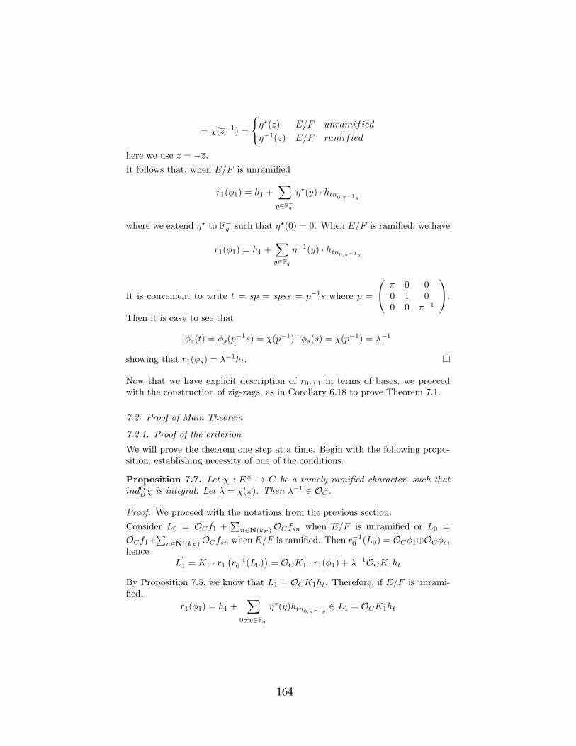
= χ(z−1) =

{η?(z) E/F unramified

η−1(z) E/F ramified

here we use z = −z.It follows that, when E/F is unramified

r1(φ1) = h1 +∑

y∈F−q

η?(y) · htn0,π−1y

where we extend η? to F−q such that η?(0) = 0. When E/F is ramified, we have

r1(φ1) = h1 +∑

y∈Fqη−1(y) · htn0,π−1y

It is convenient to write t = sp = spss = p−1s where p =

π 0 00 1 00 0 π−1

.

Then it is easy to see that

φs(t) = φs(p−1s) = χ(p−1) · φs(s) = χ(p−1) = λ−1

showing that r1(φs) = λ−1ht.

Now that we have explicit description of r0, r1 in terms of bases, we proceedwith the construction of zig-zags, as in Corollary 6.18 to prove Theorem 7.1.

7.2. Proof of Main Theorem

7.2.1. Proof of the criterion

We will prove the theorem one step at a time. Begin with the following propo-sition, establishing necessity of one of the conditions.

Proposition 7.7. Let χ : E× → C be a tamely ramified character, such thatindGBχ is integral. Let λ = χ(π). Then λ−1 ∈ OC .

Proof. We proceed with the notations from the previous section.Consider L0 = OCf1 +

∑n∈N(kF )OCfsn when E/F is unramified or L0 =

OCf1+∑n∈N′(kF )OCfsn when E/F is ramified. Then r−1

0 (L0) = OCφ1⊕OCφs,hence

L′1 = K1 · r1

(r−10 (L0)

)= OCK1 · r1(φ1) + λ−1OCK1ht

By Proposition 7.5, we know that L1 = OCK1ht. Therefore, if E/F is unrami-fied,

r1(φ1) = h1 +∑

06=y∈F−q

η?(y)htn0,π−1y∈ L1 = OCK1ht

164

while if E/F is ramified

r1(φ1) = h1 +∑

06=y∈Fqη−1(y)htn0,π−1y

∈ L1 = OCK1ht

and it follows that λ−1r1(φ1) ∈ L′1, so that λ−1f1 ∈ r0(r−11 (L1)) ⊂ z(L0).

But L0 = OCK0f1, hence λ−1L0 ⊂ z(L0). If the sequence of zigzags (zn(L0))n≥0

is finite, then we must have λ−1 ∈ OC .By Corollary 6.18, if λ−1 /∈ OC then indGBχ is not integral.

This also yields the easiest case for sufficiency, namely

Corollary 7.8. If λ ∈ O×C , then indGBχ is integral.

Proof. Consider the description of L′1 given above. If λ ∈ O×C , it follows that

λ−1OCK1ht = OCK1ht = L1.Since r1(φ1) ∈ L1, it follows that L

′1 = L1. Thus we see that r−1

0 (L0) = r−11 (L1),

and by Corollary 6.16, we see that indGBχ is integral.

Next, we turn to compute an explicit basis for L′1.

Lemma 7.9. For any z ∈ F−q when E/F is unramified, and for any z ∈ Fqwhen E/F is ramified, denote

Hz = tn0,π−1z · r1(φ1) ∈ L′1

Then L′1 is spanned over OC by

{Hz}z∈F−q , r1(φ1),{λ−1htn0,π−1z

}z∈F−q

, λ−1h1

when E/F is unramified, and by

{Hz}z∈Fq , r1(φ1),{λ−1htn0,π−1z

}z∈Fq

, λ−1h1

when E/F is ramified.

Proof. Note that using Lemma 6.19, one has

K1/I ' K1/K1(1)/I/K1(1) '{

H(kF )/M(kF )Z−(kF ) E/F unramifiedH′(kF )/M′(kF )Z

′−(kF ) E/F ramified

where Z−(kF ) = sZ(kF )s and Z′−(kF ) = sZ′(kF )s. Hence, by the Bruhat

decomoposition, a system of representatives for K1/I is

{1, tn0,π−1z | z ∈ F−q } if E/F is unramified

165

{1, tn0,π−1z | z ∈ Fq} if E/F is ramified

Note that as r−10 (L0) is I-invariant, and r1 is I-equivariant, it is enough to con-

sider the action of these representatives in order to obtain an explicit descriptionof L

′1. That is

L′1 = OCr1(φ1) +

∑

z∈F−q

OCtn0,π−1zr1(φ1) + λ−1L1

when E/F is unramified, and

L′1 = OCr1(φ1) +

∑

z∈FqOCtn0,π−1zr1(φ1) + λ−1L1

when E/F is ramified, but this is just the required result.

Lemma 7.10. Recall that we have defined Corollary 6.18, z(L0) = K0·r0(r−1(L1)).We now have, when E/F is unramified

q1/2λ · r0(φs) ∈ z(L0)


qλ · r0(φs) ∈ z(L0)

Proof. We first note that when E/F is unramified

Hz = tn0,π−1z ·

h1 +

∑

06=y∈F−q

η?(y)htn0,π−1y

=

= ht + η?(z)h1 +∑

0,z 6=y∈F−q

η?(y) · η(y − z) · htn0,π−1(y−z)−1 =

= η?(z)h1 + ht +∑

0,−z−1 6=y∈F−q

η?(y−1 + z) · η?(y) · htn0,π−1y=

= ht + η?(z)h1 +∑

06=y∈F−q

η?(1 + yz) · htn0,π−1y

If E/F is ramified, we see that

Hz = tn0,π−1z ·

h1 +

∑

06=y∈Fqη−1(y)htn0,π−1y

=

= ht + η−1(z)h1 +∑

0,z 6=y∈Fqη−1(y) · η(y − z) · htn0,π−1(y−z)−1 =

166

= η−1(z)h1 + ht +∑

0,−z−1 6=y∈Fqη−1(y−1 + z) · η−1(y) · htn0,π−1y

=

= ht + η−1(z)h1 +∑

06=y∈Fqη−1(1 + yz) · htn0,π−1y

When E/F is unramified, consider the sum∑

z∈F−q

Hz = q1/2ht +∑

z∈F−q

η?(z) · h1 +∑

06=y∈F−q

∑

z∈F−q

η?(1 + yz) · htn0,π−1y

and when E/F is ramified, consider the sum∑

z∈FqHz = qht +

∑

z∈Fqη−1(z) · h1 +

∑

06=y∈Fq

∑

z∈Fqη−1(1 + yz) · htn0,π−1y

Now, for any 0 6= y ∈ F−q and for any z ∈ F−q , as y = −y and z = −z, we seethat 1 + yz = 1 + yz, hence 1 + yz ∈ Fq1/2 .Moreover, if 1 + yz1 = 1 + yz2, then as y 6= 0, it follows that z1 = z2, hence themap z 7→ 1 + yz from F−q to Fq1/2 is injective, and as these are finite sets of thesame size, bijective. The same holds for the map z 7→ 1 + yz : Fq → Fq.It follows that

∑z∈F−q η

?(1 + yz) =∑x∈F

q1/2η?(x). Also,

∑z∈Fq η

−1(1 + yz) =∑z∈Fq η

−1(x).

When E/F is ramified, it immediately follows that if η 6= 1∑

z∈FqHz = qht

while if η = 1, then∑

z∈FqHz = qht + (q − 1)h1 + (q − 1) ·

∑

06=y∈Fqhtu0,π−1y

= qht + (q − 1) · r1(φ1)

Therefore, in any case, qht ∈ L′1, hence

qλ ·∑

n∈N′(kF )

fsn = r0(qλφs) = r0(r−11 (qht)) ∈ r0(r−1

1 (L1)) ⊂ z(L0)

When E/F is unramified, by Lemma 2.24, we see that :If η �F×

q1/26= 1 , we have

∑

z∈F−q

Hz = q1/2ht

If η �F×q1/2

= 1, and p 6= 2, we have

∑

z∈F−q

Hz = q1/2ht + (q1/2 − 1)η?(i)h1 + (q1/2 − 1) ·∑

06=y∈F−q

htn0,π−1y

167

and if η �F×q1/2

= 1, and p = 2, we have

∑

z∈F−q

Hz = q1/2ht + (q1/2 − 1)h1 + (q1/2 − 1) ·∑

0 6=y∈F−q

htn0,π−1y

It follows that if η �F×q1/2

= 1, and p 6= 2 then

∑

z∈F−q

Hz = q1/2ht + (q1/2 − 1)η?(i) ·

h1 +

∑

0 6=y∈F−q

η?(i)htn0,π−1y

=

= q1/2ht+(q1/2−1)·

h1 +

∑

0 6=y∈F−q


= q1/2ht+(q1/2−1)·r1(φ1)

while if η �F×q1/2

= 1 and p = 2, then

∑

z∈F−q

Hz = q1/2ht + (q1/2 − 1) ·

h1 +

∑

06=y∈F−q

htn0,π−1y

=

= q1/2ht+(q1/2−1)·

h1 +

∑

06=y∈F−q


= q1/2ht+(q1/2−1)·r1(φ1)

In any case, we see that q1/2ht ∈ L′1, hence

q1/2λ ·∑

n∈N(kF )

fsn = r0(q1/2λφs) = r0(r−11 (q1/2ht)) ∈ r0(r−1

1 (L1)) ⊂ z(L0)

Next, we compute theOCK0-moduleM0 generated by r0(φs) (which is∑n∈N(kF ) fsn

if E/F is unramified, and∑n∈N′(kF ) fsn if E/F is ramified).

Proposition 7.11. Set M0 = OCK0 · r0(φs), and for any n ∈ N(kF ), denote,when E/F is unramified,

Fn = ns∑

n′∈N(kF )

fsn′

when E/F is ramified, denote for any n ∈ N′(kF )

Fn = ns∑

n′∈N′(kF )

fsn′

168

Then M0 is spanned over OC , when E/F is unramified by

r0(φs), {Fn}n∈N(kF )

and when E/F is ramified, by

r0(φs), {Fn′}n∈N′(kF )

Proof. Note that using Lemma 6.19, one has

K0/Z(G)·I(1) ' K0/K0(1)/Z(G)·I(1)/K0(1) '{

G(kF )/Z(G)·N(kF ) E/F unramifiedO3(kF )/Z(O3)·N′(kF ) E/F ramified

By the Bruhat decomposition

G(kF ) = B(kF )∐

B(kF )sN(kF ) = M(kF )N(kF )∐

M(kF )N(kF )sN(kF )

O3(kF ) = B′(kF )∐

B′(kF )sN′(kF ) = M′(kF )N′(kF )∐

M′(kF )N′(kF )sN′(kF )

It follows that a system of representatives for K0/Z(G) · I(1) is

{da, dans | a ∈ F×q , n ∈ N(kF )

}

when E/F is unramified, and

{d′a, d

′ans | a ∈ F×q , n ∈ N′(kF )

}, d

′a =

a 0 00 1 00 0 a−1

when E/F is ramified.As for any nc,y ∈ N(kF ) and any a ∈ F×q

snc,yda =

0 0 10 1 01 0 0

1 c y0 1 −c0 0 1

a 0 00 1 00 0 a−1

=

=

0 0 10 1 01 0 0

a c a−1y0 1 −a−1c0 0 a−1

=

0 0 a−1

0 1 −a−1ca c a−1y

=

=

a−1 0 00 1 00 0 a

0 0 10 1 −a−1c1 a−1c a−1a−1y

=

=

a−1 0 00 1 00 0 a

0 0 10 1 01 0 0

1 a−1c a−1a−1y0 1 −a−1c0 0 1

=

= da−1sna−1c,a−1a−1y

169

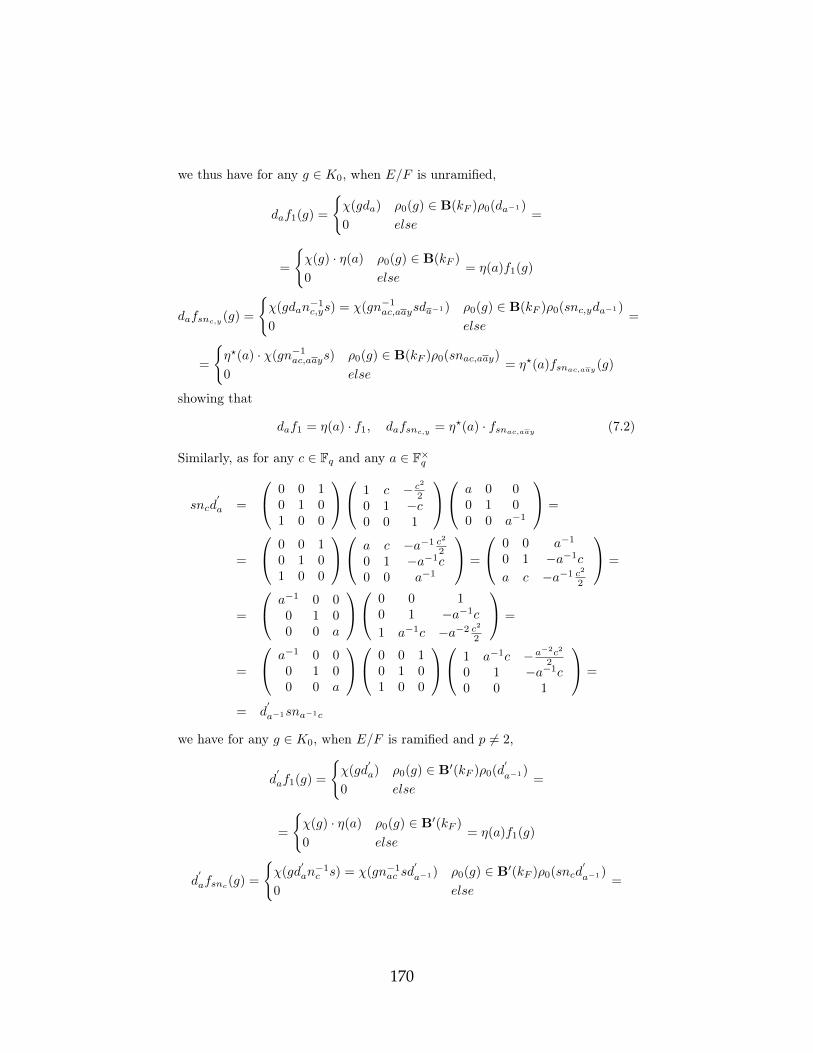
we thus have for any g ∈ K0, when E/F is unramified,

daf1(g) =

{χ(gda) ρ0(g) ∈ B(kF )ρ0(da−1)

0 else=

=

{χ(g) · η(a) ρ0(g) ∈ B(kF )

0 else= η(a)f1(g)

dafsnc,y (g) =

{χ(gdan

−1c,ys) = χ(gn−1

ac,aaysda−1) ρ0(g) ∈ B(kF )ρ0(snc,yda−1)

0 else=

=

{η?(a) · χ(gn−1

ac,aays) ρ0(g) ∈ B(kF )ρ0(snac,aay)

0 else= η?(a)fsnac,aay (g)

showing that

daf1 = η(a) · f1, dafsnc,y = η?(a) · fsnac,aay (7.2)

Similarly, as for any c ∈ Fq and any a ∈ F×q

sncd′a =

0 0 10 1 01 0 0

1 c − c220 1 −c0 0 1

a 0 00 1 00 0 a−1

=

=

0 0 10 1 01 0 0

a c −a−1 c2

20 1 −a−1c0 0 a−1

=

0 0 a−1

0 1 −a−1c

a c −a−1 c2

2

=

=

a−1 0 00 1 00 0 a

0 0 10 1 −a−1c

1 a−1c −a−2 c2

2

=

=

a−1 0 00 1 00 0 a

0 0 10 1 01 0 0

1 a−1c −a−2c2

20 1 −a−1c0 0 1

=

= d′

a−1sna−1c

we have for any g ∈ K0, when E/F is ramified and p 6= 2,

d′af1(g) =

{χ(gd

′a) ρ0(g) ∈ B′(kF )ρ0(d

′

a−1)

0 else=

=

{χ(g) · η(a) ρ0(g) ∈ B′(kF )

0 else= η(a)f1(g)

d′afsnc(g) =

{χ(gd

′an−1c s) = χ(gn−1

ac sd′

a−1) ρ0(g) ∈ B′(kF )ρ0(sncd′

a−1)

0 else=

170

=

{η−1(a) · χ(gn−1

ac s) ρ0(g) ∈ B′(kF )ρ0(snac)

0 else= η−1(a)fsnac(g)

showing thatd′af1 = η(a) · f1, d

′afsnc = η−1(a) · fsnac (7.3)

When p = 2 and E/F is ramified, we see that

sn0,yd′a =

0 0 10 1 01 0 0

1 0 y0 1 00 0 1

a 0 00 1 00 0 a−1

=

=

0 0 10 1 01 0 0

a 0 a−1y0 1 00 0 a−1

=

0 0 a−1

0 1 0a 0 a−1y

=

=

a−1 0 00 1 00 0 a

0 0 10 1 01 0 a−2y

=

=

a−1 0 00 1 00 0 a

0 0 10 1 01 0 0

1 0 a−2y0 1 00 0 1

=

= d′

a−1sn0,a−2y

so for any g ∈ K0

d′afsn0,y

(g) =

{χ(gd

′an−10,ys) = χ(gn−1

0,a2ysd′

a−1) ρ0(g) ∈ B′(kF )ρ0(sn0,yd′

a−1)

0 else=

=

{η−1(a) · χ(gn−1

0,a2ys) ρ0(g) ∈ B′(kF )ρ0(sn0,a2y)

0 else= η−1(a)fsn0,a2y

(g)

showing that d′afsn0,y

= η−1(a) · fsn0,a2y.

As nc,y 7→ nac,aay is bijective on N(kF ), we see that

OCda∑

n∈N(kF )

fsn = OCη?(a)∑

n∈N(kF )

fsn

As η(a) is a unit (note that η is a character of a finite group), we have

OCda∑

n∈N(kF )

fsn = OC∑

n∈N(kF )

fsn

Similarly, when E/F is ramified, we see that c 7→ ac and y 7→ a2y are bijectiveon Fq, hence

OCd′a

∑

c∈Fqfsnc = OCη−1(a)

∑

c∈Fqfsnc = OC

∑

c∈Fqfsnc

171

and when p = 2

OCd′a

∑

y∈Fqfsn0,y = OCη−1(a)

∑

y∈Fqfsn0,y = OC

∑

y∈Fqfsn0,y

Next, note that, for E/F unramified,

snc,ys =

y−1 −y−1c 10 −y−1y −c0 0 y

sny−1c,y−1

if (c, y) 6= (0, 0) (note that y = 0⇒ c = 0), and forE/F ramified, if p 6= 2,

sncs =

− 2c2

2c 1

0 −1 −c0 0 − c22

sn− 2

c

if c 6= 0. If E/F is ramified, and p = 2, we see that

sn0,ys =

y−1 0 10 −1 00 0 y

sn0,y−1

if y 6= 0.Hence we have for any g ∈ K0, for E/F unramified,

nb,zsfs(g) = fs(gnb,zs) =

{χ(gnb,z) ρ0(gnb,zs) ∈ B(kF )s

0 else=

=

{χ(g) ρ0(g) ∈ B(kF )

0 else= f1(g)

while for E/F ramified, p 6= 2,

nbsfs(g) = fs(gnbs) =

{χ(gnb) ρ0(gnbs) ∈ B′(kF )s

0 else=

=

{χ(g) ρ0(g) ∈ B′(kF )

0 else= f1(g)

and for E/F ramified, p = 2,

n0,zsfs(g) = fs(gn0,zs) =

{χ(gn0,z) ρ0(gn0,zs) ∈ B′(kF )s

0 else=

=

{χ(g) ρ0(g) ∈ B′(kF )

0 else= f1(g)

172

Further, for any (c, y) 6= (0, 0), when E/F is unramified,

nb,zsfsnc,y (g) = fsnc,y (gnb,zs) =

{χ(gnb,zsn

−1c,ys) ρ0(gnb,zs) ∈ B(kF )ρ0(snc,y)

0 else=

=

{χ(gnb,zsn

−1c,ys) ρ0(g) ∈ B(kF )ρ0(snc,ysn

−1b,z)

0 else=

=

χ

gn−1

? s

y−1 −y−1c 1

0 −y−1y −c0 0 y

−1 ρ0(g) ∈ B(kF )ρ0(sn?)

0 else

=

=

{η(y) · χ

(gn−1

? s)

ρ0(g) ∈ B(kF )ρ0(sn?)

0 else= η(y) · fsn?(g)

where n? = ny−1c−b,y−1+z+y−1bc

Similarly, for c 6= 0, when E/F is ramified, and p 6= 2,

nbsfsnc(g) = fsnc(gnbs) =

{χ(gnbsn

−1c s) ρ0(gnbs) ∈ B′(kF )ρ0(snc)

0 else=

=

{χ(gnbsn

−1c s) ρ0(g) ∈ B′(kF )ρ0(sncsn

−1b )

0 else=

=

χ

gn

−1− 2c−b

s

− 2c2

2c 1

0 −1 −c0 0 − c22

−1 ρ0(g) ∈ B′(kF )ρ0(sn−2c−1−b)

0 else

=

=

{η(− c22

)· χ(gn−1−2c−1−bs

)ρ0(g) ∈ B′(kF )ρ0(sn−2c−1−b)

0 else= η

(−c

2

2

)·fsn−2c−1−b(g)

and for y 6= 0, when E/F is ramified and p = 2,

n0,zsfsn0,y(g) = fsn0,y

(gn0,zs) =

{χ(gn0,zsn

−10,ys) ρ0(gn0,zs) ∈ B′(kF )ρ0(sn0,y)

0 else=

=

{χ(gn0,zsn

−10,ys) ρ0(g) ∈ B′(kF )ρ0(sn0,ysn

−10,z)

0 else=

173

=

χ

gn

−10,y−1+zs

y−1 0 1

0 −1 0

0 0 y

−1 ρ0(g) ∈ B′(kF )ρ0(sn0,y−1+z)

0 else

=

=

{η(y) · χ

(gn−1

0,y−1+zs)

ρ0(g) ∈ B′(kF )sn0,y−1+z

0 else= η(y) · fsn0,y−1+z

(g)

These show that for any nb,z ∈ N(kF ), when E/F is unramified,

nb,zsfs = f1, nb,zsfsnc,y = η(y) · fsny−1c−b,y−1+z+y−1bc(7.4)

and for any b ∈ Fq, when E/F is ramified, p 6= 2,

nbsfs = f1, nbsfsnc = η

(−c

2

2

)· fsn−2c−1−b (7.5)

while for any z ∈ Fq, when E/F is ramified, and p = 2,

n0,zsfs = f1, n0,zsfsn0,y= η(y) · fsn0,y−1+z

(7.6)

Therefore, for E/F unramified, we have

Fb,z = Fnb,z := nb,zs∑

nc,y∈N(kF )

fsnc,y = f1 +∑

06=nc,y∈N(kF )

η(y) · fsn? =

= f1 +∑

nc,y∈N(kF )

η?(y + z − bc)fsnc,y

where the character η? of F?q is extended to a function on Fq vanishing on 0.For E/F ramified, when p 6= 2, we have

Fb := Fnb = nbs∑

c∈Fqfsnc = f1 +

∑

06=c∈Fqη

(−c

2

2

)· fsn−2c−1−b =

= f1 +∑

c∈Fqη−1

(− (b+ c)2

2

)fsnc

and for E/F ramified with p = 2, we have

Fz := Fn0,z= n0,zs

∑

y∈Fqfsn0,y

= f1 +∑

06=y∈Fqη(y) · fsn0,y−1+z

=

= f1 +∑

y∈Fqη−1(y + z)fsn0,y

174

We have, combining with (7.2), when E/F is unramified

daFb,z = danb.zs∑

nc,y∈N(kF )

fsnc,y = η(a)f1+η?(a)∑

nc,y∈N(kF )

η?(y+z−bc)fsnac,aay =

= η(a)

f1 +

∑

nc,y∈N(kF )

η?(aay + aaz − aabc)fsnac,aay

=

= η(a)

f1 +

∑

nc,y∈N(kF )

η?(y + aaz − (ab)c)fsnc,y

= η(a) · Fab,aaz

As η(a) is a unit, we have

OCdanb,zs∑

nc,y∈N(kF )

fsnc,y = OCFab,aaz

Similarly, when E/F is ramified and p 6= 2, we have

d′aFb = d

′anbs

∑

c∈Fqfsnc = η(a)f1 + η−1(a)

∑

c∈Fqη−1

(− (b+ c)2

2

)fsnac =

= η(a)

f1 +

∑

c∈Fqη−1

(−a

2(b+ c)2

2

)fsnac

=

= η(a)

f1 +

∑

c∈Fqη−1

(− (ab+ c)2

2

)fsnc

= η(a) · Fab


OCd′anbs

∑

c∈Fqfsnc = OCFab

and when E/F is ramified with p = 2, we have

d′aFz = d

′an0,zs

∑

y∈Fqfsn0,y

= η(a)f1 + η−1(a)∑

y∈Fqη−1(y + z)fsn0,a2y

=

= η(a)

f1 +

∑

y∈Fqη−1

(a2(y + z)

)fsn0,a2y

=

= η(a)

f1 +

∑

y∈Fqη−1(y + a2z)fsn0,y

= η(a) · Fa2z

175


OCd′an0,zs

∑

y∈Fqfsn0,y

= OCFa2z

We deduce that M0 is the OC-module generated, when E/F is unramified, by∑

n∈N(kF )

fsn, (Fn)n∈N(kF )

when E/F is ramified, and p 6= 2, by∑

c∈Fqfsnc , (Fb)b∈Fq

and when E/F is ramified and p = 2, by∑

y∈Fqfsn0,y

, (Fz)z∈Fq

which is the statement.

With this in hand, we may complete the proof of the necessity of the criterion.

Proposition 7.12. Let χ : E× → C be a tamely ramified character, such thatindGBχ is integral. Let λ = χ(π). Then λq2 ∈ OC .

Proof. Consider the sum, when E/F is unramified,

∑

n∈N(kF )

Fn = q3/2f1 +∑

nc,y∈N(kF )

∑

nb,z∈N(kF )

η?(y + z − bc)

fsnc,y

We also note that nc,y · nb,z = ny+z,y+z−bc, hence we see that∑

nb,z∈N(kF )

η?(y + z − bc) =∑

nb,z∈N(kF )

η?(z)

By Lemma 2.24, we see that:If η is trivial, (the unramified case)

∑

nb,z∈N(kF )

Fb,z = q3/2f1 + (q3/2 − 1)∑

nc,y∈N(kF )

fsnc,y

If η �F×q1/26= 1, then

∑

nb,z∈N(kF )

Fb,z = q3/2f1

176

If η �Fq1/2

= 1 and p 6= 2, then for any i ∈ F−q∑

nb,z∈N(kF )

Fb,z = q3/2f1 − q1/2(q1/2 − 1)η(i) ·∑

nc,y∈N(kF )

fsnc,y

If η �Fq1/2

= 1 and p = 2, then

∑

nb,z∈N(kF )

Fb,z = q3/2f1 − q1/2(q1/2 − 1) ·∑

nc,y∈N(kF )

fsnc,y

In any case, we see that q3/2f1 ∈M0. Being K0-stable, by Proposition 7.3, M0

contains q3/2L0.By Lemma 7.10, the zigzag z(L0) = K0 · r0(r−1

1 (L1)) contains q1/2λM0, henceq2λL0.When E/F is ramified, we consider the sum

∑

b∈FqFb = qf1 +

∑

c∈Fq

∑

b∈Fqη−1

(− (b+ c)2

2

) fsnc

when p 6= 2 and the sum

∑

z∈FqFz = qf1 +

∑

y∈Fq

∑

z∈Fqη−1(y + z)

fsn0,y

when p = 2.Note that nb · nc = nb+c and n0,y · n0,z = n0,y+z. As b 7→ nb, z 7→ n0,z : kE →N′(kF ) are bijective, we see that

∑

b∈Fqη−1

(− (b+ c)2

2

)=∑

b∈Fqη−1

(−b

2

2

)

Also ∑

z∈Fqη−1(y + z) =

∑

z∈Fqη−1(z)

By Lemma 2.24, we see that:If η is either εq or trivial

∑

b∈FqFb = qf1 + η

(−1

2

)· (q − 1) ·

∑

c∈Fqfsnc

else ∑

b∈FqFb = qf1

177

Further, when p = 2, we have if η = 1

∑

z∈FqFz = qf1 + (q − 1) ·

∑

y∈Fqfsn0,y

else ∑

z∈FqFz = qf1

In any case, we see that qf1 ∈ M0. Being K0-stable, by Proposition7.3, M0

contains qL0.By Lemma 7.10, the zigzag z(L0) = K0 · r0(r−1

1 (L1)) contains qλM0, henceq2λL0.Thus in all cases, z(L0) contains q2λL0.If the sequence of zigzags (zn(L0))n≥0 is finite, then q2λ ∈ OC . By Corollary6.18, if q2λ /∈ OC , then indGBχ is not integral.

Corollary 7.13. This shows that for indGPχ to be integral, we must have 1 ≤|λ| ≤ |q−2|.

Remark 7.14. Note that by Corollary 6.21, as the contragredient representationof indGBχ is indGBχ

−1ω2, and χ−1ω2(π) = λ−1q−2, we see that if indGBχ isintegral, so is indGBχ

−1ω2, showing that 1 ≤∣∣λ−1q−2

∣∣ ≤ |q−2|, hence 1 ≤ |λ| ≤|q−2|. This shows that our condition is compatible with Corollary 6.21.It is also compatible with the isomorphism indGBχ ' indGBχ

?ω2 by the samecomputation.

7.3. Proof of sufficiency

We have established the necessity of the condition, and turn now to sufficiency.We assume, then, that λ−1 ∈ OC and q2λ ∈ OC . Further, by Corollary 7.8, wemay assume λ /∈ OC .To go further, we need a Lemma.

Definition 7.15. For a function a : Fq → OC and a character η : F×q → O×C ,we consider the convolution of a with η, denoted by a ∗ η, and defined by

(a ∗ η)(y) :=∑

z∈Fqa(−z)η(y + z)

for all y ∈ Fq, where we set η(0) := 0.

Definition 7.16. We say that a ∗ η is constant modulo λ−1OC if there existssome c ∈ C such that (a ∗ η)(y)− c ∈ λ−1OC for all y ∈ Fq.

Lemma 7.17.∑z∈Fq a(z) ∈ q ·OC+λ−1 ·OC if a∗η is constant modulo λ−1OC .

178

Proof. When the character η is trivial, the function a ∗ η + a =∑z∈Fq a(z) is

constant. If a ∗ η is constant modulo λ−1OC , so is a, and∑

z∈Fqa(z) ∈ q · a(0) + λ−1OC ⊂ q · OC + λ−1 · OC

When the character η is not trivial, we use the Fourier transform. We replaceC by a finite extension in order to find a non-trivial character ψ : Fq → OC todefine the Fourier transform

f(y) =∑

z∈Fqψ(zy)f(z)

of a function f : Fq → C.

We denote by R the space of integral functions f : Fq → OC , by R the imageof R by Fourier transform, by δ0 ∈ R the characteristic function of 0, and by∆ ∈ R the constant function ∆(y) = 1.The properties of the Fourier transform yield

ˆf = qf, ∆ = qδ0, δ0 = ∆, η(0) = 0

η(x) is a Gauss sum, and η(x)η−1(x) = qη(−1) if x ∈ F×q . The Fourier transformof a convolution product f ∗ g is the product of the Fourier transforms, i.e.

f ∗ g = f · g

The lemma then states that a(0) ∈ (q+ λ−1)OC for all a ∈ R such that a ∗ η ∈OC∆ + λ−1R. By Fourier transform a ∗ η ∈ OC∆ + λ−1R is equivalent toa · η ∈ OCqδ0 + λ−1R. Multiplying by η−1, which vanishes only at zero, yieldsfor nonzero elements

qa = qa(0)δ0 + λ−1η−1 · φfor some φ ∈ R. The function b = qa belongs to qR. We have b = b(0)δ0 +

λ−1η−1 · φ and by Fourier transform b = β∆ + λ−1 · η−1 ∗ φ where b(0) =β + λ−1 · (η−1 ∗ φ)(0), hence β ∈ (q + λ−1) · OC . But a(0) = β, hence theresult.

We return to the proof of Theorem 7.1. By Lemma 7.9, the OC-module L′1 =

K1 · r1(r−10 (L0)) = K1 · (OCr1(φ1) +OCr1(φs)) is spanned over OC by

{Hz}z∈F−q , r1(φ1), {λ−1htn0,π−1z}z∈F−q , λ

−1h1

if E/F is unramified, or by

{Hz}z∈Fq , r1(φ1), {λ−1htn0,π−1z}z∈Fq , λ−1h1

if E/F is ramified.

179

The OC-module r−11 (L

′1) = (L

′1)I(1) is spanned over OC by (λ−1L1)I(1), φ1, and,

when E/F is unramified, by linear combinations (we let i ∈ F−q be arbitrary)

∑

z∈F−q

a(−z/i)Hz =

∑

z∈Fq1/2

a(−z)

· ht +

∑

z∈Fq1/2

a(−z)η?(zi)

· h1 +

+∑

06=y∈F−q

∑

z∈Fq1/2

a(−z)η?(1 + yzi)

htn0,π−1y

=

= a(0)·ht+(a∗η?)(0)·η?(i)·h1+η?(i)·∑

06=y∈F−q

η?(y)·(a∗η?)(i−1y−1)·htn0,π−1y=

= a(0) · ht + (a ∗ η?)(0) · η?(i) · r1(φ1)

for all functions a : Fq1/2 → OC such that a ∗ η∗ is constant modulo λ−1OC ,where η? is identified with its restriction on F×

q1/2 .

When E/F is ramified, it is spanned by linear combinations

∑

z∈Fqa(−z)Hz =

∑

z∈Fqa(−z)

· ht +

∑

z∈Fqa(−z)η−1(z)

· h1 +

+∑

06=y∈Fq

∑

z∈Fqa(−z)η−1(1 + yz)

htn0,π−1y

=

= a(0) · ht + (a ∗ η−1)(0) · h1 +∑

0 6=y∈Fqη−1(y) · (a ∗ η−1)(y−1) · htn0,π−1y

=

= a(0) · ht + (a ∗ η−1)(0) · η−1(i) · r1(φ1)

for all functions a : Fq → OC such that a ∗ η−1 is constant modulo λ−1OC .As (a ∗ η?)(0) ∈ OC and a(0) ∈ q1/2 · OC + λ−1 · OC by Lemma 7.17, we obtainwhen E/F is unramified that

r−11 (L

′1) = OCφ1 + (q1/2λ · OC +OC) · φs

When E/F is ramified, as (a ∗ η?)(0) ∈ OC and a(0) ∈ q · OC + λ−1 · OC byLemma 7.17, we obtain

r−11 (L

′1) = OCφ1 + (qλ · OC +OC) · φs

Note that when E/F is unramified, if q1/2λ ∈ OC , i.e. |λ| ≤∣∣q−1/2

∣∣, we arealready done, as r−1

1 (L′1) = r−1

0 (L0) = OCφ1 +OCφs.Similarly, when E/F is ramified, if qλ ∈ OC , i.e. |λ| ≤ |q−1|, we are also done,as r−1

1 (L′1) = r−1

0 (L0) = OCφ1 +OCφs.

180

Assume, if so, in the case E/F unramified, that q1/2λ /∈ OC , so that r−11 (L

′1) =

OCφ1 + q1/2λOCφs, and in the case E/F ramified, that qλ /∈ OC , so thatr−11 (L

′1) = OCφ1 + qλOCφs. Then if E/F is unramified,

z(L0) = K0 ·

OCf1 + q1/2λOC ·

∑

n∈N(kF )

fsn

= L0 + q1/2λM0

is the OC-module spanned over OC by (see Proposition 7.11)

L0, q1/2λ ·

∑

n∈N(kF )

fsn,(q1/2λ · Fn

)n∈N(kF )

while if E/F is ramified,

z(L0) = K0 ·

OCf1 + qλOC ·

∑

n∈N′(kF )

fsn

= L0 + qλM0

is the OC-module spanned over OC by (see Proposition 7.11)

L0, qλ ·∑

n∈N′(kF )

fsn, (qλ · Fn)n∈N′(kF )

The OC-module r−10 (z(L0)) = (z(L0))I(1) is spanned, when E/F is unramified,

over OC by LI(1)0 , q1/2λφs and by the preimages of

∑

nb,z∈N(kF )

a(−b, z) · Fb,z =

∑

nb,z∈N(kF )

a(−b, z)

· f1 +

+∑

nc,y∈N(kF )

∑

nb,z∈N(kF )

a(−b, z) · η?(y + z − bc)

fsnc,y

for all functions a : FNq → q1/2λOC such that (c, y) 7→ ∑nb,z∈N(kF ) a(−b, z) ·

η?(y + z − bc) is constant modulo OC .When E/F is ramified, and p 6= 2, it is spanned over OC by LI(1)

0 , qλφs and bythe preimages of

∑

b∈Fqa(−b) ·Fb =

∑

b∈Fqa(−b)

· f1 +

∑

c∈Fq

∑

b∈Fqa(−b) · η−1

(− (b+ c)2

2

) fsnc

for all functions a : Fq → qλOC such that c 7→ ∑b∈Fq a(−b) · η−1

(− (b+c)2

2

)is

constant modulo OC .

181

When E/F is ramified and p = 2, it is spanned over OC by LI(1)0 , qλφs and by

the preimages of

∑

z∈Fqa(−z) · Fz =

∑

z∈Fqa(−z)

· f1 +

∑

y∈Fq

∑

z∈Fqa(−z) · η−1 (y + z)

fsny

for all functions a : Fq → qλOC such that y 7→ ∑z∈Fq a(−z) · η−1 (y + z) is

constant modulo OC .Definition 7.18. Let us now define for any two functions a, θ : N(kF ) → Cthe convolution of a with θ, which is the function a ∗ θ : N(kF )→ C defined by

(a ∗ θ)(x) =∑

n∈N(kF )

a(n−1) · θ(xn)

Or more explicitly

(a ∗ η)(nc,y) :=∑

nb,z∈N(kF )

a(n−b,z) · θ(nb+c,y+z−bc)

This convolution operation is associative, since for any x ∈ N(kF ) we have

((a∗θ)∗ϑ)(x) =∑

n∈N(kF )

(a∗θ)(n−1)·ϑ(xn) =∑

n∈N(kF )

∑

y∈N(kF )

a(y−1)·θ(n−1y−1)·ϑ(xn) =

=∑

y∈N(kF )

a(y−1)·∑

n∈N(kF )

θ(n−1)·ϑ(xyn) =∑

y∈N(kF )

a(y−1)·(θ∗ϑ)(xy) = (a∗(θ∗ϑ))(x)

It is also clearly C-bilinear.Similarly, we define a convolution on N′(kF ) in the same manner.

Definition 7.19. For a character η : F×q → O×C , we extend it to a functionη : Fq → OC by setting η(0) := 0, and define a function η : N(kF ) → C bysetting for any nb,z ∈ N(kF )

η(nb,z) = η(z)

If E/F is ramified, we define η(nb) = − b22 if p 6= 2, and η(n0,z) = η(z) if p = 2.

Before we prove a similar proposition for this case, we prove a little lemma.

Lemma 7.20. Assume η 6= 1. Then for any 1 6= n ∈ N(kF ), we have, if E/Fis unramified,

(η ∗ η?)(n) =

−1 η �Fq1/26= 1

−q1/2(q1/2 − 1)η?(i) · η(n)− 1 η �Fq1/2

= 1, p 6= 2

−q1/2(q1/2 − 1)η(n)− 1 η �Fq1/2

= 1, p = 2

182

and if E/F is ramified, and p 6= 2,

(η ∗ ˜η−1)(n) =

−1 η 6= εq, 1, n 6= 1

q − 2 η = εq, 1, n 6= 1

q − 1 n = 1

Proof. Before we proceed, we note that for any z ∈ Fq , as the norm mapFq → Fq1/2 is surjective, there exists b ∈ Fq such that bb = −(z + z).Moreover, if z ∈ F−q , it follows that b = 0 is the only possible value for b, andelse, we have

∣∣F1q

∣∣ = q1/2 + 1 different solutions for this equation.

If (c, y) 6= (0, 0), in particular y 6= 0, so we may consider the setA ={zy | z ∈ F−q

}=

1y · F−q .For any a ∈ Fq, if 1 6= a /∈ A, then a · y /∈ F−q , hence a · y + a · y 6= 0, so thereexist q + 1 different values of d ∈ Fq such that dd = −a · y − a · y.For each such value, we let b = c+d

a−1 , which is well defined since a 6= 1, and

z = y−bca−1 . Then

1 +y − bcz

= a

z+z+bb =1

(a− 1)(a− 1)·(y(a− 1)− c(c+ d) + y(a− 1)− c(c+ d) + (c+ d)(c+ d)

)=

=ay + ay − y − y − 2cc− cd− cd+ cc+ cd+ cd+ dd

(a− 1)(a− 1)=

=(ay + ay + dd)− (y + y + cc)

(a− 1)(a− 1)= 0

If 1 6= a ∈ A, then we see that there exists a unique such value of d, and b, z arechosen once more in the same way.For a = 1, we seek solutions for y− bc = 0. In such a case, we have either c = 0(equivalently, y ∈ F−q or 1 ∈ A), when we do not have any solutions, or c 6= 0

(equivalently, y /∈ F−q or 1 /∈ A), when b = yc yields q1/2 solutions. This shows

that when c = 0

∑

16=nb,z∈N(kF )

η?(

1 +y − bcz

)=

∑

16=a∈Aη?(a) + (q1/2 + 1) ·

∑

a/∈Aη?(a) =

=

(∑

a∈Aη?(a) + (q1/2 + 1) ·

∑

a/∈Aη?(a)

)− 1

and when c 6= 0

∑

1 6=nb,z∈N(kF )

η?(

1 +y − bcz

)=∑

a∈Aη?(a)+q1/2 ·η?(1)+(q1/2+1)·

∑

16=a/∈Aη?(a) =

183

=

(∑

a∈Aη?(a) + (q1/2 + 1) ·

∑

a/∈Aη?(a)

)− 1

We note that∑a∈A η

?(a) = η(y) ·∑a∈F−q η?(a), so in any case we are interested

in computing the value of

η(y) ·

∑

a∈F−q

η?(a) + (q1/2 + 1) ·∑

a/∈F−q

η?(a)

− 1

Now, we have already seen in Lemma2.24, that if η �Fq1/2

= 1,∑a∈F−q η

?(a) =

q1/2 · η?(i) if p 6= 2 and q if p = 2, while if η �Fq1/26= 1,

∑a∈F−q η

?(a) = 0.

Note also that∑a/∈F−q η

?(a) = −∑a∈F−q η?(a), since η 6= 1 is nontrivial. There-

fore, if η �Fq1/2

= 1, then

(η∗η?)(nc,y) = η(y)·

−q ·

∑

a∈F−q

η?(a)

−1 =

{−q1/2(q1/2 − 1)η?(i) · η(y)− 1 p 6= 2

−q1/2(q1/2 − 1)η(y)− 1 p = 2

Next, consider the case E/F is ramified and p 6= 2. Then, as for any c 6= 0, themap b 7→ 1 + c

b is bijective F×q → Fq\{1}, we see that for c 6= 0

(η ∗ ˜η−1)(nc) =∑

06=b∈Fqη−1

((1 +

c

b

)2)

=∑

1 6=x∈Fqη−1

(x2)

and by Lemma 2.24, it follows that

(η ∗ ˜η−1)(nc) =

{−1 η 6= εq, 1

q − 2 η = εq, 1

When c = 0, we see that (η ∗ ˜η−1)(1) =∑b∈F×q η

−1 (1) = q − 1.

This concludes the proof of the lemma.

We shall prove the following proposition.

Proposition 7.21. When E/F is unramified,∑n∈N(kF ) a(n) ∈ OC if a ∗ η is

constant modulo OC . When E/F is ramified,∑n∈N′(kF ) a(n) ∈ OC if a ∗ η is

constant modulo OC .

Proof. When E/F is ramified and p = 2, this is the result of Lemma 7.17. Fromnow on, when E/F is ramified, we assume p 6= 2.When the character η is trivial, the function a ∗ η + a =

∑n∈N(kF ) a(n) is

constant. If a ∗ η is constant modulo OC , so is a, and∑

n∈N(kF )

a(n) ∈ q3/2a(1) +OC ⊂ q2λOC +OC ⊂ OC

184

Similarly, when E/F is ramified, and η = εq or trivial, the function a ∗ η + a =∑n∈N′(kF ) a(n) is constant. If a ∗ η is constant modulo OC , so is a, and

∑

n∈N′(kF )

a(n) ∈ qa(1) +OC ⊂ q2λOC +OC ⊂ OC

This settles the case of χ unramified. We turn to the tamely ramified case. IfE/F is ramified, we may further assume µ 6= εq.We denote by R the space of integral functions N(kF ) → OC , by δ0 ∈ R thecharacteristic function of 0, and by ∆ ∈ R the constant function ∆ = 1.Then, when E/F is unramified, we have a ∈ q1/2λR such that a∗ η ∈ C ·∆+R,hence there exist α ∈ C and φ ∈ R such that

a ∗ η = α∆ + φ (7.7)

When E/F is ramified, we have that a ∈ qλR. Let us convolve by η? whenE/F is unramified, or by ˜η−1 when E/F is ramified. Note that we have thefollowing identities

(η ∗ η?)(nc,y) =∑

nb,z∈N(kF )

η(z) · η?(y + z − bc) =

=∑

16=nb,z∈N(kF )

η?(y + z − bc

z

)=

∑

16=nb,z∈N(kF )

η?(

1 +y − bcz

)

(η ∗ ˜η−1)(nc) =∑

b∈Fqη

(−b

2

2

)· η−1

(− (b+ c)2

2

)=

∑

06=b∈Fqη−1

((1 +

c

b

)2)

It follows that when E/F is unramified, (η ∗ η?)(1) = |N(kF )| − 1 = q3/2 − 1,and when E/F is ramified, (η ∗ ˜η−1)(1) = q − 1 (see Lemma 2.23).Now, by Lemma 7.20 for η : F×q → C, one has when E/F is unramified

η ∗ η? =

q3/2 · δ0 −∆ η �Fq1/26= 1

q3/2 · δ0 −∆− q1/2(q1/2 − 1)η?(i) · η η �Fq1/2

= 1, p 6= 2

q3/2 · δ0 −∆− q1/2(q1/2 − 1) · η η �Fq1/2

= 1, p = 2


η ∗ ˜η−1 = q · δ0 −∆

Therefore, when E/F is unramified, if η �Fq1/26= 1, from (7.7) we have

q3/2 · (a ∗ δ0)− (a ∗∆) = a ∗ (q3/2 · δ0 −∆) = a ∗ (η ∗ η?) =

= (a ∗ η) ∗ η? = (α ·∆ + φ) ∗ η? = α ·(∆ ∗ η?

)+ φ ∗ η?

185

and if E/F is ramified, we have

q · (a ∗ δ0)− (a ∗∆) = a ∗ (q · δ0 −∆) = a ∗ (η ∗ ˜η−1) =

= (a ∗ η) ∗ ˜η−1 = (α ·∆ + φ) ∗ η? = α ·(

∆ ∗ ˜η−1)

+ φ ∗ ˜η−1

However, note that for any function a, one has when E/F is unramified

(a ∗ δ0)(nc,y) =∑

nb,z∈N(kF )

a(n−b,z) · δ0(nb+c,y+z−bc) = a(nc,y)⇒ a ∗ δ0 = a


(a ∗ δ0)(nc) =∑

b∈Fqa(n−b) · δ0(nb+c) = a(nc)⇒ a ∗ δ0 = a

Furthermore, when E/F is unramified, we have

(a∗∆)(nc,y) =∑

n∈N(kF )

a(n) = (∆∗a)(nc,y)⇒ a∗∆ = ∆∗a =

∑

n∈N(kF )

a(n)

·∆


(a ∗∆)(ny) =∑

b∈Fqa(nb) = (∆ ∗ a)(nc)⇒ a ∗∆ = ∆ ∗ a =

∑

b∈Fqa(nb)

·∆

In particular, if a = η is inflated from some character, and E/F is unramified,then ∑

nb,z∈N(kF )

η(z) =∑

z∈F−q

η(z) + (q + 1) ·∑

z/∈F−q

η(z) =

=

0 η �Fq1/26= 1

−q1/2(q1/2 − 1)η(i) η �Fq1/2

= 1, p 6= 2

−q1/2(q1/2 − 1) η �Fq1/2

= 1, p = 2

if a = η, but E/F is ramified, then

∑

b∈Fqη

(−b

2

2

)= 0

Therefore, subtituiting, we obtain, when η �Fq1/26= 1, that if E/F is unramified

q3/2a−

∑

n∈N(kF )

a(n)

·∆ = φ ∗ η? ∈ R

186

and if E/F is ramified

qa−

∑

b∈Fqa(nb)

·∆ = φ ∗ ˜η−1 ∈ R

However, as a ∈ q1/2λR when E/F is unramified, we see that q3/2a ∈ q2λR ⊂R, hence ∑n∈N(kF ) a(n) ∈ OC , as required.Also, as a ∈ qλR when E/F is ramified, we see that qa ∈ q2λR ⊂ R, hence∑b∈Fq a(nb) ∈ OC , as required.

Similarly, if η �Fq1/2

= 1, we obtain from (7.7) either

q3/2a−

∑

n∈N(kF )

a(n)

·∆− q1/2(q1/2 − 1) · (a ∗ η) =

= a ∗ (q3/2 · δ0 −∆− q1/2(q1/2 − 1) · η) =

= α ·(∆ ∗ η?

)+ φ ∗ η? = −q1/2(q1/2 − 1)α ·∆ + φ ∗ η?

in the case p = 2, which after resubtituting, becomes

q3/2a−

∑

n∈N(kF )

a(n)

·∆− q1/2(q1/2 − 1)φ = φ ∗ η?

or

q3/2a−

∑

n∈N(kF )

a(n)

·∆− q1/2(q1/2 − 1)η?(i) · (a ∗ η) =

= −q1/2(q1/2 − 1)η?(i) · α ·∆ + φ ∗ η?

in the case p 6= 2, which after resubtituting, becomes

q3/2a−

∑

n∈N(kF )

a(n)

·∆− q1/2(q1/2 − 1)η?(i) · φ = φ ∗ η?

In any case, by the same argument, since q1/2(q1/2−1), η?(i) ∈ OC , we see that∑n∈N(kF ) a(n) ∈ OC , as required.

Corollary 7.22. If λ−1 ∈ OC , q2λ ∈ OC , then indGBχ is integral.

Proof. Returning to the OC-module r−10 (z(L0)) = (z(L0))I(1), we see that it is

generated by φ1, q1/2λφs and by ∑

n∈N(kF )

a(n−1)

· φ1 + (a ∗ η?)(0) · φs

187

for all functions a : N(kF ) → q1/2λOC such that a ∗ η? is constant moduloOC . For such functions, by Proposition 7.21, we have

∑n∈N(kF ) a(n) ∈ OC

, hence the above functions already belong to OCφ1 + q1/2λOCφs, showingthat r−1

0 (z(L0)) = OCφ1 + q1/2λOCφs = r−1(L1), hence the coefficient systemcorresponding to z(L0), L1 yields an integral structure in indGBχ, by Corollary6.16.

Remark 7.23. (i) In Theorem 7.1, χ(π) is a unit if and only if the characterχ ⊗ χ1 of M is OC-integral. By Corollary 7.8, in this case, L is the naturalOC-integral structure of functions in indGB(χ ⊗ χ1) with values in OC . Thereduction of L is the kC-principal series of G induced from the reduction χ⊗χ1

of χ⊗ χ1.(ii) The unimodular character of P is δ(p) = ω(a)2, where ω(π) = 1/q2. Thecontragredient of indGB(χ⊗χ1) is indGB(χ−1 ·ω2⊗χ−1

1 ), hence Theorem 7.1 andCorollary 6.21 are compatible.

Let χ0(t) = χ(t)χ1(tt−1

). Then D. Keys showed in Keys [18] that the represen-tation

indGB(χ⊗ χ1) ' indGB(χ?ω2 ⊗ χ1)

is reducible only when either χ0 = 1, ω2, or χ0 ∈{ηω1/2, ηω3/2

}and η �F×=

ηE/F , or χ0 �F×= ω but χ0 6= ω. The isomorphism is compatible with Theorem7.1(iii) Theoretically, there is no reason to restrict to the tamely ramified smoothcase, but the computations become harder when the level increases or when oneadds an algebraic part.(iv) One should see c) as the limit at ∞ of the integrality local criterion.

8. Application to reduction and k-representations

8.1. Reduction.

An R-integral finitely generated S-representation V of G contains an R-integralstructure Lft which is finitely generated as an RG-module; two finitely gener-ated R-integral structures Lft, L

′ft of V are commensurable: there exists a ∈ R

non zero such that aLft ⊂ L′ft, aL

′ft ⊆ Lft.

Let x be a uniformizer of R and k = R/xR. When the reduction Lft := Lft/xLftis a finite length kG-module, the reduction L of an R-integral structure L ofV commensurable to Lft has finite length and the same semi-simplification asLft.

Lemma 8.1. If the reduction Lft is an irreducible k-representation of H, thenthe R-integral structures of V are the multiples of Lft.

188

Proof. Let L be an integral structure of V which is different from Lft. Takinga multiple of Lft, we reduce to Lft ⊂ L and Lft not contained in xL. Theinclusions

xLft ⊂ (xL ∩ Lft) ⊂ Lftthe right one being strict, and the irreducibility of Lft/xLft imply xL ∩ Lft =xLft, equivalent to L = Lft because there exists no v ∈ L and v /∈ Lft suchthat v ∈ x−1Lft.

In the integrality criterion (Proposition 6.13), when the properties of 2) are true,the reduction of the R-integral structure H0(L) of the S-representation H0(V)of G is the 0-th homology of the G-equivariant coefficient system defined by thediagram

L0

L01

>>

L1

We have the exact sequence of SG-modules:

0→ indGI V01 → indGK1V1 ⊕ indGK0

V0 → H0(V)→ 0

of free RG-modules:

0→ indGI L01 → indGK1L1 ⊕ indGK0

L0 → H0(L)→ 0

of kG-modules:

0→ indGI L01 → indGK1L1 ⊕ indGK0

L0 → H0(L)→ 0

8.2. k-representations of G.

Let k be a finite field of characteristic p. Consider an irreducible principal seriesof G over k. It can be written as indGB(χ⊗ χ1) for some lifts χ, χ1.By Theorem 7.1, Remark 7.23 (i), and Lemma 8.1, it follows that each OC-integral structure of indGB(χ⊗χ1) is a multiple of L which is defined in Remark7.23 (i).Therefore, an irreducible principal series of G over k is the 0-th homology of aG-equivariant coefficient system.Let µ⊗ µ1 be a k-character of M ; its restriction to M(OE) is the inflation of a

k-character η⊗η1 ofM(Fq). As before,(ind

G(Fq)B(Fq) (η ⊗ η1)

)N(Fq)= C ·φ1⊕C ·φs

where φ1, φs have supportB(Fq), B(Fq)sN(Fq) and value 1 at id, s, respectively.

189

Proposition 8.2. The principal series indGB(µ ⊗ µ1) is the 0-th homology ofthe G-equivariant coefficient system defined by the tamely ramified diagram

(indGB(µ⊗ µ1)

)K0(1)

(indGB(µ⊗ µ1)

)I(1)

55

))(indGB(µ⊗ µ1)

)K1(1)

inflated from the inclusions

(ind


)N(Fq)→ ind


(ind

H(Fq)M(Fq)Z(Fq)(η ⊗ η1)

)Z(Fq)→ ind

H(Fq)M(Fq)Z(Fq)(η ⊗ η1)

Proof. Let µ ⊗ µ1 : M → k× be a continuous character. There exists a mod-erately ramified continuous character χ ⊗ χ1 : M → O×C lifting µ ⊗ µ1. ApplyTheorem 7.1 and Remark 7.23 (i).

[1] Ramla Abdellatif. Autour des représentations modulo p des groupes ré-ductifs p-adiques de rang 1. PhD thesis, Université Paris Sud-Paris XI,2011.

[2] Peter Abramenko and Gabriele Nebe. Lattice chain models for affine build-ings of classical type. Mathematische Annalen, 322(3):537–562, 2002.

[3] Eran Assaf, David Kazhdan, and Ehud de Shalit. Kirillov models and thebreuil-schneider conjecture for GL2(F ). arXiv preprint arXiv:1302.3060,2013.

[4] Laure Barthel, Ron Livne, et al. Irreducible modular representations ofGL2 of a local field. Duke Mathematical Journal, 75(2):261–292, 1994.

[5] Christophe Breuil. The emerging p-adic langlands programme. In Pro-ceedings of the international congress of mathematicians, volume 2, pages203–230, 2010.

[6] Christophe Breuil and Peter Schneider. First steps towards p-adic lang-lands functoriality. Journal für die reine und angewandte Mathematik(Crelles Journal), 2007(610):149–180, 2007.

190

[7] François Bruhat and Jacques Tits. Groupes réductifs sur un corps local.Publications mathématiques de l’IHES, 41(1):5–251, 1972.

[8] Ana Caraiani, Matthew Emerton, Toby Gee, David Geraghty, VytautasPaskunas, and Sug Woo Shin. Patching and the p-adic local langlandscorrespondence. arXiv preprint arXiv:1310.0831, 2013.

[9] Marco De Ieso. Existence de normes invariantes pour GL2. Journal ofNumber Theory, 133(8):2729–2755, 2013.

[10] Matthew Emerton. Locally analytic vectors in representations of locallyp-adic analytic groups. arXiv preprint math/0405137, 2004.

[11] Matthew Emerton et al. p-adic L-functions and unitary completions ofrepresentations of p-adic reductive groups. Duke Mathematical Journal,130(2):353–392, 2005.

[12] William Fulton and Joe Harris. Representation theory, volume 129.Springer Science & Business Media, 1991.

[13] Paul B Garrett. Buildings and classical groups. CRC Press, 1997.

[14] Elmar Große-Klönne. On the universal module of p-adic spherical heckealgebras. American Journal of Mathematics, 136(3):599–652, 2014.

[15] Yongquan Hu. Normes invariantes et existence de filtrations admissibles.Journal für die reine und angewandte Mathematik (Crelles Journal), 2009(634):107–141, 2009.

[16] Jens C Jantzen. First cohomology groups for classical lie algebras. In Rep-resentation theory of finite groups and finite-dimensional algebras, pages289–315. Springer, 1991.

[17] Shin-ichi Kato. On eigenspaces of the hecke algebra with respect to a goodmaximal compact subgroup of a p-adic reductive group. MathematischeAnnalen, 257(1):1–7, 1981.

[18] David Keys. Principal series representations of special unitary groups overlocal fields. Compositio mathematica, 51(1):115–130, 1984.

[19] Karol Koziol and Peng Xu. Hecke modules and supersingular representa-tions of U (2, 1). arXiv preprint arXiv:1204.1273, 2012.

[20] Vytautas Paskunas. Coefficient systems and supersingular representationsof GL2(F ). arXiv preprint math/0403240, 2004.

[21] Peter Schneider and Ulrich Stuhler. Representation theory and sheaveson the bruhat-tits building. Publications Mathématiques de l’IHÉS, 85(1):97–191, 1997.

191

[22] Peter Schneider and Jeremy Teitelbaum. Locally analytic distributions andp-adic representation theory, with applications to GL2. Journal of theAmerican Mathematical Society, 15(2):443–468, 2002.

[23] Peter Schneider, Jeremy Teitelbaum, and Dipendra Prasad. U(g)-finitelocally analytic representations. Representation Theory of the AmericanMathematical Society, 5(5):111–128, 2001.

[24] Peter Schneider, Jeremy Teitelbaum, Das Uferlose, and das Leben Stür-mende. Banach-hecke algebras and p-adic galois representations. Doc.Math, pages 631–684, 2006.

[25] Claus M Sorensen. A proof of the breuil-schneider conjecture in the inde-composable case. Annals of Mathematics, 177:1–16, 2013.

[26] Jacques Tits. Représentations linéaires irréductibles d’un groupe réductifsur un corps quelconque. Journal für die reine und angewandte Mathe-matik, 247:196–220, 1971.

[27] Jacques Tits. Reductive groups over local fields. In Automorphic forms,representations and L-functions (Proc. Sympos. Pure Math., Oregon StateUniv., Corvallis, Ore., 1977), Part, volume 1, pages 29–69, 1979.

[28] Marie-France Vignéras. Representations modulaires des groupes reductifsp-adiques. Representations cuspidales de GL(n), volume 137. Springer,1996.

[29] Marie-France Vignéras. A criterion for integral structures and coefficientsystems on the tree of PGL(2, F ). Pure and Applied Mathematics Quar-terly, 4(4), 2008.

192

ניתן לסווג את הבעיות בהן עוסקת . אנו מוכיחים מספר מקרים פרטיים של ההשערה, בעבודה זו

הוכחת קיום נורמה אינוריאנטית בהצגות אלגבריות מקומית –עבודה זו לשני נושאים קשורים

והוכחת קיום נורמה אינוריאנטית בהצגות אלגבריות , מימעל שדה מקו GL(2)של החבורה

. מעל שדה מקומי U(3)) הלא מפוצלת(מקומית של החבורה

אנו מבצעים , בשיטה אחת –השיטות בהן נעשה שימוש בעבודה זו גם הן מתחלקות לשני סוגים

-עץ ברוהאהומולגיה של בעוד שהשיטות האחרות נעזרות ב, אדית-pרדוקציה לבעיה באנליזה . Gהחבורה טיטס של

GL(2)אנו מוכיחים את קיומה של נורמה אינוריאנטית בהצגות אלגבריות מקומית של , 2בפרק

, עבור הצגות לא מסועפות ממשקל קטן, שניידר-מעל שדה מקומי כאשר מתקיים קריטריון בריי

הן הוכחו בשיטות , למרות ששתי התוצאות היו ידועות בעבר. והצגות מסועפות במתינות וחלקות .שונות וזו השיטה הראשונה שמוכיחה את שתיהן יחד

GL(2)אנו מוכיחים את קיומה של נורמה אינוריאנטית בהצגות אלגבריות מקומית של , 3בפרק

עבור חלק מההצגות הלא מסועפות , שניידר-מעל שדה מקומי כאשר מתקיים קריטריון בריי

אך , יש כאן הגבלה טכנית שלא הצלחנו להסיר, משקלמעבר להגבלה על ה. ממשקל גבוה יותר .אנו מעריכים שהיא טכנית בלבד

U(3)אנו מוכיחים את קיומה של נורמה אינוריאנטית בהצגות אלגבריות מקומית של , 4בפרק

, עבור הצגות לא מסועפות ממשקל קטן, שניידר-מעל שדה מקומי כאשר מתקיים קריטריון בריי .הדבר נעשה בשיטות שונות עבור כל אחד מהמקרים. נות וחלקותוהצגות מסועפות במתי

.אף אחד מהפרקים עדיין לא פורסם

תקציראת הבנתנו לגבי בעיות להעמיקשמטרתה , אדית-pתכנית לנגלנדס ה הינה חלק מו עבודה ז

מחקר עקומים אליפטיים ויריעות , כמו פתרון משוואות דיופנטיות, יסודיות בתורת המספרים

מכוונת ליצירת התאמה בין הצגות מסוימות של חבורות גלואה לבין לנגלנדס תכנית. שימורה

מקרה פרטי חשוב . הצגות מסוימות של הנקודות האדליות של חבורות רדוקטיביות מתאימות

בה הוכח קשר כזה בין קרקטרים של חבורת גלואה לבין , ומעניין הוא תורת שדות המחלקה . קרקטרי דיריכלה של האידלים

הן מתארות התאמה . לנגלנדס הציג את השערות לנגלנדס המקומיות, כחלק מתכנית לנגלנדס

ובין הומומורפיזמים , Fמעל שדה מקומי Gבין הצגות מרוכבות של חבורה אלגברית רדוקטיבית

ועבור , G=GL(n)השערות אלה הוכחו עבור . Gשל L-לתוך חבורת Fשל גלואהשל חבורת

איננו המציין lכאשר , אדיות- lהתאמה זו נשמרת גם כשעוברים להצגות .מספר מקרים נוספים

התאמה זו , F שדה השארית של הוא המציין של l=pכאשר , עם זאת. F שדה השארית של של . לא קיימת

אדיות - pאדית היא ליצור התאמה דומה בין חלק מההצגות ה-pמטרתה של תכנית לנגלנדס ה

במסגרת תכנית זו . אדיות של חבורת גלואה- pלבין חלק מההצגות ה, של החבורה הרדוקטיבית

עבורן Gההצגות של , במקרה זה. Qpכאשר השדה הוא G=GL(2)הוכחה התאמה כזו עבור

אבמקרים בהם הצגת גלואה הי. אינוריאנטית-Gהיו מרחבי בנך עם נורמה היתה התאמה

) פועלת עליהם באופן אלגברי מקומית Gש (וקטורים אלגבריים ישלמרחבים אלה , גיאומטרית .צפופה במרחב המקורי, עם נורמה אינוריאנטית Gהצגה אלגברית מקומית של מהוויםש

הקשר בין מרחבים אלה לבין הצגות של חבורת גלואה העלה את האפשרות להכליל את

ת של ההתאמה לשדות נוספים או לחבורות נוספות על ידי התבוננות בהצגות אלגבריות מקומי

ימציאת נורמות אינוריאנטיות והשלמה לפי נורמות אלה לקבלת מרחב, Gהחבורה הרדוקטיבית .של חבורת גלואה ים להתאים להצגות המתאימותבנך שמועמד

השערה שקובעת קריטריון לקיומה של נורמה אינוריאנטית בהצגה בריי ושניידר העלו ,לפיכך

ואף בהצגות מקומיות של חבורות רדוקטיביות מפוצלות באופן ( G=GL(n)מקומית של החבורה ). כללי

הוגש לסנט האוניברסיטה העברית בירושלים

נובמבר 2016

עבודה זו נעשתה בהדרכתו

של פרופ' אהוד דה-שליט

קיום נורמות אינוריאנטיות בהצגות p-אדיות

של חבורות רדוקטיביות

חיבור לשם קבלת תואר דוקטור לפילוסופיה

מאת

ערן אסף

Existence of Invariant Norms in p-adic Representations of ...eassaf/AssafEran_PhD thesis.pdf ·...

Documents

Transcript of Existence of Invariant Norms in p-adic Representations of ...eassaf/AssafEran_PhD thesis.pdf ·...